Quartic time-dependent oscillatons

Abstract

In this paper, we will study some properties of oscillaton, spherically symmetric object made of a real time-dependent scalar field, Using a self-interaction quartic scalar potential instead of a quadratic or exponential ones discussed in previous works. Since the oscillatons can be regarded as models for astrophysical objects which play the role of dark matter, therefore investigation of their properties has more importance place in present time of physics^, research. Therefore we investigate the properties of these objects by Solving the system of differential equations obtained from the Einstein-Klein-Gordon (EKG) equations and will show their importance as new candidates for the role of dark matter in the galactic scales.

Faculty of Science, University of Kurdistan, Sanandaj, P.O.Box 416, Iran

I. INTRODUCTION

The first evidence for dark matter appeared in the 1930s, when astronomer Fritz Zwicky noticed that the motion of galaxies bound together by gravity was not consistent with the laws of gravity. Zwicky argued that it should be more matter than what is visible and he named dark matter this unkown kind of invisible matter. Since that time, numerous evidence has confirmed the existence of dark matter. For instance, Galaxy rotation curves, galaxy cluster composition, bulk motions in the Universe, gravitational lensing, the formation of large scale structure (LSS) and red shift are examples that prove there should be more than just visible matter in the Universe, what is in the form of invisible matter or non-baryonic. Unfortunately one of the biggest challenge in astrophysics and particle physics which has remained unsolved as of yet, is the problem of dark matter. Therefore the number of proposals have been presented for solving the problem of dark matter theory have had an increasingly process in recent years. Standard model particle physics, including WIMPs, super WIMPs, light gravitinos, hidden dark matter, sterile neutrinos, axions, and other models based on warm dark matter, particles with self interactions, complex scalar field for bosonic dark matter were therefore under scrutiny, Although efforts have not yielded a unit and certain result so far [1-4]. Nowadays the another alternative which has paid much attention, is real scalar field and study of oscillatons made of a real time-dependent scalar field for solving the hypothesis of dark matter has found general importance at galactic scales [5-6].

II. MATHEMATICAL BACKGROUND

In this section, we study the case of a self-interaction qurtic scalar potential with spherical symmetry similar to what analyzed in [7]. The most general spherically-symmetric metric case is written as

$ds^{2}=g_{\alpha\beta}dx^{\alpha}dx^{\beta}=-e^{\nu-\mu}dt^{2}+e^{\nu+\mu}dr^{2}+r^{2}(d\theta^{2}+sin^{2}\theta d\varphi^{2})$,        (1)

where $\nu=\nu(t,r)$ and $\mu=\mu(t,r)$ are functions of time and spherical radial cordinate (we have used natural units in which $c=1$). Tensor for a real scalar field $\Phi(t,r)$ with a scalar potential field $V(\Phi$) is defined as [7, 8, 9].

$T_{\alpha\beta}=\Phi_{,\alpha}\Phi_{,\beta}-\frac{1}{2}g_{\alpha\beta}[\Phi^{,\gamma}\Phi_{,\gamma}+2V(\Phi)]$.                         (2)

The non-vanishing components of $T_{\alpha\beta}$ are

$T_{01}=p_{\Phi}=\dot{\varPhi}\varPhi^{\prime}$,                                                          (4)

$T_{1}^{1}=p_{r}=\frac{1}{2}[e^{-(\nu-\mu)}\dot{\varPhi^{2}}+e^{-(\nu+\mu)}\Phi^{\prime 2}-2V(\Phi)]$,                 (5)

$T_{2}^{2}=p_{\bot}=\frac{1}{2}[e^{-(\nu-\mu)}\dot{\varPhi^{2}}-e^{-(\nu+\mu)}\Phi^{\prime 2}-2V(\Phi)]$,                (6)

and we have also $T^{3}$${}_{3}=T^{2}$₂. Overdots denote $\frac{\partial}{\partial t}$ and primes denote $\frac{\partial}{\partial r}$. The different components mentioned above are identified as the energy density, $\rho_{\varPhi}$, the momentum density, $p_{\varPhi}$, the radial pressure, $p_{r}$ , and the angular pressure, $p_{\bot}$, respectively. Einstein equations, $G_{\alpha\beta}=R_{\alpha\beta}-\frac{1}{2}g_{\alpha\beta}R=k_{0}T_{\alpha\beta}$ are used to obtain differential equations for functions $\nu,\mu$ then

$\nu^{\prime}=\frac{k_{0}}{2}(e^{2\mu}\dot{\varPhi^{2}}+\Phi^{\prime 2})$,                                       (8)

$\mu^{\prime}=\frac{1}{r}[1+e^{\nu+\mu}(k_{0}r^{2}V(\Phi)-1)]$,                         (9)

where $R_{\alpha\beta}$ , $R$ are the Ricci tensor and Ricci scalar respectively and $k_{0}=8\pi G=\frac{8\pi}{m_{pl}^{2}}$ . The universal gravitational constant, $G$ , is the inverse of the reduced Planck mass squared $m_{pl}$. The conservation equations for the scalar field energy- momentum tensor (2) requires to have

$T_{;\beta}^{\alpha\beta}=[\square\Phi-\frac{dV(\Phi)}{d\Phi}]\varPhi^{,\alpha}=0$,                               (10)

where $\square=\partial_{\alpha}\partial^{\alpha}=g_{\alpha\beta}\partial^{\alpha}\partial^{\beta}$ is the d^,Alembertian operator. Therefore we can obtain the Klein-Gordon (KG) equation for the scalar field $\Phi(t,r)$

$\Phi^{\prime\prime}+\Phi^{\prime}(\frac{2}{r}-\mu^{\prime})-e^{\nu+\mu}\frac{dV(\Phi)}{d\Phi}=e^{2\mu}(\overset{..}{\Phi}+\overset{.}{\mu}\overset{.}{\Phi})$.                  (11)

As we can see this differential equation, is fully related to scalar potential field and is considered as the representative of all cases of oscillatons with any kind of $\Phi(t,r)$ and$V(\Phi)$ [8] .

III. QUARTIC POTENTIALS

The hypothesis of scalar dark matter in the universe with a minimally coupled scalar field and a scalar potential in the form of quadratic, exponential or $cosh$ has been discussed before [7, 9, 10]. But in this study we are interested in to investigate the self- interaction of an oscillaton only, which is described by a quartic form of scalar field for the role of dark matter at the cosmological scale. This scalar field potential can be written as

$V(\Phi)=\frac{1}{4}\lambda\varPhi^{4}$,                                   (12)

where $\lambda$ is the quartic interaction parameter which is obtained through constraints imposed on formulation of the problem. If we choose $\Phi(t,r)$=$\sigma(r)\phi(t)$ , then equation (11) reads as

$\phi\{\sigma^{\prime\prime}+\sigma^{\prime}(\frac{2}{r}-\mu^{\prime})\}-\lambda e^{\nu+\mu}\varPhi^{3}=e^{2\mu}\sigma(\ddot{\phi}+\overset{.}{\mu}\dot{\phi})$.                      (13)

Taking into account with the Fourier expansion

$e^{\pm f(x)}=I_{0}(f(x))+2\stackrel{{\scriptstyle[}}{{n}}=1]{\infty}{\sum}(\pm 1)^{n}I_{n}(f(x))$,                          (14 .a)

$e^{\pm f(x)cos(2\theta)}=I_{0}(f(x))+2\stackrel{{\scriptstyle[}}{{n}}=1]{\infty}{\sum}(\pm 1)^{n}I_{n}(f(x))cos(2n\theta)$,       (14 .b)

where $I_{n}(z)$ are the modified Bessel functions of the first kind, we can rewrite the Eq. (13) as

$\frac{1}{\sigma}\{\sigma^{\prime\prime}+\sigma^{\prime}(\frac{2}{r}-\mu^{\prime})\}-\lambda e^{\nu+\mu}\sigma^{2}\phi^{2}=\frac{e^{2\mu}}{\phi}(\ddot{\phi}+\overset{.}{\mu}\dot{\phi})$,                      (15)

This equation is not separable due to the second term in left-hand side. Right-hand side term suggests that the scalar field oscillates harmonically in time with a damping term related to $\overset{.}{\mu}$. Following the work [8-9], we just consider that

$\sqrt{k_{0}}\Phi(t,r)=2\sigma(r)cos(\omega t)$,                             (16)

where $\omega$ is the fundamental frequency of the scalar oscillaton. Integrating on Eq. (7) is a straight forward for obtaining the following one

$\nu+\mu=(\nu+\mu)_{0}+r\sigma\sigma^{\prime}cos(2\omega t)$,                         (17)

with $(\nu+\mu)_{0}$ as an arbitrary function of $r-$coordinate only. Then the metric functions can be expanded as

$\nu(t,r)=\nu_{0}(r)+\nu_{1}(r)cos(2\omega t)$,                        (18 .a)

comparison of these two recent equations with Eq. (17) reveals that

$\nu_{1}+\mu_{1}=r\sigma\sigma^{\prime}$.                                    (18 .c)

Then the metric functions can be expanded by using Eq. (14.b) as

$e^{\nu+\mu}=e^{\nu_{0}+\mu_{0}}[I_{0}(\nu_{1}+\mu_{1})+2\stackrel{{\scriptstyle[}}{{n}}=1]{\infty}{\sum}I_{n}(\nu_{1}+\mu_{1})cos(2n\omega t)]$

$=e^{\nu_{0}+\mu_{0}}[I_{0}(r\sigma\sigma^{\prime})+2\stackrel{{\scriptstyle[}}{{n}}=1]{\infty}{\sum}I_{n}(r\sigma\sigma^{\prime})cos(2n\omega t)]$,                  (19 .a)

$e^{\nu-\mu}=e^{\nu_{0}-\mu_{0}}[I_{0}(\nu_{1}-\mu_{1})+2\stackrel{{\scriptstyle[}}{{n}}=1]{\infty}{\sum}I_{n}(\nu_{1}-\mu_{1})cos(2n\omega t)]$.          (19 .b)

These equations show that metric coefficients oscillate in time with even-multiples of $\omega$ , while scalar field oscillates with odd-multiples of $\omega$.

A. Differential equations

Similar to what has been done for boson star cases in works [6, 7, 11], we perform variable changes for numerical purposes of the following form

$x=m_{\Phi}r$ ,      $\varOmega=\frac{\omega}{m_{\Phi}}$ ,     $e^{\nu_{0}}\rightarrow$$\varOmega e^{\nu_{0}}$ ,      $e^{\mu_{0}}\rightarrow\varOmega^{-1}e^{\mu_{0}}$,        (20)

where now the metric coefficients are given by $g_{tt}=-\varOmega^{-2}e^{\nu-\mu}$ and $g_{rr}=e^{\nu+\mu}$. It is seen that the mass of scalar field ($m_{\Phi}$) plays a basic role in rescaling of time and distance. Hence the differential equations for metric functions are obtained easily from Eqs. (8-11) if we use Eqs. (19- 20) , the scalar field (16), and setting each Fourier component to zero.

$\nu_{0}^{\prime}=x[e^{2\mu_{0}}\sigma^{2}\left(I_{0}(2\mu_{1})-I_{1}(2\mu_{1})\right)+\sigma^{\prime 2}]$,                                             (21)

$\nu_{1}^{\prime}=x[e^{2\mu_{0}}\sigma^{2}\left(2I_{1}(2\mu_{1})-I_{0}(2\mu_{1})-I_{2}(2\mu_{1})\right)+\sigma^{\prime 2}]$,                               (22)

$\mu_{0}^{\prime}=\frac{1}{x}\{1+e^{\nu_{0}+\mu_{0}}[\frac{1}{2}x^{2}\sigma^{4}\left(3I_{0}(x\sigma\sigma^{\prime})+2I_{1}(x\sigma\sigma^{\prime})+I_{2}(x\sigma\sigma^{\prime}\right)-I_{0}(x\sigma\sigma^{\prime})]\}$, (23)

$\mu_{1}^{\prime}=\frac{1}{x}e^{\nu_{0}+\mu_{0}}[x^{2}\sigma^{4}\left(2I_{0}(x\sigma\sigma^{\prime})+3.5I_{1}(x\sigma\sigma^{\prime})+2I_{2}(x\sigma\sigma^{\prime})\right)-2I_{1}(x\sigma\sigma^{\prime})]$,    (24)

$\sigma^{\prime\prime}=-\sigma^{\prime}(\frac{2}{x}-\mu_{0}^{\prime}-\frac{1}{2}\mu_{1}^{\prime})+\sigma^{3}e^{\nu_{0}+\mu_{0}}[3I_{0}(x\sigma\sigma^{\prime})+4I_{1}(x\sigma\sigma^{\prime})+I(x\sigma\sigma^{\prime})]-e^{2\mu_{0}}\sigma[I_{0}(2\mu_{1})(1-\mu_{1})+I_{1}(2\mu_{1})+\mu_{1}I_{12}(2\mu_{1})]$,                                     (25)

where now the primes denote $\frac{d}{dx}$. Meanwhile these equations are obtained due to rescaling mentioned in Eq. (20) which causes the following changes in the metric functions $\nu$, $\mu$ and the radial part of scalar field $\sigma$.

$\nu(t,r)\equiv\nu(t,x)\rightarrow\nu^{\prime}(t,r)=m_{\Phi}\nu^{\prime}(t,x)$,                                           (26 .a)

$\mu(t,r)\equiv\mu(t,x)\rightarrow\mu^{\prime}(t,r)=m_{\Phi}\mu^{\prime}(t,x)$,                                          (26 .b)

$\sigma(r)\equiv\sigma(x)$$\rightarrow$$\sigma^{\prime}(r)=m_{\Phi}\sigma^{\prime}(x)$$\rightarrow$$\sigma^{\prime\prime}(r)=m_{\Phi}^{2}\sigma^{\prime\prime}(x)$,                            (26 .c)

then constraints imposed to the Eqs.21-25 require we put the condition

$\lambda=m_{\Phi}^{2}k_{0}$.                                          (26 .d)

It is necessary to state that in making the expansions (21-25) the neglected terms on the right hand side were those containing $cos(4\omega t)$, $cos(6\omega t)$ and so on, while the neglected ones in Klein-Gordon equation were those with $cos(3\omega t)$ , $cos(5\omega t)$, and so on. This suggests that the metric coefficients should be expanded with even Fourier terms and the scalar field expansion involves only odd Fourier terms. Then, the expansions used in [12] are well justified. By solving equations (21-25) numerically, the solutions are completely determined then metric functions and metric coefficients are obtained as well as oscillaton mass and frequency. Before doing any calculation on these equations, it is recalled that Eq. (18.c) is an exact algebraic relation. This means that we can solve a system of four ordinary differential equations instead of a system with five equations.

B. Initial Conditions

Non-singular solutions for a scalar filed at $x=0$ require that $\sigma^{\prime}(0)=0$ and $\nu(t,0)+\mu(t,0)=0,$ so $\nu_{0}(0)=-\mu_{0}(0)$ and $\mu_{1}(0)=-\nu_{1}(0)$. The latter condition is obtained in shorter way, Eq. (18.c). If the scalar field vanishes when $x\rightarrow\infty$ then Eq. (16) implies that $\sigma(\infty)=0$. Asymptotically flatness, complying with the Minkowski condition, at infinity, requires that $\mu_{1}(\infty)=0$ as $\nu_{1}(\infty)=0,$ but $\mu_{0}(\infty)=-\nu_{0}(\infty)\neq 0$ because of the change of variables in (20), and $exp(\nu-\mu)(\infty)=\varOmega^{-2}$ gives the value of $\omega$ (fundamental frequency), while still $exp(\nu+\mu)(\infty)=1$ [6, 7, 11]. Now the first step is to choose a value for $\sigma(0)$ which is called the central value because for each value of $\sigma(0)$ we only have two degrees of freedom and we need to adjust the central values $\mu_{0}(0)$, $\mu_{1}(0)$ and then $\nu_{0}(0)$, $\nu_{1}(0)$ results from $\mu$${}_{0}(0)$, $\mu_{1}(0)$. These values are sufficient to obtain different n-nodes solutions. On the other hand as we can see from Eq. (24), It is important to mention that the radial derivative of $\mu_{1}(x)$ is always positive. Hence providing $\mu_{1}(0)<0$ asymptotically flat condition is reached. On the other hand we have neglected higher terms of expansion (19 -a) and (19 -b), therefore the condition $|\mu_{1}|<1$ is needed for the solutions of Eqs. (21-25) to converge.

C. Numerical results

If we expand the metric as

and comparing it with Eqs. (19 a, 19 b) then, typical metric coefficients for 0-node solution are obtained. The radial and time metric coefficients with a central value of $\sigma(x=0)=0.4$ and other boundary conditions are shown in Fig. 1.

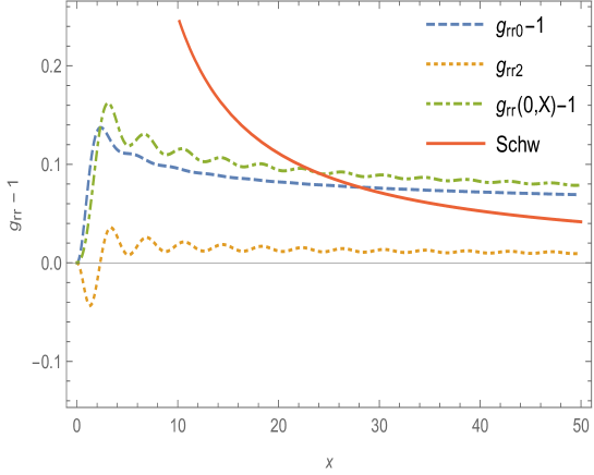
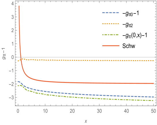
Figure 1: Metric coefficients $g_{rr}-1$ and $-g_{tt}-1$ and their respective two first terms, $g_{rr0}-1$, $g_{rr2}$ (top) and $-g_{tt0}-1$, $-g_{tt2}$ (bottom) for a central value $\sigma(x=0)=0.4,$ $\nu_{0}(x=0)=-0.11$, $\nu_{1}(x=0)=0.17,$ $\mu_{0}(x=0)=0.11,$ $\mu_{1}(x=0)=-0.17$ according to explained in the text and the Schwarzschild metric coefficients are also shown for the solution of the same mass.

In Figs. 2. and 3. the answers for differential equations mentioned by Eqs. (21-25) are shown.

As we can see from Fig. 3. the radial part of scalar field, $\sigma$, with a damping decrease becomes negative for some values of $x$ . This means that negative scalar fields have an effective role in being of oscillatons.

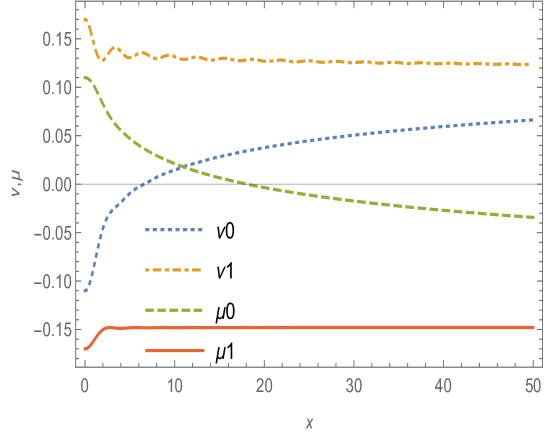
Figure 2: Metric functions $\nu_{0},$ $\nu_{1},$ $\mu_{0}$ and $\mu_{1}$with the initial boundary conditions mentioned in Fig. 1.

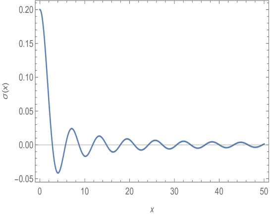
Figure 3: Radial part of the scalar field with the boundary conditions mentioned in Fig. 1 and 2.

Similar to what has been done for metric coefficient, we can rewrite the energy density, Eq. (3), the radial pressure, Eq. (5) and the angular pressure, Eq. (6) for oscillaton as

$\rho_{\Phi}(t,x)=\frac{1}{8\pi}m_{pl}^{2}m_{\Phi}^{2}\{\sigma^{2}e^{-(\nu-\mu)}[1-cos(2\omega t)]+\sigma^{\prime 2}e^{-(\nu+\mu)}[1+cos(2\omega t)]+\frac{\sigma^{4}}{2}[cos(4\omega t)+4cos(2\omega t)+3]\}$                                                            (28)

$p_{r}(t,x)=\frac{1}{8\pi}m_{pl}^{2}m_{\Phi}^{2}\{\sigma^{2}e^{-(\nu-\mu)}[1-cos(2\omega t)]+\sigma^{\prime 2}e^{-(\nu+\mu)}[1+cos(2\omega t)]-\frac{\sigma^{4}}{2}[cos(4\omega t)+4cos(2\omega t)+3]\}$                                                            (29)

$p_{\bot}(t,x)=\frac{1}{8\pi}m_{pl}^{2}m_{\Phi}^{2}\{\sigma^{2}e^{-(\nu-\mu)}[1-cos(2\omega t)]-\sigma^{\prime 2}e^{-(\nu+\mu)}[1+cos(2\omega t)]-\frac{\sigma^{4}}{2}[cos(4\omega t)+4cos(2\omega t)+3]\}$                                                            (30)

Equations 28-30 show that different nodes of energy density, radial and angular components of pressure can be obtained easily through their expansion. The values of $\rho_{\Phi}$ for times $\omega t=0$, $\frac{\pi}{2}$ and $\rho_{\Phi 0}$ using the Fourier expansion to second order are shown in Fig. 4.

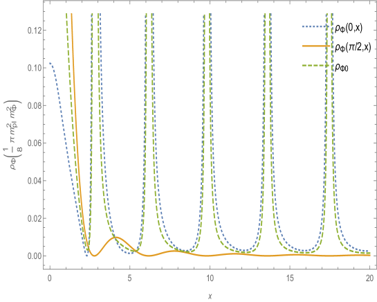
Figure 4: The energy density function $\rho_{\Phi}(\omega t,x)$ (see Eq. 28) for the oscillaton in Fig. 1, 2.

The values calculated for the components of radial and angular pressure for times $\omega t=0,\frac{\pi}{2}$ and zero nodes are shown in Fig. 5. As we can see from Fig. 5. both radial and angular components have a negative effective pressure for some values of $x$. This means that for negative pressure work is done on the oscillaton when it expands. On the other hand by using Eq . (4) and (16) we can also evaluate the momentum density of the oscillaton. The values of $p_{\Phi}$ for times $\omega t=0,\frac{\pi}{2}$ are shown in Fig. 5. As we can see from Figs.4 and 5.

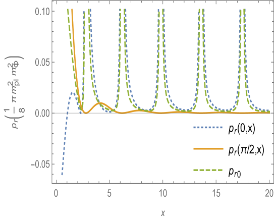
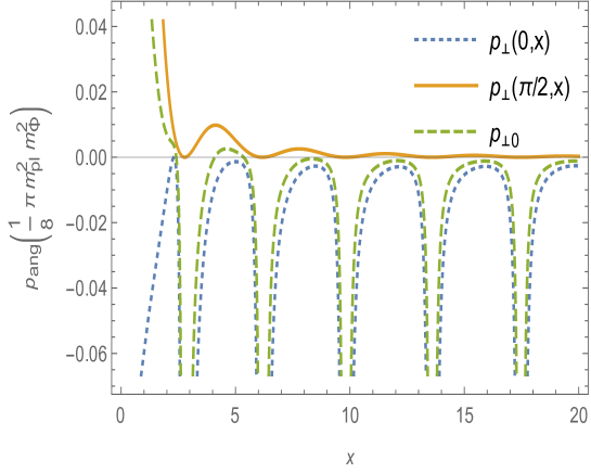
Figure 5: The radial pressure function $p_{r}(\omega t,x)$ (see Eq. 29) (top) and angular pressure function $p_{\bot}(\omega t,x)$ (see Eq. 30 ) (bottom) for the solutions in Fig. 1, 2.

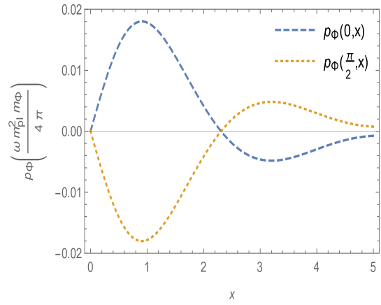
Figure 6: The momentum density function for the solutions in Fig. 1, 2.

Since the metric coefficients are asymptotically flat, static and comply with their corresponding ones in the Minkowski situation when $x\rightarrow\infty$, therefore $exp(\nu+\mu)$ is identified as $\frac{1}{1-\frac{2GM_{\Phi}}{r}}$ . Then the mass seen by an observer at infinity may be calculated as [7-9]

This is the mass which is related to the scalar field and can be employed as a possibility for the role of dark matter. Equation (31) shows that the calculated mass of the oscillaton is constant which means that the masses observed at infinity are the same for all times. This is natural because oscillaton should be in line with the Schwarzschild solution for the same mass according to Birkhoff^,s theorem[13]. Here some thing is unusual, and that is, for $\sigma(x=0)<0.235$ the mass obtained from the Eq. (31) is negative. We can see that there is a negative maximum mass $M_{max}=-0.23377m_{Pl}^{2}/m$ with $\sigma_{c}(x=0)=0.175.$ Whereas the $p_{r}(0,x)$ (main component of radial pressure) at least for these mentioned values, $\sigma(x=0)<0.235,$ are negative. The closest known real representative of such exotic matter is a region of pseudo-negative pressure density produced by the Casimir effect [14-17]. Therefore the negative mass can be described by this model, quartic potential, the advantage which distinguishes this model from quadratic and exponential scalar potential. For values higher than $\sigma(x=0)>0.235$ the mass values are positive and increase rapidly.

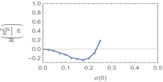
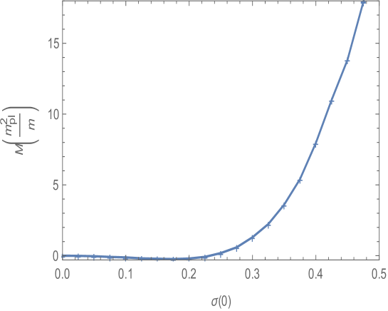
Figure 7: The mass observed at infinity (equation 31) for different central values of $\sigma(0)$.

As we mentioned in boundary conditions, the fundamental frequency is obtained by asymptotic value $exp(\nu-\mu)(\infty)=\Omega^{-2}$. In that we had $\mu_{0}(\infty)=-\nu_{0}(\infty)\neq 0$ due to the boundary conditions and taking into account the rapid convergence of $\nu_{0}$ (Fig. 2), then we can have

$\Omega=e^{-\nu_{0}(\infty)}$.                                      (32)

The profile of the fundamental frequencies are shown in Fig. 8. It is clear that more massive oscillatons oscillate with smaller frequencies.

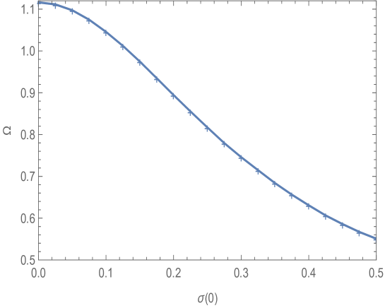
Figure 8: The fundamental frequencies $\Omega$ for corresponding masses shown in Fig. 7.

IV. THE STATIONARY LIMIT PROCEDURE

For weak field condition in which $\sigma(0)\ll 1$ (in consequence |$\mu_{1}|\ll 1$ ), It is easy to simplify the Eqs. (21-25) as far as possible as

$\nu_{0}^{\prime}=x[e^{2\mu_{0}}\sigma^{2}+\sigma^{\prime 2}]$,                                  (33)

$\mu_{0}^{\prime}=\frac{1}{x}\{1+e^{\nu_{0}+\mu_{0}}(\frac{3}{2}x^{2}\sigma^{4}-1)\},$                   (34)

$\mu_{1}^{\prime}=\sigma e^{\nu_{0}+\mu_{0}}(x^{2}-1)$,                                (35)

$\sigma^{\prime\prime}=-\sigma^{\prime}(\frac{2}{x}-\mu_{0}^{\prime})-3\sigma^{3}e^{\nu_{0}+\mu_{0}}-\sigma e^{2\mu_{0}},$           (36)

where for $z\ll 1$, we have used this fact that $I_{0}(z)\sim\mathcal{O}(1)$, $I_{1}(z)\sim\mathcal{O}(\frac{z}{2})$ and higher orders, $I_{n}(z)$ , are neglected, while Eq. (18-c) with regard to variable changes mentioned in Eq. (20) remains without change.

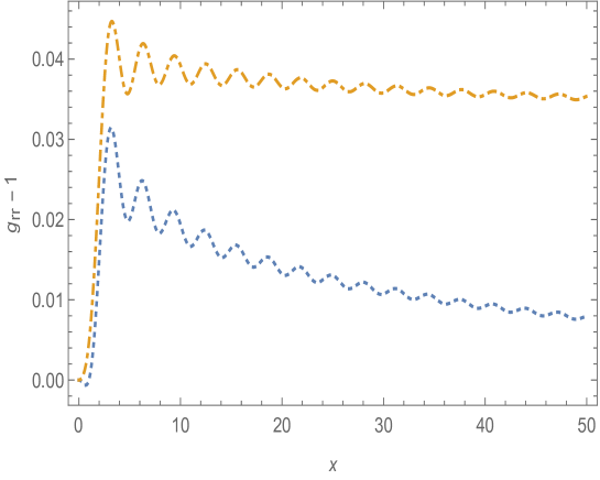
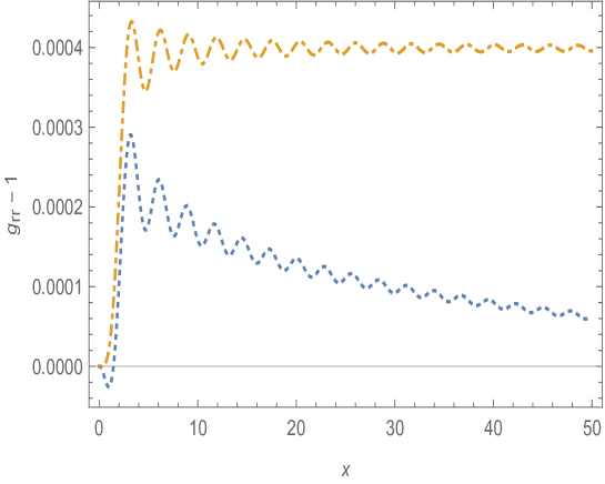
Figure 9: Comparison of the numerical results for the metric coefficient $g_{rr}-1$ for a quartic scalar potential oscillaton calculated by the method of sec.III (dotted) and with the stationary limit procedure (dotDashed) for two different central values of $\sigma(0)=0.2$ (top) and $\sigma(0)=0.02$ (bottom).

If we expand the scalar potential in a Fourier series by taking Eq. (16)

$V(\Phi)=\stackrel{{\scriptstyle[}}{{n}}=0]{4}{\sum}V_{n}(\sigma)cos(n\omega t)=\frac{m_{\varPhi}^{2}m_{Pl}^{2}}{16\pi}\sigma^{4}[cos(4\omega t)+4cos(2\omega t)+3]$,           (37)

then, as we have $\lambda=m_{\Phi}^{2}k_{0}$ , then we can obtain

$\sigma=(\frac{16\pi V_{0}(\sigma)}{m_{Pl}^{2}m_{\varPhi}^{2}})^{\frac{1}{4}}$.                                      (38)

It is clear that Eq. (36) is the only equation which will change among (33-36). Therefore it can be rewritten as

$\sigma^{\prime\prime}=-\sigma^{\prime}(\frac{2}{x}-\mu_{0}^{\prime})-3(\frac{16\pi V_{0}(\sigma)}{m_{Pl}^{2}m_{\varPhi}^{2}})^{\frac{1}{4}}e^{\nu_{0}+\mu_{0}}-(\frac{16\pi V_{0}(\sigma)}{m_{Pl}^{2}m_{\varPhi}^{2}})e^{2\mu_{0}}.$         (39)

At this stage it is necessary to recall that, since oscillatons are made of real scalar fields, therefore we know from non-relativistic field theory that charge and current densities which are identified as $\rho$ and $\overrightarrow{J}$ respectively should be equal to zero, then these objects are electrically neutral. On the other hand real $\Phi$ corresponds to electrically neutral particles in the oscillaton environment, hence we do not expect any electromagnetic wave emitting from oscillatons [9].

Another interesting thing is that: Could the oscillatons predicted by the scalar field be somehow associated with the ”gravitational waves” phenomenon?

As a motivation for the this issue, we start with the following reasoning. In the actual status of our understanding of the universe, there is an apparent asymmetry in the kind of interactions that take part in nature. The Scalar Field Dark Matter Model: A Braneworld Connection known fundamental interactions are either spin-1, or spin-2. Electromagnetic, weak and strong interactions are spin-1 interactions, while gravitational interactions are spin-2. Of course, this could be just a coincidence. Nevertheless, we know that the simplest particles are the spin-0 ones. The asymmetry lies in the fact that there is no spin-0 fundamental interactions. Why did Nature forget to use spin-0 fundamental interactions? On the other hand, we know from the success of the $\Lambda CDM$ model that two fields currently take the main role in the Cosmos, the dark matter and the dark energy. Recently, it has been indeed proposed that dark matter is a scalar field, that is, a spin-0 fundamental interaction. This is the so called Scalar Field Dark Matter $(SFDM)$ hypothesis . If true, this hypothesis could solve the problem of the apparent asymmetry in our picture of nature [18]. As a final part of this work, it is interesting to do a comparison between these kinds of oscillatons made by quartic scalar potential and our previous work which described by exponential scalar potential [9]. For quartic scalar potential, metric coefficients, for different values of $\sigma$ , comply with flatness condition asymptotically much more better than their corresponding ones in exponential scalar potential as well as frequencies. But in contrast to exponential and quadratic scalar potential we have several singularity points in energy density, radial and angular components of pressure in this kind of potential with no persuasive explanation [7, 9].

IV. CONCLUSIONS

In this paper we presented the simplest approximation for solving the minimally coupled Einstein-Klein-Gordon equations for a spherically symmetric oscillating soliton object endowed with a scalar quartic potential field $V(\Phi)=\frac{1}{4}\lambda\varPhi^{4}$ and an harmonic time-dependent scalar field $\Phi.$ By taking into account the Fourier expansions of differential equations and with regard to the boundary conditions which require the non-singularity and asymptotically flatness, solutions are obtained easily. It should be emphasized that a dynamical situation is imposed on the region of the oscillaton only, therefore we have asymptotically static metric and solutions. This fact helps us to find the mass of these astronomical objects as the most important topics to justify what called dark matter as well as their fundamental frequency. Results show that a quartic scalar field potential causes different profiles for metric functions and metric coefficients as well as energy density and mass distribution in comparison with what has been done in previous works for quadratic and exponential scalar field potentials. On the other hand with the same boundary initial conditions, all kind of the potentials, have the same fundamental frequency and mass relations [6,7,9]. Nevertheless, there are some more problems that should be investigated for oscillatons derived from a quartic scalar field. Here are some of these problems:

• In Fourier expansion, we have used to second order only for simplicity and higher order requires more complex calculation.

• For quartic potential studied in this research for $\sigma(x=0)<0.235$ we have negative mass which can be justified by Casimir effect and negative pressure, but more research should be carried out in this field.

• For $\sigma(x=0)>0.325,$ the mass values increase rapidly.

References

- [1] Jonathan L. Feng, arXiv: 1003.0904v2 [astro-ph], 2010.
- [2] Alexandre Arbey, Julien Lesgourguesc and Pierre Salatia, arXiv: astro-ph/0112324v2, 2002.
- [3] W. Buchmüller, C. Lüdeling, arXiv: hep-ph/0609174v1, 2006.
- [4] Tanja Rindler-Daller and Paul R. Shapiro,arXiv: 1312.1734v2 [astro-ph.Co] 2014.
- [5] T. Matos and F. S. Guzmán, Class. Quantum Grav. 18, 5055 (2001).
- [6] T. Matos, F. S. Guzmán , L. A Ureña- López and D. Núñez, arXiv: astro- ph/ 0102419.
- [7] L. Arturo Uréna-López, arXiv: gr-qc/0104093v3, 2002.
- [8] L. Arturo Ureña- López, Tonatiuth Matos and Ricardo Becerril qu-gr. 19 (2002) 6259-6277.
- [9] B. Malakolkalami, A. Mahmoodzadeh, Phys. Rev. D 94.103505 (2016).
- [10] Tonatiuh Matos and F. Siddhartha Guzmán, arXiv: gr-qc/0108027v1, 2001.
- [11] R. Friedberg, T. D. Lee and Y. Pang, Phys. Rev. D 35, 3640 (1987).
- [12] E. Seidel and W.-M. Suen, Phys. Rev. Lett. 66.1659 (1991).
- [13] S. Weinberg, Gravitation and Cosmology (John Wiley and Sons, Inc., New York, 1972), p. 337.
- [14] Astrid Lambrecht and The Casimir effect: a force from nothing, IOP publishing Ltd 2008, ISSN:0953-8585.
- [15] Astrid Lambrecht and Serge Reynuaud, Casimir effect and experiments, arxiv:1112.1301v1 [quantum-ph] 2011.
- [16] Saossen Mbarek and M. B. Paranjape, Negative mass bubbles in de Sitter space-time, arXive: 1407.145v2 [gr-qc] 2014.
- [17] J. P. Petit, Negative Mass Hypothesis In Cosmology And The Nature Of Dark Energy, Astrophysics and Space Science, 354, 2014.
- [18] Tonatiuh Matos, Luis Arturo Ureña- López, Miguel Alcubierre, Ricardo Becerril, Francisco S. Guzmán, and Darío Núñez, The Scalar Field Dark Matter Model: A Braneworld Connection, Lect. Notes Phys. 646, 401–420 (2004).