Angular momentum evolution of galaxies over the past 10 Gyr: A MUSE and KMOS dynamical survey of 400 star-forming galaxies from $z$ = 0.3–1.7

Abstract

We present a MUSE and KMOS dynamical study 405 star-forming galaxies at redshift $z$ = 0.28–1.65 (median redshift $\bar{z}$ = 0.84). Our sample are representative of star-forming, main-sequence galaxies, with star-formation rates of SFR = 0.1–30 M_⊙ yr^-1 and stellar masses M_⋆ = 10⁸–10¹¹ M_⊙. For 49 $\pm$ 4% of our sample, the dynamics suggest rotational support, 24 $\pm$ 3% are unresolved systems and 5 $\pm$ 2% appear to be early-stage major mergers with components on 8–30 kpc scales. The remaining 22 $\pm$ 5% appear to be dynamically complex, irregular (or face-on systems). For galaxies whose dynamics suggest rotational support, we derive inclination corrected rotational velocities and show these systems lie on a similar scaling between stellar mass and specific angular momentum as local spirals with $j_{\star}$ = $J$ / $M_{\star}\propto M_{\star}^{2/3}$ but with a redshift evolution that scales as $j_{\star}\,\propto$ M${}_{\star}^{2/3}(1+z)^{-1}$. We also identify a correlation between specific angular momentum and disk stability such that galaxies with the highest specific angular momentum (log($j_{\star}$ / M${}_{\star}^{2/3}$) $>$ 2.5) are the most stable, with Toomre $Q$ = 1.10 $\pm$ 0.18, compared to $Q$ = 0.53 $\pm$ 0.22 for galaxies with log($j_{\star}$ / M${}_{\star}^{2/3}$) $<$ 2.5. At a fixed mass, the HST morphologies of galaxies with the highest specific angular momentum resemble spiral galaxies, whilst those with low specific angular momentum are morphologically complex and dominated by several bright star-forming regions. This suggests that angular momentum plays a major role in defining the stability of gas disks: at $z\sim$ 1, massive galaxies that have disks with low specific angular momentum, are globally unstable, clumpy and turbulent systems. In contrast, galaxies with high specific angular have evolved in to stable disks with spiral structure where star formation is a local (rather than global) process.

1 Introduction

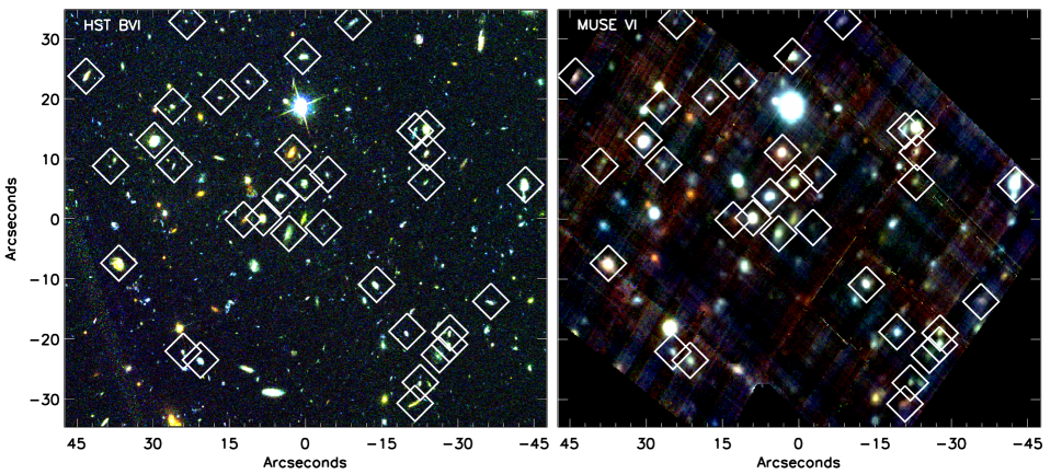
Figure 1: $HST$ and MUSE images for one of our survey fields, TN J1338$-$13 which contains a $z$ = 4.4 radio galaxy – underlining the fact that our survey of the foreground galaxy population is unbiased. Left: $HST$ $BVI$-band colour image. The [Oii] emitters identified from this field are also marked by open symbols. Center: MUSE $VI$-band colour image of the cube generated from three equal wavelength ranges. The [Oii] emitters are again marked. Each image is centered with (0,0) at $\alpha$: 13 38 26.1, $\delta$: $-$19 42 30.5 with North up and East left.

Identifying the dominant physical processes that were responsible for the formation of the Hubble sequence has been one of the major goals of galaxy formation for decades (Roberts, 1963; Gallagher & Hunter, 1984; Sandage, 1986). Morphological surveys of high-redshift galaxies, in particular utilizing the high angular resolution of the Hubble Space Telescope; (HST) have suggested that only at $z\sim$ 1.5 did the Hubble sequence begin to emerge (e.g.  Bell et al., 2004; Conselice et al., 2011), with the spirals and ellipticals becoming as common as peculiar galaxies (e.g.  Buitrago et al., 2013; Mortlock et al., 2013). However, galaxy morphologies reflect the complex (non-linear) processes of gas accretion, baryonic dissipation, star formation and morphological transformation that have occured during the history of the galaxy. Furthermore, morphological studies of high-redshift galaxies are subject to K-corrections and structured dust obscuration, which complicates their interpretation.

The more fundamental physical properties of galaxies are their mass, energy and angular momentum, since these are related to the amount of material in a galaxy, the linear size and the rotational velocity. As originally suggested by Sandage et al. (1970), the Hubble sequence of galaxy morphologies appears to follow a sequence of increasing angular momentum at a fixed mass (e.g.  Fall, 1983; Fall & Romanowsky, 2013; Obreschkow & Glazebrook, 2014). One route to identifying the processes responsible for the formation of disks is therefore to measure the evolution of the mass, size and dynamics (and hence angular momentum) of galaxy disks with cosmic time – properties which are more closely related to the underlying dark matter halo.

In the cold dark matter paradigm, baryonic disks form at the centers of dark matter halos. As dark matter halos grow early in their formation history, they acquire angular momentum ($J$) as a result of large scale tidal torques. The angular momentum acquired has strong mass dependence, with $J\propto M_{\rm halo}^{5/3}$ (e.g.  Catelan & Theuns, 1996). Although the halos acquire angular momentum, the centrifugal support of the baryons and dark matter within the virial radius is small. Indeed, whether calculated through linear theory or via $N$-body simulations, the “spin” (which defines the ratio of the halo angular speed to that required for the halo to be entirely centrifugally supported) follows approximately a log-normal distribution with average value $\lambda_{\rm DM}$ = 0.035 (Bett et al., 2007). This quantity is invariant to cosmological parameters, time, mass or environment (e.g.  Barnes & Efstathiou, 1987; Steinmetz & Bartelmann, 1995; Cole & Lacey, 1996).

As the gas collapses within the halo, the baryons can both lose and gain angular momentum between the virial radius and disk scale. If the baryons are dynamically cold, they fall inwards, weakly conserving specific angular momentum. Although the spin of the baryon at the virial radius is small, by the time they reach $\sim$ 2–10 kpc (the “size” of a disk), they form a centrifugally supported disk which follows an exponential mass profile (e.g.  Fall, 1983; Mo et al., 1998). Here, “weakly conserved” is within a factor of two, and indeed, observational studies suggest that late-type spiral disks have a spin of $\lambda_{\rm disk}^{\prime}$ = 0.025; (e.g.  Courteau, 1997), suggesting that that that only $\sim$ 30% of the initial baryonic angular momentum is lost due to viscous angular momentum redistribution and selective gas losses which occurs as the galaxy disks forms (e.g.  Burkert, 2009).

In contrast, if the baryons do not make it in to the disk, are redistributed (e.g. due to mergers), or blown out of the galaxy due to winds, then the spin of the disk is much lower than that of the halo. Indeed, the fraction of the initial halo angular momentum that is lost must be as high as $\sim$ 90% for early-type and elliptical galaxies (at the same stellar mass as spirals; Bertola & Capaccioli 1975), with Sa and S0 galaxies in between the extremes of late-type spiral- and elliptical- galaxies (e.g.  Romanowsky & Fall, 2012).

Numerical models have suggested that most of the angular momentum transfer occurs at epochs ealier than $z\sim 1$, after which the baryonic disks gain sufficient angular momentum to stabilise themselves (Dekel et al., 2009; Ceverino et al., 2010; Obreschkow et al., 2015; Lagos et al., 2016). For example, Danovich et al. (2015) use identify four dominant phases of angular momentum exchange that dominate this process: linear tidal torques on the gas beyond and through the virial radius; angular momentum transport through the halo; and dissipation and disk instabilities, outflows in the disk itself. These processes can increase and decrease the specific angular momentum of the disk as it forms, although they eventually “conspire” to produce disks that have a similar spin distribution as the parent dark matter halo.

Measuring the processes that control the internal redistribution of angular momentum in high-redshift disks is observationally demanding. However, on galaxy scales (i.e. $\sim$ 2–10 kpc), observations suggest redshift evolution according to $j_{\star}$ = J_⋆ / M${}_{\star}\propto$(1+$z$)ⁿ with $n\sim$ $-$1.5, at least out to $z\sim$ 2 (e.g.  Obreschkow et al., 2015; Burkert et al., 2015). Recently, Burkert et al. (2015) exploited the kmos^3D survey of $z\sim$ 1–2.5 star-forming galaxies at to infer the angular momentum distribution of baryonic disks, finding that their spin is is broadly consistent the dark matter halos, with $\lambda\sim$ 0.037 with a dispersion ($\sigma_{\rm log\lambda}\sim$ 0.2). The lack of correlation between the “spin” ($j_{\rm disk}$ / $j_{\rm DM}$) and the stellar densities of high-redshift galaxies also suggests that the redistribution of the angular momentum within the disks is the dominant process that leads to compactation (i.e. bulge formation; Burkert et al. 2016; Tadaki et al. 2016). Taken together, these results suggest that angular momentum in high redshift disks plays a dominant role in “crystalising” the Hubble sequence of galaxy morphologies.

In this paper, we investigate how the angular momentum and spin of baryonic disks evolves with redshift by measuring the dynamics of a large, representative sample of star-forming galaxies between $z\sim$ 0.28–1.65 as observed with the KMOS and MUSE integral field spectrographs. We aim to measure the angular momentum of the stars and gas in large and representative samples of high-redshift galaxies. Only now, with the capabilities of sensitive, multi-deployable (or wide-area) integral field spectrographs, such as MUSE and KMOS, is this becoming possible (e.g.  Bacon et al., 2015; Wisnioski et al., 2015; Stott et al., 2016; Burkert et al., 2015). We use our data to investigate how the mass, size, rotational velocity of galaxy disks evolves with cosmic time. As well as providing constraints on the processes which shape the Hubble sequence, the evolution of the angular momentum and stellar mass provides a novel approach to test galaxy formation models since these values reflect the initial conditions of their host halos, merging, and the prescriptions that describe the processes of gas accretion, star formation and feedback, all of which can strongly effect the angular momentum of the baryonic disk.

In §2 we describe the observations and data reduction. In §3 we describe the analysis used to derive stellar masses, galaxy sizes, inclinations, and dynamical properties. In §4 we combine the stellar masses, sizes and dynamics to measure the redshift evolution of the angular momentum of galaxies. We also compare our results to hydro-dynamical simulations. In §5 we give our conclusions. Throughout the paper, we use a cosmology with $\Omega_{\Lambda}$ = 0.73, $\Omega_{m}$ = 0.27, and H₀ = 72 km s^-1 Mpc^-1. In this cosmology a spatial resolution of 0.7^′′ corresponds to a physical scale of 5.2 kpc at $z$ = 0.84 (the median redshift of our survey). All quoted magnitudes are on the AB system and we adopt a Chabrier IMF throughout.

2 Observations and Data Reduction

The observations for this program were acquired from a series of programs (commissioning, guaranteed time and open-time projects; see Table 1) with the new Multi-Unit Spectroscopic Explorer (MUSE; Bacon et al. 2010, 2015) and $K$-band Multi-Object Spectrograph (KMOS; Sharples et al. 2004) on the ESO Very Large Telescope (VLT). Here, we describe the observations and data reduction, and discuss how the properties (star-formation rates and stellar masses) of the galaxies in our sample compare to the “main-sequence” population.

2.1 MUSE Observations

As part of the commissioning and science verification of the MUSE spectrograph, observations of fifteen “extra-galactic” fields were taken between 2014 February and 2015 February. The science targets of these programs include “blank” field studies (e.g. observations of the Hubble Ultra-Deep Field; Bacon et al. 2015), as well as high-redshift ($z>$ 2) galaxies, quasars and galaxy clusters (e.g. Fig. 1) (see also Husband et al., 2015; Richard et al., 2015; Contini et al., 2015). The wavelength coverage of MUSE (4770–9300 Å  in its standard configuration) allows us to serendipitously identify [Oii] emitters between $z\sim$ 0.3–1.5 in these fields and so to study the dynamics of star-forming galaxies over this redshift range. We exploit these observation to construct a sample of star-forming galaxies, selected via their [Oii] emission. The program IDs, pointing centers, exposure times, seeing FWHM (as measured from stars in the continuum images) for all of the MUSE pointings are given in Table 1. We also supplement these data with [Oii] emitters from MUSE observations from two open-time projects (both of whose primary science goals are also to detect and resolve the properties of $z>$ 3 galaxies/QSOs; Table 1). The median exposure time for each of these fields is 12 ks, but ranges from 5.4–107.5 ks. In total, the MUSE survey area exploited here is $\sim$ 20 arcmin² with a total integration time of 89 hours.

The MUSE IFU provides full spectral coverage spanning 4770–9300 Å  and a contiguous field of view of 60 ${}^{\prime\prime}\times$ 60 ^′′, with a spatial sampling of 0.2^′′ / pixel and a spectral resolution of $R$ = $\lambda$ / $\Delta\lambda$ = 3500 at $\lambda$ = 7000Å  (the wavelength of the [Oii] at the median redshift of our sample) – sufficient to resolve the [Oii]$\lambda\lambda$3726.2,3728.9 emission line doublet. In all cases, each 1 hour observing block was split in to a number of sub-exposures (typically 600, 1200, or 1800 seconds) with small (2^′′) dithers between exposures to account for bad pixels. All observations were carried out in dark time, good sky transparency. The average $V$-band seeing for the observations was 0.7^′′ (Table 1).

To reduce the data, we use the MUSE esorex pipeline which extracts, wavelength calibrates, flat-fields the spectra and forms each datacube. In all of the data taken after August 2014, each 1 hr science observation was interspersed with a flat-field to improve the slice-by-slice flat field (illumination) effects. Sky subtraction was performed on each sub-exposure by identifying and subtracting the sky emission using blank areas of sky at each wavelength slice, and the final mosaics were then constructed using an average with a 3-$\sigma$ clip to reject cosmic rays, using point sources in each (wavelength collapsed) image to register the cubes. Flux calibration was carried out using observations of known standard stars at similar airmass and were taken immediately before or after the science observations. In each case we confirmed the flux calibration by measuring the flux density of stars with known photometry in the MUSE science field.

Table 1: Observing logs

Field Name	PID	RA	Dec	$t_{\rm exp}$	seeing	3-$\sigma$ SB limit
		(J2000)	(J2000)	($ks$)	(′′)
MUSE:
J0210-0555	060.A-9302	02:10:39.43	$-$05:56:41.28	9.9	1.08	9.1
J0224-0002	094.A-0141	02:24:35.10	$-$00:02:16.00	14.4	0.70	11.0
J0958+1202	094.A-0280	09:58:52.34	+12:02:45.00	11.2	0.80	15.2
COSMOS-M1	060.A-9100	10:00:44.26	+02:07:56.91	17.0	0.90	5.3
COSMOS-M2	060.A-9100	10:01:10.57	+02:04:10.60	12.6	1.0	6.3
TNJ1338	060.A-9318	13:38:25.28	$-$19:42:34.56	32.0	0.75	4.1
J1616+0459	060.A-9323	16:16:36.96	+04:59:34.30	7.0	0.90	7.6
J2031-4037	060.A-9100	20:31:54.52	$-$40:37:21.62	37.7	0.83	5.2
J2033-4723	060.A-9306	20:33:42.23	$-$47:23:43.69	7.9	0.85	7.4
J2102-3535	060.A-9331	21:02:44.97	$-$35:53:09.31	11.9	1.00	6.2
J2132-3353	060.A-9334	21:32:38.97	$-$33:53:01.72	6.5	0.70	13.6
J2139-0824	060.A-9325	21:39:11.86	$-$38:24:26.14	7.4	0.80	5.7
J2217+1417	060.A-9326	22:17:20.89	+14:17:57.01	8.1	0.80	4.9
J2217+0012	095.A-0570	22:17:25.01	+00:12:36.50	12.0	0.69	6.0
HDFS-M2	060.A-9338	22:32:52.71	$-$60:32:07.30	11.2	0.90	7.3
HDFS-M1	060.A-9100	22:32:55.54	$-$60:33:48.64	107.5	0.80	2.8
J2329-0301	060.A-9321	23:29:08.27	$-$03:01:58.80	5.7	0.80	5.6
KMOS:
COSMOS-K1	095.A-0748	09:59:33.54	+02:18:00.43	16.2	0.70	22.5
SSA22	060.A-9460	22:19:30.45	+00:38:53.34	7.2	0.72	31.2
SSA22	060.A-9460	22:19:41.15	+00:23:16.65	7.2	0.70	33.7

Notes: RA and Dec denote the field centers. The seeing is measured from stars in the field of view (MUSE) or from a star placed on one of the IFUs (KMOS). The units of the surface brightness limit are $\times$10^-19 erg s^-1 cm^-2 arcsec^-2. The reduced MUSE datacubes for these fields available at: http://astro.dur.ac.uk/$\sim$ams/MUSEcubes/

To identify [Oii] emitters in the cubes, we construct and coadd $V$- and $I$-band continuum images from each cube by collapsing the cubes over the wavelength ranges $\lambda$ = 4770–7050Å  and $\lambda$ = 7050–9300Å respectively. We then use sextractor (Bertin & Arnouts, 1996) to identify all of the $>$4 $\sigma$ continuum sources in the “detection” images. For each continuum source, we extract a 5 $\times$ 5^′′ sub-cube (centered on each continuum source) and search both the one and two-dimensional spectra for emission lines. At this resolution, the [Oii] doublet is resolved and so trivially differentiated from other emission lines, such as Ly$\alpha$, [Oiii] 4959,5007 or H$\alpha$+[Nii] 6548,6583. In cases where an emission line is identified, we measure the wavelength, $x$ / $y$ (pixel) position and RA / Dec of the galaxy. Since we are interested in resolved dynamics, we only include galaxies where the [Oii] emission line is detected above 5 $\sigma$ in the one dimensional spectrum. To ensure we do not miss any [Oii] emitters that do not have continuum counterparts, we also remove all of the continuum sources from each cube by masking a 5^′′ diameter region centered on the continuum counterpart, and search the remaining cube for [Oii] emitters. We do not find any additional [Oii]-emitting galaxies where the integrated [Oii] flux is detected above a signal-to-noise of 5 (i.e. all of the bright [Oii] emitters in our sample have at least a 4 $\sigma$ detection in continuum).

In Fig. 1 we show a HST $BVI$-band colour image of one of our target fields, TNJ 1338, along with a colour image generated from the 32 ks MUSE exposure. The blue, green and red channels are generated from equal width wavelength ranges between 4770–9300 AA  in the MUSE cube. In both panels we identify all of the [Oii] emitters. In this single field alone, there are 33 resolved [Oii] emitters.

From all 17 MUSE fields considered in this analysis, we identify a total of 431 [Oii] emitters with emission line fluxes ranging from 0.1–170 $\times$ 10^-17 erg s^-1 cm^-2 with a median flux of 3 $\times$ 10^-17 erg s^-1 cm^-2 and a median redshift of $z$ = 0.84 (Fig. 2).

Before discussing the resolved properties of these galaxies, we first test how our [Oii]-selected sample compares to other [Oii] surveys at similar redshifts. We calculate the [Oii] luminosity of each galaxy and in Fig. 2 show the [Oii] luminosity function in two redshift bins ($z$ = 0.3–0.8 and $z$ = 0.8–1.4). In both redshift bins, we account for the incompleteness caused by the exposure time differences between fields. We highlight the luminosity limits for four of the fields which span the whole range of depths in our survey. This figure shows that the [Oii] luminosity function evolves strongly with redshift, with $L^{\star}$ evolving from log₁₀($L^{\star}$[erg s^-1 cm^-2]) = 41.06 $\pm$ 0.17 at $z$ = 0 to log₁₀($L^{\star}$[erg s^-1 cm^-2]) = 41.5 $\pm$ 0.20 and log₁₀($L^{\star}$[erg s^-1 cm^-2]) = 41.7 $\pm$ 0.22 at $z$ = 1.4 (see also Ly et al., 2007; Khostovan et al., 2015). The same evolution has also been seen in at UV wavelengths (Oesch et al., 2010) and in H$\alpha$ emission (e.g.  Sobral et al., 2013a).

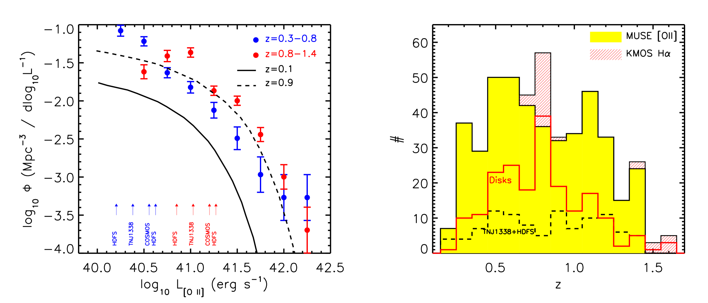
Figure 2: Left: [Oii] luminosity function for the star-forming galaxies in our sample from the 18 MUSE IFU pointings. We split the sample in two redshift bins, $z$ = 0.3–0.8 and $z$ = 0.8–1.4. The arrows on the plot denote luminosity limits for four of the fields in the MUSE sample (which span the complete range of depths). To baseline these results, we overlay the [Oii] luminosity function at $z$ = 0 from SDSS (Ciardullo et al., 2013) which shows that there is strong evolution in L${}^{\star}_{\rm[OII]}$ from $z\sim$ 0 to $z\sim$ 0.5. This evolution is also seen in other [Oii] surveys (e.g.  Ly et al., 2007; Khostovan et al., 2015). Right: The redshift distribution of the [Oii] and H$\alpha$ emitters in our MUSE and KMOS samples. Our sample has a median redshift of $z$ = 0.84 and a full redshift range of $z$ = 0.28–1.67. Since the MUSE observations have a wide range of exposure times, from 5.7–107.5 ks, we overlay the redshift distribution of the [Oii] emitters in the two deepest fields, HDFS and TNJ 1338, to highlight that the highest-redshift galaxies are not dominated by the deepest observations. We also overlay the redshift distribution of the galaxies classified as “rotationally supported” (i.e. disks).

2.2 KMOS Observations

We also include observations of the redshifted H$\alpha$ in 46 $z\sim$0.8–1.7 galaxies from three well-studied extra-galactic fields. Two of these fields are taken from an H$\alpha$-selected sample at $z$ = 0.84 from the KMOS–Hi-$z$ emission line survey (KMOS-HiZELS; Geach et al. 2008; Sobral et al. 2009, 2013a) and are discussed in Sobral et al. (2013b, 2015) and Stott et al. (2014). Briefly, observations of 29 H$\alpha$-selected galaxies were taken between 2013 June and 2013 July using KMOS with the $YJ$-band filter as part of the KMOS science verification programme. The near–infrared KMOS IFU comprises 24 IFUs, each of size 2.8 $\times$ 2.8^′′ sampled at 0.2^′′ which can be deployed across a 7-arcmin diameter patrol field. The total exposure time was 7.2 ks per pixel, and we used object-sky-object observing sequences, with one IFU from each of the three KMOS spectrographs placed on sky to monitor OH variations.

Further KMOS observations were also obtained between 2015 April 25 and April 27 as the first part of a 20-night KMOS guaranteed time programme aimed at resolving the dynamics of 300 mass-selected galaxies at $z\sim$ 1.2–1.7. Seventeen galaxies were selected from photometric catalogs of the COSMOS field. We initially selected targets in the redshift range $z$ = 1.3–1.7 and brighter than $K_{\rm AB}$ = 22 (a limit designed to ensure we obtain sufficient signal-to-noise per resolution element to spatially resolve the galaxies; see Stott et al. 2016 for details). To ensure that the H$\alpha$ emission is bright enough to detect and spatially resolve with KMOS, we pre-screened the targets using the Magellan Multi-object Infra-Red Spectrograph (mmirs) to search for and measure the H$\alpha$ flux of each target, and then carried out follow-up observations with KMOS of those galaxies with H$\alpha$ fluxes brighter than 5 $\times$ 10^-17 erg s^-1 cm^-2. These KMOS observations were carried out using the $H$-band filter, which has a spectral resolution of $R$ = $\lambda$ / $\Delta\lambda$ = 4000. We used object-sky-object sequences, with one of the IFUs placed on a star to monitor the PSF and one IFU on blank sky to measure OH variations. The total exposure time was 16.2 ks (split in to three 5.4 ks OBs, with 600 s sub-exposures). Data reduction was performed using the spark pipeline with additional sky-subtraction and mosaicing carried out using customized routines. We note that a similar dymamical / angular momemtum analysis of the $\sim$ 800 galaxies at $z\sim$ 1 from the KROSS survey are presented in Harrison et al. (2017).

2.3 Final Sample

Combining the two KMOS samples, in total there are 41 / 46 H$\alpha$-emitting galaxies suitable for this analysis (i.e. H$\alpha$ detected above a S / N $>$ 5 in the collapsed, one-dimensional spectrum). From our MUSE sample of 431 galaxies, 67 of the faintest [Oii] emitters are only detected above a S / N = 5 when integrating a 1 $\times$ 1^′′ region, and so no longer considered in the following analysis, leaving us with a sample of 364 [Oii] emitters for which we can measure resolved dynamics. Together, the MUSE and KMOS sample used in the following analysis comprises 405 galaxies with a redshift range $z$ = 0.28–1.63. We show the redshift distribution for the full sample in Fig. 2.

3 Analysis

With the sample of 405 emission-line galaxies in our survey fields, the first step is to characterize the integrated properties of the galaxies. In the following, we investigate the spectral energy distributions, stellar masses and star formation rates, sizes, dynamics, and their connection with the galaxy morphology, and we put our findings in the context of our knowledge of the general galaxy population at these redshifts. We first discuss their stellar masses.

3.1 Spectral Energy Distributions and Stellar Masses

The majority of the MUSE and KMOS fields in our sample have excellent supporting optical / near- and mid-infrared imaging, and so to infer the stellar masses and star formation rates for the galaxies in our sample, we construct the spectral energy distributions for each galaxy. In most cases, we exploit archival HST, Subaru, Spitzer / IRAC, UKIRT / WFCAM and / or VLT / Hawk-I imaging. In the optical / near-infrared imaging, we measure 2^′′ aperture photometry, whilst in the IRAC 3.6 / 4.5-$\mu$m bands we use 5^′′ apertures (and apply appropriate aperture corrections based on the PSF in each case). We list all of the properties for each galaxy, and show their broad-band SEDs in Table A1. We use hyper-z (Bolzonella et al., 2000) to fit the photometry of each galaxy at the known redshift, allowing a range of star formation histories from late to early types and redennings of A_V = 0–3 in steps of $\Delta$A_V = 0.2 and a Calzetti dust reddening curve (Calzetti et al., 2000). In cases of non detections, we adopt a 3$\sigma$ upper limit.

We show the observed photometry and overlay the best-fit hyper-z SED for all of the galaxies in our sample in Fig. A1–A3. Using the best-fit parameters, we then estimate the stellar mass of each galaxy by integrating the best-fit star-formation history, accounting for mass loss according to the starburst99 mass loss rates (Leitherer et al., 1999). We note that we only calculate stellar masses for galaxies that have detections in $>$3 wavebands, although include the best SEDs for all sources in Fig. A1–A3. Using the stellar masses and rest-frame $H$-band magnitudes, we derive a median mass-to-light ratio for the full sample of M_⋆ / L_H = 0.20 $\pm$ 0.01. The best-fit reddening values and the stellar masses for each galaxy are also given in Table A1.

As a consistency check that our derived stellar masses are consistent with those derived from other SED fitting codes, we compare our results with Muzzin et al. (2013) who derive the stellar masses of galaxies in the COSMOS field using the easy photometric redshift code (Brammer et al., 2008) with stellar mass estimated using fast Kriek et al. (2009). For the 54 [Oii] emitting galaxies in the COSMOS field in our sample, the stellar masses we derive are a factor 1.19 $\pm$ 0.06 $\times$ higher than those derived using fast. Most of this difference can be attributed to degeneracies in the redshifts and best-fit star-formation histories. Indeed, if we limit the comparison to galaxies where the photometric and spectroscopic redshifts agree within $\Delta z<$ 0.2, and where the luminosity weighted ages also agrees to within a factor of 1.5, then then the ratio of the stellar masses from hyper-z / easy are 1.02 $\pm$ 0.04 $\times$.

To place the galaxies we have identified in the MUSE and KMOS data in context of the general population at their respective redshifts, next we calculate their star formation rates (and specific star formation rates). We first calculate the [Oii] or H$\alpha$ emission luminosity (L_[OII] and L_Hα respectively). To account for dust obscuration, we adopt the best-fit stellar redenning (A_V) from the stellar SED returned by from hyper-z and convert this to the attenuation at the wavelength of interest (A_[OII] or A_Hα) using a Calzetti reddennign law; Calzetti et al. 2000). Next, we assume that the the gas and stellar phases are related by A_gas = A_⋆ (1.9 $-$ 0.15 A_⋆); (Wuyts et al., 2013), and then calculate the total star-formation rates using SFR = $C$ $\times$ 10^-42 L_[OII] 10${}^{0.4A_{\rm gas}}$ with $C$ = 0.82 and $C$ = 4.6 for the [Oii] and H$\alpha$ emitters respectively. The star formation rates of the galaxies in our sample range from 0.1–300 M_⊙ yr^-1. In Fig. 3 we plot the specific star-formation rate (sSFR = SFR / M_⋆) versus stellar mass for the galaxies in our sample. This also shows that our sample display a wide range of stellar masses and star-formation rates, with median and quartile ranges of log₁₀(M_⋆ / M_⊙) = 9.4 $\pm$ 0.9 and SFR = 4.7${}_{-2.5}^{+2.2}$ M_⊙ yr^-1. As a guide, in this plot we also overlay a track of constant star formation rate with SFR = 1 M_⊙ yr^-1. To compare our galaxies to the high-redshift star-forming population, we also overlay the specific star formation rate for $\sim$ 2500 galaxies from the HiZELS survey which selects H$\alpha$ emitting galaxies in three narrow redshifts slices at $z$ = 0.40, 0.84 and 1.47 (Sobral et al., 2013a). For this comparison, we calculate the star formation rates for the HiZELS galaxies in an identical manner to that for our MUSE and KMOS sample. This figure shows that the median specific star formation rate of the galaxies in our MUSE and KMOS samples appear to be consistent with the so-called “main-sequence” of star-forming galaxies at their appropriate redshifts.

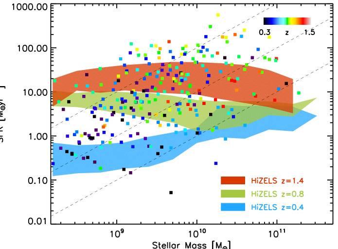
Figure 3: Star-formation rate versus mass for the galaxies in our sample (with points colour-coded by redshift). As a guide, we also overlay tracks of constant specific star formation rate (sSFR) with with sSFR = 0.1, 1 and 10 Gyr^-1. We also overlay the star formation rate–stellar mass relation at three redshift slices ($z$ = 0.40, 0.84 and 1.47) from the H$\alpha$ narrow-band selected sample from HiZELS (Sobral et al., 2013a). This shows that although the galaxies in our MUSE and KMOS samples span a wide range of stellar mass and star-formation rate, they are comparable to the general field population, with specific star formation rates sSFR $\sim$ 0.1–10 Gyr^-1.

3.2 Galaxy Sizes and Size Evolution

Next, we turn to the sizes for the galaxies in our sample. Studies of galaxy morphology and size, particularly from observations made with HST, have shown that the physical sizes of galaxies increase with cosmic time (e.g.  Giavalisco et al., 1996; Ferguson et al., 2004; Oesch et al., 2010). Indeed, late-type galaxies have continuum (stellar) half light radii that are on average a factor $\sim$ 1.5 $\times$ smaller at $z\sim$ 1 than at the present day (van der Wel et al., 2014; Morishita et al., 2014). As one of the primary aims of this study is to investigate the angular momentum of the galaxy disks, the continuum sizes are an important quantity.

We calculate the half light-radii in both continuum and emission lines for all galaxies in our sample. Approximately 60% of the galaxies in our sample have been observed with HST (using ACS / $BVI$ and / or WFC3 / $JH$-band imaging). Since we are interested in the extent of the stellar light, we measure the half light radius for each galaxy in the longest wavelength image available (usually ACS $I-$ or WFC $H$-band). To measure the half-light radius of each galaxy, we first fit a two-dimensional Sersic profile to the galaxy image to define an $x$ / $y$ center and ellipticity for the galaxy, and then measure the total flux within 1.5 $\times$ Petrosian radius and use the curve of growth (growing ellipses from zero to 1.5 $\times$ Petrosian aperture) to measure the half-light radius. A significant fraction of our sample do not have observations with HST and so we also construct continuum images from the IFU datacubes and measure the continuum size in the same way (deconvolving for the PSF). In Fig. 4 we compare the half-light radius of the galaxies in our sample from HST observations with that measured from the MUSE and KMOS continuum images. From this, we derive a median ratio of $r_{1/2,\rm HST}$ / $r_{1/2,\rm MUSE}$ = 0.97 $\pm$ 0.03 with a scatter of 30% (including unresolved sources in both cases).

For each galaxy in our sample, we also construct a continuum-subtracted narrow-band [Oii] or H$\alpha$ emission line image (using 200Å  on either size of the emission line to define the continuum) and use the same technique to measure the half-light radius of the nebular emission. The continuum and nebular emission line half light radii (and their errors) for each galaxy are given in Table A1. As Fig. 4 shows, the nebular emission is more extended that the continuum with $r_{1/2,\rm[OII]}$ / $r_{1/2,\rm HST}$ = 1.18 $\pm$ 0.03. This is consistent with recent results from the 3-D HST survey demonstrates that the nebular emission from $\sim$ $L^{\star}$ galaxies at $z\sim$ 1 tends to be systematically more extended than the stellar continuum (with weak dependence on mass; Nelson et al. 2015).

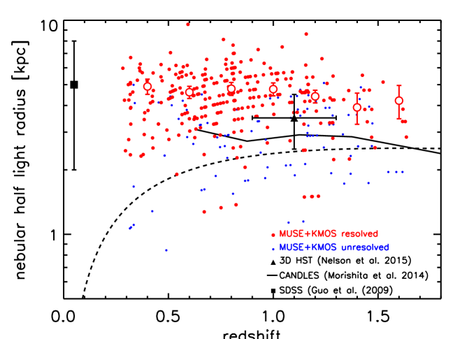
Figure 6: Evolution of the physical half-light radii with redshift for the galaxies in our sample. We plot the nebular emission line sizes in all cases ([O ii] for MUSE or H$\alpha$ for KMOS). We plot both the extended (red) and unresolved/compact (blue) galaxies individually, but also show the median half-light radii in $\Delta z$ = 0.2 bins as large filled points with errors (these medians include unresolved sources). We also include recent measurements of the nebular emission line half-light radii of $z\sim$ 1 galaxies from the 3D-HST survey (Nelson et al., 2015) and the evolution in the continuum sizes (corrected to nebular sizes using the results from Fig 4) from (Morishita et al., 2014) for galaxies in the CANDLES fields. We also include the size measurements from SDSS (Guo et al., 2009). As a guide, the dashed line shows the half light radius as a function of redshift for a 0.7^′′ PSF (the median seeing of our observations). This plot shows that the nebular emission half-light radii of the galaxies in our sample are consistent with similar recent measurements of galaxy sizes from HST (Nelson et al., 2015), and a factor $\sim$ 1.5 $\times$ smaller than late-type galaxies at $z$ = 0.

We also compare the continuum half light radius with the disk scale length, $R_{\rm d}$ (see § 3.4). From the data, we measure a $r_{\rm 1/2,HST}$ / $R_{\rm d}$ = 1.70 $\pm$ 0.05. For a galaxy with an exponential light profile, the half light radii and disk scale length are related by $r_{\rm 1/2}$ = 1.68 $R_{\rm d}$, which is consistent with our measurements (and we overlay this relation in Fig. 4). In Fig. 6 we plot the evolution of the half-light radii (in kpc) of the nebular emission with redshift for the galaxies in our sample which shows that the nebular emission half-light radii are consistent with similar recent measurements of galaxy sizes from HST (Nelson et al., 2015), and a factor $\sim$ 1.5 $\times$ smaller than late-type galaxies at $z$ = 0.

From the full sample of [Oii] or H$\alpha$ emitters, the spatial extent of the nebular emission of 75% of the sample are spatially resolved beyond the seeing, with little / no dependence on redshift, although the unresolved sources unsurprisingly tend to have lower stellar masses (median M${}_{\rm\star}^{\rm unresolved}$ = 1.0 $\pm$ 0.5 $\times$ 10⁹ M_⊙ compared to median M${}_{\rm\star}^{\rm resolved}$ = 3 $\pm$ 1 $\times$ 10⁹ M_⊙).

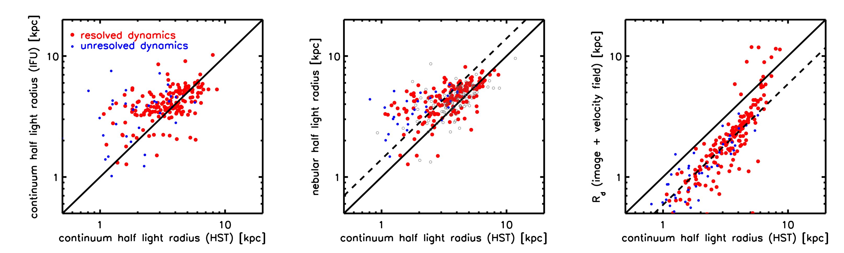
Figure 4: Comparison of the physical half-light radii of the galaxies in our sample as measured from HST and MUSE / KMOS imaging. Left: Continuum half-light radii as measured from HST broad-band imaging compared to those measured from the MUSE continuum image. Large red points denote sources that are resolved by MUSE or KMOS. Small blue point denote galaxies that are unresolved (or compact) in the MUSE or KMOS data. The median ratio of the half-light radii is $r_{\rm HST}$ / $r_{\rm MUSE}$ = 0.97 $\pm$ 0.03 (including unresolved sources and deconvolved for seeing). Center: Continuum half-light radius from HST versus nebular emission half-light radius (MUSE and KMOS) for the galaxies in our sample from MUSE and KMOS. The continuum and nebular emission line half-light radii are well correlated, although the nebular emission lines half-light radii are systematically larger than the continuum sizes, with $r_{\rm[OII]}$ / $r_{\rm HST}$ = 1.18 $\pm$ 0.03 (see also Nelson et al. 2015). Although not included in the fit, we also include on the plot the contuinuum size measurements from MUSE and KMOS as small grey points. These increase the scatter (as expected from the data in the left-hand panel), although the median ratio of nebular emission to continuum size is unaffected if these points are included. Right: Comparison of the disk scale length (measured from the dynamical modeling) versus the continuum half-light radius from HST. The median ratio of the half-light radius is larger than the disk radius by a factor $r_{\rm HST}$ / $R_{\rm d}$ = 1.70 $\pm$ 0.05, which is the consistent with that expected for an exponential disk.

3.3 Resolved Dynamics

Next, we derive the velocity fields and line-of-sight velocity dispersion maps for the galaxies in our sample. The two-dimensional dynamics are critical for our analysis since the circular velocity, which we will use to determine the angular momentum in § 4, must be taken from the rotation curve at a scale radius. The observed circular velocity of the galaxy also depends on the disk inclination, which can be determined using either the imaging, or dynamics, or both.

To create intensity, velocity and velocity dispersion maps for each galaxy in our MUSE sample, we first extract a 5 $\times$ 5^′′ “sub-cube” around each galaxy (this is increased to 7 $\times$ 7^′′ if the [Oii] is very extended) and then fit the [Oii] emission line doublet pixel-by-pixel. We first average over 0.6 $\times$ 0.6^′′ pixels and attempt the fit to the continuum plus emission lines. During the fitting procedure, we account for the increased noise around the sky OH residuals, and also account for the the spectral resolution (and spectral line spread function) when deriving the line width. We only accept the fit if the improvement over a continuum-only fit is $>$5 $\sigma$. If no fit is achieved, the region size is increased to 0.8 $\times$ 0.8^′′ and the fit re-attempted. In each case, the continuum level, redshift, line width, and intensity ratio of the 3726.2 / 3728.9Å  [Oii] emission line doublet is allowed to vary. In cases that meet the signal-to-noise threshold, errors are calculated by perturbing each parameter in turn, allowing the other parameters to find their new minimum, until a $\Delta\chi^{2}$ = 1-$\sigma$ is reached. For the KMOS observations we follow the same procedure, but fit the H$\alpha$ and [Nii] 6548,6583 emission lines. In Fig. 5 we show example images and velocity fields for the galaxies in our sample (the full sample, along with their spectra are shown in Appendix A). In Fig. 5 the first three panels show the HST image, with ellipses denoting the disk radius and lines identifying the major morphological and kinematic axis (see § 3.4), the MUSE $I$-band continuum image and the two-dimensional velocity field. We note that for each galaxy, the high-resolution image (usually from HST) is astrometrically aligned to the MUSE or KMOS cube by cross correlating the (line free) continuum image from the cube.

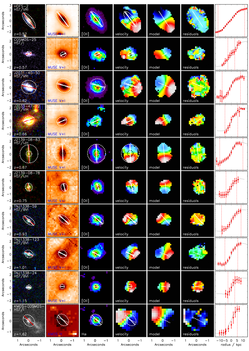
Figure 5: Example images and dynamics of nine galaxies in our sample. (a): HST colour image of each galaxy. given in each sub-image. The galaxies are ranked by increasing redshift. The ellipses denote the disk radius (inner ellipse R_d; outer ellipse 3 R_d). The cross denotes the dynamical center of the galaxy and the white-dashed and solid red line show the major morphological and kinematic axes respectively. (b): The continuum image from the IFU observations (dark scale denotes high intensity). The dashed lines are the same as in the first panel. (c): Nebular emission line velocity field. Dashed ellipses again show the disk radius at R_d and 3 R_d (the colour scale is set by the range shown in the final panel). (d): Best-fit two-dimensional dynamical model for each galaxy. In this panel, the cross and dashed line denote the dynamical center and major kinematic axis from our dynamical modeling. Residuals (data $-$ model) are shown in panel (e) on the same velocity scale as the velocity and best-fit model. The final panel shows the one-dimensional rotation curve, extracted along the major kinematic axis with a pseudo-slit of width 0.5 $\times$ FWHM of the seeing disk.

The ratio of circular velocity (or maximum velocity if the dynamics are not regular) to line-of-sight velocity dispersion ($V$ / $\sigma$) provides a crude, but common way to classify the dynamics of galaxies in to rotationally- version dispersion- dominated systems. To estimate the maximum circular velocity, $V$, we extract the velocity profile through the continuum center at a position angle that maximises the velocity gradient. We inclination correct this value using the continuum axis ratio from the broad-band continuum morphology (see § 3.4). For the full sample, we find a range of maximum velocity gradients from 10 to 540 km s^-1 (peak-to-peak) with a median of 98 $\pm$ 5 km s^-1 and a quartile range of 48–192 km s^-1. To estimate the intrinsic velocity dispersion, we first remove the effects of beam-smearing (an effect in which the observed velocity dispersion in a pixel has a contribution from the intrinsic dispersion and the flux-weighted velocity gradient across that pixel due to the PSF). To derive the intrinsic velocity dispersion, we calculate and subtract the luminosity weighted velocity gradient across each pixel and then calculate the average velocity dispersion from the corrected two-dimensional velocity dispersion map. In this calculation, we omit pixels that lie within the central PSF FWHM (typically $\sim$ 0.6^′′; since this is the region of the galaxy where the beam-smearing correction is most uncertain). For our sample, the average (corrected) line-of-sight velocity dispersion is $\sigma$ = 32 $\pm$ 4 km s^-1 (in comparison, the average velocity dispersion measured from the galaxy integrated one-dimensional spectrum is $\sigma$ = 70 $\pm$ 5 km s^-1). This average intrinsic velocity dispersion at the median redshift of our sample ($z$ = 0.84) is consistent with the average velocity dispersion seen in a number of other high-redshift samples (e.g.  Förster Schreiber et al., 2009; Law et al., 2009; Gnerucci et al., 2011; Epinat et al., 2012; Wisnioski et al., 2015).

For the full sample of galaxies in our survey, we derive a median inclination corrected ratio of $V$ / $\sigma$ = 2.2 $\pm$ 0.2 with a range of $V$ / $\sigma$ = 0.1–10 (where we use the limits on the circular velocities for galaxies classed as unresolved or irregular / face-on). We show the full distribution in Fig. 7.

Although the ratio of $V$ / $\sigma$ provides a means to separate “rotationally dominated” galaxies from those that are dispersion supported, interacting or merging can also be classed as rotationally supported. Based on the two-dimensional velocity field, morphology and velocity dispersion maps, we also provide a classification of each galaxy in four broad groups (although in the following dynamical plots, we highlight the galaxies by $V$ / $\sigma$ and their classification):

(i) Rotationally supported: for those galaxies whose dynamics appear regular (i.e. a spider-line pattern in the velocity field, the line-of-sight velocity dispersion peaks near the dynamical center of the galaxy and the rotation curve rises smoothly), we classify as rotationally supported (or “Disks”). We further sub-divide this sample in to two subsets: those galaxies with the highest-quality rotation curves ($q$ = 1; i.e. the rotation curve appears to flatten or turn over), and those whose rotation curves do not appear to have asymptoted at the maximum radius determined by the data ($q$ = 2). This provides an important distinction since for a number of $q$ = 2 cases the asymptotic rotation speed must be extrapolated (see § 3.6). The images, spectra, dynamics and broad-band SEDs for these galaxies are shown in Fig. A1.

(ii) Irregular: A number of galaxies are clearly resolved beyond the seeing, but display complex velocity fields and morphologies, and so we classify as “Irregular”. In many of these cases, the morphology appears disturbed (possibly late stage minor / major mergers) and / or we appear to be observing systems (close-to) face-on (i.e. the system is spatially extended by there is little / no velocity structure discernable above the errors). The images, spectra, dynamics and broad-band SEDs for these galaxies are shown in Fig. A2.

(iii) Unresolved: As discussed in § 3.2, the nebular emission in a significant fraction of our sample appear unresolved (or “compact”) at our spatial resolution. The images, spectra, dynamics and broad-band SEDs for these galaxies are shown in Fig. A3.

(iv) Major Mergers: Finally, a number of systems appear to comprise of two (or more) interacting galaxies on scales separated by 8–30 kpc, and we classify these as (early stage) major mergers. The images, spectra, dynamics and broad-band SEDs for these galaxies are shown in Fig. A2.

From this broad classification, our [Oii] and H$\alpha$ selected sample comprises 24 $\pm$ 3% unresolved systems; 49 $\pm$ 4% rotationally supported systems (27% and 21% with $q$ = 1 and $q$ = 2 respectively); 22 $\pm$ 2% irregular (or face-on) and $\sim$ 5 $\pm$ 2% major mergers. Our estimate of the “disk” fraction in this sample is consistent with other dynamical studies over a similar redshift range which found that rotationally supported systems make up $\sim$ 40–70% of the H$\alpha$- or [Oii]-selected star-forming population (e.g.  Förster Schreiber et al., 2009; Puech et al., 2008; Epinat et al., 2012; Sobral et al., 2013b; Wisnioski et al., 2015; Stott et al., 2016; Contini et al., 2015).

From this classification, the “rotationally supported” systems are (unsurprisingly) dominated by galaxies with high $V$ / $\sigma$, with 176/195 (90%) of the galaxies classed as rotationally supoprted with V/$\sigma>1$ (and 132 / 195 [67%] with V / $\sigma>$2). Concentrating only on those galaxies that are classified as rotationally supported systems (§ 3.3), we derive $V$ / $\sigma$ = 2.9 $\pm$ 0.2 [3.4 $\pm$ 0.2 and 1.9 $\pm$ 0.2 for the $q$ = 1 and $q$ = 2 sub-samples respectively]. We note that 23% of the galaxies that are classified as rotationally supported have $V$ / $\sigma<1$ (21% with $q$ = 1 and 24% with $q$ = 2).

Figure 7: The ratio of circular velocity to velocity dispersion for the galaxies in our sample (V / $\sigma$), split by their classification (the lower panel shows the cumulative distribution). The circular velocity has been inclination corrected, and the velocity dispersion has been corrected for beam-smearing effects. The dashed line shows all of the galaxies in our sample which are spatially resolved. The red solid line denotes galaxies which are classified as disk-like. The grey box denotes the area occupied by the galaxies that are classified as unresolved. Finally, the dotted line shows a ratio of $V$ / $\sigma$ = 1. 90% of the galaxies that are classified as disk-like (i.e. a spider-line pattern in the velocity field, the line-of-sight velocity dispersion peaks near the dynamical center of the galaxy and the rotation curve rises smoothly) have V / $\sigma>$ 1, and 67% have $V$ / $\sigma>$ 2.

3.4 Dynamical Modeling

For each galaxy, we model the broad-band continuum image and two-dimensional velocity field with a disk + halo model. In addition to the stellar and gaseous disks, the rotation curves of local spiral galaxies imply the presence of a dark matter halo, and so the velocity field can be characterized by

$$v^{2}\,=\,v^{2}_{\rm d}\,+\,v^{2}_{\rm h}\,+\,v^{2}_{\rm HI}$$

where the subscripts denote the contribution of the baryonic disk (stars + H₂), dark halo and extended Hi gas disk respectively. For the disk, we assume that the baryonic surface mass density follows an exponential profile (Freeman, 1970)

$$\Sigma_{\rm d}(r)={M_{\rm d}\over 2\pi R_{\rm d}^{2}}e^{-r/R_{\rm{}_{d}}}$$

where $M_{\rm d}$ and $R_{\rm d}$ are the disk mass and disk scale length respectively. The contribution of this disk to the circular velocity is:

$$v^{2}_{\rm D}(x)\,=\,{1\over 2}{GM_{\rm d}\over R_{\rm d}}\,(3.2\,x)^{2}\,(I_{0}K_{0}-I_{1}K_{1})$$

where $x$ = $R$ / $R_{\rm d}$ and $I_{\rm n}$ and $K_{\rm n}$ are the modified Bessel functions computed at 1.6 $x$. For the dark matter component we assume

$$v_{\rm h}^{2}(r)\,=\,GM_{\rm h}(<r)\,/\,r$$

with

$$\rho(r)={\rho_{0}\,r_{0}^{3}\over(r+r_{0})\,(r^{2}+r_{0}^{2})}$$

(Burkert, 1995; Persic & Salucci, 1988; Salucci & Burkert, 2000) where $r_{0}$ is the core radius and $\rho_{0}$ the effective core density. It follows that

$$M_{\rm h}(r)\,=\,4\,M_{0}\,\left[\ln\left(1+\frac{r}{r_{0}}\right)\,-\,\tan^{-1}\left(\frac{r}{r_{0}}\right)\,+\,\frac{1}{2}\,\ln\left(1+\frac{r^{2}}{r_{0}^{2}}\right)\right]$$

with $M_{\rm 0}$ = 1.6 $\rho_{0}\,r_{0}^{3}$ and

$$v^{2}_{H}(r)\,={6.4\,G\,\rho_{0}\,r_{0}^{3}\over r}\Big{\{}\ln\Big{(}1\,+\,\frac{r}{r_{0}}\Big{)}\,-\,\tan^{-1}\Big{(}\frac{r}{r_{0}}\Big{)}\,+\,{1\over 2}\ln\Big{[}1\,+\,\Big{(}\frac{r}{r_{0}}\Big{)}^{2}\Big{]}\Big{\}}$$

This velocity profile is generic: it allows a distribution with a core of size $r_{0}$, converges to the NFW profile (Navarro et al., 1997) at large distances and, for suitable values of $r_{0}$, it can mimic the NFW or an isothermal profile over the limited region of the galaxy which is mapped by the rotation curve.

In luminous local disk galaxies the Hi disk is the dominant baryonic component for $r>3R_{d}$. However, at smaller radii the Hi gas disk is negligible, with the dominant component in stars. Although we can not exclude the possibility that some fraction of Hi is distributed within 3 $R_{d}$ and so contributes to the rotation curve, for simplicity, here we assume that the fraction of Hi is small and so set $v_{\rm HI}$ = 0.

To fit the the dynamical models to the observed images and velocity fields, we use an MCMC algorithm. We first use the imaging data to estimate of the size, position angle and inclination of the galaxy disk. Using the highest-resolution image, we fit the galaxy image with a disk model, treating the [$x_{\rm im}$,$y_{\rm im}$] center, position angle (PA${}_{\rm im})$, disk scale length ($R_{\rm d}$) and total flux as free parameters. We then use the best-fit parameter values from the imaging as the first set of prior inputs to the code and simultaneously fit the imaging + velocity field using the model described above. For the dynamics, the mass model has five free parameters: the disk mass ($M_{\rm d}$), radius ($R_{\rm d}$), and inclination ($i$), the core radius $r_{\rm 0}$, and the central core density $\rho_{\rm 0}$. We allow the dynamical center of the disk ([$x_{\rm dyn}$,$y_{\rm dyn}$]) and position angle (PA_dyn) to vary, but require that the imaging and dynamical center lie within 1 kpc (approximately the radius of a bulge at $z\sim$ 1; Bruce et al. 2014). We note also that we allow the morphological and dynamical major axes to be independent (but see §3.5).

To test whether the parameter values returned by the disk modeling provide a reasonably description of the data, we perform a number of checks, in particular to test the reliability of recovering the dynamical center, position angle and disk inclination (since these propagate directly in to the extraction of the rotation curve and hence our estimate of the angular momentum).

First, we attempt to recover the parameters from a set of idealized images and velocity fields constructed from a set of realistic disk and halo masses, sizes, dynamical centers, inclinations and position angles. For each of these models, we construct a datacube from the velocity field, add noise appropriate for our observations, and then re-fit the datacube to derive an “observed” velocity field. We then fit the image and velocity field simultaneously to derive the output parameters. Only allowing the inclination to vary (i.e. fixing [$M_{\rm d}$, $R_{\rm d}$, $\rho_{\rm 0}$, $r_{\rm 0}$, $x_{\rm c}$, $y_{\rm c}$, PA] at their input values), we recover the inclinations, with $i^{\rm in}$ = $i^{\rm out}$ $\pm$ 2^∘. Allowing a completely unconstrained fit returns inclinations which are higher than the input values, ($i^{\rm in}$ / $i^{\rm out}$ = 1.2 $\pm$ 0.1), the scatter in which can be attributed to degeneracies with other parameters. For example, the disk masses and disk sizes are over-estimated (compared to the input model), with $M_{\rm d}^{\rm in}$ / $M_{\rm d}^{\rm out}$ = 0.86 $\pm$ 0.12 and $R_{\rm d}^{\rm in}$ / $R_{\rm d}^{\rm out}$ = 0.81 $\pm$ 0.05, but the position angle of the major axis of the galaxy is recovered to within one degree (PA_in $-$ PA_out = 0.9 $\pm$ 0.7^∘). For the purposes of this paper, since we are primarily interested in identifying the major kinematic axis (the on-sky position angle), extracting a rotation curve about this axis and correcting for inclination effects, the results of the dynamical modeling appear as sufficiently robust that meaningful measurements can be made.

Next, we test whether the inclinations derived from the morphologies alone are comparable to those derived from a simultaneous fit to the images and galaxy dynamics. To obtain an estimate of the inclination, we use galfit (Peng et al., 2002) to model the morphologies for all of the galaxies in our sample which have HST imaging. The ellipticity of the projected image is related to the inclination angle through cos² $i$ = $((b/a)^{2}-q_{0}^{2})/(1-q_{0})^{2}$ where $a$ and $b$ are the semi-major and semi-minor axis respectively (here $i$ is the inclination angle of the disk plane to the plane of the sky and $i$ = 0 represents an edge-on galaxy). The value of $q_{0}$ (which accounts for the fact that the disks are not thin) depends on galaxy type, but is typically in the range $q_{0}$ = 0.13–0.20 for rotationally supported galaxies at $z\sim$ 0, and so we adopt $q_{0}$ = 0.13. We first construct the point-spread function for each HST field using non-saturated stars in the field of view, and then run galfit with Sersic index allowed to vary from $n$ = 0.5–7 and free centers and effective radii. For galaxies whose dynamics resemble rotating systems (such that a reasonable estimate of the inclination can be derived) the inclination derived from the morphology is strongly correlated with that inferred from the dynamics, with a median offset of just $\Delta i$ = 4^∘ with a spread of $\sigma_{i}$ = 12^∘.

The images, velocity fields, best-fit kinematic maps and velocity residuals for each galaxy in our sample are shown in Fig. A1–A3, and the best-fit parameters given in Table A1. Here, the errors reflect the range of acceptable models from all of the models attempted. All galaxies show small-scale deviations from the best-fit model, as indicated by the typical r.m.s, $<$ data $-$ model $>$ = 28 $\pm$ 5 km s^-1. These offsets could be caused by the effects of gravitational instability, or simply be due to the un-relaxed dynamical state indicated by the high velocity dispersions in many cases. The goodness of fit and small-scale deviations from the best-fit models are similar to those seen in other dynamical surveys of galaxies at similar redshifts, such as KMOS^3D and KROSS (Wisnioski et al. 2015; Stott et al. 2016) where rotational support is also seen in the majority of the galaxies (and with r.m.s of 10–80 km s^-1 between the velocity field and best-fit disk models).

3.5 Kinematic versus Morphological Position Angle

One of the free parameters during the modeling is the offset between the major morphological axis and the major dynamical axis. The distribution of misalignments may be attributed to physical differences between the morphology of the stars and gas, extinction differences between the rest-frame UV / optical and H$\alpha$, sub-structure (clumps, spiral arms and bars) or simply measurement errors when galaxies are almost face on. Following Franx et al. (1991) (see also Wisnioski et al., 2015), we define the misalignment parameter, $\Phi$, such that sin $\Phi$ = $|$sin(PA_phot $-$ PA_dyn)$|$ where $\Phi$ ranges from 0–90^∘. For all of the galaxies in our sample whose dynamics resemble rotationally supported systems, we derive a median “misalignment” of $\Phi$ = 9.5 $\pm$ 0.5^∘ ($\Phi$ = 10.1 $\pm$ 0.8^∘ and 8.6 $\pm$ 0.9^∘ for $q$ = 1 and $q$ = 2 sub-samples respectively). In all of the following sections, when extracting rotation curves (or velocities from the two-dimensional velocity field), we use the position angle returned from the dynamical modeling, but note that using the morphological position angle instead would reduce the peak-to-peak velocity by $\mathrel{\raise 1.50696pt\hbox{$\scriptstyle<$}\kern-6.00006pt\lower 1.72218pt\hbox{{$\scriptstyle\sim$}}}$ 5%, although this would have no qualitative effect on our final conclusions.

3.6 Velocity Measurements

To investigate the various velocity–stellar mass and angular momentum scaling relations, we require determination of the circular velocity. For this analysis, we use the best-fit dynamical models for each galaxy to make a number of velocity measurements. We measure the velocity at the “optical radius”, $V$(3 $R_{\rm d}$) (Salucci & Burkert, 2000) (where the half light- and disk- radius are related by $r_{\rm 1/2}$ = 1.68 R_d). Although we are using the dynamical models to derive the velocities (to reduce errors in interpolating the rotation curve data points), we note that the average velocity offset between the data and model for the rotationally supported systems at $r_{\rm 1/2}$ is small, $\Delta V$ = 2.1 $\pm$ 0.5 km s^-1 and $\Delta V$ = 2.4 $\pm$ 1.2 km s^-1 at 3 $R_{\rm d}$. In 30% of the cases, the velocities at 3 $R_{d}$ are extrapolated beyond the extent of the observable rotation curve, although the difference between the velocity of the last data point on the rotation curve and the velocity at 3 $R_{\rm d}$ in this sub-sample is only $\Delta v$ = 2 $\pm$ 1 km s^-1 on average.

3.7 Angular Momentum

With measurements of (inclination corrected) circular velocity, size and stellar mass of the galaxies in our sample, we are in a position to combine these results and so measure the specific angular momentum of the galaxies (measuring the specific angular momentum removes the implicit scaling between $J$ and mass). The specific angular momentum is given by

$$j_{\star}=\frac{J}{M_{\star}}\,=\,\frac{\int_{\bf r}({\bf r}\times{\bf\bar{v}})\rho_{\star}\,d^{3}{\bf r}}{\int_{\bf r}\rho_{\star}\,d^{3}{\bf r}}$$ (1)

where $r$ and $\bar{v}(r)$ are the position and mean-velocity vectors (with respect to the center of mass of the galaxy) and $\rho(r)$ is the three dimensional density of the stars and gas.

To enable us to compare our results directly with similar measurements at $z\sim$ 0, we take the same approximate estimator for specific angular momentum as used in Romanowsky & Fall (2012) (although see Burkert et al. 2015 for a more detailed treatment of angular momentum at high-redshift). In the local samples of Romanowsky & Fall (2012) (see also Obreschkow et al. (2015)), the scaling between specific angular momentum, rotational velocity and disk size for various morphological types is given by

$$j_{n}=k_{n}\,C_{i}\,v_{s}R_{1/2}$$ (2)

where $v_{\rm s}$ is the rotation velocity at 2$\times$ the half-light radii ($R_{\rm 1/2}$) (which corresponds to $\simeq 3\,R_{\rm D}$ for an exponential disk), $C_{\rm i}$ = sin${}^{-1}\theta_{\rm im}$ is the deprojection correction factor (see Romanowsky & Fall 2012) and $k_{\rm n}$ depends on the Sersic index ($n$) of the galaxy which can be approximated as

$$k_{n}\,=\,1.15\,+\,0.029\,n\,+\,0.062\,n^{2}$$ (3)

For the galaxies with $HST$ images, we run galfit to estimate the sersic index for the longest-wavelength image available and derive a median sersic index of $n$ = 0.8$\pm$0.2, with 90% of the sample having $n<2.5$, and therefore we adopt $j_{\star}$ = $j_{n=1}$, which is applicable for exponential disks. Adopting a sersic index of $n$ = 2 would result in a $\sim$ 20% difference in $j_{\star}$. To infer the circular velocity, we measure the velocity from the rotation curve at 3 $R_{d}$; Romanowsky & Fall 2012). We report all of our measurements in Table A1.

In Fig. 8 we plot the specific angular momentum versus stellar mass for the high-redshift galaxies in our sample and compare to observations of spiral galaxies at $z$ = 0 (Romanowsky & Fall, 2012; Obreschkow & Glazebrook, 2014). We split the high-redshift sample in to those galaxies with the best sampled dynamics / rotation curves ($q$ = 1) and those with less well constrained dynamics ($q$ = 2). To ensure we are not biased towards large / resolved galaxies in the high-redshift sample, we also include the unresolved galaxies, but approximate their maximum specific angular momentum by $j_{\star}$ = 1.3 $r_{\rm 1/2}$ $\sigma$ (where $\sigma$ is the velocity dispersion measured from the collapsed, one-dimensional spectrum and is assumed to provide an upper limit on the circular velocity. The pre-factor of 1.3 is derived assuming a Sersic index of $n$ = 1–2; Romanowsky & Fall 2012). We note that three of our survey fields (PKS1614$-$9323, Q2059$-$360 and Q0956+122) do not have extensive multi-wavelength imaging required to derive stellar masses and so do not include these galaxies on the plot.

Figure 8: Left: Specific angular momentum ($j_{\star}$ = $J$ / M_⋆) of late- and early- type galaxies at $z$ = 0 from Romanowsky & Fall (2012) and Obreschkow & Glazebrook (2014) (R&F 2012 and O&G 2014 respectively), both of which follow a scaling of $j_{\star}\propto$ M${}_{\star}^{2/3}$. We also show the specific angular momentum of galaxies at $z$ = 0 from the eagle simulation (reference model) with the colour scale set by the rest-frame $g-r$ colours of the galaxies. The solid line shows the median (and dotted lines denote the 68% distribution width) of the eagle galaxies. For comparison with other eagle models, we also include the evolution of $j_{\star}$–M_⋆ from the “constant feedback” FBconst model (dashed line). Right: The specific angular momentum for the high-redshift galaxies in our MUSE and KMOS sample. We split the high-redshift sample in to those galaxies with the best sampled dynamics / rotation curves (which we denote $q$ = 1) and those with less well constrained rotation curves ($q$ = 2). In the lower right corner we show the typical error bar, estimated using a combination of errors on the stellar mass, and uncertainties in the inclination and circular velocity measurement. We also include on the plot the unresolved galaxies from our sample using the limits on their sizes and velocity dispersions (the latter to provide an estimate of the upper limit on $v_{\rm c}$). The median specific angular momentum (and bootstrap error) in bins of log₁₀(M_⋆) = 0.3 dex is also shown. The grey-scale shows the predicted distribution at $z\sim$ 1 from the eagle simulation and we plot the median specific angular momentum in bins of stellar mass as well as the eagle $z$ = 0 model from the left-hand panel. Although there is considerable scatter in the high-redshift galaxy sample, at $z\sim$ 1, there are very few high stellar mass galaxies with specific angular momentum as large as comparably massive local spirals, suggesting that most of the accretion of high angular momentum material must occur below $z\sim$ 1.

3.8 eagle Galaxy Formation Model

Before discussing the results from Fig. 8, we first need to test whether there may be any observational selection biases that may affect our conclusions. To achieve this, and aid the interpretation of our results, we exploit the hydro-dynamic eagle simulation. We briefly discuss this simulation here, but refer the reader for (Schaye et al., 2015, and references therein) for a details. The Evolution and Assembly of GaLaxies and their Environments (eagle) simulations follows the evolution of dark matter, gas, stars and black-holes in cosmological (10⁶ Mpc³) volumes (Schaye et al., 2015; Crain et al., 2015). The eagle reference model is particularly useful as it provide a resonable match to the present-day galaxy stellar mass function, the amplitude of the galaxy-central black hole mass relation, and matches the $z\sim$ 0 galaxy sizes and the colour–magnitude relations. With a reasonable match to the properties of the $z\sim$ 0 galaxy population, eagle provides a useful tool for searching for, and understanding, any observational biases in our sample and also for interpreting our results.

Lagos et al. (2016) show that the redshift evolution of the specific angular momentum of galaxies in the eagle simulation depends sensitively on mass and star formation rate cuts applied. For example, in the model, massive galaxies which are classified as “passive” around $z\sim$ 0.8 (those well below the “main-sequene”) show little / no evolution in specific angular momentum from $z\sim$ 0.8 to $z$ = 0, whilst “active” star-forming galaxies (i.e. on or above the “main-sequence”) can increase their specific angular momentumas rapidly as $j_{\star}$ / M${}_{\star}^{2/3}\propto(1+z)^{3/2}$. In principle, these predictions can be tested by observations. .

From the eagle model, the most direct method for calculating angular momentum galaxies is to sum the angular momentum of each star particle that is associated with a galaxy ($J_{\rm p}$ = $\sum_{i}$ m_i ${\bf r_{i}}\times$ ${\bf v_{i}}$). However, this does not necessarily provide a direct comparison with the observations data, where the angular momentum is derived from the rotation curve and a measured galaxy sizes. To ensure a fair comparison between the observations and model can be made, we first calibrate the particle data in the eagle galaxies with their rotation curves. Schaller et al. (2015) extract rotation curves for eagle galaxies and show that over the radial range where the galaxies are well resolved, their rotation curves are in good agreement with those expected for observed galaxies of similar mass and bulge-to-disk ratio. We therefore select a subset of 5 000 galaxies at $z\sim$ 0 from the eagle simulation that have stellar masses between M_⋆ = 10⁸–10^11.5 M_⊙ and star formation rates of SFR = 0.1–50 M_⊙ yr^-1 (i.e. reasonably well matched to the mass and star formation rate range of our observational sample) and derive their rotation curves. In this calculation, we adopt the minimum of their gravitational potential as the galaxy center. We measure their stellar half mass radii ($r_{\rm 1/2,\star}$), and the circular velocity from the rotation curve at 3 R_d and then compute the angular momentum from the rotation curve ($J_{\rm RC}$ = M_⋆ $r_{\rm 1/2,\star}$ V(3 R_d)), and compare this to the angular momentum derived from the particle data ($J_{\rm P}$). The angular momentum of the eagle galaxies measured from the particular data ($J_{\rm P}$) broadly agrees with that estimated from the rotation curves ($J_{\rm RC}$), although fitting the data over the full range of $J$, we measure a sub-linear relation of log₁₀($J_{\rm RC}$) = (0.87 $\pm$ 0.10) log₁₀($J_{\rm P}$) + 1.75 $\pm$ 0.20. Although only a small effect, this sub-linear offset occurs due to two factors. First, the sizes of the low-mass galaxies become comparable to the $\sim$ 1 kpc gravitational softening length of the simulation; and second, at lower stellar masses, the random motions of the stars have a larger contribution to the total dynamical support. Nevertheless, in all of the remaining sections (and to be consistent with the observational data) we first calculate the “particle” angular momentum of eagle galaxies and then convert these to the “rotation-curve” angular momentum.

To test how well the eagle model reproduces the observed mass–specific angular momentum sequence at $z$ = 0, in Fig. 8 we plot the specific angular momentum ($j_{\star}$ = $J$ / $M_{\star}$) of $\sim$ 50 late- type galaxies from the observational study of Romanowsky & Fall (2012) and also include the observations of 16 nearby spirals from the The Hi Nearby Galaxy Survey (THINGS; Walter et al. 2008) as discussed in Obreschkow & Glazebrook (2014). As discussed in §1, these local disks follow a correlation of $j_{\star}\propto$ M${}_{\star}^{2/3}$ with a scatter of $\sigma_{\rm log\,j}\sim$ 0.2 dex. We overlay the specific angular momentum of galaxies at $z$ = 0 from the the eagle simulation, colour coded by their rest-frame $(g-r)$ colour (Trayford et al., 2015). This highlights that the eagle model provides a reasonable match to the $z$ = 0 scaling in $j_{\star}\propto$ M${}_{\star}^{2/3}$ in both normalisation and scatter. Furthermore, the colour-coding highlights that, at fixed stellar mass, the blue star-forming galaxies (late-types) have higher angular momentum compared than those with redder (early-type) colours. A similar conclusion was reported by Zavala et al. (2016) who separated galaxies in eagle in to early versus late types using their stellar orbits, identifying the same scaling between specific angular momentum and stellar mass for the late-types. Lagos et al. (2016) also extend the analysis to investigate other morphological proxies such as spin, gas fraction, ($u-r$) colour, concentration and stellar age and in all cases, the results indicate that galaxies that have low specific angular momentum (at fixed stellar mass) are gas poor, red galaxies with higher stellar concentration and older mass-weighted ages.

In Fig. 8 we also show the predicted scaling between stellar mass and specific angular momentum from eagle at $z$ = 1 after applying our mass and star formation rate limits to the galaxies in the model. This shows that eagle predicts the same scaling between specific angular momentum and stellar mass at $z$ = 0 and $z$ = 1 with $j_{\star}\propto$ M${}_{\star}^{2/3}$, with a change in normalisation such that galaxies at $z\sim$ 1 (at fixed stellar mass) have systematically lower specific angular momentum by $\sim$ 0.2 dex than those at $z\sim$ 0. We will return to this comparison in § 4.

Before discussing the high-redshift data, we note that one of the goals of the eagle simulation is to test sub-grid recipes for star-formation and feedback. The sub-grid recipes in the eagle “reference model” are calibrated to match the stellar mass function at $z$ = 0, but this model is not unique. For example, in the reference model the energy from star-formation is coupled to the ISM according to the local gas density and metallicity. This density dependence has the effect that outflows are able to preferentially expel material from centers of galaxies, where the gas has low angular momentum. However, as discussed by Crain et al. (2015), in other eagle models that also match the $z$ = 0 stellar mass function, the energetics of the outflows are coupled to the ISM in different ways, with implications for the angular momentum. For example, in the FBconst model, the energy from star formation is distributed evenly in to the surrounding ISM, irrespective of local density and metallicity. Since this model also matches the $z$ = 0 stellar mass function, and so it is instructive to compare the angular momentum of the galaxies in this model compared to the reference model. In Fig. 8 we also overlay the $z$ = 0 relation between the specific angular momentum ($j_{\star}$) and stellar mass (M_⋆) in the eagle FBconst model. For stellar masses M${}_{\star}\mathrel{\raise 1.50696pt\hbox{$\scriptstyle>$}\kern-6.00006pt\lower 1.72218pt\hbox{{$\scriptstyle\sim$}}}$ 10¹⁰ M_⊙, the specific angular momentum of galaxies are a factor $\sim$ 2 lower than those in the reference model. Since there is no dependence on outflow energetics with local density, this is a consequence of removing less low angular momentum material from the disks, which produces galaxies with specific angular momentum two times smaller than those in the reference model (Crain et al., 2015; Furlong et al., 2015). This highlights how observational constraints on the galaxy angular momentum can play a role in testing the sub-grid recipes used in numerical simulations.

3.9 Disk stability

In § 4 we will investigate how the specific angular momentum is related to the galaxy morphologies. The “disk stability” is intimitely related to the galaxy morphologies, and so it is instructive to provide a crude (galaxy integrated) measurement to aid the interpretation of these results. To define the disk stability, we use the Toomre parameter (Toomre, 1964). In rotating disk of gas and stars, perturbations smaller than critical wavelength ($\lambda_{\rm max}$) are stabilised against gravity by velocity dispersion whilst those larger than $\lambda_{\rm min}$ are stabilised by centrifugal force. The Toomre parameter is defined by $Q$ = $\lambda_{\rm min}$ / $\lambda_{\rm max}$, but can also be expressed as $Q=\sigma\kappa$ / ($\pi G\Sigma_{\rm gas}$) where $\sigma$ is the radial velocity dispersion, $\Sigma$ is the gas surface density and $\kappa$ is the epicylic frequency. If $Q<1$, instabilities can develop on scales larger than the Jeans length and smaller than the maximal stability scale set by differential rotation. If $Q>1$, then the differential rotation is sufficiently large to prevent large scale collapse and no instabilities can develop.

To estimate the Toomre $Q$ of each galaxy in our sample, we first estimate the gas surface density from the redenning corrected star formation surface density (adopting the total star formation rate within 2 $r_{\rm 1/2}$ from § 3.1) and use the Kennicutt Schmidt relation (Kennicutt, 1998) to infer $\Sigma_{\rm gas}$. To estimate the epicyclic frequency of the disk ($\kappa$) we adopt the (inclination corrected) rotational velocity at 3 $R_{\rm d}$. We also calculate the (beam-smearing corrected) velocity dispersion to measure $\sigma$. For the galaxies in our sample that are classified as rotationally supported, we derive a median Toomre $Q$ of $Q$ = 0.80 $\pm$ 0.10 (with a full range of $Q$ = 0.08–5.6). On average, these galaxies therefore have disks that are consistent with being marginally stable. This is not a surprising result for a high-redshift [Oii] (i.e. star formation)-selected sample. For example, (Hopkins, 2012) show that due to feedback from stellar winds, star-forming galaxies should be driven to the marginally stable threshold, in particular at high-redshift where the galaxies have high gas-fractions. In Fig. 9 we show the distribution of Toomre $Q$, split by $V$ / $\sigma$. Although there are degeneracies between $Q$ and $V$ / $\sigma$, all of the sub-samples ($V$ / $\sigma>$1, 2, and 5) span the full range in $Q$, although the median Toomre $Q$ increases with V / $\sigma$ with Q = 0.80 $\pm$ 0.10, Q = 0.90 $\pm$ 0.08 and Q = 1.30 $\pm$ 0.16 for V / $\sigma>$ 1, 2 and 5 respectively. We will return to a discussion of this when comparing to the broad-band morphologies in § 4.

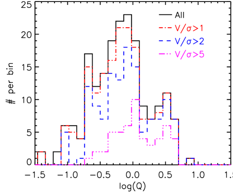
Figure 9: The distribution of Toomre Q for all galaxies in our sample that are classed as rotationally supported. We also sub-divide the sample by the ratio of rotational velocity to velocity dispersion (V / $\sigma$), with V / $\sigma>$ 1, 2 and 5. The full range of Q for the whole sample is $Q$ = 0.08–5.6, but with increasing V / $\sigma$, the median Toomre Q also increases to Q = 0.80 $\pm$ 0.10, Q = 0.80 $\pm$ 0.10, Q = 0.90 $\pm$ 0.08 and Q = 1.30 $\pm$ 0.16 for the full sample to V / $\sigma>$ 1, 2 and 5 respectively.

Nevertheless, this observable provides a crude, but common way to classify the stability of the gas in a disk and this will be important in comparison with the angular momentum. For example, in local galaxies Cortese et al. (2016) (using SAMI) and Lagos et al. (2016) (using the eagle galaxy formation model) show that the disk stability and galaxy spin, $\lambda_{\rm R}$ (as defined in Emsellem et al., 2007) are strongly correlated with $V$ / $\sigma$ and define a continious sequence in the specific angular momentum–stellar mass plane, where galaxies with high specific angular momentum are the most stable with high $V$ / $\sigma$ and $\lambda_{\rm R}$. Moreover, Stevens et al. (2016) (see also Obreschkow et al., 2015) suggest that specific angular momentum plays a defining role in defining the disk stability. We will return this in § 4.

4 Discussion

Observations of the sizes and rotational velocities of local spiral galaxies have suggested that $\sim$ 50% of the initial specific angular momentum of the baryons within dark matter halos must be lost due to viscous angular momentum redistribution and selective gas losses which occur as the galaxy forms and evolves.

In Fig. 8 we plot the specific angular momentum versus stellar mass for the high-redshift galaxies in our MUSE and KMOS sample. In this figure, we split the sample by their dynamics according to their ratio of $V$ / $\sigma$ (although we also highlight the galaxies whose dynamics most obviously display rotational support). We include the unresolved galaxies from our sample using the limits on their sizes and velocity dispersions (the latter to provide an estimate of the upper limit on $V_{\rm c}$). In this figure, we also include the distribution (and median+scatter) at $z$ = 0 and $z\sim$ 1 from the eagle simulation.

Since there is considerable scatter in the data we bin the specific angular momentum in stellar mass bins (using bins with d log₁₀(M_⋆) = 0.3 dex) and overlay the median (and scatter in the distribution) in Fig. 8. Up to a stellar mass of $\sim$ 10^10.5 M_⊙, the high-redshift galaxies follow a similar scaling between stellar mass and specific angular momentum as seen in local galaxies (see also Contini et al., 2015). Fitting the data over the stellar mass range M_⋆ = 10^8.5–10^11.5 M_⊙, we derive a scaling of $j_{\star}\propto$ M${}_{\star}^{\rm q}$ with $q$ = 0.6 $\pm$ 0.1. Although the scaling $j_{\star}\propto$ M${}_{\star}^{2/3}$ is generally seen in local galaxies, when galaxies are split by morphological type, the power-law index varies between $q$ = 0.7–1 (e.g. Cortese et al. 2016). However, the biggest difference between $z$ = 0 and $z$ = 1 is above a stellar mass of $M_{\star}\sim$ 10^10.5 M_⊙, where the specific angular momentum of galaxies at $z\sim$ 1 is 2.5 $\pm$ 0.5$\times$ lower than for comparably massive spiral galaxies at $z\sim$ 0, and there are no galaxies in our observation sample with specific angular momentum as high as those of local spirals.

First we note that this offset (and lack of galaxies with high specific angular momentum) does not appear to be driven by volume or selection effects which result in our observations missing high stellar mass, high $j_{\star}$ galaxies. For example, although the local galaxy sample from Romanowsky & Fall (2012) sample is dominated by local (D $<$ 180Mpc) high-mass, edge on spiral disks, the space density of star-forming galaxies with stellar mass $>$10¹¹ M_⊙ at $z\sim$ 1 is $\sim$ 1.6 $\times$ 10^-3 Mpc^-3 (Bundy et al., 2005). The volume probed by the MUSE and KMOS observations is $\sim$ 1.5 $\times$ 10⁴ Mpc³ (comoving) between $z$ = 0.4–1.2 and we expect $\sim$ 23 $\pm$ 4 such galaxies in our sample above this mass (and we detect 20). Thus, we do not appear to be missing a significant population of massive galaxies from our sample. At $z\sim$ 1, we are also sensitive to star formation rates as low as $\sim$ 4 M_⊙ yr^-1 (given our typical surface brightness limits and adopting a median reddening of $A_{\rm V}$ = 0.5). This is below the so-called “main-sequence” at this redshift since the star formation rate for a “main-sequence” galaxy with M_⋆ = 10¹¹ M_⊙ at $z$ = 1 is 100 M_⊙ yr^-1 (Wuyts et al., 2013).

What physical processes are likely to affect the specific angular momentum of baryonic disks at high-redshift (particularly those in galaxies with high stellar masses)? Due to cosmic expansion, a generic prediction of $\Lambda$CDM is that the relation between the mass and angular momentum of dark matter halos changes with time. In a simple, spherically symmetric halo the specific angular momentum, $j_{\rm h}$ = $J_{\rm h}$ / M_h should scale as $j_{\rm h}$ = M${}_{\rm h}^{2/3}(1+z)^{-1/2}$ (e.g.  Obreschkow et al., 2015) and if the ratio of the stellar-to-halo mass is independent of redshift, then the specific angular momentum of the baryons should scale as $j_{\star}\propto M_{\star}^{2/3}(1+z)^{-1/2}$. At $z\sim$ 1, this simple model predicts that the specific angular momentum of disks should be $\sqrt{2}$ lower than at $z$ = 0.

However, this ’closed-box’ model does not account for gas inflows or outflows, and cosmologically based models have suggested redshift evolution in $j_{\star}$ / M^2/3 can evolve as rapidly as (1+$z$)^-3/2 from $z\sim$ 1 to $z$ = 0 (although this redshift evolution is sensitive to the mass and star formation rate limits applied to the selection of the galaxies; e.g. Lagos et al. 2016). For example, applying our mass and star-formation rate limits to galaxies in the eagle model, galaxies at $z\sim$ 1 are predicted to have specific angular momentum which is 0.2 dex lower (or a factor $\sim$ 1.6$\times$) lower than comparably massive galaxies at $z$ = 0, although the most massive spirals at $z$ = 0 have specific angular momentum which is $\sim$ 3 times larger than any galaxies in our high-redshift sample.

The specific angular momentum of a galaxy can be increased or decreased depending on the evolution of the dark halo, the angular momentum and impact parameter of accreting material from the inter-galactic medium, and how the star-forming regions evolve within the ISM. For example, if the impact parameter of accreting material is comparable to the disk radius (as suggested in some models; e.g. Dekel et al. 2009), then the streams gradually increase the specific angular momentum of the disk with decreasing redshift as the gas accretes on to the outer disk. The specific angular momentum can be further increased if the massive, star-forming regions (clumps) that form within the ISM torque and migrate inwards (since angular momentum is transferred outwards). However, galaxy average specific angular momentum can also be decreased if outflows (associated with individual clumps) drive gas out of the disk, and outflows with mass loading factors $\gg$1 associated with individual star forming regions (clumps) have been observed in a number of high-redshift galaxies (e.g.  Genzel et al., 2011; Newman et al., 2012).

Since the galaxies in our sample span a range of redshifts, from $z\sim$ 0.3–1.7, to test how the specific angular momentum evolves with time, we split our sample in to four redshift bins. Whilst it has been instructive to normalise angular momentum by stellar mass ($j_{\star}$ = $J$ / $M_{\star}$), the stellar mass is an evolving quantity, and so we adopt the quantity $j_{\star}$ / $M_{\star}^{2/3}$ (or equivalently, $J$ / M${}_{\star}^{5/3}$) and in Fig. 10 we compare the evolution of $j_{\star}$ / M${}_{\star}^{2/3}$ for our sample with late- and early-types at $z$ = 0. This figure shows that there appears to be a trend of increasing specific angular momentum with decreasing redshift.

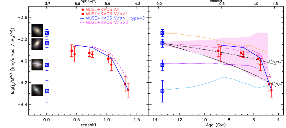
Figure 10: Left: Redshift evolution of the $j_{\star}$ / M${}_{\star}^{2/3}$ from $z$ = 0 to $z\sim$ 1.5. We split the $z$ = 0 galaxies from Romanowsky & Fall (2012) in to their types (from S0 to Sd). Data points and their error-bars in all of the observational points denote the bootstrap median and scatter in the distribution. Right: The average evolution of individual galaxies in the eagle simulation (observational data is the same as in the left panel). We identify all galaxies in eagle that have angular momentum consistent with late- and early-type galaxies at $z$ = 0 and use the merger trees to measure the ratio of $j_{\star}$ / M${}_{\star}^{2/3}$ of the main progenitor galaxy with redshift. We show the typical evolution and the scatter (68%) by the shaded region. In eagle, above $z\sim$ 1.5, the angular momentum of the model early- and late-types is similar, but below $z\sim$ 1.5, the ratio of $j_{\star}$ / M${}_{\star}^{2/3}$ grows by $\sim$ 60% due to a combination of gas accretion and outflows (which preferentially expel low angular momentum material). In comparison, the angular momentum of the galaxies which end up as early types at $z$ = 0 remains approximately constant over the same period. We also overlay a track of $j_{\star}$ / M${}_{\star}^{2/3}\propto$ (1 + $z$)^-n with $n$ = 0.5 and $n$ = 1.5. The former represents the evolution if the angular momentum grows linearly with time.

Before interpreting this plot in detail, first we note that Lagos et al. (2016) use eagle to show that the redshift evolution of $j_{\star}$ / M${}_{\star}^{2/3}$ is sensitive to the mass and star formation rate limits (see the “Active” versus “Passive” population in Fig. 12 of Lagos et al. 2016). To test whether our results are sensitive to selection effects (in particular the evolving mass limits may result in our observation missing low stellar mass galaxies at $z\sim$ 1 which are detectable at $z\sim$ 0.3), we select all of the galaxies from eagle between $z$ = 0.3–1.5 whose star-formation rates suggest [Oii] (or H$\alpha$) emission line fluxes (calculated using their star-formation rate, redshift and adopting a typical reddening of A_V = 0.5) are above $f_{\rm lim}$ = 1 $\times$ 10^-17 erg s^-1 cm^-2. This flux limit corresponds approximately to the flux limit of our survey. We then apply mass cuts of M_⋆ = 0.5, 5, and 20 $\times$ 10⁹ M_⊙ (which span the lower- median- and upper-quartiles of the stellar mass range in the observations). The stellar mass limits we applied to the eagle galaxies (which vary by a factor 40 from 0.5–20 $\times$ 10⁹ M_⊙), result in a change in the ratio of $j$ / M${}_{\star}^{2/3}$ of (a maximum of) 0.05 dex. Thus the trend we see in $j$ / M^2/3 with redshift does not appear to be driven by selection biases.

Thus, assuming the majority of the rotationally supported high-redshift galaxies in our sample continue to evolve towards the spirals at $z\sim$ 0, Fig. 10 suggests a change of $\Delta(j/M^{2/3})\sim$ 0.4 dex from $z\sim$ 1 to $z\sim$ 0. Equivalently, the evolution in $j_{\star}$ / M${}_{\star}^{2/3}$ is consistent with $j_{\star}$ / M${}_{\star}^{2/3}\propto(1+z)^{-n}$ with $n\sim$ $-$1. In the right-hand panel of Fig. 10, we plot the data in linear time and overlay this redshift evolution. The evolution of $j_{\star}$ / M${}_{\star}^{2/3}\propto(1+z)^{-1}$ is consistent with that predicted for massive galaxies in eagle (galaxies in halos with masses $M_{\rm halo}$ = 10^11.8-12.3 M_⊙; Lagos et al. 2016). In the figure, we also overlay tracks with $j_{\star}$ / M${}_{\star}^{2/3}\propto(1+z)^{-3/2}$ and $j_{\star}$ / M${}_{\star}^{2/3}\propto(1+z)^{-1/2}$ to show how the various predictions compare to the data.

Of course, the assumption that the rotationally supported “disks” at $z\sim$ 1 evolve in to the rotationally supported spirals at $z\sim$ 0 is difficult to test observationally. However the model does allow us to measure how the angular momentum of indivudual galaxies evolves with time. To test how the angular momentum of today’s spirals has evolved with time, and in particular what these evolved from at $z\sim$ 1, we identify all of the galaxies in eagle whose (final) $j_{\star}$ / M${}_{\star}^{2/3}$ is consistent with today’s early- and late-types ($j_{\star}$ / M${}^{2/3}_{\star}$ = $-$3.82 $\pm$ 0.05 and $-$4.02 $\pm$ 0.05 respectively) and trace the evolution of their angular momentum with redshift (using the main sub-halo progenitor in each case to trace their dynamics). We show these evolutionary tracks in Fig. 10. In the eagle simulation, early-type galaxies at $z$ = 0 have an approximately constant $j_{\star}$ / M${}_{\star}^{2/3}$ from $z\sim$ 1. This is similar to the findings of Lagos et al. (2016) who show that galaxies with mass-weighted ages $\mathrel{\raise 1.50696pt\hbox{$\scriptstyle>$}\kern-6.00006pt\lower 1.72218pt\hbox{{$\scriptstyle\sim$}}}$ 9 Gyr have constant $j_{\star}/M^{2/3}$ with redshift below $z\sim$ 2. In contrast, the model predicts that spiral galaxies at $z\sim$ 0 have gradually increased their specific angular momentum from high redshift, and indeed, for our observed sample, that the angular momentum of galaxies follows $j_{\star}$ / $M_{\star}^{2/3}\propto(1+z)^{-1}$ (see also Fig. 8). Thus, in the models, the specific angular momentum of todays spirals was $\sim$ 2.5$\times$ lower that at $z$ = 0. The increase in $j_{\star}$ / M${}_{\star}^{2/3}$ has been attributed to the age at which dark matter halos cease their expansion (their so-called “turnaround epoch”) and the fact that star forming gas at late times has high specific angular momentum which impacts the disk at large radii (e.g. see Fig. 13 of Lagos et al. 2016).

It is useful to investigate the relation between the angular momentum, stability of the disks and the star formation rate (or star formation surface density). As we discussed in § 3.9, the stability of a gas disk against clump formation is quantified by the Toomre parameter, $Q$. Recently, Obreschkow et al. (2015) suggested that the low angular momentum of high-redshift galaxies is the dominant driver of the formation of “clumps”, which hence leads to clumpy/disturbed mophologies and intense star formation. As the specific angular momentum increases with decreasing redshift, the disk-average average Toomre $Q$ becomes greater than unity and the disk becomes globally stable.

To test whether this is consistent with the galaxies in our sample, we select all the rotationally-supported galaxies from our MUSE and KMOS survey that have stellar masses greater than M_⋆ = 10¹⁰ M_⊙, and split the sample in to galaxies above and below $j_{\star}$ / M${}_{\star}^{2/3}$ = 10^2.5 km s^-1 kpc M${}_{\odot}^{-2/3}$ (we only consider galaxies above M_⋆ = 10¹⁰ M_⊙ since these are well resolved in our data). For these two sub-samples, we derive $Q$ = 1.10 $\pm$ 0.18 for the galaxies with the highest $j_{\star}$ / M${}_{\star}^{2/3}$ and $Q$ = 0.53 $\pm$ 0.22 for those galaxies with the lowest $j_{\star}$ / M${}_{\star}^{2/3}$. This is not a particularly surprising result since the angular momentum and Toomre $Q$ are both a strong function of rotational velocity and radius However, it is interesting to note that the average star formation rate and star formation surface densities of these two subsets of high and low $j_{\star}$ / M^2/3 are also markedly different. For the galaxies above the $j_{\star}$ / M^2/3 sequence at this mass, the star formation rates and star-formation surface densities are SFR = 8 $\pm$ 4 M_⊙ yr^-1 and $\Sigma_{\rm SFR}$ = 123 $\pm$ 23 M_⊙ yr^-1 kpc² respectively. In comparison, the galaxies below the sequence have higher rates, with SFR = 21 $\pm$ 4 M_⊙ yr^-1 and $\Sigma_{\rm SFR}$ = 206 $\pm$ 45 M_⊙ yr^-1 kpc² respectively. In this comparison, the star-formation rates are the most illustrative indication of the difference in sub-sample properties since they are independent of $j_{\star}$, stellar mass and size.

Since a large fraction of our sample have been observed usign HST, we can also investigate the morphologies of those galaxies above and below the specific angular momentum–stellar mass sequence. In Fig. 11 we show HST colour images of fourteen galaxies, seven each with specific angular momentum ($j_{\star}$) that are above or below the $j_{\star}$–M_⋆ sequence. We select galaxies for this plot which are matched in redshift and stellar mass (all have stellar masses $>$ 2 $\times$ 10⁹ M_⊙, with medians of log₁₀(M_⋆ / M_⋆) = 10.3 $\pm$ 0.4 and 10.2 $\pm$ 0.3 and $z$ = 0.78 $\pm$ 0.10 and 0.74 $\pm$ 0.11 respectively for the upper and lower rows). Whilst a full morphological analysis is beyond the scope of this paper, it appears from this plot that the galaxies with higher specific angular momentum (at fixed mass) are those with more established (smoother) disks. In contrast, the galaxies with lower angular momentum are those with morphologies that are either more compact, more disturbed morphologies and/or larger and brighter clumps.

Figure 11: HST colour images of fourteen galaxies from Fig. 8 whose specific angular momentum ($j_{\star}$) are below the $j_{\star}$–M_⋆ sequence (upper row) and below the $j_{\star}$–M_⋆ sequence (lower row). The galaxies shown in this figure all have stellar masses $>$ 2 $\times$ 10⁹ M_⊙, with similar stellar masses and redshift distributions (log₁₀(M_⋆ / M_⋆ = 10.3 $\pm$ 0.4 and 10.2 $\pm$ 0.3 and $z$ = 0.78 $\pm$ 0.10 and 0.74 $\pm$ 0.11 respectively for the upper and lower rows). The stellar masses and redshifts are given in the upper and lower left-hand corners respectively. The value in the lower-right hand corner of each image is the fractional offset from the $j_{\star}$–M_⋆ sequence in Fig. 8 (i.e. a value of 0.2 means that galaxy has a specific angular momentum that is 5$\times$ lower than the $j_{\star}$–$M_{\star}$ sequence given its stellar mass). These images demonstrate that galaxies with lower specific angular momentum (at fixed mass) are those with more disturbed morphologies and larger and brighter clumps (upper row), whilst the galaxies with high angular momentum are those with morphologies that more cloesly resemble spiral galaxies (lower row). The with low specific angular momentum are also dynamically unstable, with Toomre $Q$ = 0.53 $\pm$ 0.22 compared to those with high specific angular momentum which have Toomre $Q$ = 1.10 $\pm$ 0.18. Together, this demonstrates that the disk stability and morphology of the galaxies is strongly correlated with the angular momentum of the gas disk.

Taken together, these results suggest that at $z\sim$ 1, galaxies follow a similar scaling between mass and specific angular momentum as those at $z\sim$ 0. However, at high masses ($>$M_⋆ at $z\sim$ 1) star-forming galaxies have lower specific angular momentum (by a factor $\sim$ 2.5) than a mass matched sample at $z\sim$ 0, and we do not find any high-redshift galaxies with specific angular momentum as high as those in local spirals. From their Toomre stability and star formation surface densities, the most unstable disks have the lowest specific angular momentum, asymmetric morphologies and highest star formation rate surface densities (see also Obreschkow et al., 2015). Galaxies with higher specific angular momentum appear to be more stable, with smoother (disk-like) morphologies.

Finally, we calculate the distribution of baryonic spins for our sample. The spin typically refers to the fraction of centrifugal support for the halo. Both linear theory and N-body simulations have suggested that halos have spins that follow approximately log-normal distributions with average value $\lambda_{\rm DM}$ = 0.035 (Bett et al., 2007) (i.e. only $\sim$3.5% of the dynamical support of a halo is centrifugal, the rest comes from dispersion). To estimate how the disk and halo angular momentum are related, we calculate the spin of the disk, $\lambda$ as $\lambda$ = $\sqrt{2}$ / 0.1 $R_{\rm d}$ $H(z)$ / V(3 $R_{\rm d}$) where $H(z)$ = $H_{\rm 0}(\Omega_{\rm\Lambda,0}+\Omega_{\rm m,0}(1+z)^{3})^{0.5}$. This is the simplest approach that assumes the galaxy is embedded inside an isothermal spherical cold-dark matter halos (e.g.  White, 1984; Mo et al., 1998) which are truncated at the virial radius (Peebles 1969; see Burkert et al. 2015 for a discussion for the results from adopting more complex halo profiles). In Fig. 12 we plot the distribution of $\lambda\times$ ($j_{\rm d}$ / $j_{\rm DM}$) for our sample. If the initial halo and baryonic angular momentum are similar, i.e. $j_{\rm DM}\simeq j_{d}$, this quantity reflects the fraction of angular momentum lost during the formation of $z\sim$ 1 star-forming galaxies. In this figure, we split the sample in to four catagories: all galaxies with disk-like dynamics with V / $\sigma>$ 1, 2 and 5. We fit these distribution with a log-normal power-law distribution, deriving best-fit parameters in [$\lambda^{\prime},\sigma$] of [0.040 $\pm$ 0.002, 0.45 $\pm$ 0.05], [0.041 $\pm$ 0.002, 0.42 $\pm$ 0.05] and [0.068 $\pm$ 0.002, 0.50 $\pm$ 0.04] respectively.

Figure 12: The distribution of spin ($\lambda\times$ ($j_{\rm d}$ / $j_{\rm DM}$)) for the galaxies in our sample. We split the sample in to four catagories: All rotationally supported systems, and those with V / $\sigma>$ 1, 2 and 5. We fit the distribution of galaxies with V / $\sigma>$ 2 with a power-law relation to derive best-fit parameters $\lambda^{\prime}$ = 0.040 $\pm$ 0.002 and $\sigma$ = 0.045 $\pm$ 0.005.

An alternative approach (see also Harrison et al. 2017) is to assume the spin for the baryons of $\lambda^{\prime}$ = 0.035 and calculate the fraction of angular momentum that has been retained (assuming $j_{\rm DM}\simeq j_{d}$ initially). For the galaxies that appear to be rotationally supported with ratios of $V$ / $\sigma>$1, 2 and 5 we derive median values of $j_{\rm d}$ / $j_{\rm DM}\sim$ 1.18 $\pm$ 0.10, 0.95 $\pm$ 0.06 and 0.70 $\pm$ 0.05 (bootstrap errors). Since these spins are similar to the halo ($\lambda$ = 0.035) this suggests that the angular momentum of “rotationally supported” galaxies at $z\sim$ 1 broadly follows that expected from theoretical expectation from the halo, with most of the angular momentum retained during the (initial) collapse. Equivalently, for the galaxies with the highest ratio of $V$ / $\sigma$ (which are also those with the highest specific angular momentum and latest morphological types; see Fig. 11), the fraction of angular momentum retained must be $\mathrel{\raise 1.50696pt\hbox{$\scriptstyle>$}\kern-6.00006pt\lower 1.72218pt\hbox{{$\scriptstyle\sim$}}}$ 70%.

5 Conclusions

Exploiting MUSE and KMOS observations, we study the dynamics of 405 star-forming galaxies across the redshift range $z$ = 0.28–1.65, with a median redshift of $z$ = 0.84. From estimates of their stellar masses and star formation rates, our sample appear to be representative of the star-forming “main-sequence” from $z$ = 0.3–1.7, with ranges of SFR = 0.1–30 M_⊙ yr^-1 and M_⋆ = 10⁸–10¹¹ M_⊙.

Our main results are summarised as:

$\bullet$ From the dynamics and morphologies of the galaxies in the sample, 49 $\pm$ 4% appear to be rotationally supported; 24 $\pm$ 3% are unresolved; and only $\sim$ 5 $\pm$ 2% appear to be major mergers. The remainder appear to be irregular (or perhaps face-on) systems. Our estimate of the “disk” fraction in this sample is consistent with other dynamical studies over a similar redshift range which have also found that rotationally supported systems make up $\sim$ 40–70% of the star-forming population.

$\bullet$ We measure half light sizes of the galaxies in both the broad-band continuum images (using HST imaging in many cases) and in the nebular emission lines. The nebular emission line sizes are typically a factor of 1.18 $\pm$ 0.03 $\times$ larger than the continuum sizes. This is consistent with recent results from the 3-DHST survey which has also shown that the nebular emission from $\sim$ $L^{\star}$ star-forming galaxies at $z\sim$ 1 are systematically more extended than the stellar continuum.

$\bullet$ For those galaxies whose dynamics resemble rotationally supported systems, we simultaneously fit the imaging and dynamics with a disk + halo model to derive the best-fit structural parameters (such as disk inclination, position angle, [$x$ / $y$] center, disk mass, disk size, dark matter core radius and density). The dynamical and morphological major axes are typically misaligned by $\Delta$ PA = 9.5 $\pm$ 0.5^∘, which we attribute to the dynamical “settling” of the gas and stars as the disks evolve.

$\bullet$ We combine the inclination-corrected rotational velocities with the galaxy sizes and intrinsic velocity dispersions to investigate the global stability of the gas disks. For the galaxies that are classified as rotationally supported, we derive a median Toomre $Q$ of $Q$ = 0.80 $\pm$ 0.10. This is consistent with numerical models that predict that in high-redshift, gas rich galaxies the disks are maintained at the marginally stable threshold due to the feedback from stellar winds which arrest collapse (e.g.  Hopkins, 2012).

$\bullet$ We use the galaxy sizes, rotation speeds and stellar masses to investigate how the specific angular momentum of gas disks evolves with cosmic time. We show that the galaxies in our sample (which have a median redshift of $z$ = 0.84 $\pm$ 0.03) follow a similar scaling between stellar mass and specific angular momentum as local galaxies. Fitting the data over the stellar mass range M_⋆ = 10^8.5–10^11.5 M_⊙ suggests $j_{\star}\propto$ M${}_{\star}^{\rm q}$ with $q$ = 0.6 $\pm$ 0.1. However, at $z$ = 1, we do not find any galaxies with specific angular momentum as high as those of local spirals. Thus, the most massive star-forming disks at $z\sim$ 0 must have increased their specific angular momentum (by a factor $\sim$ 3) between $z\sim$ 1 and $z\sim$ 0.

$\bullet$ To account for the evolving stellar masses of galaxies, we measure the ratio of $j_{\star}$ / M${}_{\star}^{2/3}$ and split our observed sample in to four redshift bins between $z$ = 0.3 and $z$ = 1.5. For a star-formation selected (and mass limited) sample, we show that the specific angular momentum evolves with redshift as $j_{\star}\propto$ M${}_{\star}^{2/3}(1+z)^{-1}$, which is similar to that predicted by the latest numerical models, which also suggest that spiral galaxies at $z\sim$ 0 appear to have gradually accreted their specific angular momentum from high redshift (in contrast to “passive” galaxies at $z\sim$ 0 which, on average, have near constant specific angular momentum between $z\sim$ 0 and $z\sim$ 1).

$\bullet$ Combining the measurements of the angular momentum, star formation surface density and disk stability, we show that galaxies with stellar masses greater than M_⋆ = 10¹⁰ M_⊙ with the highest $j_{\star}$ / M${}_{\star}^{2/3}$ are the most stable, with disks with Toomre $Q$ = 1.20 $\pm$ 0.20, compared to $Q$ = 0.51 $\pm$ 0.17 for galaxies above and below $j_{\star}$ / M${}_{\star}^{2/3}$ = 10^2.5 km s^-1 kpc M${}_{\odot}^{-2/3}$ respectively. Since $j_{\star}$ and $Q$ are both functions of size and rotational velocity, we also measure the average star formation rate and star formation surface densities of these two subsets of high and low $j_{\star}$ / M^2/3 galaxies. These sub-samples are markedly different, with a median $\Sigma_{\rm SFR}$ = 123 $\pm$ 23 M_⊙ yr^-1 and $\Sigma_{\rm SFR}$ = 206 $\pm$ 45 M_⊙ yr^-1 for those galaxies above and below the fiducial $j_{\star}$ / M${}_{\star}^{2/3}$ relation respectively. In terms of star formation rates alone, there is a similar difference, with SFR = 8 $\pm$ 4 M_⊙ yr^-1 and SFR = 21 $\pm$ 4 M_⊙ yr^-1 above and below the sequence respectively.

$\bullet$ At a fixed mass, we show that galaxies with high specific angular momentum ($j_{\star}$) (i.e. those above the $j_{\star}$–M_⋆ ) relation are those with morphologies that more closely resemble spiral galaxies, with bigger bulges and smoother disks. In contrast, galaxies with lower specific angular momentum (at fixed mass) are those with more disturbed, asymmetric morphologies, larger and brighter clumps.

$\bullet$ Finally, we show that the distribution of spins for the rotationally supported galaxies in our sample is similar to that expected for the halos. For exampe, for galaxies that have disk like dynamics and $V$ / $\sigma>$ 2 we derive $\lambda^{\prime}$ = 0.040 $\pm$ 0.002 and $\sigma$ = 0.45 $\pm$ 0.05. This suggests that the angular momentum of “rotationally supported” galaxies at $z\sim$ 1 broadly follows that expected from theoretical expectation from the halo, with most of the angular momentum retained during the (initial) collapse.

Overall, our results show that star forming disks at $z\sim$ 1 have lower specific angular momentum than a stellar mass matched sample at $z\sim$ 0. At high redshift, the fraction of rotationally supported “disk” galaxies is high, yet most of these galaxies appear irregular/clumpy. This appears to be due to the high low angular momentum which results in globally unstable, turbulent systems. Indeed, specific angular momentum appears to play a major role in defining the disk stability, star formation surface densities and morphology. As the specific angular momentum of growing disks increases below $z\sim$ 1, the galaxy disks must evolve from globally unstable clumpy, turbulent systems in to stable, flat regular spirals.

Table 2: Galaxy Properties

ID	RA	Dec	$z$	$V_{\rm AB}$	$K_{\rm AB}$	$f_{\rm neb}$	$r_{\rm h,\star}$	$r_{\rm h,neb}$	$M_{\rm H}$	log($\frac{M_{\star}}{M_{\odot}}$)	$\sigma_{\rm gal}$	$\sigma_{\rm int}$	$V$(3 Rd)	$i$	$A_{\rm V}$	$j_{\star}$	SFR	Class
	(J2000)						[$"$]	[$"$]			[km s-1]	[km s-1]	[km s-1]			[km s-1kpc]	[M⊙yr-1]
COSMOS-K1-1	09:59:40.603	+02:21:04.15	1.6350	24.98	22.53	5.7	0.41 $\pm$ 0.10	0.45 $\pm$ 0.15	-22.25	10.48	131 $\pm$ 3	46 $\pm$ 3	16 $\pm$ 7	22 $\pm$ 22	0.2	66 $\pm$ 41	11	D
COSMOS-K1-2	09:59:31.589	+02:19:05.47	1.6164	23.70	20.63	5.1	0.18 $\pm$ 0.01	0.24 $\pm$ 0.05	-24.46	11.40	176 $\pm$ 3	…	…	…	0.6	345 $\pm$ 6	16	C
COSMOS-K1-3	09:59:33.994	+02:20:54.58	1.5240	23.90	21.73	5.0	0.57 $\pm$ 0.13	0.68 $\pm$ 0.13	-22.85	10.57	123 $\pm$ 3	38 $\pm$ 3	206 $\pm$ 30	37 $\pm$ 10	0.4	1171 $\pm$ 463	10	D
COSMOS-K1-4	09:59:28.339	+02:19:50.53	1.4855	21.02	19.96	86.9	0.08 $\pm$ 0.05	0.30 $\pm$ 0.26	-24.51	11.09	580 $\pm$ 3	…	…	…	0.0	…	100	I
COSMOS-K1-10	09:59:30.902	+02:18:53.04	1.5489	24.06	21.60	15.4	0.20 $\pm$ 0.02	0.04 $\pm$ 0.05	-23.21	10.72	159 $\pm$ 3	…	…	…	0.6	344 $\pm$ 5	44	C

The full table is given in the online version of this paper. The first five rows are shown here for their content. Notes: $f_{\rm neb}$ denotes the nebular emission line flux ([Oii] in the case of MUSE and H$\alpha$ for KMOS) in units of 10^-17 erg cm^-2 s^-1. $r_{\rm h,\star}$ and $r_{\rm h,neb}$ are the (deconvolved) continuum and nebular emission half light radii respectively. $\sigma_{\rm neb}$ denotes the galaxy-integrated velocity dispersion as measured from the one-dimensional spectrum. $\sigma_{\rm int}$ denotes the average intrinsic velocity dispersion within the galaxy (after correcting for beam smearing effects). $V$(3 R_d) is the observed velocity at 3 R_d. $i$ is the disk inclination. SFR is measured from the [Oii] flux with SFR = 0.8 $\times$ 10^-41 L_[OII] erg s^-1 and correcting for dust reddenning using the Calzetti redenning law.

References

- Bacon et al. (2010) Bacon, R., Accardo, M., Adjali, L., Anwand, H., Bauer, S., Biswas, I., Blaizot, J., & et al., B. 2010, in Proceedings of SPIE, Vol. 7735, Ground-based and Airborne Instrumentation for Astronomy III, 773508
- Bacon et al. (2015) Bacon, R., Brinchmann, J., Richard, J., Contini, T., Drake, A., Franx, M., Tacchella, S., & Vernet, J. et al. 2015, A&AP, 575, A75
- Barnes & Efstathiou (1987) Barnes, J. & Efstathiou, G. 1987, ApJ, 319, 575
- Bell et al. (2004) Bell, E. F., McIntosh, D. H., Barden, M., Wolf, C., Caldwell, J. A. R., Rix, H.-W., Beckwith, S. V. W., & Borch, A. et al. 2004, ApJL, 600, L11
- Bertin & Arnouts (1996) Bertin, E. & Arnouts, S. 1996, AAPS, 117, 393
- Bertola & Capaccioli (1975) Bertola, F. & Capaccioli, M. 1975, ApJ, 200, 439
- Bett et al. (2007) Bett, P., Eke, V., Frenk, C. S., Jenkins, A., Helly, J., & Navarro, J. 2007, MNRAS, 376, 215
- Bolzonella et al. (2000) Bolzonella, M., Miralles, J.-M., & Pelló, R. 2000, A&AP, 363, 476
- Brammer et al. (2008) Brammer, G. B., van Dokkum, P. G., & Coppi, P. 2008, ApJ, 686, 1503
- Bruce et al. (2014) Bruce, V. A., Dunlop, J. S., McLure, R. J., Cirasuolo, M., Buitrago, F., Bowler, R. A. A., Targett, T. A., & Bell, E. F. et al. 2014, MNRAS, 444, 1660
- Buitrago et al. (2013) Buitrago, F., Trujillo, I., Conselice, C. J., & Häußler, B. 2013, MNRAS, 428, 1460
- Bundy et al. (2005) Bundy, K., Ellis, R. S., & Conselice, C. J. 2005, ApJ, 625, 621
- Burkert (1995) Burkert, A. 1995, ApJL, 447, L25
- Burkert (2009) Burkert, A. 2009, in Astronomical Society of the Pacific Conference Series, Vol. 419, Galaxy Evolution: Emerging Insights and Future Challenges, ed. S. Jogee, I. Marinova, L. Hao, & G. A. Blanc, 3
- Burkert et al. (2015) Burkert, A., Förster Schreiber, N. M., Genzel, R., Lang, P., Tacconi, L. J., Wisnioski, E., Wuyts, S., & Bandara, K. et al. 2015, ArXiv
- Calzetti et al. (2000) Calzetti, D., Armus, L., Bohlin, R. C., Kinney, A. L., Koornneef, J., & Storchi-Bergmann, T. 2000, ApJ, 533, 682
- Catelan & Theuns (1996) Catelan, P. & Theuns, T. 1996, MNRAS, 282, 436
- Ceverino et al. (2010) Ceverino, D., Dekel, A., & Bournaud, F. 2010, MNRAS, 404, 2151
- Ciardullo et al. (2013) Ciardullo, R., Gronwall, C., Adams, J. J., Blanc, G. A., Gebhardt, K., Finkelstein, S. L., Jogee, S., Hill, G. J., Drory, N., Hopp, U., Schneider, D. P., Zeimann, G. R., & Dalton, G. B. 2013, ApJ, 769, 83
- Cole & Lacey (1996) Cole, S. & Lacey, C. 1996, MNRAS, 281, 716
- Conselice et al. (2011) Conselice, C. J., Bluck, A. F. L., Ravindranath, S., Mortlock, A., Koekemoer, A. M., Buitrago, F., Grützbauch, R., & Penny, S. J. 2011, MNRAS, 417, 2770
- Contini et al. (2015) Contini, T., Epinat, B., Bouché, N., Brinchmann, J., Boogaard, L. A., Ventou, E., Bacon, R., & Richard, J. et al. 2015, ArXiv e-prints
- Courteau (1997) Courteau, S. 1997, AJ, 114, 2402
- Crain et al. (2015) Crain, R. A., Schaye, J., Bower, R. G., Furlong, M., Schaller, M., Theuns, T., Dalla Vecchia, C., & Frenk, C. S. 2015, ArXiv e-prints
- Danovich et al. (2015) Danovich, M., Dekel, A., Hahn, O., Ceverino, D., & Primack, J. 2015, MNRAS, 449, 2087
- Dekel et al. (2009) Dekel, A., Sari, R., & Ceverino, D. 2009, ApJ, 703, 785
- Emsellem et al. (2007) Emsellem, E., Cappellari, M., Krajnović, D., van de Ven, G., Bacon, R., Bureau, M., Davies, R. L., & de Zeeuw, P, et al. 2007, MNRAS, 379, 401
- Epinat et al. (2012) Epinat, B., Tasca, L., Amram, P., Contini, T., Le Fèvre, O., Queyrel, J., Vergani, D., Garilli, B., Kissler-Patig, M., Moultaka, J., Paioro, L., Tresse, L., Bournaud, F., López-Sanjuan, C., & Perret, V. 2012, A&AP, 539, A92
- Fall (1983) Fall, S. M. 1983, in IAU Symposium, Vol. 100, Internal Kinematics and Dynamics of Galaxies, ed. E. Athanassoula, 391–398
- Fall & Romanowsky (2013) Fall, S. M. & Romanowsky, A. J. 2013, ApJL, 769, L26
- Ferguson et al. (2004) Ferguson, H. C., Dickinson, M., Giavalisco, M., Kretchmer, C., Ravindranath, S., Idzi, R., Taylor, E., Conselice, C. J., Fall, S. M., Gardner, J. P., Livio, M., Madau, P., Moustakas, L. A., Papovich, C. M., Somerville, R. S., Spinrad, H., & Stern, D. 2004, ApJL, 600, L107
- Förster Schreiber et al. (2009) Förster Schreiber, N. M., Genzel, R., Bouché, N., Cresci, G., Davies, R., Buschkamp, P., Shapiro, K., & Tacconi, L. J.. et al. 2009, ApJ, 706, 1364
- Franx et al. (1991) Franx, M., Illingworth, G., & de Zeeuw, T. 1991, ApJ, 383, 112
- Freeman (1970) Freeman, K. C. 1970, ApJ, 160, 811
- Furlong et al. (2015) Furlong, M., Bower, R. G., Theuns, T., Schaye, J., Crain, R. A., Schaller, M., Dalla Vecchia, C., Frenk, C. S., McCarthy, I. G., Helly, J., Jenkins, A., & Rosas-Guevara, Y. M. 2015, MNRAS, 450, 4486
- Gallagher & Hunter (1984) Gallagher, III, J. S. & Hunter, D. A. 1984, ARAA, 22, 37
- Geach et al. (2008) Geach, J. E., Smail, I., Best, P. N., Kurk, J., Casali, M., Ivison, R. J., & Coppin, K. 2008, MNRAS, 388, 1473
- Genel et al. (2015) Genel, S., Fall, S. M., Hernquist, L., Vogelsberger, M., Snyder, G. F., Rodriguez-Gomez, V., Sijacki, D., & Springel, V. 2015, ApJL, 804, L40
- Genzel et al. (2011) Genzel, R., Newman, S., Jones, T., Förster Schreiber, N. M., Shapiro, K., Genel, S., Lilly, S. J., & Renzini, A. et al. 2011, ApJ, 733, 101
- Giavalisco et al. (1996) Giavalisco, M., Steidel, C. C., & Macchetto, F. D. 1996, ApJ, 470, 189
- Gnerucci et al. (2011) Gnerucci, A., Marconi, A., Cresci, G., Maiolino, R., Mannucci, F., Calura, F., Cimatti, A., & Cocchia, F. et al. 2011, A&AP, 528, A88
- Guo et al. (2009) Guo, Y., McIntosh, D. H., Mo, H. J., Katz, N., van den Bosch, F. C., Weinberg, M., Weinmann, S. M., Pasquali, A., & Yang, X. 2009, MNRAS, 398, 1129
- Harrison et al. (2017) Harrison, C. M., Johnson, H. L., Swinbank, A. M., Stott, J. P., Bower, R. G., Smail, I., Tiley, A. L., & Bunker, A. J. et al. 2017, ArXiv e-prints
- Hopkins (2012) Hopkins, P. F. 2012, MNRAS, 423, 2016
- Husband et al. (2015) Husband, K., Bremer, M. N., Stanway, E. R., & Lehnert, M. D. 2015, MNRAS, 452, 2388
- Kennicutt (1998) Kennicutt, Jr., R. C. 1998, ApJ, 498, 541
- Khostovan et al. (2015) Khostovan, A. A., Sobral, D., Mobasher, B., Best, P. N., Smail, I., Stott, J. P., Hemmati, S., & Nayyeri, H. 2015, ArXiv e-prints
- Kriek et al. (2009) Kriek, M., van Dokkum, P. G., Labbé, I., Franx, M., Illingworth, G. D., Marchesini, D., & Quadri, R. F. 2009, ApJ, 700, 221
- Lagos et al. (2016) Lagos, C. d. P., Theuns, T., Stevens, A. R. H., Cortese, L., Padilla, N. D., Davis, T. A., Contreras, S., & Croton, D. 2016, ArXiv:1609.01739
- Law et al. (2009) Law, D. R., Steidel, C. C., Erb, D. K., Larkin, J. E., Pettini, M., Shapley, A. E., & Wright, S. A. 2009, ApJ, 697, 2057
- Leitherer et al. (1999) Leitherer, C., Schaerer, D., Goldader, J. D., Delgado, R. M. G., Robert, C., Kune, D. F., de Mello, D. F., Devost, D., & Heckman, T. M. 1999, APJS, 123, 3
- Ly et al. (2007) Ly, C., Malkan, M. A., Kashikawa, N., Shimasaku, K., Doi, M., Nagao, T., Iye, M., Kodama, T., Morokuma, T., & Motohara, K. 2007, ApJ, 657, 738
- Mo et al. (1998) Mo, H. J., Mao, S., & White, S. D. M. 1998, MNRAS, 295, 319
- Morishita et al. (2014) Morishita, T., Ichikawa, T., & Kajisawa, M. 2014, ApJ, 785, 18
- Mortlock et al. (2013) Mortlock, A., Conselice, C. J., Hartley, W. G., Ownsworth, J. R., Lani, C., Bluck, A. F. L., Almaini, O., & Duncan, K. et al. 2013, MNRAS, 433, 1185
- Muzzin et al. (2013) Muzzin, A., Marchesini, D., Stefanon, M., Franx, M., Milvang-Jensen, B., Dunlop, J. S., Fynbo, J. P. U., Brammer, G., Labbé, I., & van Dokkum, P. 2013, APJS, 206, 8
- Navarro et al. (1997) Navarro, J. F., Frenk, C. S., & White, S. D. M. 1997, ApJ, 490, 493
- Nelson et al. (2015) Nelson, E. J., van Dokkum, P. G., Förster Schreiber, N. M., Franx, M., Brammer, G. B., Momcheva, I. G., Wuyts, S., & Whitaker, K. E. e. a. 2015, ArXiv e-prints
- Newman et al. (2012) Newman, S. F., Genzel, R., Förster-Schreiber, N. M., Shapiro Griffin, K., Mancini, C., Lilly, S. J., Renzini, A., & Bouché, N. et al. 2012, ApJ, 761, 43
- Obreschkow & Glazebrook (2014) Obreschkow, D. & Glazebrook, K. 2014, ApJ, 784, 26
- Obreschkow et al. (2015) Obreschkow, D., Glazebrook, K., Bassett, R., Fisher, D. B., Abraham, R. G., Wisnioski, E., & Green, A. W. et al. 2015, ApJ, 815, 97
- Oesch et al. (2010) Oesch, P. A., Carollo, C. M., Feldmann, R., Hahn, O., Lilly, S. J., Sargent, M. T., Scarlata, C., & Aller, et al. 2010, ApJL, 714, L47
- Peebles (1969) Peebles, P. J. E. 1969, ApJ, 155, 393
- Peng et al. (2002) Peng, C. Y., Ho, L. C., Impey, C. D., & Rix, H.-W. 2002, AJ, 124, 266
- Persic & Salucci (1988) Persic, M. & Salucci, P. 1988, MNRAS, 234, 131
- Puech et al. (2008) Puech, M., Flores, H., Hammer, F., Yang, Y., Neichel, B., Lehnert, M., Chemin, L., & Nesvadba, N. et al. 2008, A&AP, 484, 173
- Richard et al. (2015) Richard, J., Patricio, V., Martinez, J., Bacon, R., Clément, B., Weilbacher, P., Soto, K., & Wisotzki, L. et al. 2015, MNRAS, 446, L16
- Roberts (1963) Roberts, M. S. 1963, ARAA, 1, 149
- Romanowsky & Fall (2012) Romanowsky, A. J. & Fall, S. M. 2012, APJS, 203, 17
- Salucci & Burkert (2000) Salucci, P. & Burkert, A. 2000, ApJL, 537, L9
- Sandage (1986) Sandage, A. 1986, A&AP, 161, 89
- Sandage et al. (1970) Sandage, A., Freeman, K. C., & Stokes, N. R. 1970, ApJ, 160, 831
- Schaller et al. (2015) Schaller, M., Frenk, C. S., Bower, R. G., Theuns, T., Trayford, J., Crain, R. A., Furlong, M., Schaye, J., Dalla Vecchia, C., & McCarthy, I. G. 2015, MNRAS, 452, 343
- Schaye et al. (2015) Schaye, J., Crain, R. A., Bower, R. G., Furlong, M., Schaller, M., Theuns, T., Dalla Vecchia, C., & Frenk, C. S. et al. 2015, MNRAS, 446, 521
- Sharples et al. (2004) Sharples, R. M., Bender, R., Lehnert, M. D., Ramsay Howat, S. K., Bremer, M. N., Davies, R. L., Genzel, R., & Hofmann, R. 2004, in Ground-based Instrumentation for Astronomy. Edited by Alan F. M. Moorwood and Iye Masanori. Proceedings of the SPIE, Volume 5492, pp. 1179-1186 (2004)., ed. A. F. M. Moorwood & M. Iye, 1179–1186
- Sobral et al. (2009) Sobral, D., Best, P. N., Geach, J. E., Smail, I., Kurk, J., Cirasuolo, M., Casali, M., & Ivison, R. J. et al. 2009, MNRAS, 398, 75
- Sobral et al. (2015) Sobral, D., Matthee, J., Best, P. N., Smail, I., Khostovan, A. A., Milvang-Jensen, B., Kim, J.-W., Stott, J., Calhau, J., Nayyeri, H., & Mobasher, B. 2015, MNRAS, 451, 2303
- Sobral et al. (2013a) Sobral, D., Smail, I., Best, P. N., Geach, J. E., Matsuda, Y., Stott, J. P., Cirasuolo, M., & Kurk, J. 2013a, MNRAS, 428, 1128
- Sobral et al. (2013b) Sobral, D., Swinbank, A. M., Stott, J. P., Matthee, J., Bower, R. G., Smail, I., Best, P., Geach, J. E., & Sharples, R. M. 2013b, ApJ, 779, 139
- Steinmetz & Bartelmann (1995) Steinmetz, M. & Bartelmann, M. 1995, MNRAS, 272, 570
- Stott et al. (2014) Stott, J. P., Sobral, D., Swinbank, A. M., Smail, I., Bower, R., Best, P. N., Sharples, R. M., Geach, J. E., & Matthee, J. 2014, ArXiv e-prints
- Stott et al. (2016) Stott, J. P., Swinbank, A. M., Johnson, H. L., Tiley, A., Magdis, G., Bower, R., Bunker, A. J., & Harrison, C. M. et al. 2016, MNRAS, 457, 1888
- Toomre (1964) Toomre, A. 1964, ApJ, 139, 1217
- Trayford et al. (2015) Trayford, J. W., Theuns, T., Bower, R. G., Schaye, J., Furlong, M., Schaller, M., Frenk, C. S., Crain, R. A., Dalla Vecchia, C., & McCarthy, I. G. 2015, MNRAS, 452, 2879
- van der Wel et al. (2014) van der Wel, A., Franx, M., van Dokkum, P. G., Skelton, R. E., Momcheva, I. G., Whitaker, K. E., Brammer, G. B., & Bell, E. F. et al. 2014, ApJ, 788, 28
- Walter et al. (2008) Walter, F., Brinks, E., de Blok, W. J. G., Bigiel, F., Kennicutt, Jr., R. C., Thornley, M. D., & Leroy, A. 2008, AJ, 136, 2563
- White (1984) White, S. D. M. 1984, ApJ, 286, 38
- Wisnioski et al. (2015) Wisnioski, E., Förster Schreiber, N. M., Wuyts, S., Wuyts, E., Bandara, K., Wilman, D., Genzel, R., & Bender, R. e. a. 2015, ApJ, 799, 209
- Wuyts et al. (2013) Wuyts, S., Förster Schreiber, N. M., Nelson, E. J., van Dokkum, P. G., Brammer, G., Chang, Y.-Y., Faber, S. M., & Ferguson, H. C. et al. 2013, ApJ, 779, 135
- Zavala et al. (2016) Zavala, J., Frenk, C. S., Bower, R., Schaye, J., Theuns, T., Crain, R. A., Trayford, J. W., Schaller, M., & Furlong, M. 2016, MNRAS