Characterization and modeling of contamination for Lyman break galaxy samples at high redshift

Abstract

The selection of high redshift sources from broad-band photometry using the Lyman-break galaxy (LBG) technique is a well established methodology, but the characterization of its contamination for the faintest sources is still incomplete. We use the optical and near-IR data from four (ultra)deep Hubble Space Telescope legacy fields to investigate the contamination fraction of LBG samples at $z\sim 5-8$ selected using a colour-colour method. Our approach is based on characterizing the number count distribution of interloper sources, that is galaxies with colors similar to those of LBGs, but showing detection at wavelengths shorter than the spectral break. Without sufficient sensitivity at bluer wavelengths, a subset of interlopers may not be properly classified, and contaminate the LBG selection. The surface density of interlopers in the sky gets steeper with increasing redshift of LBG selections. Since the intrinsic number of dropouts decreases significantly with increasing redshift, this implies increasing contamination from misclassified interlopers with increasing redshift, primarily by intermediate redshift sources with unremarkable properties (intermediate ages, lack of ongoing star formation and low/moderate dust content). Using Monte Carlo simulations, we estimate that the CANDELS deep data have contamination induced by photometric scatter increasing from $\sim 2\%$ at $z\sim 5$ to $\sim 6\%$ at $z\sim 8$ for a typical dropout color $\geq 1$ mag, with contamination naturally decreasing for a more stringent dropout selection. Contaminants are expected to be located preferentially near the detection limit of surveys, ranging from 0.1 to 0.4 contaminants per arcmin² at $J_{\rm 125}\,$=30, depending on the field considered. This analysis suggests that the impact of contamination in future studies of $z>10$ galaxies needs to be carefully considered.

1. Introduction

The Lyman-break technique, first proposed by Steidel et al. (1996), transformed the identification of reliable samples of galaxy candidates at high-redshift from broad-band imaging, and it is now routinely used to study galaxy formation and evolution as early as $500$ Myr after the Big Bang, at redshift $z\sim 10$ (e.g., see Coe et al. 2015; Bouwens et al. 2015; McLeod et al. 2016; Oesch et al. 2016). While one could consider selecting high redshift samples based on the best-fit photometric redshift or redshift likelihood contours (e.g., McLure et al., 2010; Finkelstein et al., 2012; Bradley et al., 2014), Lyman break selection procedures utilising cuts in colour space can be simpler to apply and offer a slight advantage in terms of operational transparency. This makes such a selection procedure easier to reproduce by both theorists and observers, as follow-up studies by Shimizu et al. (2014); Lorenzoni et al. (2013); Schenker et al. (2013) show.

The idea of the method rests on the identification of the strong spectral break introduced by neutral hydrogen atoms along the line of sight at wavelengths shorter than Lyman-$\alpha$ (1216 Å rest-frame). Thus, to identify probable sources at high redshift with high confidence, the Lyman-break selection typically resorts to three crucial ingredients: (1) color information from two adjacent passbands to locate the wavelength location and measure the amplitude of the break, (2) color information red-ward of the break to characterize the intrinsic color of the source, and (3) evidence that sources have no flux blueward of the break.

Many studies have used different color selections, also depending on the availability of the photometric bands (e.g. Giavalisco et al., 2004; Bouwens et al., 2007; Castellano et al., 2012; Bradley et al., 2012; Oesch et al., 2012, 2014; Bouwens et al., 2012a, 2015, to cite a few), showing how different choices can still lead to comparable results and assessing the strength of the method.

The Lyman-break technique has been applied very successfully to build large samples of galaxies, especially from Hubble Space Telescope (HST) imaging (e.g. more than 10000 sources identified at $3.5\lesssim z\lesssim 11$ from HST legacy fields to date; see Bouwens et al. 2015). Also, substantial spectroscopic follow-up work has shown that samples are generally reliable, and that contamination from sources with similar colors but different redshift is generally under control (Steidel et al., 1999; Bunker et al., 2003; Malhotra et al., 2005; Dow-Hygelund et al., 2007; Popesso et al., 2009; Vanzella et al., 2009; Stark et al., 2010). Nonetheless, photometrically defined samples are intrinsically affected by contamination. While this possibility is universally acknowledged in the literature and specific studies estimate the contamination rate of the samples presented (e.g. Su et al. 2011; Pirzkal et al. 2013; Bouwens et al. 2015), surprisingly few studies have been devoted to a detailed characterization of the contamination rate and of its dependence on survey parameters and redshift of the galaxy population. Potential classes of contaminants that have been identified include stellar sources, low redshift galaxies with prominent 4000 Å/Balmer breaks and dust, extreme emission line galaxies, time-variable sources such as Supernovae, with the first two classes of objects representing the major risks (Stanway et al., 2008; Atek et al., 2011; Bowler et al., 2012).

Dwarf stars have similar colors to high-redshift galaxies because of their low surface temperatures, and can thus enter dropout samples, especially at $z\geq 7$ in data that lack sufficient angular resolution to discriminate point sources from extended light profiles (Stanway et al., 2003; Bouwens et al., 2006; Ouchi et al., 2009; Tilvi et al., 2013; Wilkins et al., 2014). At these redshifts, very low temperatures stars (sub-types M, L, T and Y) result in sources that are intrinsically faint, and spectra in which the continuum is interrupted may show large breaks across narrow-wavelength ranges, or in which the flux peaks in narrow regions. While deep medium-band observations are efficient in identifying these stellar contaminants in seeing-limited ground-based observations (Wilkins et al., 2014), HST imaging is generally effective in identifying stellar objects that are detected at signal-to-noise $S/N\gtrsim 10$ (Finkelstein et al., 2010; Bouwens et al., 2011b). In addition, we note that at $z>9$, the contamination from stars is negligible, since there are essentially no observed stars with spectral energy distributions (SEDs) that peak at $>1.4\mu m$ and are undetectable in the optical for typical HST surveys (e.g. Oesch et al., 2014).

The main source of contamination for space-based surveys is thus that of low/intermediate redshift galaxies that have a deep break around 4000 Å rest-frame. The nature of these contaminants has not been investigated in detail, but likely they are low-mass, moderate-age, Balmer break galaxies at $z\sim 1-3$ (Wilkins et al., 2010; Hayes et al., 2012), possibly with strong emission lines that contribute, or even dominate, the flux redward of the spectral break (van der Wel et al., 2011; Atek et al., 2011). To effectively discriminate between the high-$z$ Lyman-break and the 4000 Å/Balmer break, Stanway et al. (2008) recommend using a set of non-overlapping, but adjacent, filters, so that a clear color cut can be imposed on the selection. Another key requirement to build a clean sample is the availability of very deep observations blueward of the spectral break, to distinguish between a true non-detection for an high-$z$ object, and a faint continuum for an interloper (Bouwens et al., 2015).

The goal of this paper is to focus on this class of intermediate redshift interlopers, and to empirically quantify their impact on high-$z$ Lyman-break galaxy (LBG) samples selected via a colour-cut method and characterize how their incidence varies with depth and adopted selection cut. For this, we resort to the optical and near-infrared imaging on the GOODS South deep, GOODS North wide fields observed by the CANDLES program (Grogin et al., 2011) and the XDF (Illingworth et al., 2013) and HUDF09-2 (Bouwens et al., 2012b) fields. These datasets provide us high-quality multi-wavelength observations over different areas of the sky (from $\sim 4.7$ arcmin² to $\sim 64.5$ arcmin²). Specifically, we focus on LBG samples from $z\sim 5$ to $z\sim 8$, and investigate the population of galaxies that satisfy the color-color requirements to be included in the LBG selection based on imaging at wavelengths starting from the spectral break, but show a clear detection in bluer filters. We define this class of objects as interlopers, and characterize (1) their surface density in the sky depending on luminosity and on the redshift of the dropout selection; (2) the likelihood that fainter counterparts of the known population of interlopers enter a LBG sample because of lack of sufficiently deep imaging in the blue. We define this population as contaminants.

The results of our analysis, based on some of the deepest Hubble observations available, have multiple applications. In particular, they find applications to the estimation of the contamination rate of other surveys, which may lack the multi-wavelength, multi-observatory coverage, such as random pointings and/or parallel observations (e.g. see Trenti et al. 2011, 2012; Bradley et al. 2012; Schmidt et al. 2014; Calvi et al. 2016). Another important application includes planning and optimization of future observations (e.g., see Mason et al. 2015 for JWST and WFIRST surveys at high-$z$).

This paper is organized as follows: in Section 2 we introduce our dataset and construct the samples of dropouts and interlopers. In Section 3 we analyze and discuss the properties of the contaminants and the expected impact on LBG samples. In Section 4 we discuss how results depend on the selection criteria. We summarize and conclude in Section 5. Throughout the paper, we assume $\Omega_{0}=0.3$, $\Omega_{\Lambda}=0.7$, and $H_{0}=70\,km\,s^{-1}\,Mpc^{-1}$. All magnitudes are in the AB system (Oke & Gunn, 1983).

2. Dataset and sample selection

We base our analysis on four different samples, in order to test how results change with the field used for selection. We use the CANDELS/GOODS South deep (GSd) and CANDELS/GOODS North wide (GNw) imaging (Grogin et al., 2011), the entire XDF data set (Illingworth et al., 2013) and the HUDF09-2 (Bouwens et al., 2012b). A summary of all the data sets used in the present study is provided in Table 1, along with the covered area and the 5$\sigma$ depths. The latter are drawn from Bouwens et al. (2015) and are based on the median uncertainties in the total fluxes (after correction to total), as found for the faintest 20% of sources in the catalog. As discussed by Bouwens et al. (2015), these depths reflect the actual sensitivity achieved in science images, as established through artificial source recovery simulations (see Bouwens et al., 2015, for details).

Table 1Datasets used

Field	Area	5$\sigma$ depth
	(arcmin${}^{2})$	$B_{\rm 435}\,$	$V_{\rm 606}\,$	$i_{\rm 775}\,$	$I_{\rm 814}\,$	$z_{\rm 850}\,$	$Y_{\rm 105}\,$	$J_{\rm 125}\,$	$H_{\rm 160}\,$
CANDELS GOODS	64.5	27.7	28.0	27.5	28.0	27.3	27.5	27.8	27.5
South Deep (GSd)
CANDELS GOODS	60.9	27.5	27.7	27.2	27.0	27.2	26.7	26.8	26.7
North Wide (GNw)
XDF	4.7	29.6	30.0	29.8	28.7	29.2	29.7	29.3	29.4
HUDF09-2	4.7	28.3	29.3	28.8	28.3	28.8	28.6	28.9	28.7

We exploit the data reduction and source catalog derived by Bouwens et al. (2015). Data were processed using the ACS GTO pipeline APSIS (Blakeslee et al., 2003) and the WFC3/IR pipeline WFC3RED.PY (Magee et al., 2011), with final science imaging drizzled to a 0.^′′03-pixel scale. The photometric catalog has been constructed using SourceExtractor (Bertin & Arnouts, 1996) after PSF-matching imaging to the F160W filter. Multi-band photometric information is available in the following optical bands: F435W, F606W, F775W, F814W, F850LP (hereafter $B_{\rm 435}\,$, $V_{\rm 606}\,$, $i_{\rm 775}\,$, $I_{814}$, $z_{\rm 850}\,$, respectively), as well as in the following near-IR bands: F098M, F105W, F125W, F140W, F160W (hereafter $Y_{098}$, $Y_{\rm 105}\,$, $J_{\rm 125}\,$, $JH_{140}$, $H_{\rm 160}\,$, respectively.) Complete details on data analysis and catalog construction can be found in Bouwens et al. (2015).

To ensure robust results, we limit our analysis to sources with detection in the $J_{\rm 125}\,$+$H_{\rm 160}\,$bands at high signal-to-noise ratio [${\rm S/N(JH_{\rm{det}})}>6$], defined as:

$$\frac{\rm S}{\rm N}=\frac{\rm FLUX}{\rm FLUXERR},$$ (1)

(Stiavelli, 2009) where FLUX and FLUXERR are the isophotal flux and its associated error in the combined detection band, which we indicate as $JH_{\rm{det}}$. We note that adopting an even higher S/N limit [${\rm S/N(JH_{\rm{det}})}>8$] samples would be even purer, but to the detriment of sample statistics.

In addition, with the goal of focusing on contamination from extended sources, we remove stellar-like sources, that is all sources with CLASSTAR$>$0.85 measured from the detection image [where SourceExtractor assigns CLASSTAR=0 to (very) extended sources and CLASSTAR=1 to point sources]. We then proceed to select LBG sources at high redshift (or interlopers with similar colors at low redshift). We apply a color cut selection which is as uniform as possible across across samples with different median redshifts, to ensure a consistency in the analysis. The adopted criteria can be summarized as follows.

For $z\sim 5$ candidates

$$\begin{split}V_{606}-i_{775}&>1.0\\ z_{850}-H_{160}&<1.3\\ V_{606}-i_{775}&>0.75(z_{850}-H_{160})+1.0\end{split}$$ (2)

For $z\sim 6$ candidates

$$\begin{split}i_{775}-z_{850}&>1.0\\ Y_{105}-H_{160}&<1.0\\ i_{775}-z_{850}&>0.75(Y_{105}-H_{160})+1.0\end{split}$$ (3)

For $z\sim 7$ candidates

$$\begin{split}z_{850}-Y_{105}&>1.0\\ J_{125}-H_{160}&<0.45\\ z_{850}-Y_{105}&>0.75(J_{125}-H_{160})+1.0\end{split}$$ (4)

For $z\sim 8$ candidates

$$\begin{split}Y_{105}-J_{125}&>1.0\\ J_{125}-H_{160}&<0.5\\ Y_{105}-J_{125}&>0.75(J_{125}-H_{160})+1.0.\end{split}$$ (5)

The color-color selection criteria listed above are not sufficient to construct a sample of galaxies that are confidently at $z\gtrsim 5$ because intermediate redshift galaxies with a prominent spectral break such as the 4000 Å break may also fall in the color-color selection regions typical of LBGs at higher redshift.

Following the standard practice, we use the photometry in the bands bluer than the putative Lyman break to separate high-$z$ sources, which in the following we indicate as dropouts, from lower-redshift galaxies, which we label as interlopers. Specifically, $z\sim 5$ dropouts (named as $V_{\rm 606}\,$-dropouts) are selected as sources with S/N($B_{\rm 435}\,$)$<$2, $z\sim 6$ dropouts (named as $i_{\rm 775}\,$-dropouts) with S/N($B_{\rm 435}\,$)$<2$ and S/N($V_{\rm 606}\,$)$<2$, $z\sim 7$ dropouts (named as $z_{\rm 850}\,$-dropouts) and $z\sim 8$ dropouts (named as $Y_{\rm 105}\,$dropouts) with S/N($x$)$<2$ and $\chi^{2}_{x}<3$, where $\chi^{2}_{opt}$ is defined as

$$\chi^{2}_{opt}=\sum_{x}\left[sgn(FLUX_{x})\cdot\left(\frac{FLUX_{x}}{FLUXERR_{x}}\right)^{2}\right]$$ (6)

In the equation FLUX_x is the isophotal flux measured in a given band, FLUXERR_x the uncertainty associated to the flux, and $x$ is intended to be $B_{\rm 435}\,$, $V_{\rm 606}\,$, and $i_{\rm 775}\,$bands for $z_{\rm 850}\,$-dropouts and $B_{\rm 435}\,$, $V_{\rm 606}\,$, $i_{\rm 775}\,$and $I_{\rm 814}\,$ bands for $Y_{\rm 105}\,$-dropouts (see also Bouwens et al., 2011a). In addition, following Bouwens et al. (2015), $z_{\rm 850}\,$-dropouts are selected as sources with S/N($I_{\rm 814}\,$)$<$2, but $I_{\rm 814}\,$ is not used for computing the $\chi^{2}_{opt}$.

Finally, if a dropout satisfies more than one dropout selection, we assign it to the highest redshift sample. This additional cut removes only a few percent of the sources (for example, in the GSd dataset, we identified 38 cases out of 870 dropouts). In contrast, we do not apply this restriction to interlopers, which thus may enter multiple selections. On average, at most 2 interlopers appear in two selections, and none appears at the same time in all the samples.

Finally, we highlight that the dropout sample may in general contain a residual (small) fraction of low-$z$ galaxies that have not been identified through the photometric analysis, because of lack of sufficiently deep imaging in the blue. Hereafter, we call them contaminants. Interlopers and contaminants are the focus of our investigation.

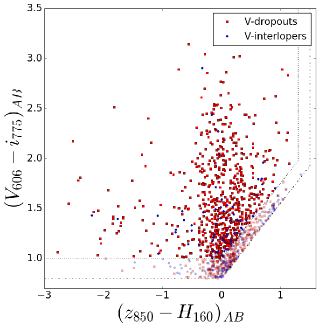
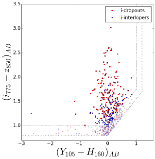
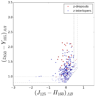
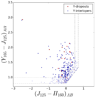
Figure 1.— Color-color selection box used to identify $V_{\rm 606}\,$- (upper left), $i_{\rm 775}\,$- (upper right), $z_{\rm 850}\,$- (bottom left) and $Y_{\rm 105}\,$-dropouts (bottom right) over the GSd field. Red squares represent dropouts, i.e high-$z$ sources with no flux blueward of the Lyman-break; blue circles represent interlopers, i.e. high-$z$ candidates showing a detection in the blue bands. Dashed lines represent the boundaries of the original sample selection; dash-dotted lines represent the boundaries of the enlarged sample (see text for details). Darker symbols refer to the original selection, lighter ones to the enlarged selection.

Note that the separation between dropouts and contaminants for sources with a low $\chi^{2}_{opt}$ is arbitrary to a certain extent; for example, Bouwens et al. (2015) impose a cut at S/N$<2$, while the Brightest of Reionizing Galaxies survey (BoRG, Trenti et al. 2011) resorts to a more conservative threshold of S/N$<1.5$ in the bluest bands. Obviously, more conservative cuts entail the exclusion of a higher number of real high$-z$ sources from the selections, thus different investigators may decide to prioritize differently sample purity versus selection completeness.

3. Results

Table 2Statistics of dropouts and interlopers

	GSd				GNw				XDF				HUDF09-2
population	original sample		enlarged sample		original sample		enlarged sample		original sample		enlarged sample		original sample		enlarged sample
	number	$\%$	number	$\%$	number	$\%$	number	$\%$	number	$\%$	number	$\%$	number	$\%$	number	$\%$
$V_{\rm 606}\,$-dropouts	648	90$\pm$2	882	81$\pm$2	392	87$\pm$2	510	73$\pm$2	132	93$\pm$3	165	85$\pm$4	102	94$\pm$4	127	88$\pm$4
$V_{\rm 606}\,$-interlopers	72	10$\pm$2	205	19$\pm$2	58	13$\pm$2	189	27$\pm$2	10	7$\pm$3	28	15$\pm$4	6	6$\pm$4	17	12$\pm$4
$i_{\rm 775}\,$-dropouts	172	62$\pm$4	239	52$\pm$3	72	65$\pm$7	105	47$\pm$4	69	77$\pm$7	78	68$\pm$6	28	60$\pm$10	37	51$\pm$8
$i_{\rm 775}\,$-interlopers	106	38$\pm$4	223	48$\pm$3	39	35$\pm$7	118	53$\pm$4	20	23$\pm$7	37	32$\pm$6	16	40$\pm$10	35	49$\pm$8
$z_{\rm 850}\,$-dropouts	33	17$\pm$4	42	11$\pm$2	29	26$\pm$6	35	16$\pm$4	31	40$\pm$8	36	30$\pm$6	17	30$\pm$10	22	23$\pm$6
$z_{\rm 850}\,$-interlopers	157	83$\pm$4	322	89$\pm$2	82	74$\pm$6	180	84$\pm$4	47	60$\pm$8	85	70$\pm$6	37	70$\pm$10	73	76$\pm$6
$Y_{\rm 105}\,$-dropouts	17	10$\pm$3	27	8$\pm$2	54	36$\pm$6	62	26$\pm$4	6	50$\pm$20	10	40$\pm$20	12	21$\pm$8	15	17$\pm$6
$Y_{\rm 105}\,$-interlopers	150	90$\pm$3	329	92$\pm$2	96	64$\pm$6	177	74$\pm$4	6	50$\pm$20	15	60$\pm$20	45	79$\pm$8	71	83$\pm$6

In this section we present and discuss our results obtained separately for the four field we analyze (GSd, GNW, XDF, HUDF09-2). However, we only show plots for GSd, to avoid unnecessary repetitions.

3.1. Numbers and redshift distribution of dropouts and interlopers

The color-color selection of dropouts and interlopers is shown in Figure 1 for samples of $V_{\rm 606}\,$, $i_{\rm 775}\,$, $z_{\rm 850}\,$, and $Y_{\rm 105}\,$-dropout sources drawn from the GSd field, with discrimination between the two classes based on the S/N and optical $\chi^{2}$ (Equation 6). We note that photometric scatter is likely to play a significant role in the selection of faint objects. Indeed, more than half of the 1$\sigma$ error bars for the interlopers intersect at least one boundary of the color-color selection box. Therefore, to carry out a more comprehensive analysis, we enlarge the color-color selection box by 0.2 mag, to check for both candidate high-$z$ LBGs and interlopers that slightly fail to meet the adopted selection criteria (see also Su et al. 2011 for an alternative approach based on assigning a probability that a source belongs to the color-color selection). In the following, we will call original selection the one given in §2 (dotted line in Fig. 1), and enlarged selection the one introduced in this section (dash-dotted line in Fig. 1).

The most striking feature of Figure 1 is the relative weight of interlopers vs. dropouts, which is quantified in Table 2 for all the fields considered. We first focus on the GSd field. At lower redshift ($z\sim 5$), dropouts dominate the sample within the original selection, while the opposite situation is present at higher redshift ($z\sim 8$), when the interloper fraction is much higher. We stress that this percentage is not giving a level of contamination in our dropout sample, since the presence of sufficiently deep data at bluer wavelengths allows us to identify the interlopers. Interestingly, the situation remains qualitatively similar with our enlarged selection, although as expected the enlarged samples contain a larger fraction of interlopers. If we adopted a more conservative S/N in the sample selection (S/N$<$1.5), percentages of dropouts would be systematically smaller, but comparable within 2$\sigma$ uncertainty.

The observed behaviour is mainly due to the fact that the population of dropouts steady decreases in number for the higher redshift selections. This is primarily determined by the evolution of the luminosity function, which decreases significantly from $z\sim 5$ to $z\sim 8$ at all luminosities. In contrast, the number of interlopers in the sky remains approximately constant over a wide range of dropout selection windows. Second order effects in the evolution of the interloper population with the redshift of the Lyman break selection are complex to model, and include intrinsic evolution of their luminosity functions, change in the distance modulus and in the comoving volume of the selection, with partial offsets among them (e.g., the decrease in sensitivity because of an increase in the distance modulus is offset by an increase of the comoving volume).

Similar findings are obtained when we analyze the other fields, even though the results from the different fields highlight the presence of sample (or “cosmic”) variance, naturally expected because of galaxy clustering (see, e.g., Trenti & Stiavelli 2008). In addition, fields such as the XDF and HUDF09-2 have small areas, resulting in significant Poisson uncertainty. Finally, the difference in relative depths reached by the different surveys plays a role, which we discuss further in Section 3.4.1.

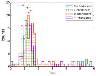
Figure 2.— Redshift distribution for the interlopers at the different dropout selections, as indicated in the labels, for the original sample over the GSd field. Photometric redshifts are drawn from the 3D-HST survey (Skelton et al., 2014). Median values along with their associated uncertainty (defined as 1.235$\times\sigma/\sqrt{n}$, with $n$ number of objects) are shown above the histograms as horizontal points with error bars.

To further investigate the properties of the interlopers, and test whether these are indeed 4000 Å break sources, we resort to the photometric redshift catalogs from the 3D-HST survey (Skelton et al., 2014), which we matched to our sources based on coordinates and $H_{\rm 160}\,$band magnitudes. The expectation is that given $z_{dropouts}$ as the redshift of the Lyman-break selection, the interlopers should be peaked at $z_{interlopers}$ given by:

$$1+z_{interlopers}=\frac{1216}{4000}\times(z_{dropouts}+1).$$ (7)

So, for example, for z = 5 selection, the interlopers are predicted to be found at $z\sim 0.7-1.0$ corresponding to the Balmer and 4000Å breaks; for z=8 selection, the interlopers are expected at $z\sim 1.6-1.9$. Taking into account uncertainties, this is broadly the case based on the photo-$z$ analysis, as shown in Figure 2 for the GSd field. For this field, after the match with the 3D-HST survey, we recover $\sim 85\%$ of our sources. From this figure, and from Equation 7, it is clear that as $z_{dropouts}$ increases, $\langle z_{interlopers}\rangle$ changes relatively little ($\Delta(z)<1$). The error on the median values narrows as we go from lower to higher redshift, but this is mainly due to the larger sample statistics provided by the $Y_{\rm 105}\,$-interlopers with respect to the $V_{\rm 606}\,$-interlopers. The fact that not all interlopers of a given selection fall exactly in the expected redshift window, and the lower than expected median redshift of the Y-interlopers highlight the limitations of both our selection method and photo-z techniques. Indeed, some real dropouts might be misclassified due to photometric scatter and/or the photo-z estimates might not be reliable. Similar trends are obtained also for the other fields, even though uncertainties are very large.

Thus, extrapolating the trend to even higher redshift samples of dropouts, such as those accessible by JWST observations, one expects that the number of interlopers in the color-color selection will remain relatively constant, while dropout numbers will decrease very rapidly for $z_{dropouts}>10$ based on theoretical modeling (see, e.g., Mason et al. 2015).

We note that, according to the Madau-Lilly plot (e.g. Madau & Dickinson 2014), the star formation rate peaks at intermediate redshift ($z\sim 2$). This means that the number density of interlopers for $z_{interlopers}\gtrsim 1.85$ (corresponding to $z_{dropouts}\sim 9.5$ from Equation 7) may likely slightly decrease with increasing redshift, although the decrease of the interloper density will still be less steep than the one of the dropouts because the latter have significantly higher redshift.

3.2. Surface densities of dropouts and interlopers

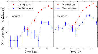
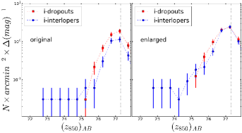
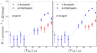
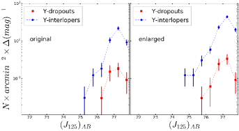
Figure 3.— Surface density distribution of dropouts (red) and interlopers (blue) in the original (left) and enlarged (right) samples for the selections at the different redshifts, as indicated in the labels, for the GSd field. The black vertical line indicates the formal 5$\sigma$ magnitude limit (Bouwens et al., 2015).

In the previous section we have investigated the incidence of dropouts and interlopers at the different redshifts. We now aim at characterizing the distribution of luminosity for these populations, to study how they compare. Thus, we derive the surface density distributions of dropouts and interlopers by counting the number of objects in each bin of 0.5 magnitudes and dividing it by the area of the survey, as shown in Figure 3 for the GSd field. For each population, the surface density is plotted as a function of $i_{\rm 775}\,$for the $z\sim 5$ samples, $z_{\rm 850}\,$for the $z\sim 6$ samples, $Y_{\rm 105}\,$for the $z\sim 7$ samples and $J_{\rm 125}\,$for the $z\sim 8$ samples. These are the magnitudes in the band that best matches the 1600 Å rest-frame at that redshift for the dropouts, as done in Bouwens et al. (2015). We note that for $m_{AB}\gtrsim 27$ (see the exact value for each magnitude as dotted line in Fig. 3) all our samples suffer from incompleteness, which is the cause of the apparent decline in the number counts of faint objects.

Surface density distributions strongly depend on the redshift and on the population considered. At the lowest redshift, the surface density distribution of interlopers is relatively flat with magnitude for $20\leq$ $i_{\rm 775}\,$$\leq 28$ and there are about 0.1 interlopers per $arcmin^{2}$ in bins of magnitude. In contrast, the distribution of dropouts rises very steeply. As expected due to the well established exponential cut off of the luminosity function at the bright end (e.g. Bouwens et al., 2015; Bowler et al., 2014; Oesch et al., 2014; McLure et al., 2013; Schenker et al., 2013), there are essentially no dropouts brighter than $i_{\rm 775}\,$$\sim$24. Overall, dropouts are much more numerous than interlopers. Similar conclusions are reached in both the original and enlarged samples.

Moving to higher redshift, the shape of the distribution of dropouts stays almost constant, just showing a modest steepening, but that of interlopers considerably changes. At $z\sim 6$, interlopers and dropouts have similar distributions, with the exception that interlopers extend toward brighter magnitudes. At $z\sim 7$ and $z\sim 8$ interlopers are more numerous than dropouts at all luminosities, and have a tail of objects at the bright-end as well. Overall, the interloper distribution appears as steep as the dropout one. This holds both for the original and the enlarged samples. Similar results are found also in the other fields.

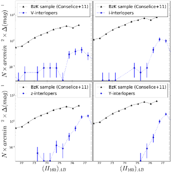
Figure 4.— $H_{160}$ surface density distribution of interlopers (blue) in the original sample for the selections at the different redshifts, as indicated in the labels, for the GSd field. Samples of BzK selected samples, drawn from (Conselice et al., 2011), are shown from comparison. The black vertical line indicates the formal 5$\sigma$ magnitude limit (Bouwens et al., 2015).

It is reasonable to expect that interlopers are a subpopulation of BzK color- selected galaxies (Daddi et al., 2004, 2007). This method is designed to find red, dusty or passively evolving older galaxies at $z>1.5$. We can therefore compare our derived surface densities of interlopers to those of BzK selected samples. We use as reference the dataset presented by Conselice et al. (2011) for galaxies at $1.5<z<3$ drawn from GOODS North and South fields and the GOODS NICMOS Survey. That study analyses two of the same fields considered in our work and includes HST imaging, therefore reaching a deeper magnitude limit compared to the many studies of BzK samples conducted from the ground (e.g. Cirasuolo et al. 2007, Hartley et al. 2008). Conselice et al. (2011) quote the $H_{\rm 160}\,$-magnitude distribution of all galaxies at $1.5<z<3$, without splitting them into redshift bins, so a direct comparison to our results is not possible because our interloper samples are more localized in redshift (see Fig.2). Still, to have a first-order approximation, we treat the Conselice et al. (2011) sample as uniform in redshift, and thus we simply rescale the observed number counts to take into consideration the difference in volume with our selections.

Figure 4 compares the Conselice et al. (2011) scaled distribution to the $H_{\rm 160}\,$-band number counts for our interlopers samples in the GSd field. At each magnitude and in each redshift bin, the BzK population is up to a factor of 10 larger than that of interlopers. This is consistent with the assumption that not all galaxies at $z\sim 1.5-2$ are interlopers of high redshift selections, but only the subset with a particular combination of colors. Interestingly, we observe that the interloper counts get steeper at faint luminosities with increasing redshift compared to the general BzK sample. This might suggest that interlopers evolve differently compared to the general population, but investigating this trend in more details is beyond the scope of this work.

3.3. Distribution of optical $\chi^{2}$ for interlopers

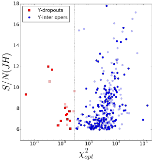
Figure 5.— Comparison between the ${\rm S/N(JH_{\rm{det}})}$ and the optical $\chi^{2}$ for $Y_{\rm 105}\,$-dropouts for the GSd field. Colors and symbols are as in Fig. 1. The dotted vertical line indicates the separation between interlopers and dropouts adopted in this work.

One of the aims of our analysis is to derive an estimate of the contamination in dropout samples. Before proceeding, we need to characterize the distribution of the optical $\chi^{2}$ values for interlopers as a function of their S/N in the detection bands. It is evident that the robustness of the detection is a key quantity to distinguish between interlopers and dropouts. In fact, while less deep observations in the redder bands give smaller ${\rm S/N(JH_{\rm{det}})}$ and simply exclude galaxies both from the dropout and interloper populations, less deep observations in the bluer bands produce lower $\chi^{2}_{opt}$ and may induce a mis-classification, moving sources from the interloper to the dropout population.

Figure 5 plots the ${\rm S/N(JH_{\rm{det}})}$ to the $\chi^{2}_{opt}$ for both dropouts and interlopers from the $z\sim 8$ selection ($Y_{\rm 105}\,$Lyman-break selection), for the GSd field. As expected, the interlopers have a positive correlation between the two quantities, reflecting the finite amplitude of the 4000 Å break. Similar results also hold for samples from selections at lower $z$ and drawn from the other fields.

3.4. Contamination in dropout samples

Now that we characterized the properties of interlopers, we can use them to investigate dropout sample contamination induced by interlopers that are mis-classified as dropouts in absence of sufficiently deep data at bluer wavelengths. The main causes of contamination are the impact of noise in the measurement of the optical $\chi^{2}$ and photometric scatter in the color-color selection.

Table 3Statistics of dropouts and interlopers after the MCMC experiment that introduces spurious noise on the observations

	GSd		GNw		XDF		HUDF09-2
population	original sample	enlarged sample	original sample	enlarged sample	original sample	enlarged sample	original sample	enlarged sample
	$\%$	$\%$	$\%$	$\%$	$\%$	$\%$	$\%$	$\%$
$V_{\rm 606}\,$-dropouts	72$\pm$2	69$\pm$2	71$\pm$3	66$\pm$3	75$\pm$6	72$\pm$5	81$\pm$6	78$\pm$6
$V_{\rm 606}\,$-interlopers	28$\pm$2	31$\pm$2	29$\pm$3	34$\pm$3	25$\pm$6	28$\pm$5	19$\pm$6	22$\pm$6
$i_{\rm 775}\,$-dropouts	32$\pm$3	30$\pm$3	34$\pm$6	30$\pm$4	52$\pm$8	47$\pm$7	33$\pm$9	29$\pm$7
$i_{\rm 775}\,$-interlopers	68$\pm$3	70$\pm$3	66$\pm$6	60$\pm$4	48$\pm$8	53$\pm$7	67$\pm$9	71$\pm$7
$z_{\rm 850}\,$-dropouts	48$\pm$2	4$\pm$1	9$\pm$3	7$\pm$2	9$\pm$5	8$\pm$4	8$\pm$5	7$\pm$4
$z_{\rm 850}\,$-interlopers	52$\pm$2	96$\pm$1	91$\pm$3	93$\pm$2	91$\pm$5	92$\pm$4	92$\pm$5	93$\pm$4
$Y_{\rm 105}\,$-dropouts	2$\pm$1	2.2$\pm$0.1	4$\pm$2	3$\pm$1	4$\pm$7	5$\pm$5	5$\pm$4	4$\pm$3
$Y_{\rm 105}\,$-interlopers	98$\pm$1	97.8$\pm$0.1	96$\pm$2	97$\pm$1	96$\pm$7	95$\pm$5	95$\pm$4	96$\pm$3

To estimate the impact of noise in the measurements on the datasets we analyzed, we perform a resampling Monte Carlo (MC) simulation on the entire photometric catalogs and add zero-mean noise in the fluxes sampling from a Gaussian distribution with width determined by the S/N ratio of the simulated broadband fluxes. We then apply the dropout selection criteria given in Sec.2, and quantify the number of interlopers and dropouts in the simulated sample. We repeat the procedure 500 times to collect statistics and we find that on average increasing the noise we obtain systematically larger fractions of interlopers at any redshift than those obtained with the original catalogs (Tab.2). The average statistics are given in Tab.3 for each field separately. This test emphasizes the need of precise photometry to robustly distinguish between dropouts and interlopers.

We note that if instead of using the entire catalogs as starting point of the MC experiment we used only a combination of the dropout and interloper enlarged samples, we would get results in agreement within the errors, indicating that actually only the sources close to the boundaries of our selection boxes can contaminate the samples.

As the next step, we also consider the photometric scatter and perform a more sophisticated resampling MC simulation on the photometric catalogs. Specifically, for each dropout selection, we uniformly sample with repetition the luminosity in the detection band from the catalog of enlarged interlopers, extracting a simulated catalog with the same size as the original one. Next, we assign to each of these objects the broadband colors of a random galaxy from the same catalog (again using uniform sampling probability with repetition), and we add zero-mean noise in the fluxes sampling from a Gaussian distribution with width determined by the S/N ratio of the simulated broadband fluxes. We use as our starting point a catalog that includes all the $Y_{\rm 105}\,$-interlopers detected in our four fields (enlarged samples), in order to consider a population that is relatively homogenous, but statistically significant. Note that for this second test it would not be appropriate to resort to the photometric catalogs of all sources, since the MC procedure effectively “re-shuffles” colors of galaxies, thus a relatively uniform starting sample is needed. Finally, we perform the photometric analysis of the catalog to quantify the number of interlopers in the enlarged sample that are classified as dropouts. After repeating the procedure 500 times to collect statistics, for example for the GSd field we find that on average:

• The $z\sim 5$ selection has 17$\pm$4 interlopers entering the $V_{\rm 606}\,$-dropout sample as contaminants, for an estimated contamination rate $f_{c}\sim 17/648\sim 2.6\%$;

• The $z\sim 6$ selection has 7$\pm$2 interlopers entering the $i_{\rm 775}\,$-dropout sample as contaminants, for an estimated contamination rate $f_{c}\sim 7/172\sim 4.0\%$;

• The $z\sim 7$ selection has 2$\pm$1 interlopers entering the $z_{\rm 850}\,$-dropout sample as contaminants, for an estimated contamination rate $f_{c}\sim 2/33\sim 6.0\%$;

• The $z\sim 8$ selection has 1$\pm$1 interlopers entering the $Y_{\rm 105}\,$-dropout sample as contaminants, for an estimated contamination rate $f_{c}\sim 1/17\sim 5.9\%$.

Overall, results from the different fields are in agreement, indicating that the contamination is always only a few percent in all samples, and it increases with increasing redshift. These results are also in broad agreement with other literature estimates, as it will be discussed in Sec.4.

These results are clearly illustrating that while the number of mis-classified interlopers remains relatively constant across different samples, as the redshift increases, the relative weight compared to the number of dropouts grows significantly. Interestingly, these estimates are consistent with the predictions from the contamination model based on source simulations from an extensive SED library encompassing a wide range of star formation histories, metallicities, and dust content and a combination of an old and a young population (Oesch et al., 2007), and used for the BoRG survey sample purity analysis (e.g., see Trenti et al. 2011; Bradley et al. 2012; Calvi et al. 2016). Applying the color cuts adopted in the current work, the model predicts a contamination of 0.7% at $z\sim 5$, 1.6% at $z\sim 6$, 3.5% at $z\sim 7$ and 7.3% at $z\sim 8$.

3.4.1 Contamination at $z\sim 8$

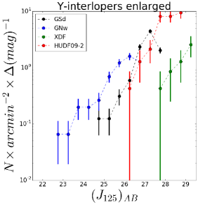
Figure 6.— Surface density distribution of $Y_{\rm 105}\,$-interlopers in the enlarged samples for all the fields considered in this study, as indicated in the labels. Each sample is plotted down to its formal 5$\sigma$ magnitude limit (from Bouwens et al., 2015). The best power law fit of the sample is $\log(N/arcmin^{2}/\Delta(mag))=(0.35\pm 0.1)\times$ $J_{\rm 125}\,$$+(-9.0\pm 0.4)$.

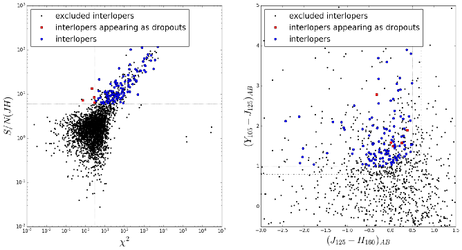
Figure 7.— Results of one realization of our MonteCarlo extraction aimed at testing the reliability of the interloper-dropout selection in deeper surveys ($J_{\rm 125}\,$$\leq$30) for a XDF-like survey (see text for details). Left: comparison between the ${\rm S/N(JH_{\rm{det}})}$ and the optical $\chi^{2}$. Dotted lines represent the detection thresholds. Right: color-color selection box used to identify $Y_{\rm 105}\,$-dropouts. Blue squares represent interlopers, red squares dropouts and black dots galaxies that do not enter anymore the selection after the dimming procedure. Dotted and dash-dotted lines are as in Fig. 1.

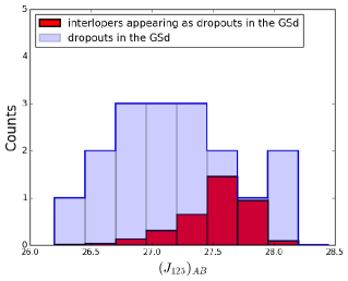
Figure 8.— $J_{\rm 125}\,$magnitude distribution for the sample of $Y_{\rm 105}\,$-dropouts in the GSd as derived from the cuts in Sec.2 (blue) and for the average contamination from dropouts as obtained from our Monte Carlo simulation (red) (see text for details).

We now focus only on the highest redshift selection ($z\sim 8$), since it contains the largest number of interlopers, and investigate more in detail the level of contamination in the different surveys.

Using a similar approach to that presented in the previous section, we can use the multi-band photometric catalog of all the interlopers identified in the different fields (enlarged sample), combined with an extrapolation of the surface number densities of interlopers, in order to estimate the contamination in different surveys, assuming that the spectral energy distributions of the interlopers are representative of the general population. We simulate a series of surveys with relative depths in the different bands similar to those used in our analysis, but different values of 5$\sigma$ depth.

For the simulation, we compute the brightness distribution of all the $Y_{\rm 105}\,$-interlopers in the enlarged sample (Fig.6). For a basic characterization of the luminosity distribution, we fit the populations using a power law through a Markov Chain Monte Carlo method. The best power law fit of the sample is $\log(N/arcmin^{2}/\Delta(mag))=(0.35\pm 0.1)\times$ $J_{\rm 125}\,$$+(-9.0\pm 0.4)$. As shown in Fig.6, while trends for the GSd and HUDF09-2 are compatible within the errors, the GNw field seems to have a systematically larger number of interlopers, while the XDF has a systematically lower number. This plots confirms that there is significant cosmic variance across fields. Quite interestingly, GNw not only has an excess of interlopers, but there is also an excess of genuine high redshift candidates reported by many studies Finkelstein et al. (2013); Oesch et al. (2014); Bouwens et al. (2015) and across a range of redshifts. Further medium/deep lines of sights beyond those available in the HST archive would be very interesting to investigate in greater detail this correlation.

We then assume that all interlopers in the sky follow a power-law fit to the number counts distribution, extrapolated in the magnitude range $J_{\rm 125}\,$=22-31, and we sample from this distribution a catalog of object luminosities. Next, we proceed to estimate the contamination in each field separately. We assign to each simulated object the broadband colors of a random galaxy from one of our interloper sample (GSd, GSw, XDF, HUDF-092), and add to the signal in each band a Gaussian noise drawn from a distribution with dispersion associated to the S/N that would be achieved in the simulated survey (following the depths reported in Tab.1). Finally, we apply the dropout selection criteria given in Sec.2, and quantify the number of simulated interlopers that satisfy the dropout selection. This gives us our best estimate of the surface number counts of contaminants in each simulated survey.

For the GSd simulation, based on the extrapolated number density of interlopers for 22$\leq$$J_{\rm 125}\,$$\leq$31 and an assumed area of $64.5$ arcmin², we extract $4390$ simulated galaxies per realization, and we repeated the simulation 500 times. On average, we find that a realization has 4$\pm$2 of these simulated interlopers appearing as dropouts, 120$\pm$10 are correctly classified as interlopers, while the remaining either turn out to have ${\rm S/N(JH_{\rm{det}})}<6$, or colors outside the selection box, and do not enter in the interloper or dropout sample. To illustrate the MC experiment, results are shown in Fig. 7 for one of the 500 realizations. This implies that the probability of mis-classifying a specific (enlarged sample) interloper as dropout is very small $p\sim 0.001$.

Figure 8 shows the $J_{\rm 125}\,$magnitude distribution for observed dropouts in the GSd, selected with the criteria given in Sec.2. Overplotted is also the average magnitude distribution of the simulated contaminants (i.e. interlopers appearing as dropouts after the MC experiment). It can be clearly seen that the fraction of contamination increases at fainter magnitudes, consistent with the explanation that photometric scatter is the main cause of contamination.

Repeating the MC experiment for the other fields, we found that for the GNw/XDF/HUDF09-2 simulation, on average, a realization has 1$\pm$1/1$\pm$1/1$\pm$1 of the simulated interlopers appearing as dropouts, and 53$\pm$7/45$\pm$6/25$\pm$5 that are correctly classified as interlopers. This implies that the probability of mis-classifying a specific (enlarged sample) interloper as dropout is very small in all the fields ($p\sim 0.0002/0.003/0.003$). The GNw field is the one with the lowest contamination. As shown in Tab.1, this field has the deepest relative depth blueward of the dropout band compared to the detection band, and clearly this allows more efficient identification of interlopers, minimizing contamination of the dropout sample. In fact, even though the other fields have deeper photometry, their photometric limits in the blue bands are relatively shallower compared to the limits of the detection (red) bands, inducing a higher probability of misclassification of interlopers as dropouts (and therefore higher contamination).

Overall, our analysis also suggests that given a survey, the higher the S/N in the detection, the higher the likelihood that the dropout is a LBG. Thus we are fully consistent with the high sample purity inferred from spectroscopic follow-up studies of LBG samples in ultradeep surveys (e.g. Malhotra et al. 2005) since spectroscopic investigations are limited to the brighter galaxies (e.g. $m\lesssim 27.5$).

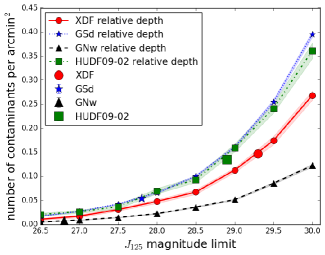
Figure 9.— Estimated level of contamination in $Y_{\rm 105}\,$-dropout surveys due to misidentified interlopers depending on survey magnitude limits. Different colors refer to different observational choices (relative depths and filter types) used a reference, as indicated in the label. Errors are the errors on the mean of the 500 realizations.

To explore how contamination changes as a function of the limiting depth of the survey, we repeat the MC experiments varying the $J_{\rm 125}\,$band magnitude limit and scaling the limits in all other bands keeping the relative depths constants The results are shown in Figure 9 which summarizes the level of contamination per arcmin² versus limiting magnitude. As expected, the contamination increases toward fainter magnitudes, because there is a higher number of potential contaminants, and strongly depends on the relative limiting depths of the different bands. Overall, the level of contamination ranges between $\sim$0 and $\sim 0.4$ contaminants per arcmin² in the magnitude range $J_{\rm 125}\,$=26.5-30. As already mentioned, the relative depth of the GNw seems to do the best job in discriminating interlopers and dropouts, therefore the contamination is the smallest.

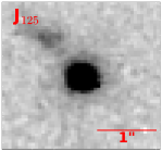
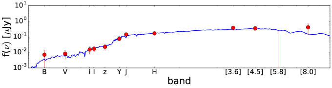
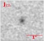
Figure 10.— Examples of SEDs and images in the band of detection for $Y_{\rm 105}\,$-interlopers that appear as dropouts at $z\sim 8$ (right) after the MC experiment. SED fitting has been obtained the photometry with FAST (Kriek et al., 2009).

Our conclusion on the presence of a significant level of contamination near the detection limit of a survey because of significant photometric scatter is indirectly supported by a cross-matching analysis of the catalogs for $i_{\rm 775}\,$and $Y_{\rm 105}\,$-dropouts in the XDF/GOODS-South published by McLure et al. (2013) and Bouwens et al. (2015), which shows that less than $50\%$ of the sources appear in both catalogs within one magnitude of the survey detection limit, even though the derived luminosity functions are similar (see Barone-Nugent et al. 2014).

3.5. Properties of the $Y_{\rm 105}\,$-contaminants

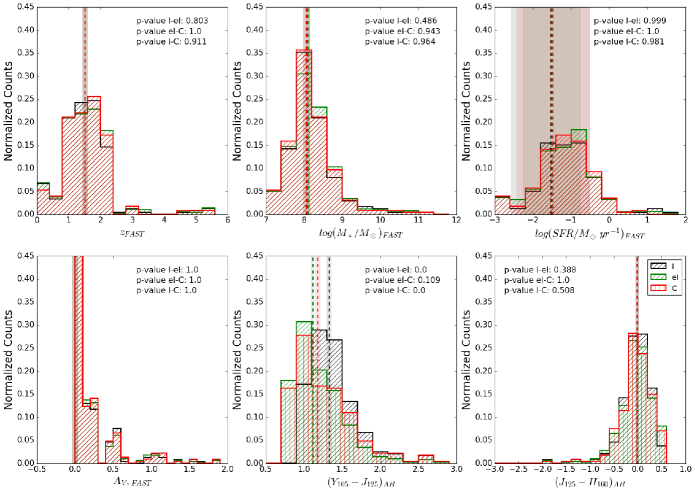
Figure 11.— Distribution of redshifts, stellar masses, star formation rates, dust extinctions and colors for Y-interlopers in the original sample (“I”, black lines), Y-interlopers in the enlarged sample (“eI”, green lines), and for interlopers appearing as contaminants after the MC experiment (“C”, red lines). Stellar population properties have been estimated from the photometry with FAST (Kriek et al., 2009). Values indicated are the probabilities that two distributions are drawn from the same parent distribution, according to the Kolmogorov-Smirnov test.

To investigate what are the properties of the objects that can migrate from the interloper to the dropout sample when their photometry is rescaled to fainter fluxes (and therefore lower S/N), we report in Figure 10 some examples of interlopers in the enlarged sample that after the MC dimming experiment appear as dropouts at $z\sim 8$. As it is clear from the SEDs, these objects are bright in the band of detection, but their 4000 Å is sufficiently deep that the faint flux at bluer wavelengths is not detected after the typical dimming of $\sim 3-4$ mag that our MC experiment assigns to simulated objects near the XDF detection limit. The figure also highlights the key assumption (and potential limitation) of our approach, that is the use of SEDs observed in brighter galaxies for modeling the colors of fainter sources.

To further characterize the interlopers and especially those that after the dimming appear as dropouts, we derive their stellar population properties by fitting the observed SEDs from the F435W to the F160W or to the Spitzer-IRAC 8$\mu m$ photometry, depending on availability, using FAST (Kriek et al., 2009). We adopt Bruzual & Charlot (2003) models assuming exponentially declining Star formation histories (SFHs) of the form $SFR\propto\exp{-t/\tau}$, where $SFR$ is the star formation rate, $t$ is the time since the onset of star formation, and $\tau$ sets the timescale of the decline in the SFR, solar metallicity, a Calzetti et al. (2000) dust law, and a Chabrier (2003) Inital Mass Function (IMF). We allow $\log(\tau/Gyr)$ to range between 7.0 and 10.0 Gyr, $\log(t/Gyr)$ between 7.0 and 10.1 Gyr, and $A_{V}$ between 0 and 4 mag. When possible, we also use photometric redshifts from the 3D-HST survey (Skelton et al., 2014), to further constrain the fits.

Overall, across the different field, 273 $Y_{\rm 105}\,$-interlopers appear as contaminants in at least one out of the 500 MC realizations. We expect this sample to be representative of the entire contaminant population.

A summary of the typical properties of the interlopers and of those that might contaminate the dropout samples at $z\sim 8$ is given in Table 4. The distributions of some properties are also presented in Fig. 11. Interestingly, both interlopers and contaminants have intermediate ages, low level of ongoing star formation and only a moderate dust content. Both medians value and Kolmogorov-Smirnov tests support the similarity of the distributions. As expected given the fact that our contaminants are drawn from the enlarged sample, which by construction includes objects up to 0.2 mag bluer than interlopers, interlopers have a noticeably redder $Y_{\rm 105}\,$-$J_{\rm 125}\,$color than contaminants. These estimates are consistent with the typical values of dust content and ages obtained from the contamination model based on source simulations from an extensive SED library used in Sec. 4.1.3. This result suggests that it is reasonable to expect that such properties can scale from the intermediate mass objects used as templates to the lower mass and fainter sources that would be contaminants in actual datasets.

Table 4Stellar population properties of all $Y_{\rm 105}\,$-interlopers and of those appearing as dropouts after the MC experiment.

property	$Y_{\rm 105}\,$-interlopers	$Y_{\rm 105}\,$-contaminants
$z$	1.51$\pm$0.07	1.51$\pm$0.07
($Y_{\rm 105}\,$-$J_{\rm 125}\,$)AB	1.33$\pm$0.03	1.21$\pm$0.04
($J_{\rm 125}\,$-$H_{\rm 160}\,$)AB	-0.03$\pm$0.04	-0.02$\pm$0.04
$\log(M_{\ast}/M_{\sun})$	8.07$\pm$0.08	8.06$\pm$0.06
$\log(SFR/(M_{\sun}\,yr^{-1})$	-1.0$\pm$1	-1.5$\pm$0.9
$\log(SSFR/yr^{-1})$	-9.5$\pm$0.9	-9.5$\pm$0.8
$A_{V}$	0.00$\pm$0.03	0.00$\pm$0.03
$\log(\tau/Gyr^{-1})$	8.0$\pm$0.1	8.0$\pm$0.1
$\log(t/Gyr^{-1})$	8.60$\pm$0.04	8.60$\pm$0.04

4. Contamination estimates in the literature

In the literature, there have been various studies that tried to give an estimate of the contamination in the dropouts sample, with the intent to correct the estimates of the luminosity functions, but not to characterize the properties of the contaminants. Each of these studies has used a different definition for the dropout/interloper sample and evaluated the contamination in a different way, so a direct comparison among the different findings is not always possible and have to be considered carefully.

Here, we present a summary of some important literature results and then we will redo our analysis using the same selection criteria adopted by Bouwens et al. (2015), with the aim of directly compare our and their findings.

Bouwens et al. (2015) have estimated the impact of a scattering into a color selection windows owing to the impact of noise by repeatedly adding noise to the imaging data from the deepest fields, creating catalogs, and then attempting to reselect sources from these fields in exactly the same manner as the real observations. Sources that were found with the same selection criteria as the real searches in the degraded data but that show detections blueward of the break in the original observations were classified as contaminants. They estimated the likely contamination by using brighter, higher-S/N sources in the XDF to model contamination in fainter sources. They estimated a contamination rate of 2$\pm$1%, 3$\pm$1%, 6$\pm$2%, 10$\pm$3%, and 8$\pm$2% at $z\sim 4$, $z\sim 5$, $z\sim 6$, $z\sim 7$, and $z\sim 8$, respectively.

These results are in agreement to ours (see also Sec.4.1.1) and to those found in other recent selections of sources in the high-redshift universe (e.g., Giavalisco et al., 2004; Bouwens et al., 2006, 2007, 2012b; Wilkins et al., 2011; Schenker et al., 2013).

Finkelstein et al. (2015) found instead larger values of contamination. They estimated the contamination by artificially dimming lower redshift sources in their catalog, to see if the increased photometric scatter allows them to be selected as high-redshift candidates. For sources with 25$<$$H_{\rm 160}\,$$<$27, they estimated a contamination fraction of 4.5%, 8.1%, 11.4%, 11.1%, and 16.0% at $z\sim 4$, $z\sim 5$, $z\sim 6$, $z\sim 7$, and $z\sim 8$, respectively. For fainter sources with 26$<$$H_{\rm 160}\,$$<$29, the contamination fraction increased to 9.1%, 11.6%, 6.2%, 14.7%, and $<$4.9% at $z\sim 4$, $z\sim 5$, $z\sim 6$, $z\sim 7$, and $z\sim 8$, respectively. These fractions are in line with the estimates from the stacked probability distribution curves (e.g. Malhotra et al., 2005).

Casey et al. (2014), by studying the space density of the potentially contaminating sources, found that dusty star-forming galaxies at $z<5$ might contaminate $z>5$ galaxy samples at a rate of $<1\%$. Such fraction might increase when photometric scatter is applied to faint, red galaxies, making it easier for them to scatter into high-z samples (Finkelstein et al., 2015).

To minimize the probability of contamination by low-redshift interlopers, the BoRG strategy was to impose a conservative non-detection threshold of 1.5$\sigma$ on the optical-band data (Bradley et al., 2012; Trenti et al., 2011). In order to estimate the residual contamination, from the Bouwens et al. (2010) data reduction they first identified F098M dropouts with F125W$<$27 considering a version of the GOODS F606W image degraded to a 5$\sigma$ limit F606W = 27.2 to match the relative F125W versus F606W BoRG depth. They then checked for contaminants by rejecting F098M dropouts with $S/N>2$ in either B, V, or i (at their full depth). They estimated approximately 30% contamination, which is much higher to what we found, but in good agreement with the estimate based on the application of the color selection to libraries of SED models (Oesch et al., 2007).

Note that the key difference between BoRG and other surveys is that BoRG only has one blue band, making the identification of contaminants more difficult.

4.1. The Bouwens et al. 2015 cuts

4.1.1 Sample selection

We now repeat our analysis adopting the cuts proposed by Bouwens et al. (2015), in order to test how a different sample selection may alter our conclusions. For the sake of brevity, we report our analysis performed only on the CANDELS/GOODS South deep imaging (Grogin et al., 2011). The parent catalog is the one presented in §2. We apply the same cut in $S/N(JH_{\rm{det}})$ and stellarity index described in §2.

We then apply the following color selection criteria for samples of LBGs in the redshift range $z\sim 5-8$, based on Bouwens et al. (2015).

For $z\sim 5$ candidates

$$\begin{split}V_{606}-i_{775}&>1.2\\ z_{850}-H_{160}&<1.3\\ V_{606}-i_{775}&>0.8(z_{850}-H_{160})+1.2\end{split}$$ (8)

For $z\sim 6$ candidates

$$\begin{split}i_{775}-z_{850}&>1.0\\ Y_{105}-H_{160}&<1.0\\ i_{775}-z_{850}&>0.78(Y_{105}-H_{160})+1.0\end{split}$$ (9)

For $z\sim 7$ candidates

$$\begin{split}z_{850}-Y_{105}&>0.7\\ J_{125}-H_{160}&<0.45\\ z_{850}-Y_{105}&>0.8(J_{125}-H_{160})+0.7\end{split}$$ (10)

For $z\sim 8$ candidates

$$\begin{split}Y_{105}-J_{125}&>0.45\\ J_{125}-H_{160}&<0.5\\ Y_{105}-J_{125}&>0.75(J_{125}-H_{160})+0.525.\end{split}$$ (11)

To distinguish between interlopers and dropouts, we use the following cuts in S/N. According to Bouwens et al. (2015), $V_{\rm 606}\,$-dropouts are selected as sources with S/N($B_{\rm 435}\,$)$<$2, $i_{\rm 775}\,$-dropouts with S/N($B_{\rm 435}\,$)$<2$ and either ($V_{\rm 606}\,$- $z_{\rm 850}\,$)$>$ 2.7 or S/N($V_{\rm 606}\,$)$<2$, $z_{\rm 850}\,$- and $Y_{\rm 105}\,$dropouts with S/N($x$)$<2$ and $\chi^{2}_{x}<3$, where $x$ is intended to be $B_{\rm 435}\,$, $V_{\rm 606}\,$, and $i_{\rm 775}\,$bands for $z_{\rm 850}\,$-dropouts and $B_{\rm 435}\,$, $V_{\rm 606}\,$, $i_{\rm 775}\,$and $I_{\rm 814}\,$ bands for $Y_{\rm 105}\,$-dropouts (Eq.6). In addition, $z_{\rm 850}\,$-dropouts are also selected as sources with either ($I_{\rm 814}\,$-$J_{\rm 125}\,$$)>$1.0 or S/N($I_{\rm 814}\,$)$<$1.5.

As before, if a dropout satisfies more than one dropout selection, we assign it to the highest redshift sample. This additional cut removes $\sim 30$ sources from the $z_{\rm 850}\,$- selection, while in the other cases at most a few sources are removed. In contrast, we do not apply this restriction to interlopers, which thus may enter multiple selections. However, only very few galaxies enter simultaneously more than one selection, therefore results are not driven by this subpopulation of duplicates.

4.1.2 Results

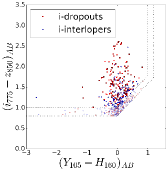
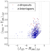
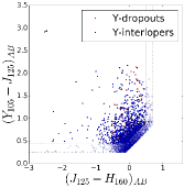
Figure 12.— Color-color selection box used to identify $V_{\rm 606}\,$- (upper left), $i_{\rm 775}\,$- (upper right), $z_{\rm 850}\,$- (bottom left) and $Y_{\rm 105}\,$-dropouts (bottom right), following the color selection presented in Bouwens et al. (2015). Red squares represent dropouts, i.e high-$z$ sources with no flux blueward of the Lyman-break; blue circles represent interlopers, i.e. high-$z$ candidates showing a detection in the blue bands. Dashed lines represent the boundaries of the original sample selection, following Bouwens et al. (2015); dash-dotted lines represent the boundaries of the enlarged sample (see text for details). Darker symbols refer to the original selection, lighter ones to the enlarged selection.

The color-color selection of dropouts and interlopers adopting the Bouwens et al. (2015) selection is shown in Figure 12 for samples of $V_{\rm 606}\,$, $i_{\rm 775}\,$, $z_{\rm 850}\,$, and $Y_{\rm 105}\,$-dropout and interloper sources. As done in §3.1, we define an original and an enlarged selection, by simply enlarging the color-color selection box by 0.2 mag, to check for both candidate high-$z$ LBGs and interlopers that slightly fail to meet the usual selection criteria.

Table 5Statistics of dropouts and interlopers

population	original sample		enlarged sample
	number	$\%$	number	$\%$
$V_{\rm 606}\,$-dropouts	446	93$\pm$2	601	90$\pm$2
$V_{\rm 606}\,$-interlopers	33	7$\pm$2	69	10$\pm$2
$i_{\rm 775}\,$-dropouts	167	62$\pm$4	225	53$\pm$4
$i_{\rm 775}\,$-interlopers	102	48$\pm$4	215	47$\pm$4
$z_{\rm 850}\,$-dropouts	53	11$\pm$2	74	7$\pm$1
$z_{\rm 850}\,$-interlopers	443	89$\pm$2	999	93$\pm$1
$Y_{\rm 105}\,$-dropouts	45	4.1$\pm$0.9	61	2.5$\pm$0.5
$Y_{\rm 105}\,$-interlopers	1054	95.9$\pm$0.9	2418	97.5$\pm$0.5

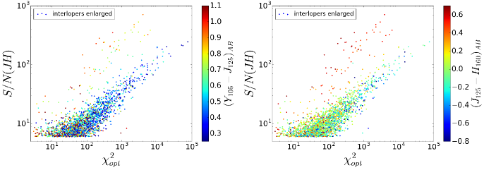
Figure 13.— Comparison between the ${\rm S/N(JH_{\rm{det}})}$ and the optical $\chi^{2}$ for interlopers in the enlarged sample at $z\sim 8$. In the right panel, the $Y_{\rm 105}\,$-$J_{\rm 125}\,$color is color-coded, while in the left panel the $J_{\rm 125}\,$-$H_{\rm 160}\,$color is color coded.

Given the fact that the Bouwens et al. (2015) criteria on the Lyman-Break color are less strict than those presented in §1, many more galaxies enter both the dropout and the interloper samples, at any redshift. Table 5 presents a summary of the incidence of each population. Comparing the fractions to those presented for the same field in Table 2, we find that the fraction of $V_{\rm 606}\,$-dropouts is the same (the changes to the selection are really minor), while at higher redshifts dropouts fraction are considerably smaller. This indicates that a more strict selection criteria does reduce the number of interlopers, even though it simultaneously reduces the sample of dropouts. Therefore each selection should be a good compromise between purity and completeness.

Similarly to what we did in the previous section, we derive the surface density distributions of dropouts and interlopers in our Bouwens et al. (2015) like selection. Results are qualitatively similar to those found for a constant color cut, with the shape of the distribution of dropouts staying almost constant with increasing redshift, while that of interlopers considerably steepening.

Inspecting a ${\rm S/N(JH_{\rm{det}})}$ vs. $\chi^{2}_{opt}$ diagram for the Bouwens et al. (2015) sample selection, it emerges that the enlarged sample appears to have objects distributed along two different sequences. To further explore this population, in Fig. 13 we focus on interlopers only and add the information on their near-IR colors. It appears evident that most of the objects in the second sequence are characterized by intermediate colors in $Y_{\rm 105}\,$-$J_{\rm 125}\,$and red colors in $J_{\rm 125}\,$-$H_{\rm 160}\,$(0.5$<$$J_{\rm 125}\,$-$H_{\rm 160}\,$$<$0.7). This demonstrates the utility of excluding candidates that are too red (e.g. Giavalisco et al., 2004; Bouwens et al., 2007, 2015). Similar results also hold for samples from selections at lower $z$.

4.1.3 Contamination in dropout samples

Mimicking the analysis in the previous section, we investigate the level of contamination in the Bouwens et al. (2015) dropout sample induced by interlopers that are mis-classified as dropouts in absence of sufficiently deep data at bluer wavelengths.

First we estimate the impact of noise in the measurement of the optical $\chi^{2}$ and photometric scatter in the color-color selection performing a resampling MC simulation on the photometric catalogs. As before, for each dropout selection, we uniformly sample with repetition the luminosity in the detection band from the catalog of enlarged interlopers, extracting a simulated catalog with the same size as the original one. Next, we assign to each of these objects the broadband colors of a random galaxy from the original parent catalog (again using uniform sampling probability with repetition), and we add zero-mean noise in the fluxes sampling from a Gaussian distribution with width determined by the S/N ratio of the simulated broadband fluxes. Finally, we perform the photometric analysis of the catalog to quantify the number of interlopers in the enlarged sample that are classified as dropouts. After repeating the procedure 500 times to collect statistics, we find that on average:

• The $z\sim 5$ selection has 7$\pm$1 interlopers entering the $V_{\rm 606}\,$-dropout sample as contaminant, for an estimated contamination rate $f_{c}\sim 7/446\sim 1.5\%$;

• The $z\sim 6$ selection has 4$\pm$1 interlopers entering the $i_{\rm 775}\,$-dropout sample as contaminant, for an estimated contamination rate $f_{c}\sim 4/167\sim 2.5\%$;

• The $z\sim 7$ selection has 5$\pm$1 interlopers entering the $z_{\rm 850}\,$-dropout sample as contaminant, for an estimated contamination rate $f_{c}\sim 5/53\sim 9.4\%$;

• The $z\sim 8$ selection has 7$\pm$1 interlopers entering the $Y_{\rm 105}\,$-dropout sample as contaminant, for an estimated contamination rate $f_{c}\sim 7/45\sim 15.3\%$.

These results are clearly illustrating that while the number of mis-classified interlopers remains relatively constant across different samples, as the redshift increases, the relative weight compared to the number of dropouts grows significantly. These estimates are systematically larger than those presented in the previous section, indicating how in the selection cuts proposed Bouwens et al. (2015) many more interlopers might be incorrectly classified as dropouts. Nonetheless, as the sample presented in the previous section, these estimates are consistent with the predictions from the contamination model based on source simulations from an extensive SED library (Oesch et al., 2007). The model predicts a contamination of 3.1% at $z\sim 5$, 0.5% at $z\sim 6$, 6.3% at $z\sim 7$ and 12.4% at $z\sim 8$. It forecasts a higher contamination at $z\sim 5$ compared to $z\sim 6$ that our MC experiment does not capture. This is likely due to the fact that, being based on the observed data, the MC at $z\sim 5$ is able to identify contaminants only when the objects show a detection in the single band ($B_{\rm 435}\,$) blueward of the break, unlike the model based on a template library.

Therefore, it appears evident that the choice of the color cuts noticeably alters the fraction of dropouts and interlopers and the estimates of contamination. The Bouwens et al. (2015) selection criteria ensure a larger number of dropouts at all redshifts, but unavoidably also a larger number of interlopers. As a consequence also the estimated contamination is considerably higher.

5. Summary and Conclusions

In this paper we investigated the contamination of photometrically selected samples of high redshift galaxies. Our focus has been on the widely adopted Lyman-break technique, using high quality multi-band imaging from the Hubble CANDELS surveys (GOODS Deep South and GOODS Wide North), the XDF and the HUDF09-2. In our analysis we distinguished between dropouts, that is sources that formally satisfy all the selection criteria of LBGs, and interlopers, that is sources with similar colors redwards of the spectral break, but showing a detection at bluer wavelengths. Because of finite photometric precision, when no sufficiently deep data at bluer wavelengths are available, a (small) fraction of interlopers can be mis-classified as dropouts, and contaminate the selection. Hence we indicated these objects as contaminants.

The class of interlopers/contaminants that we studied is that of intermediate redshift galaxies with a prominent 4000 Å/Balmer break, which are the most common among interlopers based on redshift estimates from the 3DHST survey (see Figure 2).

Our key results are the following:

• Adopting a constant cut on the strength of the Lyman break across different redshifts, the number counts of interlopers shows an increase in number with $z$ of at most a factor of 2. In contrast, in selections where the cut on the strength of the Lyman break varies with redshift (e.g. Bouwens et al., 2015), the number counts of interlopers increase significantly from $z\sim 5$ to $z\sim 8$. This suggests that cleaner samples of dropouts can be achieved by requesting a clear spectral break, which reduces the number of interlopers more significantly than the number of dropouts.

• The surface density of interlopers in the sky remains approximately constant over the range of dropout selection windows considered in this study (that is dropouts from $z\sim 5$ to $z\sim 8$), for a given depth of the survey and for a uniform cut in the color containing the Lyman break. This is because the population of interlopers resides at lower redshift and its average redshift evolves more slowly (by a factor $\sim 0.3$) compared to that of the dropouts (see Equation 7 and Figure 2). Thus, since the number of dropouts evolves rapidly with redshift, the ratio of interlopers to dropouts grows significantly with increasing redshift.

• While the shape of the surface density distribution of dropouts stays relatively constant with increasing redshift, that of interlopers possibly gets steeper. Interlopers also tend to have a tail at the bright end.

• Using a Monte Carlo resampling of the interloper population we estimate a contamination of the dropout samples in all the fields, ranging from $\sim 2\%$ at $z\sim 5$ to $\sim 6\%$ at $z\sim 8$ for the GSd field, with a clear trend of increasing contamination for higher redshift dropout samples. In the other fields, the contamination is similar, but systematically lower. The lowest level of contamination is found for GDw, indicating that having relatively deeper blue bands compared to red bands is the most effective toop to properly separate interlopers from dropouts.

• Extrapolating with a power-law the interloper number counts distribution at the faint end to simulate ultradeep surveys, we derive that the contamination increases toward fainter magnitudes, and ranges from 0.1 to 0.4 contaminants per arcmin² at $J_{\rm 125}\,$=30, depending on the field considered. Generally we find that these contaminants are located near the detection limit of the survey.

• By means of SED modeling, we characterized the stellar population properties of the interlopers that may contaminate the dropout sample, and found objects with intermediate ages ($\sim 1$ Gyr at $z\sim 1.5-2$), very-low levels of ongoing star formation, and relatively low dust content.

Our results and contamination estimates are limited by restrictions to galaxy-like sources and to Gaussian noise. The former is not likely to be an issue for space based observations with high angular resolution, but it might affect ground-based surveys that do not have the ability to discriminate between compact galaxies and stars. The assumption of normally distributed errors is again likely to underestimate the occurrence of rare, extreme events of photometric scatter, since data are likely to have an excess of noise compared to a normal distribution in their tails (Schmidt et al., 2014). Thus, our results are to be considered lower limits for the contamination of dropout samples. Also, while we focused on Lyman-break selection, a similar analysis would be expected to hold qualitatively if we had considered photometric redshift estimates to construct the sample of dropouts and interlopers, with the added complication of leaving more degrees of freedom in defining the selection and the separation between the two samples.

Overall our key conclusion is that the dropout selection of high redshift sources leads currently to samples with high purity, but the purity degrades when the number of dropouts becomes much smaller than the number of interlopers. We demonstrated this clearly for the $Y_{\rm 105}\,$-dropout sample from space observations over deep fields. A qualitatively similar conclusion on an increase of the contamination fraction is expected to hold for ground-based surveys over large areas as well, targeting the bright-end ($m\sim 24-26$) of the galaxy luminosity function at high-$z$, since the relative number of dropouts versus interlopers is significantly suppressed. However, in this case the objects are so bright that targeted follow-ups such as spectroscopic observations, should be able to discriminate between high-$z$ sources and contaminants.

Finally, extrapolating our results to future surveys at $z>10$, we highlight the need to consider carefully the contamination of the dropout samples, since the number of objects expected at such early times will be orders of magnitude smaller than the number of interlopers with similar colors, and thus the contamination might exceed $50\%$. Fortunately, in this respect, the capability of JWST to observe efficiently at rest-frame optical wavelengths for sources at $z>10$ will greatly help in continuing to select samples of photometrically selected objects with high purity, similar to the role played currently by Spitzer IRAC imaging to validate samples of bright dropouts at $z\sim 8-10$ identified by HST (Bouwens et al., 2015).

References

- Atek et al. (2011) Atek, H., Siana, B., Scarlata, C., et al. 2011, ApJ, 743, 121
- Barone-Nugent et al. (2014) Barone-Nugent, R. L., Trenti, M., Wyithe, J. S. B., et al. 2014, ApJ, 793, 17
- Bertin & Arnouts (1996) Bertin, E., & Arnouts, S. 1996, A&AS, 117, 393
- Blakeslee et al. (2003) Blakeslee, J. P., Anderson, K. R., Meurer, G. R., Benitez, N., & Magee, D. 2003, in Astronomical Society of the Pacific Conference Series, Vol. 295, Astronomical Data Analysis Software and Systems XII, ed. H. E. Payne, R. I. Jedrzejewski, & R. N. Hook, 257
- Bouwens et al. (2006) Bouwens, R. J., Illingworth, G. D., Blakeslee, J. P., & Franx, M. 2006, ApJ, 653, 53
- Bouwens et al. (2007) Bouwens, R. J., Illingworth, G. D., Franx, M., & Ford, H. 2007, ApJ, 670, 928
- Bouwens et al. (2010) Bouwens, R. J., Illingworth, G. D., Oesch, P. A., et al. 2010, ApJ, 709, L133
- Bouwens et al. (2011a) Bouwens, R. J., Illingworth, G. D., Labbe, I., et al. 2011a, Nature, 469, 504
- Bouwens et al. (2011b) Bouwens, R. J., Illingworth, G. D., Oesch, P. A., et al. 2011b, ApJ, 737, 90
- Bouwens et al. (2012a) —. 2012a, ApJ, 752, L5
- Bouwens et al. (2012b) —. 2012b, ApJ, 754, 83
- Bouwens et al. (2015) —. 2015, ApJ, 803, 34
- Bowler et al. (2012) Bowler, R. A. A., Dunlop, J. S., McLure, R. J., et al. 2012, MNRAS, 426, 2772
- Bowler et al. (2014) —. 2014, MNRAS, 440, 2810
- Bradley et al. (2012) Bradley, L. D., Trenti, M., Oesch, P. A., et al. 2012, ApJ, 760, 108
- Bradley et al. (2014) Bradley, L. D., Zitrin, A., Coe, D., et al. 2014, ApJ, 792, 76
- Bruzual & Charlot (2003) Bruzual, G., & Charlot, S. 2003, MNRAS, 344, 1000
- Bunker et al. (2003) Bunker, A. J., Stanway, E. R., Ellis, R. S., McMahon, R. G., & McCarthy, P. J. 2003, MNRAS, 342, L47
- Calvi et al. (2016) Calvi, V., Trenti, M., Stiavelli, M., et al. 2016, ApJ, 817, 120
- Calzetti et al. (2000) Calzetti, D., Armus, L., Bohlin, R. C., et al. 2000, ApJ, 533, 682
- Casey et al. (2014) Casey, C. M., Scoville, N. Z., Sanders, D. B., et al. 2014, ApJ, 796, 95
- Castellano et al. (2012) Castellano, M., Fontana, A., Grazian, A., et al. 2012, A&A, 540, A39
- Chabrier (2003) Chabrier, G. 2003, PASP, 115, 763
- Coe et al. (2015) Coe, D., Bradley, L., & Zitrin, A. 2015, ApJ, 800, 84
- Conselice et al. (2011) Conselice, C. J., Bluck, A. F. L., Buitrago, F., et al. 2011, MNRAS, 413, 80
- Daddi et al. (2004) Daddi, E., Cimatti, A., Renzini, A., et al. 2004, ApJ, 600, L127
- Daddi et al. (2007) Daddi, E., Dickinson, M., Morrison, G., et al. 2007, ApJ, 670, 156
- Dow-Hygelund et al. (2007) Dow-Hygelund, C. C., Holden, B. P., Bouwens, R. J., et al. 2007, ApJ, 660, 47
- Finkelstein et al. (2010) Finkelstein, S. L., Papovich, C., Giavalisco, M., et al. 2010, ApJ, 719, 1250
- Finkelstein et al. (2012) Finkelstein, S. L., Papovich, C., Salmon, B., et al. 2012, ApJ, 756, 164
- Finkelstein et al. (2013) Finkelstein, S. L., Papovich, C., Dickinson, M., et al. 2013, Nature, 502, 524
- Finkelstein et al. (2015) Finkelstein, S. L., Ryan, Jr., R. E., Papovich, C., et al. 2015, ApJ, 810, 71
- Gehrels (1986) Gehrels, N. 1986, ApJ, 303, 336
- Giavalisco et al. (2004) Giavalisco, M., Ferguson, H. C., Koekemoer, A. M., et al. 2004, ApJ, 600, L93
- Grogin et al. (2011) Grogin, N. A., Kocevski, D. D., Faber, S. M., et al. 2011, ApJS, 197, 35
- Guo et al. (2013) Guo, Y., Ferguson, H. C., Giavalisco, M., et al. 2013, ApJS, 207, 24
- Hayes et al. (2012) Hayes, M., Laporte, N., Pelló, R., Schaerer, D., & Le Borgne, J.-F. 2012, MNRAS, 425, L19
- Illingworth et al. (2013) Illingworth, G. D., Magee, D., Oesch, P. A., et al. 2013, ApJS, 209, 6
- Kriek et al. (2009) Kriek, M., van Dokkum, P. G., Labbé, I., et al. 2009, ApJ, 700, 221
- Lorenzoni et al. (2013) Lorenzoni, S., Bunker, A. J., Wilkins, S. M., et al. 2013, MNRAS, 429, 150
- Madau & Dickinson (2014) Madau, P., & Dickinson, M. 2014, eprint arXiv, 1403, 7
- Magee et al. (2011) Magee, D. K., Bouwens, R. J., & Illingworth, G. D. 2011, in Astronomical Society of the Pacific Conference Series, Vol. 442, Astronomical Data Analysis Software and Systems XX, ed. I. N. Evans, A. Accomazzi, D. J. Mink, & A. H. Rots, 395
- Malhotra et al. (2005) Malhotra, S., Rhoads, J. E., Pirzkal, N., et al. 2005, ApJ, 626, 666
- Mason et al. (2015) Mason, C. A., Trenti, M., & Treu, T. 2015, ApJ, 813, 21
- McLeod et al. (2016) McLeod, D. J., McLure, R. J., & Dunlop, J. S. 2016, MNRAS, 459, 3812
- McLure et al. (2010) McLure, R. J., Dunlop, J. S., Cirasuolo, M., et al. 2010, MNRAS, 403, 960
- McLure et al. (2013) McLure, R. J., Dunlop, J. S., Bowler, R. A. A., et al. 2013, MNRAS, 432, 2696
- Oesch et al. (2007) Oesch, P. A., Stiavelli, M., Carollo, C. M., et al. 2007, ApJ, 671, 1212
- Oesch et al. (2012) Oesch, P. A., Bouwens, R. J., Illingworth, G. D., et al. 2012, ApJ, 745, 110
- Oesch et al. (2014) —. 2014, ApJ, 786, 108
- Oesch et al. (2016) Oesch, P. A., Brammer, G., van Dokkum, P. G., et al. 2016, ApJ, 819, 129
- Oke & Gunn (1983) Oke, J. B., & Gunn, J. E. 1983, ApJ, 266, 713
- Ouchi et al. (2009) Ouchi, M., Mobasher, B., Shimasaku, K., et al. 2009, ApJ, 706, 1136
- Pirzkal et al. (2013) Pirzkal, N., Rothberg, B., Ryan, R., et al. 2013, ApJ, 775, 11
- Popesso et al. (2009) Popesso, P., Dickinson, M., Nonino, M., et al. 2009, A&A, 494, 443
- Schenker et al. (2013) Schenker, M. A., Robertson, B. E., Ellis, R. S., et al. 2013, ApJ, 768, 196
- Schmidt et al. (2014) Schmidt, K. B., Treu, T., Trenti, M., et al. 2014, ApJ, 786, 57
- Shimizu et al. (2014) Shimizu, I., Inoue, A. K., Okamoto, T., & Yoshida, N. 2014, MNRAS, 440, 731
- Skelton et al. (2014) Skelton, R. E., Whitaker, K. E., Momcheva, I. G., et al. 2014, ArXiv e-prints, arXiv:1403.3689
- Stanway et al. (2008) Stanway, E. R., Bremer, M. N., & Lehnert, M. D. 2008, MNRAS, 385, 493
- Stanway et al. (2003) Stanway, E. R., Bunker, A. J., & McMahon, R. G. 2003, MNRAS, 342, 439
- Stark et al. (2010) Stark, D. P., Ellis, R. S., Chiu, K., Ouchi, M., & Bunker, A. 2010, MNRAS, 408, 1628
- Steidel et al. (1999) Steidel, C. C., Adelberger, K. L., Giavalisco, M., Dickinson, M., & Pettini, M. 1999, ApJ, 519, 1
- Steidel et al. (1996) Steidel, C. C., Giavalisco, M., Pettini, M., Dickinson, M., & Adelberger, K. L. 1996, ApJ, 462, L17
- Stiavelli (2009) Stiavelli, M. 2009, From First Light to Reionization: The End of the Dark Ages
- Su et al. (2011) Su, J., Stiavelli, M., Oesch, P., et al. 2011, ApJ, 738, 123
- Tilvi et al. (2013) Tilvi, V., Papovich, C., Tran, K.-V. H., et al. 2013, ApJ, 768, 56
- Trenti & Stiavelli (2008) Trenti, M., & Stiavelli, M. 2008, ApJ, 676, 767
- Trenti et al. (2011) Trenti, M., Bradley, L. D., Stiavelli, M., et al. 2011, ApJ, 727, L39
- Trenti et al. (2012) —. 2012, ApJ, 746, 55
- van der Wel et al. (2011) van der Wel, A., Straughn, A. N., Rix, H.-W., et al. 2011, ApJ, 742, 111
- Vanzella et al. (2009) Vanzella, E., Giavalisco, M., Dickinson, M., et al. 2009, ApJ, 695, 1163
- Wilkins et al. (2010) Wilkins, S. M., Bunker, A. J., Ellis, R. S., et al. 2010, MNRAS, 403, 938
- Wilkins et al. (2011) Wilkins, S. M., Bunker, A. J., Lorenzoni, S., & Caruana, J. 2011, MNRAS, 411, 23
- Wilkins et al. (2014) Wilkins, S. M., Stanway, E. R., & Bremer, M. N. 2014, MNRAS, 439, 1038