A null model for Dunbar’s circles

Abstract

An individual’s social group may be represented by their ego-network, formed by the links between the individual and their acquaintances. Ego-networks present an internal structure of increasingly large nested layers (or circles) of decreasing relationship intensity, whose size exhibits a precise scaling ratio. Starting from the notion of limited social bandwidth, and assuming fixed costs for the links in each layer, we propose a null model built on a grand-canonical ensemble that generates the observed hierarchical social structure. The observed internal structure of ego-networks becomes a natural outcome to expect when we assume the existence of layers demanding different amounts of resources. In the thermodynamic limit, reached when the number of ego-network copies is large, the specific layer degrees follow a Poisson distribution. We also find that, under certain conditions, equispaced layer costs are necessary to obtain a constant group size scaling. Our model presents interesting analogies to a Bose-Einstein gas, that we briefly discuss. Finally, we fit and compare the model with an empirical social network.

I Introduction

The computational capacity to store and manage an ever-changing social network is thought to depend roughly on neocortical size, which evolved driven by the need of managing increasingly large social groups Dunbar (1992). This is the statement of the far reaching social brain hypothesis Dunbar (1998), which links brain volume in humans, primates and other mammals with the size of their social groups. For humans, Dunbar’s number constitutes an upper limit of $\raise 0.73193pt\hbox{$\scriptstyle\mathtt{\sim}$}150$ for the social group size. That is, the total number of active relationships that we can maintain at any given time; a cognitive constraint that seems to operate also in virtual environments, such as Twitter Gonçalves et al. (2011). Certainly, monitoring and handling social ties comes at a cost, since it takes time to cultivate these relationships Miritello et al. (2013), and the process is limited by cognitive constraints, such as memory and mentalising skills Stiller and Dunbar (2007). Current sociological studies rely on large digital datasets in order to build weighted networks of human relationships, where link weights encoding actor-to-actor interaction frequency are used as a proxy for emotional closeness Roberts and Dunbar (2011); Arnaboldi et al. (2013a). In this framework, an individual’s social group is equivalent to its set of neighbors, which is often called its ego-network.

Ego-networks are internally highly structured and their links can be sorted by their weights Saramäki et al. (2014). Moreover, links can be clustered into groups of increasing number of links and decreasing emotional closeness Zhou et al. (2005). These layers form a nested hierarchy, where the cumulative sizes of consecutive groups follow a preferred scaling ratio of approximately $3$, forming a sequence of typical group sizes of $\raise 0.73193pt\hbox{$\scriptstyle\mathtt{\sim}$}5$, $\raise 0.73193pt\hbox{$\scriptstyle\mathtt{\sim}$}15$, $\raise 0.73193pt\hbox{$\scriptstyle\mathtt{\sim}$}50$ and $\raise 0.73193pt\hbox{$\scriptstyle\mathtt{\sim}$}150$, which are sometimes called Dunbar’s circles, as illustrated in Fig. 1. A smaller inner layer of size $\raise 0.73193pt\hbox{$\scriptstyle\mathtt{\sim}$}1.5$ Dunbar et al. (2015), and two larger groups of sizes $\raise 0.73193pt\hbox{$\scriptstyle\mathtt{\sim}$}500$ and $\raise 0.73193pt\hbox{$\scriptstyle\mathtt{\sim}$}1500$ Dunbar (1993), have also been reported. In each case, the scaling relationship between consecutive groups holds. This hierarchical structure appears to be a fundamental organizational principle of human groups, and has been confirmed in online games Fuchs et al. (2014), online social networks Arnaboldi et al. (2012); Arnaboldi et al. (2013b) and telephone call detail records Carron et al. (2016).

Figure 1: Illustrating the ego network and the Dunbar circles.

Null models constitute a fundamental tool in statistical analysis Null_Models . A null model is an ensemble defined by a few simple constraints, such that its random samples reproduce some properties of naturally occurring objects. The purpose of null models is to determine which statistical properties of our natural objects are a simple consequence of the aforementioned constraints, and which ones are not. Several null models suitable for weighted social networks have been proposed recently Sagarra et al. (2013); Squartini et al. (2013); Sagarra et al. (2015).

In this paper, we propose a grand-canonical null model that reproduces qualitatively the hierarchical structure of ego-networks, and is able to fit experimental data successfully. Our constraint is to associate a constant cost to the social ties within each layer, and to postulate an abstract social capital antonioni2014reds , or resource, that is spent in placing the links into the different layers. Then, by fixing the actors’ average total degree and resource, the hierarchical structure emerges spontaneously. This ensemble is an unbiased null model for ego-networks which offers a parsimonious explanation for the nested structure. It can also be used to generate synthetic data with the desired layer scaling, as well as for hypothesis testing against more complex models. Indeed, an earlier version of this work older was relevant for researchers analyzing ego-networks from real social data Anxo .

Our null model presents a formal analogy with Bose-Einstein statistics, with the layers playing the role of energy levels and the acquaintancies playing the role of bosonic particles Kardar (2007); Pitaevski ; Grossmann . Indeed, Bose-Einstein condensation in complex systems has been reported earlier in the context of evolving networks despite their non-equilibrium and irreversible nature Bianconi . Within the evolving model and assigning an energy to each node, determined by a certain fitness parameter, as well as by assuming that each node increases its connectivity following a power-law, the authors were able to show that the system can be mapped in the thermodynamic limit to an equilibrium Bose gas.

The ensemble probability distribution, as well as its thermodynamic limit, is presented in section II. In section III we examine the hierarchical structure and prove that, in our setting, equispaced costs are a condition for a constant group size scaling in the outer layers. We fit and compare the model to an empirical dataset in section IV. Finally, section V is devoted to the discussion of the results.

II Grand-canonical ensemble for Dunbar’s circles

Let us assume the existence of a social resource, $s$, that an individual can employ to establish ties or relationships of different emotional intensity with their $k$ acquaintances. We consider $r=1,\dots,R$ different relationship layers with respective costs, $s_{r}\in{\mathbb{R}}$, with $0\leq s_{r}\leq s$ and sorted in order of decreasing emotional intensity, such that $s_{r}>s_{r+1}$. We define the layer-degree, $k_{r}$, as the number of ties of cost $s_{r}$. In sum, a given individual identified by index $j$ will have a total degree and social resource verifying

$$k(j) =\sum_{r}k_{r}(j),$$ (1a)

$$s(j) =\sum_{r}s_{r}k_{r}(j).$$ (1b)

Dunbar’s circles are inclusive groupings of decreasing emotional closeness Zhou et al. (2005), hence the group at level $r$ includes all layers of cost higher or equal to $s_{r}$. In our setting, the variables corresponding to the size of Dunbar’s circles are the cumulative group-sizes, defined as $n_{r}=\sum_{l=1}^{r}k_{l}$.

Thus, an individual’s ego-network in our setting is completely described by the configuration variables $k_{r}$. This system can take any state, $\left\{k_{r}\right\}_{r=1,\dots,R}$ that verifies the constraints Eqs. (1). The problem is equivalent to that of distributing $k$ particles among $R$ energy levels $\left\{s_{r}\right\}$ in a quantum bosonic micro-canonical ensemble Kardar (2007); Pitaevski . Without making any assumption a priori about the probabilities of any given configuration, we could study the average layer structure in a micro-canonical ensemble. The micro-canonical ensemble assigns an homogeneous probability distribution on the configuration space, hence the problem would be solved if we could compute the total number of allowed configurations, i.e. the partition function. However, as in classical statistical mechanics, it is simpler to formulate instead a generalized or grand-canonical ensemble, consisting on a large number of identical copies of the system, for which the constraints Eqs. (1) are verified only on average, formally leading to Bose-Einstein probability distribution functions.

Consider a group of $N$ individuals or egos, each of which having different degree, $k(j)$ and social resource $s(j)$; with given averages

$$\langle k\rangle =\sum_{j=1}^{N}k(j)P(\left\{k_{r}(j)\right\}),$$ (2a)

$$\langle s\rangle =\sum_{j=1}^{N}s(j)P(\left\{k_{r}(j)\right\}).$$ (2b)

The least biased distribution $P(\left\{k_{r}\right\})$ verifying the constraints Eqs. (2) can be calculated following a maximum entropy principle Jaynes and Bretthorst (2003). The distribution entropy is $S=-\sum_{\left\{k_{r}\right\}}P(\left\{k_{r}\right\})\ln P(\left\{k_{r}\right\})$, where the sum runs over all the allowed configurations. Maximizing $S$ subject to the constraints Eqs. (2) plus normalization, we obtain a Gibbs distribution

$$P(\left\{k_{r}\right\})=\frac{1}{Z}D(\left\{k_{r}\right\}){\mathrm{e}}^{H(\left\{k_{r}\right\})},$$ (3)

where $D(\left\{k_{r}\right\})=\binom{N}{k}k!/\prod_{r}k_{r}!$ is the degeneracy of the configuration $\left\{k_{r}\right\}$, which counts all possible ways of selecting $k=\sum_{r}k_{r}$ links out of $N$ actors, and all ways of assigning $k$ distinguishable links into layers of degree $k_{r}$. Finally, $Z$ and $H$ are the partition function and cost function, respectively.

$$\centering Z\@add@centering =\sum_{\left\{k_{r}\right\}}D(\left\{k_{r}\right\}){\mathrm{e}}^{H(\left\{k_{r}\right\})},$$ (4)

$$H(\left\{k_{r}\right\}) =\lambda k+\mu s+\textstyle\sum_{r}h_{r}k_{r}\displaystyle.$$ (5)

Here $\lambda$ and $\mu$ are the Lagrange multipliers and will act as fitting parameters in order to enforce the constraints Eqs. (2). We have also included the auxiliary fields $h_{r}$ for convenience.

The maximum entropy method has been applied to formulate a large number of complex network models with prescribed features, known generally as exponential random graphs Park and Newman (2004); Garlaschelli and Loffredo (2008); Anand and Bianconi (2009); Sagarra et al. (2013, 2015). Our approach here seeks instead a probability distribution for ego-network configurations $\left\{k_{r}\right\}$. All the information of our system, including the cumulants of the layer degrees and group sizes, as well as their marginal distributions, are recovered from the partition function, which can be calculated analytically:

$$Z=\sum_{\left\{k_{r}\right\}}\binom{N}{k}\frac{k!}{\prod_{r}k_{r}!}{\mathrm{e}}^{\sum_{r}(\lambda+\mu s_{r}+h_{r})k_{r}}$$ (6a)

$$=\sum_{k=0}^{N}\binom{N}{k}\sum_{\left\{k_{r}|k\right\}}k!\prod_{r}\frac{{\mathrm{e}}^{(\lambda+\mu s_{r}+h_{r})k_{r}}}{k_{r}!}$$ (6b)

$$=\sum_{k=0}^{N}\binom{N}{k}\left(\sum_{r}{\mathrm{e}}^{\lambda+\mu s_{r}+h_{r}}\right)^{k}=\left(1+\sum_{r}{\mathrm{e}}^{\lambda+\mu s_{r}+h_{r}}\right)^{N}.$$ (6c)

Here the symbol $\sum_{\left\{k_{r}|k\right\}}$ on the second line denotes sums over configurations $\left\{k_{r}\right\}$ with total degree $k$, and we have used the multinomial and binomial sums on the second and third lines, respectively.

The cumulants of a single layer degree $k_{r}$ can be computed by taking derivatives with respect to the respective auxiliary field $h_{r}$. For instance, the average layer degree, variance, as well as the correlations between different layers are given by

$$\langle k_{r}\rangle= \partial_{h_{r}}\ln Z\mid_{h=0} =\frac{Nxy^{s_{r}}}{1+\sum_{l}xy^{s_{l}}},$$ (7)

$$\sigma^{2}_{k_{r}}= \partial^{2}_{h_{r}}\ln Z\mid_{h=0} =\frac{1+\sum_{l\neq r}xy^{s_{l}}}{1+\sum_{l}xy^{s_{l}}}\langle k_{r}\rangle,$$ (8)

$$\sigma_{k_{r},k_{l}}= \partial^{2}_{h_{r},h_{l}}\ln Z\mid_{h=0} =-\frac{\langle k_{r}\rangle\langle k_{l}\rangle}{N},$$ (9)

where we have defined $x={\mathrm{e}}^{\lambda}$ and $y={\mathrm{e}}^{\mu}$, and $h=0$ implies that all $h_{r}$ are set to zero. We will prove later on that the layer degree marginal distributions become uncorrelated Poisson distributions in the thermodynamic limit $N\to\infty$. Let us first write, however, the saddle point equations, used to fix the $k$ and $s$ ensemble averages.

$$\langle k\rangle =\partial_{\lambda}\ln Z\mid_{h=0}=N\frac{\sum_{r}xy^{s_{r}}}{1+\sum_{r}xy^{s_{r}}},$$ (10)

$$\langle s\rangle =\partial_{\mu}\ln Z\mid_{h=0}=N\frac{\sum_{r}s_{r}xy^{s_{r}}}{1+\sum_{r}xy^{s_{r}}}.$$ (11)

Notice that the average degree and resource verify $\langle k\rangle=\sum_{r}\langle k_{r}\rangle$ and $\langle s\rangle=\sum_{r}s_{r}\langle k_{r}\rangle$, respectively. In our maximum entropy setting, Eqs. (10) and (11) are solved for $x$ and $y$ in order to obtain the parameter values that fix the desired $\langle k\rangle$ and $\langle s\rangle$.

Further derivatives recover the subsequent $k$ and $s$ cumulants. For instance, the variances are

$$\sigma_{k}^{2} =\partial_{\lambda}^{2}\ln Z\mid_{h=0}=\frac{\langle k\rangle}{1+\sum_{r}xy^{s_{r}}},$$ (12)

$$\sigma_{s}^{2} =\partial_{\mu}^{2}\ln Z\mid_{h=0}=\sum_{r}s_{r}^{2}\langle k_{r}\rangle-\frac{\langle s\rangle^{2}}{N}.$$ (13)

Finally, we can write the configuration probability function, which may be sampled with Monte Carlo methods:

$$P(\left\{k_{r}\right\})=\binom{N}{k}\frac{k!}{\prod_{r}k_{r}!}\cdot\frac{\prod_{r}(xy^{s_{r}})^{k_{r}}}{\left(1+\sum_{r}xy^{s_{r}}\right)^{N}}.$$ (14)

Thermodynamic limit

Let us study the thermodynamic limit for the grand-canonical ensemble, that is when the number of ego-networks $N\to\infty$ while keeping $\langle k\rangle$ and $\langle s\rangle$ constant. From Eq. (10) we can write $\sum_{r}xy^{s_{r}}=\langle k\rangle/(N-\langle k\rangle)$. This in turn, allows us to rewrite the partition function as

$$Z=\left(1+\frac{\langle k\rangle/N}{1-\langle k\rangle/N}\right)^{N}\;\xrightarrow[N\to\infty]{\;}{\mathrm{e}}^{\langle k\rangle}=\prod_{r}{\mathrm{e}}^{\langle k_{r}\rangle}.$$ (15)

The expected layer degrees can be expressed as $\langle k_{r}\rangle=xy^{s_{r}}(N-\langle k\rangle)\cong Nxy^{s_{r}}$, for which it is needed that $xy^{s_{r}}\to 0$ as $N\to\infty$. Then, the configuration probability distribution Eq. (14), reduces to

$$P(\left\{k_{r}\right\})=\frac{N^{-k}N!}{(N-k)!}\prod_{r}\frac{\langle k_{r}\rangle^{k_{r}}}{k_{r}!}{\mathrm{e}}^{-\langle k_{r}\rangle}\;\xrightarrow[N\to\infty]{\;}\prod_{r}p_{r}(k_{r}),$$ (16)

where $p_{r}(k_{r})$ are the layer degree marginal distributions, and the prefactor tends to $1$ as $N\to\infty$, for finite $k$. Indeed, using Stirling’s approximation and the exponential limit

$$\frac{N^{-k}N!}{(N-k)!}\cong{\mathrm{e}}^{-k}\left(\frac{N}{N-k}\right)^{N-k}\xrightarrow[N\to\infty]{\,}1.$$ (17)

Thus, the resulting layer degree marginal distributions are Poisson distributions.

$$p_{r}(k_{r})=P(k_{r}|N,x,y)=\frac{{\mathrm{e}}^{Nxy^{s_{r}}}}{k_{r}!}(Nxy^{s_{r}})^{k_{r}}.$$ (18)

Noticing that $\sum_{r}xy^{s_{r}}\to 0$, we can see that Eqs. (7), (8) and (9) reduce to

$$\langle k_{r}\rangle = Nxy^{s_{r}},$$ (19)

$$\sigma^{2}_{k_{r}} = \langle k_{r}\rangle,$$ (20)

$$\sigma_{k_{r},k_{l}} = 0.$$ (21)

Moreover, the saddle point equations, Eqs. (10) and (11), become

$$k =\sum_{r}Nxy^{s_{r}},$$ (22)

$$s =\sum_{r}s_{r}\,Nxy^{s_{r}}.$$ (23)

Thus, as we anticipated, the ego-network grand-canonical ensemble generates an uncorrelated layer structure in the thermodynamic limit. Hence, sampling corresponds to drawing independent random Poisson variables from the layer degree marginal distributions.

III Hierarchical structure

Before proceeding to study the constant group size scaling condition, let us first discuss the meaning of the ensemble parameters, $x$ and $y$. Both $x$ and $y$ are positive, since they are defined as exponentials of the real Lagrange multipliers $\lambda$ and $\mu$. We can identify $y^{s_{r}}$ as the relative weight of each layer when writing the average link weight

$$\bar{s}=\frac{s}{k}=\frac{\sum_{r}s_{r}y^{s_{r}}}{\sum_{r}y^{s_{r}}}.$$ (24)

Moreover, the parameter $y$ relates the expected layer-degree scaling with the difference of the link costs:

$$\frac{\langle k_{r+1}\rangle}{\langle k_{r}\rangle}=y^{s_{r+1}-s_{r}}.$$ (25)

On the other hand, $x$ acts a volumetric parameter which fixes the total degree through the constant product $Nx=k/\sum_{r}y^{s_{r}}$.

From equation (25), the hierarchical structure is made apparent, that is $\langle k_{r}\rangle<\langle k_{r+1}\rangle$, as long as $y<1$.

The value of $y$ depends on $\bar{s}$. It can be shown that $y<1$ if $\bar{s}<\sum_{r}s_{r}/R$ and $y>1$ if $\bar{s}>\sum_{r}s_{r}/R$. That is, if the average link weight is smaller than the average layer cost, outer layers will have have increasing number of links. The case $y>1$ defines an inverse regime that can be applied to ego-networks where a fixed social capital $s$ must be distributed among relatively few links $k$, and most ties belong to the inner layers. The inverse regime has been succesfully applied recently to model personal networks of inmigrants Anxo . However, on this paper we will focus on the $y<1$ regime, which models correctly layers of unbounded increasing cost.

Let us check that this is indeed the case. Notice that the partition function $Z$ measures the number of allowed configurations and that the layer costs $s_{r}$ are arbitrary positive numbers. Consider an increase in the cost of one of the layers, $s_{r}$, while keeping the imposed average values, $\langle k\rangle$ and $\langle s\rangle$ constant. For large enough $s_{r}$ and fixed $\langle s\rangle$, an overwhelming majority of ego-networks will not have any links placed in layer $s_{r}$, and the number of allowed configurations must decrease. In the limit $s_{r}\to\infty$, a well behaved partition function demands $\mu<0$ and, consequently, $y\in[0,1]$: the layer degrees $\langle k_{r}\rangle$ are monotonically decreasing with the layer cost $s_{r}$.

In sum, in a maximum entropy setting corresponding to the least unbiased guess about the ego-network configurations, a hierarchical structure arises naturally from the constraints Eqs. (2). Next, let us consider the condition of a constant group size scaling, as it is observed on empirical ego-networks.

Constant group size scaling condition

In human social groups, a constant scaling is found on average between the cumulative sizes of consecutive layers. In the grand-canonical ensemble, this is expressed by the expected group-size scaling, $\langle{n_{r}}/{n_{r+1}}\rangle$. This quantity is the quotient of two functions of the configuration variables which can be approximated in terms of $\langle k_{r}\rangle$, $\langle k_{r}^{2}\rangle$ and $\langle k_{r}k_{s}\rangle$, as explained in Appendix A. The ensemble average is given by

$$\left<\frac{n_{r}}{n_{r+1}}\right>=\frac{\langle n_{r}\rangle}{\langle n_{r+1}\rangle}(1+\epsilon_{r+1}),$$ (26)

where $\epsilon_{r+1}$ is a second order correction term, which can be expressed as

$$\epsilon_{r+1}=\frac{\langle n_{r}\rangle\langle k_{r+1}^{2}\rangle-\langle k_{r+1}\rangle\langle n_{r}^{2}\rangle}{\langle n_{r}\rangle\langle n_{r+1}\rangle^{2}}=\frac{\langle k_{r+1}\rangle^{2}-\langle k_{r+1}\rangle\langle n_{r}\rangle}{\langle n_{r+1}\rangle^{2}}.$$ (27)

The rightmost expression was obtained by using the identity for Poisson variables: $\langle k_{r}^{2}\rangle=\langle k_{r}\rangle+\langle k_{r}\rangle^{2}$.

Let us now consider the scaling of two consecutive group pairings $\langle n_{r+1}/n_{r}\rangle$ and $\langle n_{r}/n_{r-1}\rangle$. We will consider the implications of having a constant group-size scaling, such as observed in empirical relationship networks. Imposing $\langle n_{r+1}/n_{r}\rangle=\langle n_{r}/n_{r-1}\rangle$ we get

$$\langle n_{r}^{2}\rangle=\langle n_{r+1}\rangle\langle n_{r-1}\rangle R_{r}.$$ (28)

The correction factor, $R_{r}=(1+\epsilon_{r})/(1+\epsilon_{r+1})$, tends to 1 provided that $\langle n_{r}\rangle\gg 1$. Indeed, this is a good approximation for the outer layers, as shown in the inset of Fig. 3. Considering $R_{r}\approx 1$, simple manipulations lead to

$$\left<\frac{n_{r-1}}{n_{r}}\right>\approx\frac{\langle k_{r}\rangle}{\langle k_{r+1}\rangle}=y^{s_{r}-s_{r+1}}.$$ (29)

This result states that a constant group-size scaling in the outer layers is possible only if the cost difference between them is constant.

$$s_{r}-s_{r+1}=\Delta,\qquad(\text{for }\,r\,\text{ s.t. }\,n_{r}\gg 1).$$ (30)

IV Fit to an empirical social network

The grand-canonical ensemble presented above may function as a null model for ego-networks, providing a benchmark against which to test more complicated features. In order to accept the ensemble as a good model for social structure, the model should meet two demands: (i) It should generate ego-network instances with $k$ and $s$ values similar to the empirical ones (similar macrostate); and (ii) Those instances should present a nested layer structure. The assumption of constant layer costs makes the ensemble specially suited to model data from surveys, where the ties weights are chosen from predefined discrete scores or categories. We have fitted the grand-canonical ensemble to the Reciprocity Survey (RS) dataset Almaatouq et al. (2016). In this experiment, a total of $N=84$ undergraduate students were asked to score their relationship with each of the other participants in a scale from $0$ to $5$, where $0$ meant no-relationship, and $1$ to $5$ represented increasing degree of friendship. We have considered the zero weight as a no-link. Thus, the allowed layer costs are $\left\{s_{1},s_{2},s_{3},s_{4},s_{5}\right\}=\left\{5,4,3,2,1\right\}$, which verify the equispaced layer cost condition, Eq. (30). The global and hierarchical structure of the empirical network is summarized in Table 1. The individual ego-networks show the expected Dunbar’s structure, albeit with some remarks. By design, the total active network is incomplete as the maximum possible degree is limited by the total number of experiment participants, $k_{\max}=N-1$. Consequently, the outer layer degree, $\langle k_{5}\rangle$, departs from the expected scaling. However, all the participants belong to the same course and live in the same campus, hence we can expect that a significant fraction of their actual social network is captured by the experiment. Indeed, the inner groups show an almost constant ratio of approximately $0.4$, which is consistent with the ratio of $\sim 1/3$ reported by larger scale studies Arnaboldi et al. (2012); Arnaboldi et al. (2013b); Dunbar et al. (2015); Carron et al. (2016). The degree distribution is peaked close to the number of participants, with low variance. The weights distribution, however, is more spread-out.

global stats.		layers	$s_{r}$	$\langle k_{r}\rangle$	$\sigma_{k_{r}}$	$\frac{\langle k_{r-1}\rangle}{\langle k_{r}\rangle}$	$\langle n_{r}\rangle$	$\left<\frac{n_{r-1}}{n_{r}}\right>$
$N$	84	$r=1$	$5$	$2.93$	$3.49$		$2.93$
$\langle k\rangle$	73.63	$r=2$	$4$	$3.68$	$3.30$	$0.80$	$6.61$	$0.39$
$\sigma_{k}$	17.17	$r=3$	$3$	$9.50$	$6.04$	$0.39$	$16.11$	$0.40$
$\langle s\rangle$	145.45	$r=4$	$2$	$30.07$	$16.78$	$0.32$	$46.18$	$0.37$
$\sigma_{s}$	42.71	$r=5$	$1$	$27.45$	$15.81$	$1.10$	$73.63$	$0.61$

Table 1: Global statistics and layer structure of the Reciprocity Survey dataset network Almaatouq et al. (2016).

We have fitted the grand-canonical ensemble to the observed data, by substituting the mean values of $\langle k\rangle=73.63$ and $\langle s\rangle=145.45$, along with $N=84$; into Eqs. (10) and (11). Solving the saddle point equations numerically, we obtained the parameter values $x=0.74$ and $y=0.56$. The resulting distribution, along with the data are shown in Figure 2. We have employed a Wang-Landau algorithm Wang and Landau (2001); Fischer et al. (2015) in order to compute the joint density of states in the $k$-$s$ space (the macrostate space). This function is defined as $P(k,s)=\sum_{\left\{k_{r}\right\}}P(\left\{k_{r}\right\})\delta(k-\sum_{r}k_{r})\delta(s-\sum_{r}k_{r}s_{r})$, where $P(\left\{k_{r}\right\})$ is the grand-canonical probability distribution from Eq. (14). We have made available online a Python implementation of the algorithm . As it can be seen on the figure, the presence of various outliers with very low $k$ and $s$ displaces the averages from the bulk of the distribution. Other than that, the probability distribution is a well behaved unimodal function, hence fulfilling our first demand, (i).

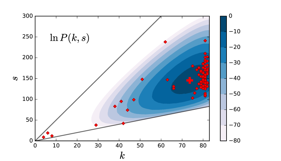
Figure 2: Contour plot for the joint log-density of states in the $k$-$s$ space for the grand-canonical ensemble with parameter values $\lambda=-0.3076$ and $\mu=-0.5842$. The red diamonds correspond to the dataset individual ego-networks and the red cross marks the empirical averages. The lines $s=k$ and $s=5k$ delimit the configuration minimum and maximum allowed total weight, respectively.

Next, let us compare the RS layer structure with the layer structure generated by the grand-canonical ensemble. Figure 3 shows the empirical layer degree and layer group sizes distributions along with the ensemble averages. Observing the RS layer distributions we find that the empirical averages of the three first layers lie within one standard deviation of the ensemble expected values, both for degrees, $k_{r}$ , and group sizes, $n_{r}$. On the other hand, the outermost layers degrees suffer from finite size effects. The discrepancy between ensemble and data is however corrected for the accumulated variables, $n_{r}$, which follow closely the ensemble scaling trend. Thus, condition (ii) is verified as well. Remarkably, the obtained value of $y=0.56$ is comparable with the empirical group size scaling for the outer layers, $\langle n_{4}/n_{5}\rangle=0.61$. Indeed, the approximation from Eq. (29) is better for the larger outer layers, where the correction factor $R_{r}$ tends to $1$, as shown on the inset of Fig. 3. We have also fitted the ensemble thermodynamic limit to the empirical data. Interestingly, despite the small size of the RS network, the grand-canonical ensemble results are barely distinguishable from its thermodynamic limit. Both ensembles average layer degrees and group sizes are equivalent, and only the variances of the outer layer degrees are slightly larger in the thermodynamic limit.

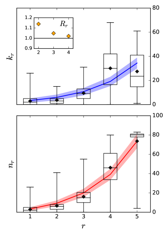
Figure 3: Layer degrees (top) and layer group sizes (bottom) distributions. The empirical distributions are represented by the black box-plots, where the box comprises the second and third quartiles, separated by the median line. The whiskers extend to the full distribution domain, and the averages are represented by the black diamonds. The colored lines join the corresponding ensemble averages, $\langle k_{r}\rangle$ (blue, left), and $\langle n_{r}\rangle$ (red, right) from the grand-canonical ensemble with parameters $N=84$, $x=0.74$ and $y=0.56$. Shaded regions comprise one standard deviation. The inset shows the numerical value of the micro-canonical correction factor $R_{r}=(1+\epsilon_{r})/(1+\epsilon_{r+1})$ which tends to $1$ for the outer layers.

V Discussion

We have proposed a grand-canonical ensemble as a null model for the hierarchical structure of social networks. The ensemble generates the observed nested structure of increasingly large layers of decreasing link weight. Moreover we show that, at least for the outer layers, a constant group size scaling between consecutive group pairings is possible only if the difference between costs of consecutive layers is constant. In the thermodynamic limit, that is, when the number of actors is large, the layer degrees are uncorrelated Poisson variables, which are related through the group size scaling, $y$. Interestingly, a recent paper providing more evidence on Dunbar’s theory shows the good fit of Poisson distributions to the layer-specific degree distributions Kordsmeyer et al. (2017). In the case of the dataset analyzed, after fitting the average values of the social bandwidth or resource $\langle s\rangle$ and degree $\langle k\rangle$, we find that typical samples of the ensemble are similar to the empirical ego-networks.

Interestingly, the statistical properties of our null model bear a strong formal relation to Bose-Einstein statistics. Such analogies have been reported earlier in the literature, e.g. the Bianconi-Barabási model for preferential attachment in networks Bianconi , where each node has a different energy level, and the role of particles is played by the links, and presenting Bose-Einstein condensation in a certain regime. Thus, it is relevant to ask whether our model can reach this phase, in which a larger fraction of the acquaintancies is accumulated at the lowest energy level, giving rise to a social network dominated by weak ties Meo.14 . We intend to consider this intriguing feature in future work.

The proposed null model succeeds at modeling survey social data, where the available categories could be directly used as representations of layers. However, in larger scale studies of ego-network social structure, layers are not given a priori, but rather inferred from the interaction patterns. The link weights usually represent frequency of interaction which acts as a proxy for emotional closeness, and ties are then clustered into discrete groups according to these weights Arnaboldi et al. (2012); Arnaboldi et al. (2013b); Dunbar et al. (2015); Carron et al. (2016). It is important to assert that we do not identify our link weights, or costs, with interaction frequency. Rather, we introduce the abstract notion of social resource, which can be spent in assigning discrete weights to the social ties. In order to justify this construction it can be argued that a limited social bandwidth may arise both from biological or temporal constraints, since maintaining a social relationship is costly Dunbar (1992); Gonçalves et al. (2011). Nevertheless our model remains uninformative about the psychological or sociological nature of that cost. The other main assumption of our model is the discrete nature of the layers. It is important to stress that we do not intend to neither justify nor provide any sort of explanation to their existence. We rather rely on the existing literature, where these layers have been consistently identified and even given specific names: the support clique of size $\raise 0.73193pt\hbox{$\scriptstyle\mathtt{\sim}$}5$, the sympathy group of size $\raise 0.73193pt\hbox{$\scriptstyle\mathtt{\sim}$}15$, the affinity group of size $\raise 0.73193pt\hbox{$\scriptstyle\mathtt{\sim}$}50$, and the total active network whose size equals the Dunbar’s number, $\raise 0.73193pt\hbox{$\scriptstyle\mathtt{\sim}$}150$ Zhou et al. (2005). Assigning the layers a constant cost is not only a convenient simplification, but has also a rather natural interpretation. Indeed the very existence of the layers would implicitly define different types of relationships for the ego. We simply consider that relationships within a given layer are similar precisely because they have the same cost. Then, the problem we focused on was to compute in how many different ways a given number of actors can be distributed in an ego’s network with the above mentioned restrictions. In our setting, once the layers, and the total average degree and social resource are fixed, the hierarchical structure emerges in a natural way, as the number of possible configurations with few strong and many weak links is much higher than configurations made of only strong or weak links. This result suggests that the observed hierarchical structure could be a consequence of the existence of an internal discrete categorization in which individuals organize different types of relationships. However, the reason why those categories or layers would exist in the first place remains unknown and shall be further explored.

Appendix A Cumulants of a quotient function

The cumulants of a quotient function $r(x,y)=x/y$ cannot be obtained directly from the partition function. However, they can be approximated by expanding $r(x,y)$ around the expected values, $\langle x\rangle$ and $\langle y\rangle$, as done in reference Sagarra et al. (2014). The mean and variance up to second order are given by

$$\centering\langle r\rangle\@add@centering =\frac{\langle x\rangle}{\langle y\rangle}\left[1+\frac{\langle y^{2}\rangle}{\langle y\rangle^{2}}-\frac{\langle xy\rangle}{\langle x\rangle\langle y\rangle}\right],$$ (31)

$$\sigma^{2}_{r} =\frac{\langle x\rangle^{2}}{\langle y\rangle^{2}}\left[\frac{\langle x^{2}\rangle}{\langle x\rangle^{2}}+\frac{\langle y^{2}\rangle}{\langle y\rangle^{2}}-\frac{2\langle xy\rangle}{\langle x\rangle\langle y\rangle}\right].$$ (32)

References

R. Dunbar, Journal of Human Evolution 22, 469 (1992).

R. Dunbar, Brain 9, 178 (1998).

B. Gonçalves, N. Perra, and A. Vespignani, PLoS ONE 6, 1 (2011).

G. Miritello, R. Lara, M. Cebrian, and E. Moro, Scientific Reports 3, 1950 EP (2013).

J. Stiller and R. Dunbar, Social Networks 29, 93 (2007).

S. G. B. Roberts and R. I. M. Dunbar, Evolution and Human Behavior 32, 186 (2011).

V. Arnaboldi, A. Guazzini, and A. Passarella, Computer Communications 36, 1130 (2013a).

J. Saramäki, E. A. Leicht, E. López, S. G. B. Roberts, F. Reed-Tsochas, and R. I. M. Dunbar, Proceedings of the National Academy of Sciences 111, 942 (2014).

W.-X. Zhou, D. Sornette, R. A. Hill, and R. I. M. Dunbar, Proceedings of the Royal Society of London B: Biological Sciences 272, 439 (2005).

R. Dunbar, V. Arnaboldi, M. Conti, and A. Passarella, Social Networks 43, 39 (2015).

R. I. M. Dunbar, Behavioral and Brain Sciences 16, 681–694 (1993).

B. Fuchs, D. Sornette, and S. Thurner, Scientific Reports 4, 6526 EP (2014), article.

V. Arnaboldi, M. Conti, A. Passarella, and F. Pezzoni, in Privacy, security, risk and trust (PASSAT), 2012 international conference on and 2012 international confernece on social computing (SocialCom) (IEEE, 2012), pp. 31–40.

V. Arnaboldi, M. Conti, A. Passarella, and F. Pezzoni, in INFOCOM, 2013 Proceedings IEEE (IEEE, 2013b), pp. 3459–3464.

P. M. Carron, K. Kaski, and R. Dunbar, Social Networks 47, 151 (2016).

N.J. Gotelli, G.R. Graves, Null models in Ecology, Smithsonian Inst. Press (1996).

O. Sagarra, C. J. Pérez Vicente, and A. Díaz-Guilera, Phys. Rev. E 88, 062806 (2013).

T. Squartini, F. Picciolo, F. Ruzzenenti, and D. Garlaschelli, Scientific Reports 3, e1003374 (2013).

O. Sagarra, C. J. Pérez Vicente, and A. Díaz-Guilera, Phys. Rev. E 92, 052816 (2015).

A. Antonioni, S. Bullock, M. Tomassini, REDS: an energy-constrained spatial social network model, in ALIFE 14: The fourteenth conference on the synthesis and simulation of living systems. The MIT Press (2014).

M. Jiménez-Martín, I. Tamarit, J. Rodríguez-Laguna, E. Korutcheva, ArXiv 1704.07428 (2017).

I. Tamarit, J.A. Cuesta, R.I.M. Dunbar, A. Sánchez, Proc. Nat. Acad. Sci. 115, 8316 (2018).

M. Kardar, Statistical physics of particles (Cambridge University Press, 2007).

L. Pitaevski, S. Stringari, Bose-Einstein condensation, Oxford Univ. Press (2003)

S. Grossmann, M. Holthaus, Phys. Rev. Lett. 79, 3557 (1997).

G. Bianconi. A.L. Barabási, Phys. Rev. Lett. 86, 5632 (2001).

E. T. Jaynes and G. L. Bretthorst, eds., Probability theory : the logic of science (Cambridge University Press, Cambridge, UK, New York, 2003), ISBN 0-521-59271-2.

J. Park and M. E. J. Newman, Phys. Rev. E 70, 066117 (2004).

D. Garlaschelli and M. I. Loffredo, Phys. Rev. E 78, 015101 (2008).

K. Anand and G. Bianconi, Phys. Rev. E 80, 045102 (2009).

A. Almaatouq, L. Radaelli, A. Pentland, and E. Shmueli, PLoS ONE 11, 1 (2016).

F. Wang and D. P. Landau, Phys. Rev. Lett. 86, 2050 (2001).

R. Fischer, J. C. Leitão, T. P. Peixoto, and E. G. Altmann, Phys. Rev. Lett. 115, 188701 (2015).

T. Kordsmeyer, P. Mac Carron, and R. Dunbar, Current Anthropology 58, 000 (2017).

O. Sagarra, F. Font-Clos, C. J. Pérez-Vicente, and A. Díaz-Guilera, EPL (Europhysics Letters) 107, 38002 (2014).

P. de Meo, E. Ferrara, G. Fiumara, A. Provetti, Comm. of the ACM 57, 78 (2014).