Cuts of Feynman Integrals in Baikov representation

Abstract

Based on the Baikov representation, we present a systematic approach to compute cuts of Feynman Integrals, appropriately defined in $d$ dimensions. The information provided by these computations may be used to determine the class of functions needed to analytically express the full integrals.

1 Introduction

It is almost seventy years from the time Feynman Integrals (FI) were first introduced Feynman:1949zx ; Dyson:1949bp ; Dyson:1949ha and forty-five years since the dimensional regularisation tHooft:1972tcz set up the framework for an efficient use of loop integrals in computing scattering matrix elements, and still the frontier of multi-scale multi-loop integral calculations (maximal both in number of scales and number of loops) is determined by the planar five-point two-loop on-shell massless integrals Gehrmann:2015bfy ; Papadopoulos:2015jft , recently computed. On the other hand, in order to keep up with the increasing experimental accuracy as more data is collected at the LHC, more precise theoretical predictions and higher loop calculations are required Andersen:2014efa .

In the last years our understanding of the reduction of one-loop amplitudes to a set of Master Integrals (MI), a minimal set of FI that form a basis, either based on unitarity methods Bern:1994cg ; Bern:1994zx ; Berger:2008sj or at the integrand level via the OPP method Ossola:2006us ; Ossola:2008xq , has drastically changed the way one-loop calculations are preformed resulting in many fully automated numerical tools (some reviews on the topic are AlcarazMaestre:2012vp ; Ellis:2011cr ; vanDeurzen:2015jmn ), making the next-to-leading order (NLO) approximation the default precision for theoretical predictions at the LHC. In the recent years, progress has been made also towards the extension of these reduction methods for two-loop amplitudes at the integral Gluza:2010ws ; Kosower:2011ty ; CaronHuot:2012ab ; Johansson:2012zv ; Johansson:2012sf ; Johansson:2013sda ; Sogaard:2013fpa ; Ita:2015tya ; Johansson:2015ava ; Mastrolia:2016dhn as well as the integrand Mastrolia:2011pr ; Badger:2012dp ; Mastrolia:2012wf ; Badger:2013gxa ; Papadopoulos:2013hra ; Badger:2015lda level. Two-loop MI are defined using the integration by parts (IBP) identities Chetyrkin:1981qh ; Tkachov:1981wb ; Laporta:2001dd , an indispensable tool beyond one loop. Contrary to the one-loop case, where MI have been known for a long time already 'tHooft:1978xw , a complete library of MI at two-loops is still missing. At the moment this is the main obstacle to obtain a fully automated NNLO calculation framework similar to the one-loop one, that will satisfy the precision requirements at the LHC Andersen:2014efa .

Many methods have been introduced in order to compute MI Smirnov:2012gma . The overall most successful one, is based on expressing the FI in terms of an integral representation over Feynman parameters, involving the two well-known Symanzik Polynomials $U$ and $F$ Bogner:2010kv . The introduction of the sector decomposition Hepp:1966eg ; Roth:1996pd ; Binoth:2000ps ; Binoth:2003ak ; Bogner:2007cr method resulted in a powerful computational framework for the numerical evaluation of FI, see for instance SecDec Borowka:2015mxa . An alternative is based on Mellin-Barnes representation Smirnov:1999gc ; Tausk:1999vh , implemented in Czakon:2005rk . Nevertheless, the most successful method to calculate multi-scale multi-loop FI is, for the time being, the differential equations (DE) approach Kotikov:1990kg ; Kotikov:1991pm ; Bern:1992em ; Remiddi:1997ny ; Gehrmann:1999as , which has been used in the past two decades to calculate various MI at two-loops and beyond. Following the work of refs. Goncharov:1998kja ; Remiddi:1999ew ; Goncharov:2001iea , there has been a building consensus that the so-called Goncharov Polylogarithms (GPs) form a functional basis for many MI. The so-called canonical form of DE, introduced by Henn Henn:2013pwa , manifestly results in MI expressed in terms of GPs . Nevertheless the reduction of a given DE to a canonical form is by no means fully understood. First of all, despite recent efforts Lee:2014ioa ; Meyer:2016slj ; Gituliar:2017vzm , and the existence of sufficient conditions that a given MI can be expressed in terms of GPs, no criterion, with practical applicability, that is at the same time necessary and sufficient has been introduced so far. Moreover, it is well known that when for instance enough internal masses are introduced, MI are not anymore expressible in terms of GPs, and in fact a new class of functions involving elliptic integrals is needed Adams:2015gva ; Bonciani:2016qxi .

In this paper we are studying another representation of FI introduced by Baikov Baikov:1996iu ; Baikov:1996rk ; Smirnov:2003kc ; Lee:2010wea ; Grozin:2011mt ; Lee:2013hzt . As we will see in Section 2, where we present a review of its derivation, it has several nice features, including its conceptual simplicity, a direct factorisation of kinematics and loop ‘topology’, incorporation of IBP identities in a straightforward manner. We also present, to the best of our knowledge for the first time, a consistent definition of the integration limits which will be important for the computation of cut integrals in $d$ dimensions. In Section 3 we elaborate on the loop-by-loop approach within the Baikov representation, that has a minimal number of integration variables for a given FI. In Section 4 we present a novel approach to obtain DE from the Baikov representation. In Section 5 we introduce the definition of the cut integral in Baikov representation, that satisfies the same DE and the same IBP identities as the uncut one Henn:2014qga , and we conjecture that computing the corresponding maximally cut integral Primo:2016ebd we may have a necessary and sufficient condition for the expression of the uncut integral in terms of GPs and when applied to the whole family of MI on the possibility to obtain a canonical form. Finally in Appendix A we present an alternative derivation of the Baikov representation for one- and two-loop FI and in Appendix B we collect several examples of maximally cut integrals in Baikov representation that support our findings.

2 The Baikov representation

In this section we introduce the Baikov representation following ref. Lee:2010wea ; Grozin:2011mt . An $L$-loop Feynman Integral with $E+1$ external lines can be written in the form

$${F_{{\alpha_{1}}...{\alpha_{N}}}}=\int{\left({\prod\limits_{i=1}^{L}{\frac{{{d^{d}}{k_{i}}}}{{i{\pi^{d/2}}}}}}\right)}\frac{1}{{D_{1}^{{\alpha_{1}}}...D_{N}^{{\alpha_{N}}}}}$$ (1)

with $N=\frac{{L\left({L+1}\right)}}{2}+LE$, $\alpha_{i}$ arbitrary integers, and $D_{a}$, $a=1,...,N$, inverse Feynman propagators, $P^{2}-M^{2}$, where $P$ represents, collectively, a linear combination of loop and external momenta and $M$ internal masses, as dictated by the Feynman Integral in consideration.

To be more specific, let us define $q_{i}=k_{i},(i=1,...,L)$ the loop momenta and $q_{L+i}=p_{i},(i=1,...,E)$, the independent external momenta, $M=L+E$ and $s_{ij}=q_{i}\cdot q_{j}$. Then

$${D_{a}}=\sum\limits_{i=1}^{L}{\sum\limits_{j=i}^{M}{A_{{}_{a}}^{ij}{s_{ij}}+{f_{a}}}}=\sum\limits_{i=1}^{L}{\sum\limits_{j=i}^{L}{A_{{}_{a}}^{ij}{k_{i}}\cdot{k_{j}}}}+\sum\limits_{i=1}^{L}{\sum\limits_{j=L+1}^{M}{A_{{}_{a}}^{ij}{k_{i}}\cdot{p_{j-L}}}}+{f_{a}},\,\,\,\,\,\,a=1,\ldots,N$$ (2)

where $f_{a}$ depend on external kinematics and internal masses. $A_{{}_{a}}^{ij}$ can be understood as an $N\times N$ matrix, with $a$ running obviously from $1$ to $N$ and with $(ij)$ taking also $N$ values as $i=1,\ldots,L$ and $j=i,\ldots,M$. The elements of the matrix $A_{{}_{a}}^{ij}$ are integer numbers taken from the set $\left\{-2,-1,0,+1,+2\right\}$. This matrix is characteristic of the corresponding Feynman graph and can, in a loose sense, be associated with the ‘topology’ of the graph. Then, by projecting each of the loop momenta $q_{i}=k_{i},(i=1,...,L)$ with respect to the space spanned by the external momenta involved plus a transverse component (for details see Grozin:2011mt ), we may write

$${F_{{\alpha_{1}}...{\alpha_{N}}}}=C_{N}^{L}{\left({G\left({{p_{1}},...,{p_{E}}}\right)}\right)^{\left({-d+E+1}\right)/2}}\int{\frac{{d{x_{1}}...d{x_{N}}}}{{x_{1}^{{\alpha_{1}}}...\,\,x_{N}^{{\alpha_{N}}}}}}P_{N}^{L}{\left({{x_{1}}-{f_{1}},...,{x_{N}}-{f_{N}}}\right)^{\left({d-M-1}\right)/2}}$$ (3)

with

$$C_{N}^{L}=\frac{{{\pi^{-L\left({L-1}\right)/4-LE/2}}}}{{\prod\nolimits_{i=1}^{L}{\Gamma\left({\frac{{d-M+i}}{2}}\right)}}}\det\left({A_{ij}^{a}}\right)$$ (4)

and

$$P_{N}^{L}\left({{x_{1}},{x_{2}},...,{x_{N}}}\right)={{{{{{G\left({{k_{1}},...,{k_{L}},{p_{1}},...,{p_{E}}}\right)}}}}}\Big{|}_{{s_{ij}}=\sum\limits_{a=1}^{N}{A_{ij}^{a}{x_{a}}\,\,\&\,\,\,{s_{ji}}={s_{ij}}}}}$$

with $G$ representing the Gram determinant, $G\left({{q_{1}},\ldots,{q_{n}}}\right)=\det\left({{q_{i}}\cdot{q_{j}}}\right)$ and $A_{ij}^{a}$ is the inverse of the topology matrix $A_{{}_{a}}^{ij}$. An alternative derivation of the Baikov representation for one- and two-loop FI is given in Appendix A.

Integration-by-parts identities can easily be accommodated in the Baikov representation. The generators of the IBP identities can be cast into the form

$$O_{ij}P_{N}^{L}=0$$ (5)

with the operators $O_{ij}$ given by ($i=1,\ldots,L$)

$$j\leq L\left({{q_{j}}={k_{j}}}\right)\,\,\,\,\,\,\,\,\,\,\,\,\,{O_{ij}}=d{\delta_{ij}}+\sum\limits_{a=1}^{N}{\sum\limits_{b=1}^{N}{\sum\limits_{m=1}^{M}{A_{a}^{mi}A_{mj}^{b}\left({1+{\delta_{mi}}}\right)\left({{x_{b}}-{f_{b}}}\right)}}}\frac{\partial}{{\partial{x_{a}}}}$$ (6)

and

$$j>L\left({{q_{j}}={p_{j-L}}}\right)\,\,\,\,\,\,\,\,{O_{ij}}=\sum\limits_{a=1}^{N}{\left({\sum\limits_{m=1}^{L}{\sum\limits_{b=1}^{N}{A_{a}^{mi}A_{mj}^{b}\left({1+{\delta_{mi}}}\right)\left({{x_{b}}-{f_{b}}}\right)+\sum\limits_{m=L+1}^{M}{A_{a}^{mi}{s_{mj}}}}}}\right)}\frac{\partial}{{\partial{x_{a}}}}$$ (7)

The derivation of the Baikov representation can easily be implemented in a computer algebra code.

We conclude this section by elaborating on the limits of the $x_{a}-$integrations in Eq. (3). In order to simplify the discussion, let us start with a generic one-loop configuration defined by

$${x_{1}}={k^{2}}-m_{1}^{2}\,,\quad{x_{2}}=\left({k+{p_{1}}}\right)^{2}-m_{2}^{2}\,,\quad\ldots\,,\quad{x_{N}}=\left({k+{p_{1}}+\ldots+{p_{N-1}}}\right)^{2}-m_{N}^{2}$$

Then consider the generic integral ($\alpha_{i}\geq 0$),

$$F_{\alpha_{1}\cdots\alpha_{N}}=C^{1}_{N}G\!\left(p_{1},\ldots,p_{N-1}\right)^{(N-d)/2}\int{\frac{{d{x_{1}}...d{x_{N}}}}{{x_{1}^{{\alpha_{1}}}...\,\,x_{N}^{{\alpha_{N}}}}}}{P^{1}_{N}}^{\left({d-N-1}\right)/2}$$ (8)

$$C^{1}_{N}=\frac{{{\pi^{-(N-1)/2}}}}{{{\Gamma\left({\frac{{d-N+1}}{2}}\right)}}}\left(\frac{1}{2}\right)^{N-1}$$ (9)

It is easy to verify that ${P^{1}_{N}}$ is a polynomial that is quadratic in the variables $x_{a}$ Smirnov:2003kc , and that obviously when $\alpha_{N}=0$, the external momentum $p_{N-1}$ decouples, so that

$${F_{{\alpha_{1}}...{\alpha_{N-1}}{0}}} = {C^{1}_{N}}G\!\left(p_{1},\ldots,p_{N-1}\right)^{(N-d)/2}\int{\frac{{d{x_{1}}...d{x_{N-1}}}}{{x_{1}^{{\alpha_{1}}}...\,\,x_{N-1}^{{\alpha_{N-1}}}}}\int\limits_{x_{N}^{-}}^{x_{N}^{+}}{d{x_{N}}}}{P^{1}_{N}}^{\left({d-N-1}\right)/2}$$

$$= C^{1}_{N-1}G\!\left(p_{1},\ldots,p_{N-2}\right)^{(N-1-d)/2}\int{\frac{{d{x_{1}}...d{x_{N-1}}}}{{x_{1}^{{\alpha_{1}}}...\,\,x_{N-1}^{{\alpha_{N-1}}}}}}{P^{1}_{N-1}}^{\left({d-\left(N-1\right)-1}\right)/2}$$

where ${P^{1}_{N}}\left({x_{N}^{+}}\right)={P^{1}_{N}}\left({x_{N}^{-}}\right)=0$ and

$$\int\limits_{x_{N}^{-}}^{x_{N}^{+}}{d{x_{N}}{P^{1}_{N}}^{\left({d-N-1}\right)/2}} = \frac{{2{\pi^{1/2}}\Gamma\left({\frac{{d-N+1}}{2}}\right)}}{{\Gamma\left({\frac{{d-N+2}}{2}}\right)}}G\left(p_{1},\ldots,p_{N-1}\right)^{(d-N)/2}G\left(p_{1},\ldots,p_{N-2}\right)^{(N-1-d)/2}$$

$$\times {P^{1}_{N-1}}^{\left({d-\left({N-1}\right)-1}\right)/2}$$

using $P_{N}^{1}=\frac{1}{4}G\left({{p_{1}},\ldots,{p_{N-2}}}\right)\left({x_{N}^{+}-{x_{N}}}\right)\left({{x_{N}}-x_{N}^{-}}\right)$ and ${\left({x_{N}^{+}-x_{N}^{-}}\right)^{2}}=16\frac{{G\left({{p_{1}},\ldots,{p_{N-1}}}\right)}}{{G{{\left({{p_{1}},\ldots,{p_{N-2}}}\right)}^{2}}}}P_{N-1}^{1}$. This can be repeated straightforwardly for all variables except $x_{1}=k^{2}-m_{1}^{2}$ whose integration limits are simply derived from the $k-$modulus integration limits. The generalisation to the two-loop case is straightforward, with the integration at each step performed over the $x-$variables involving a given external momentum, and the last ones derived by the corresponding $k_{1}-$ and $k_{2}-$modulus integration limits. We have checked both analytically and numerically that the limits, as defined above, reproduce the known results for several examples at one and two loops.

3 The loop-by-loop approach

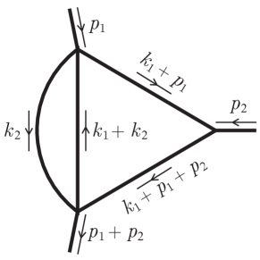
Figure 1: The two-loop three-point graph considered in the text.

At one loop the number of Baikov variables and the number of propagators of a generic Feynman Integral can be the same. At higher loops this is not the case anymore. Consider for instance the double-box, with $E=3$ independent external momenta and $L=2$, giving $N=9$ and $M=5$. In that case we have to integrate over nine variables whereas the scalar double-box graph has only seven denominators. Of course this mismatch is the origin of the well known irreducible scalar products (ISP) appearing for $L\geq 2$. It is eventually desirable to have a representation with the minimal number of integration variables. This can be achieved by considering the projection over the space spanned by the external momenta of each loop integration momentum separately. As an example to illustrate the concept, consider the two-loop three-point Feynman Integral of Figure 1. The standard Baikov representation is based on the following set of seven inverse propagators

$$x_{1} =k_{1}^{2}-m_{1}^{2} x_{2} =(k_{1}+p_{1})^{2}-m_{2}^{2} x_{3} =(k_{1}+p_{1}+p_{2})^{2}-m_{3}^{2}$$

$$x_{4} =k_{2}^{2}-m_{4}^{2} x_{5} =(k_{2}-p_{1})^{2}-m_{5}^{2} x_{6} =(k_{2}-p_{1}-p_{2})^{2}-m_{6}^{2}$$ (11)

$$x_{7} =(k_{1}+k_{2})^{2}-m_{7}^{2}\!\!\!\!\!\!\!\!\!\!\!\!\!\!\!\!\!\!\!\!$$

$${F_{0111001}}=C_{3}^{2}{\left({G\left({{p_{1}},{p_{2}}}\right)}\right)^{-\left({d-3}\right)/2}}\int{\frac{{d{x_{1}}\ldots d{x_{7}}}}{{{x_{2}}{x_{3}}{x_{4}}{x_{7}}}}{{\left({P_{3}^{2}}\right)}^{\left({d-5}\right)/2}}}$$ (12)

For the integral ${F_{0111001}}$, in the loop-by-loop approach one can consider the $k_{1}$ and $k_{2}$ integrations separately. Starting with $k_{2}$ integration it is easy to see that we have a two-point function with external momentum $k_{1}$.

$${F_{0111001}}=\int{\frac{{{d^{d}}{k_{1}}}}{{i{\pi^{d/2}}}}\frac{{{d^{d}}{k_{2}}}}{{i{\pi^{d/2}}}}\frac{1}{{{x_{2}}{x_{3}}{x_{4}}{x_{7}}}}}=C_{2}^{1}\int{\frac{{{d^{d}}{k_{1}}}}{{i{\pi^{d/2}}}}\frac{1}{{{x_{2}}{x_{3}}}}{{\left({{x_{1}}+m_{1}^{2}}\right)}^{-\left({d-2}\right)/2}}\int{\frac{{d{x_{4}}d{x_{7}}}}{{{x_{4}}{x_{7}}}}}{{\left({P_{2}^{1}}\right)}^{\left({d-3}\right)/2}}}$$ (13)

Then for the $k_{1}$ integration we have a three-point integral with two external momenta $p_{1}$ and $p_{2}$.

$${F_{0111001}}=C_{2}^{1}C_{3}^{1}{\left({G\left({{p_{1}},{p_{2}}}\right)}\right)^{-\left({d-3}\right)/2}}\int{\frac{{d{x_{1}}d{x_{2}}d{x_{3}}d{x_{4}}d{x_{7}}}}{{{x_{2}}{x_{3}}{x_{4}}{x_{7}}}}{{\left({{x_{1}}+m_{1}^{2}}\right)}^{-\left({d-2}\right)/2}}{{\left({P_{3}^{1}}\right)}^{\left({d-5}\right)/2}}}{\left({P_{2}^{1}}\right)^{\left({d-3}\right)/2}}$$ (14)

Notice that the same result can be obtained from Eq. (12) integrating out $x_{5}$ and $x_{6}$, as detailed at the end of the previous section. Nevertheless, the loop-by-loop approach offers an alternative way of obtaining a minimal number of integration variables.

4 Deriving differential equations

It is instructive to study the way differential equations with respect to external kinematics and masses can be obtained in Baikov representation. Differential equations are usually written in terms of external kinematical invariants, $s_{ij}=(p_{i}+p_{j})^{2}$ and internal masses, $m_{i}^{2}$. In the standard approach, since the integral in the momentum-space representation is not an explicit function of the kinematical invariants, derivatives with respect to external momenta, $p_{j}^{\mu}\frac{\partial}{{\partial p_{i}^{\mu}}}$, are used. In Baikov representation though, the dependence on external kinematical invariants and internal masses is explicit. Indeed in Eq. (3), it is easy to identify two terms that depends on the external kinematics and/or masses, namely the overall factor $G\left(p_{1},\ldots,p_{E}\right)^{\left({-d+E+1}\right)/2}$ and the Baikov polynomial $P_{N}^{L}$ itself. The differentiation of the first factor causes no problem since the result is expressed in terms of the original integral. For the Baikov polynomial this is not so, since the derivative introduces a different integrand that is not directly expressible in terms of FI, Eq. (1). To be more specific, let us denote by $X$ a generic kinematical variable, for instance a Mandelstam invariant $X=\left(p_{i}+p_{j}\right)^{2}$ or an internal mass $X=m_{i}^{2}$. Then

$$\frac{\partial}{{\partial X}}{F_{{\alpha_{1}}...{\alpha_{N}}}} = \left({\frac{{-d+E+1}}{2}}\right)\left(\frac{1}{G}\frac{{\partial G}}{{\partial X}}\right){F_{{\alpha_{1}}...{\alpha_{N}}}}$$

$$+ C_{N}^{L}{G^{\left({-d+E+1}\right)/2}}\int{\frac{{d{x_{1}}...d{x_{N}}}}{{x_{1}^{{\alpha_{1}}}...\,\,x_{N}^{{\alpha_{N}}}}}}{P_{N}^{L}}^{\left({d-M-1}\right)/2}\left[{\left({\frac{{d-M-1}}{2}}\right)\frac{1}{{P_{N}^{L}}}\frac{{\partial P_{N}^{L}}}{{\partial X}}}\right]$$

where $G$ is used for ${G\left({{p_{1}},...,{p_{E}}}\right)}$. Based on the fact that the derivatives $\frac{{\partial P_{N}^{L}}}{{\partial X}},\frac{{\partial P_{N}^{L}}}{{\partial{x_{a}}}}$ are polynomials in $x_{a}$, the idea is to turn the derivative with respect to $X$ into derivatives with respect to $x_{a}$. This can be achieved by the equation, known as the syzygy equation Larsen:2015ped ; Georgoudis:2016wff ,

$$b\frac{{\partial P_{N}^{L}}}{{\partial X}}+\sum\limits_{a}{{c_{a}}\frac{{\partial P_{N}^{L}}}{{\partial{x_{a}}}}}=0$$ (16)

with $b$ and $c_{a}$ being polynomials in $x_{a}$.

Assuming that a solution of this equation has been found such that $b$ is independent of $x_{a}$ (eventually depending on external kinematics and internal masses and not identical to zero), we have

$$\frac{\partial}{{\partial X}}{F_{{\alpha_{1}}...{\alpha_{N}}}} = \left({\frac{{-d+E+1}}{2}}\right)\frac{1}{G}\frac{{\partial G}}{{\partial X}}{F_{{\alpha_{1}}...{\alpha_{N}}}}$$ (17)

$$+ C_{N}^{L}{G^{\left({-d+E+1}\right)/2}}\int{\frac{{d{x_{1}}...d{x_{N}}}}{{x_{1}^{{\alpha_{1}}}...\,\,x_{N}^{{\alpha_{N}}}}}}\left(-{\sum\limits_{a}{\frac{{{c_{a}}}}{b}\frac{\partial}{{\partial{x_{a}}}}P{{{}_{N}^{L}}^{\left({d-M-1}\right)/2}}}}\right)$$

Then integrating by parts the second term in the rhs of the above equation and assuming that surface terms are vanishing (a standard assumption through Baikov representation) we get

$$\frac{\partial}{{\partial X}}{F_{{\alpha_{1}}...{\alpha_{N}}}} = \left({\frac{{-d+E+1}}{2}}\right)\frac{1}{G}\frac{{\partial G}}{{\partial X}}{F_{{\alpha_{1}}...{\alpha_{N}}}}$$

$$+ C_{N}^{L}{G^{\left({-d+E+1}\right)/2}}\int{d{x_{1}}...d{x_{N}}}{P_{N}^{L}}^{\left({d-M-1}\right)/2}\left\{{\sum\limits_{a}{\frac{\partial}{{\partial{x_{a}}}}\left({\frac{{{c_{a}}}}{b}\frac{1}{{x_{1}^{{\alpha_{1}}}...\,\,x_{N}^{{\alpha_{N}}}}}}\right)}}\right\}$$

The term in the curly bracket is easily seen to be a sum of terms of the form

$$\frac{1}{{x_{1}^{{{\alpha^{\prime}}_{1}}}...\,\,x_{N}^{{{\alpha^{\prime}}_{N}}}}}$$

The powers $\alpha^{\prime}_{a}$ depend on the actual form of the solution of the syzygy equation, Eq. (16). The result is as expected

$$\frac{\partial}{{\partial X}}{F_{{\alpha_{1}}...{\alpha_{N}}}}=\sum\limits_{i}{{R_{i}}}\,\,{F_{\alpha_{1}^{\left(i\right)}...\alpha_{N}^{\left(i\right)}}}$$ (19)

with coefficients $R_{i}$ that are rational functions of the space-time dimension $d$, the external kinematics and the internal masses. The rhs of the above equation contains integrals that are in general not MI. We have verified in numerous examples, that after applying a standard IBP reduction to MI for the rhs of the above equation, the resulting differential equations for the MI are the same as those obtained with the standard approach. It is still interesting to note that the initial form, Eq. (19), is generally not.

5 Cutting Feynman Integrals

Cutting FI in the Baikov representation has a very natural definition. Indeed we define an $n-$cut as follows

$${F}_{{\alpha_{1}}...{\alpha_{N}}}|_{n\times\text{cut}}\equiv C_{N}^{L}{\left(G\right)^{\left({-d+E+1}\right)/2}}\left({\prod\limits_{a=n+1}^{N}{\int{d{x_{a}}}}}\right)\left({\prod\limits_{c=1}^{n}{\oint\limits_{{x_{c=0}}}{d{x_{c}}}}}\right)\frac{1}{{x_{1}^{{\alpha_{1}}}\ldots x_{N}^{{\alpha_{N}}}}}{P_{N}^{L}}^{\left({d-M-1}\right)/2}$$ (20)

where the Baikov variables $\{x_{a}:a=1,...,N\}$ have been divided in two subsets, containing $n$ cut propagators and $(N-n)$ uncut ones. The cut operation defined above is operational in any space-time dimension $d$ and for any FI given by Eq. (1). Notice that the definition of the cut, Eq. (20), is not identical to the traditional unitarity cut, see for instance Section 8.4 of ref. Veltman:1994wz , due to the lack of the $\theta$-function constraint on the energy, and therefore it is not directly related to the discontinuity of the FI Abreu:2014cla ; Abreu:2015zaa .

Let us now consider a set of MI, ${F_{i}}\equiv{F_{\alpha_{1}^{\left(i\right)}...\alpha_{N}^{\left(i\right)}}}$, $i=1,...,I$, satisfying a system of DE, with respect to variables $X_{j}$,

$$\frac{\partial}{{\partial{X_{j}}}}{F_{i}}=\sum\limits_{l=1}^{I}{M_{il}^{\left(j\right)}{F_{l}}}$$ (21)

with matrices $M^{(j)}$ depending on kinematical variables, internal masses, and the space-time dimension, $d$. Since the derivation of DE in Section 4 is insensitive to the cut operation, as defined in Eq. (20), we may immediately write

$$\frac{\partial}{\partial X_{j}}F_{i}|_{n\times\text{cut}}=\sum_{l=1}^{I}M_{il}^{(j)}F_{l}|_{n\times\text{cut}}$$ (22)

with $F|_{n\times\text{cut}}$ representing an arbitrary $n-$cut: in other words, the cut integrals satisfy the same DE as the uncut ones. Of course for a given $n-$cut many of the MI that are not supported on the corresponding cut vanish identically. Nevertheless, Eq. (22) remains valid. Especially for the maximally cut integrals defined so that $n$ is equal to the number of propagators (with $\alpha_{i}>0$) of the integral, all integrals not supported on the cut vanish and the resulting DE is restricted to its homogeneous part. Evaluating the maximally cut MI provides therefore a solution to the homogeneous equation Henn:2014qga ; Primo:2016ebd . Non-maximally cut integrals, on the other hand, can resolve non-homogenous parts of the DE as well Henn:2014qga .

One important implication is that cut and uncut integrals, although very different in many respects, as for instance their structure in $\epsilon-$expansion ($\epsilon\equiv(4-d)/2$), they are expressed in terms of the same class of functions. This is particularly important if we want to know a priori if a system of DE can be solved, for instance, in terms of Goncharov Polylogarithms, or if the solution contains a larger class of functions including, for instance Elliptic Integrals.

In Appendix B we have collected several results of maximally cut MI: in B.1 we study a double-box with a massive loop, and find that it is expressible in terms of Polylogarithmic functions; in B.2 we study two-loop sunset graph and show that only the fully massive one is elliptic; in B.3 we show how results can be obtained beyond $d=4$ and verified that certain maximally cut integrals as well as certain combinations of maximally cut integrals are expressed in terms of GPs in exactly the same way as their uncut counterparts; in B.4 we show that the cut of the elliptic box-triangle integral Bonciani:2016qxi is elliptic as well, and finally in B.5 we study the elliptic double-box Bonciani:2016qxi , and verify that the Elliptic Integrals only enter through its sub-topologies.

6 Discussion and Outloook

In this paper we have studied properties of Feynman integrals in Baikov representation. We have shown how to determine the limits of integration and how to obtain DE with respect to external kinematics and internal masses. We have introduced also a loop-by-loop approach in constructing the Baikov representation, so that for certain FI a smaller number of integration variables is obtained. Then we provided a definition of a cut integral, operational in $d$ dimensions, and show that a cut integral satisfies the same system of DE as the uncut, original integral. We have shown how to compute the simplest, i.e. maximally, cut integral in Baikov representation, and give explicit results for several cases.

Based on the fact that cut integrals satisfy the same system of DE as the full, uncut integrals we have verified that their analytic expressions are given in terms of the same class of functions, such as Goncharov Polylogarithms or Elliptic Integrals. We have therefore arrived at the conclusion that in a family of MI satisfying a given system of DE, the study of the maximally cut integrals for all its members can provide a necessary and sufficient criterion for the existence of a canonical form of the DE, and in the case when such a canonical form does not exist, it provides solutions of the homogeneous parts of the system of DE (see also ref. Henn:2014qga ; Primo:2016ebd ). An application of these ideas to non-planar pentabox integrals will be discussed elsewhere.

Baikov representation is well suited for these considerations, drastically simplifying the computation of cut integrals for arbitrary external momenta and internal masses. It is still an open question if it can also be used to actually compute the MI. To this end, an algorithm, allowing the resolution of singularities in $\epsilon$, needs to be devised. It remains to be seen if this is possible and more importantly what kind of integral representations for the individual terms in this expansion such an algorithm produces.

Acknowledgements

We gratefully acknowledge fruitful discussions with P. A. Baikov, V. A. Smirnov, M. Czakon, R. N. Lee, E. Panzer, C. Anastasiou, K. J. Larsen, J. Henn and C. Duhr during various stages of this project. This research was supported through the Initial Training Network HiggsTools under contract PITN-GA-2012-316704.

Appendix A Alternative derivation of the Baikov representation

In this appendix we will show an alternative derivation of the Baikov representation of Feynman integrals, complementary to the one given in section 2 in the main text.

We start from Eq. (1) for the one-loop case

$$F_{\alpha_{1}\ldots\alpha_{N}}=\int\!\frac{d^{d}k}{i\pi^{d/2}}\,\frac{1}{D_{1}^{\alpha_{1}}\cdots D_{N}^{\alpha_{N}}}$$ (23)

The integrand $(D_{1}^{\alpha_{1}}\cdots D_{N}^{\alpha_{N}})^{-1}$ depends on $E$ independent external momenta, which allows us to split the integration into an $E$-dimensional “parallel” subspace $k_{||}$ and a $(d-E)$-dimensional “orthogonal” subspace $k_{\perp}$. Notice that the integrand depends on the orthogonal directions only through $k_{\perp}^{2}$, allowing us to perform the angular part of the integral over the orthogonal space

$$F_{\alpha_{1}\ldots\alpha_{N}}=\frac{\pi^{-E/2}}{i\,\Gamma((d-E)/2)}\int\!\frac{\lambda^{(d-E-2)/2}}{D_{1}^{\alpha_{1}}\cdots D_{N}^{\alpha_{N}}}\,d^{E}k_{||}d\lambda$$ (24)

where we define $\lambda\equiv k_{\perp}^{2}$.

We change now to a different set of variables $\varsigma_{i}\equiv k\cdot p_{i}$ which is equivalent to $s_{1,E+i}$ from section 2. Defining $G$ as the Gram determinant of the external momenta, it is not hard to realize that $d^{E}k_{||}=-(-G)^{-1/2}d^{E}\varsigma$, and we now want to change the integration to the set of Baikov variables $x$. Using the same argument as in section 2, we get that $d^{E}k_{||}d\lambda=\det(A^{-1})d^{E+1}x$ where $A$ is the matrix defined in Eq. (2), and we see that $\det(A^{-1})=\pm 2^{-E}$ depending on the sign of the external momenta in the definition of the loop momenta. Putting this together, yields

$$F_{\alpha_{1}\ldots\alpha_{N}}=\frac{i\pi^{-E/2}}{\Gamma((d-E)/2)}\frac{\det(A^{-1})}{\sqrt{-G}}\int\!\frac{\lambda^{(d-E-2)/2}}{x_{1}^{\alpha_{1}}\cdots x_{N}^{\alpha_{N}}}\,d^{E+1}x$$ (25)

If additionally we use that $\lambda=P/G$ where $P$ – the Baikov polynomial – is given as the Gram determinant of the full set of momenta $\{q\}=\{k,p_{1},\ldots,p_{E}\}$, we see that Eq. (25) is equivalent to Eq. (3) in the one-loop case. The above derivation can be straightforwardly generalised for any numbers of loops.

The loop-by-loop case

We may now go through the same procedure as above, loop by loop, for a two-loop process. A traditional Baikov representation of a two-loop Feynman integral with $E$ independent external momenta would involve $3+2E$ integrations, but in most cases it is possible to get the number further down. Each individual loop will in general be dependent only on a subset of the $E$ external momenta. Let us denote with $k_{2}$ the loop momentum of the loop with the smallest such subset, and the size of that subset $E_{2}-1$. This means that the integrand of this loop depends on $E_{2}$ different momenta including $k_{1}$. Performing the transverse angular part of the $k_{2}$ integration individually with the method leading up to Eq. (24), gives

$$F^{\text{two-loop}}_{\alpha_{1}\ldots\alpha_{N}}=\frac{-\pi^{-(E_{2}+d)/2}}{\Gamma((d-E_{2})/2)}\int\!\frac{\lambda_{22}^{(d-E_{2}-2)/2}}{D_{1}^{\alpha_{1}}\cdots D_{N}^{\alpha_{N}}}\;\;d^{E_{2}}{k_{2}}_{||}d\lambda_{22}d^{d}k_{1}$$ (26)

where $\lambda_{22}={k_{2}}_{\perp}^{2}$.

The integrand now depends on all the external momenta, so the transverse angular part of the $k_{1}$ integration may be done, leaving $E+E_{2}+2$ integrations in total. So only in the cases where both loops depend on $E$ external momenta (so $E_{2}=E+1$) the number of integrations will be equal to that of the standard Baikov approach, otherwise it will be smaller.

Changing integration variables from $k_{||}$ to $\varsigma$ and from $\varsigma$ and $\lambda$ to the Baikov variables $x$, our result for the two-loop case in the loop-by-loop approach is written as

$$F^{\text{two-loop}}_{\alpha_{1}\ldots\alpha_{N}}=\frac{-\pi^{-(E+E_{2})/2}}{\Gamma((d-E)/2)\,\Gamma((d-E_{2})/2)}\frac{\det(A^{-1})}{\sqrt{-G_{1}}}\int\!\frac{\lambda_{11}^{(d-E-2)/2}\lambda_{22}^{(d-E_{2}-2)/2}}{\sqrt{-G_{2}}\;x_{1}^{\alpha_{1}}\cdots x_{N}^{\alpha_{N}}}\,d^{E+E_{2}+2}x$$ (27)

with $G_{1}$ the Gram determinant of the $E$ external momenta and $G_{2}$ the Gram determinant of the $E_{2}$ different momenta including $k_{1}$.

Appendix B Examples of cuts performed in Baikov variables

In the appendix we will go through several examples of maximally cut Feynman integrals.

B.1 Double-box with massive loop

As a first example we will do a double-box with one massive loop. That integral is given as

$$F_{\text{double-box}} =\int\!\frac{d^{d}k_{1}}{i\pi^{d/2}}\frac{d^{d}k_{2}}{i\pi^{d/2}}\frac{1}{x_{1}x_{2}x_{3}x_{4}x_{5}x_{6}x_{7}}$$ (28)

with

$$x_{1} =k_{1}^{2}-m^{2} x_{2} =(k_{1}+p_{1})^{2}-m^{2}\quad x_{3} =(k_{1}+p_{1}+p_{2})^{2}-m^{2}$$

$$x_{4} =(k_{2}+p_{1}+p_{2})^{2}\quad x_{5} =(k_{2}-p_{4})^{2} x_{6} =k_{2}^{2}$$

$$x_{7} =(k_{1}-k_{2})^{2}-m^{2} x_{8} =(k_{1}-p_{4})^{2}-m^{2}$$ (29)

where $x_{8}$ is needed for later. Using the loop-by-loop approach, Eq. (30), we may perform the angular parts of the integral, leaving integrals over the eight Baikov variables

$$F_{\text{double-box}}=\frac{-\pi^{-3}}{\Gamma^{2}((d-3)/2)}\frac{\det(A^{-1})}{\sqrt{-G_{1}}}\int\!\frac{\lambda_{11}^{(d-5)/2}\lambda_{22}^{(d-5)/2}}{\sqrt{-G_{2}}\;x_{1}\cdots x_{7}}\,d^{8}x$$ (30)

The various quantities are

$$\lambda_{11} =\bigg{(}4m^{2}st(s+t)+2st\Big{(}2x_{1}x_{3}-x_{1}x_{2}-x_{2}x_{3}+t(x_{1}+x_{3})-(x_{1}-2x_{2}+x_{3})x_{8}\Big{)}$$

$$\;\;\;-s^{2}\Big{(}t^{2}+(x_{2}-x_{8})^{2}-2t(x_{2}+x_{8})\Big{)}-t^{2}(x_{1}-x_{3})^{2}\bigg{)}/\Big{(}4st(s+t)\Big{)}$$ (31)

$$\lambda_{22} =-\bigg{(}4m^{2}s\Big{(}-(sx_{5})+(x_{4}-x_{5})(x_{5}-x_{6})\Big{)}+\Big{(}x_{3}(-x_{5}+x_{6})+s(x_{5}-x_{7})\Big{)}^{2}$$

$$\;\;+2\Big{(}x_{3}(x_{4}-x_{6})(-x_{5}+x_{6})-s^{2}(x_{5}+x_{7})+s(x_{4}x_{5}-2x_{4}x_{6}+x_{5}x_{6}+x_{3}(x_{5}+x_{6})$$

$$\;\;+(x_{4}-2x_{5}+x_{6})x_{7})\Big{)}x_{8}+\Big{(}s^{2}+(x_{4}-x_{6})^{2}-2s(x_{4}+x_{6})\Big{)}x_{8}^{2}$$

$$\;\;+x_{1}^{2}(x_{4}-x_{5})^{2}+2x_{1}\Big{(}s(-2x_{3}x_{5}+(x_{4}-x_{5})(x_{5}-x_{7})+(x_{4}+x_{5})x_{8})$$ (32)

$$\;\;+(x_{4}-x_{5})(x_{3}(x_{5}-x_{6})+(-x_{4}+x_{6})x_{8})\Big{)}\bigg{)}/\Big{(}4s(m^{2}s+(x_{1}-x_{8})(x_{3}-x_{8})+sx_{8})\Big{)}$$

$$G_{1}=-st(s+t)/4$$

$$G_{2}=-s\Big{(}m^{2}s+x_{1}(x_{3}-x_{8})+x_{8}(s-x_{3}+x_{8})\Big{)}/4$$ (33)

$$\det\big{(}A^{-1}\big{)}=1/64$$

and $s={\left({{p_{1}}+{p_{2}}}\right)^{2}},t={\left({{p_{1}}+{p_{4}}}\right)^{2}},s>0,t<0,s+t>0,{m^{2}}>0$.

Inserting all this, cutting the seven propagators, expanding in $\epsilon$, and renaming $x_{8}$ to $z$, gives

$$F_{\text{double-box}|7\times\text{cut}} =\frac{1}{4\pi^{4}}\frac{1}{s}\,\int_{r_{-}}^{r_{+}}\!dz\frac{1}{z\sqrt{P(z)}}\;+\;\mathcal{O}(\epsilon)$$ (34)

where

$$P(z) =-4m^{2}s^{2}t-4m^{2}st^{2}+s^{2}t^{2}-2s^{2}tz+s^{2}z^{2}$$ (35)

and $r_{\mp}$ are the two roots of $P(z)$. The result is

$$F_{\text{double-box}|7\times\text{cut}} =\frac{1}{4\pi^{4}}\;\frac{i\pi}{s\sqrt{st(st-4m^{2}(s+t))}}\;+\;\mathcal{O}(\epsilon).$$ (36)

In fact we have computed also the order $\epsilon$ which is given in terms of weight 2 functions, but since it is quite extensive we give the result for another MI, defined as follows,

$$F_{\text{double-box-N}} =\int\!\frac{d^{d}k_{1}}{i\pi^{d/2}}\frac{d^{d}k_{2}}{i\pi^{d/2}}\frac{x_{8}}{x_{1}x_{2}x_{3}x_{4}x_{5}x_{6}x_{7}}$$ (37)

whose expression is simpler,

$$I\equiv-4i{\pi^{3}}{e^{2{\gamma_{E}}\epsilon}}{s^{2+\epsilon}}{\left({-t}\right)^{-\epsilon}}{\left({s+t}\right)^{-\epsilon}}{\left({{m^{2}}}\right)^{3\epsilon}}F_{\text{double-box-N}|7\times\text{cut}}$$ (38)

$$I = 1-\epsilon\log\left({\frac{{-4{t^{3}}{{\left({s+t}\right)}^{2}}{{\left({\sqrt{{Y_{+}}}+\sqrt{{Y_{-}}}}\right)}^{4}}}}{{{m^{2}}{{\left({\sqrt{{X_{+-}}}+\sqrt{{X_{--}}}}\right)}^{2}}{{\left({\sqrt{{X_{-+}}}+\sqrt{{X_{++}}}}\right)}^{2}}}}}\right)+\mathcal{O}(\epsilon^{2})$$

$${X_{\pm\pm}} = ms\sqrt{t(s-4{m^{2}})(s+t)}\pm 4{m^{2}}t(s+t)\pm m\sqrt{st\left({s+t}\right)}(s+2t)$$ (39)

$${Y_{\pm}} = 2m\sqrt{s+t}\pm\sqrt{st}$$

suggesting that the solution is expressible in terms of logarithmic/polylogarithmic functions.

B.2 The sunset

We will here go through the same considerations for the well-studied sunset-integral Adams:2015gva . The integral is given as

$$F_{\text{sunset}} =\int\!\frac{d^{d}k_{1}\,d^{d}k_{2}}{\big{(}i\pi^{d/2}\big{)}^{2}}\frac{1}{x_{1}x_{2}x_{3}}$$ (40)

with

$$x_{1} =(k_{1}-p)^{2}-m_{1}^{2} x_{2} =k_{2}^{2}-m_{2}^{2} x_{3} =(k_{1}-k_{2})^{2}-m_{3}^{2} x_{4} =k_{1}^{2}.$$ (41)

Using the loop-by-loop approach, we get

$$F_{\text{sunset}} =\frac{-\pi^{-1}}{\Gamma^{2}((d-1)/2)}\frac{\det(A^{-1})}{\sqrt{-G_{1}}}\int\!\frac{\lambda_{11}^{(d-3)/2}\lambda_{22}^{(d-3)/2}}{\sqrt{-G_{2}}\;x_{1}x_{2}x_{3}}\,d^{4}x$$ (42)

with

$$\lambda_{22}=\lambda(x_{4},m_{2}^{2},m_{3}^{2})\;\;\;\;\;\;\lambda_{11}=\lambda(s,x_{4},m_{1}^{2})$$ (43)

$\lambda(s_{1},s_{2},s_{3})\equiv s_{1}^{2}+s_{2}^{2}+s_{3}^{2}-2s_{1}s_{2}-2s_{2}s_{3}-2s_{3}s_{1}$, is the Källén function and $s=p^{2}$. Performing the triple cut gives Remiddi:2016gno ,

$$F_{\text{sunset}|3\times\text{cut}} \varpropto s^{-1+\epsilon}\int dx_{4}x_{4}^{-1+\epsilon}\left(\lambda_{11}\lambda_{22}\right)^{1/2-\epsilon}$$ (44)

Expanding in $\epsilon$

$$F_{\text{sunset}|3\times\text{cut}} \varpropto s^{-1}\int dx_{4}x_{4}^{-1}\left(\lambda_{11}\lambda_{22}\right)^{1/2}+\mathcal{O}(\epsilon)$$ (45)

it is easily seen that this is an integral over the square-root of a quartic polynomial Remiddi:2016gno , which yields elliptic integrals, and such functions are indeed present in the result for the full sunset integral as well. On the other hand, if any of the masses vanish, the square root partially factorises, and the result is expressible in terms of polylogarithmic functions.

Notice, that the extra cut over $x_{4}$ ($m_{2}>m_{3}$), after expanding in $\epsilon$,

$$\oint\limits_{{x_{4}}=0}{}dx_{4}x_{4}^{-1}\left(\lambda_{11}\lambda_{22}\right)^{1/2} =(s-m_{1}^{2})(m_{2}^{2}-m_{3}^{2})$$ (46)

yields a rational term at order $\mathcal{O}(\epsilon^{0})$, which seems to contradict our previous findings, Eq. (45), as well as the known result for the full integral Adams:2015gva . Nevertheless, it is easy to verify, starting from Eq. (42), that $F_{\text{sunset}|4\times\text{cut}}=0$ and that the result of Eq. (46) is just an artefact of expanding in $\epsilon$ before cutting.

B.3 The bubble-triangle

As mentioned in Section 1, the introduction of the idea of canonical bases Henn:2013pwa caused a renaissance in the derivation of analytical expressions of Feynman integrals. We will not go through the details of what a canonical basis implies, merely say that no general algorithm for obtaining such a basis exists. In ref. Henn:2014qga it was implied that canonical integrals have maximal cuts which equal a number (rather than a function of kinematical variables). This criterion significantly limits the search space, and has been a helpful guideline in many cases.

Yet for some cases the maximal cut derived in the traditional way in four dimensions, does not provide the full information obtainable from such a criterion. For an example lets us re-examine the triangle with bubble insertion discussed in section 3. We will here parametrize it as

$$F_{\alpha_{1}\alpha_{2}\alpha_{3}\alpha_{4}\alpha_{5}} =\int\!\frac{d^{d}k_{1}}{i\pi^{d/2}}\frac{d^{d}k_{2}}{i\pi^{d/2}}\frac{x_{5}^{-\alpha_{5}}}{x_{1}^{\alpha_{1}}x_{2}^{\alpha_{2}}x_{3}^{\alpha_{3}}x_{4}^{\alpha_{4}}}$$ (47)

with

$$x_{1} =(k_{1}-p_{1})^{2} x_{2} =(k_{1}+p_{2})^{2} x_{3} =k_{2}^{2} x_{4} =(k_{1}-k_{2})^{2} x_{5} =k_{1}^{2}$$ (48)

Using the loop-by-loop approach of eq. (30), we may turn this into a five-fold integral

$$F_{\alpha_{1}\alpha_{2}\alpha_{3}\alpha_{4}\alpha_{5}}=\frac{-\pi^{-3/2}}{\Gamma((d-2)/2)\,\Gamma((d-1)/2)}\frac{\det(A^{-1})}{\sqrt{-G_{1}}}\int\!\frac{\lambda_{11}^{(d-4)/2}\lambda_{22}^{(d-3)/2}\!\!\!\!\!\!}{\sqrt{-G_{2}}}\;\frac{x_{5}^{-\alpha_{5}}\;d^{5}x}{x_{1}^{\alpha_{1}}x_{2}^{\alpha_{2}}x_{3}^{\alpha_{3}}x_{4}^{\alpha_{4}}}$$ (49)

The set of canonical differential equations used in ref. Henn:2014lfa contains two integrals with the topology of this integral, and they are given as ($s={\left({{p_{1}}+{p_{2}}}\right)^{2}}$)

$$I_{1} =\epsilon R_{12}F_{11210} I_{2} =\Big{(}sF_{1221-\!1}-\tfrac{1}{2}\epsilon\big{(}p_{1}^{2}-p_{2}^{2}-s\big{)}F_{11210}\Big{)}$$ (50)

where $R_{12}$ denotes the Källén function

$$R_{12} =\sqrt{p_{1}^{2}+(p_{2}^{2}-s)^{2}-2p_{1}^{2}(p_{2}^{2}+s)}$$ (51)

Performing the cut in four dimensions will only catch the leading term in $\epsilon$, and thus not the second term in $I_{2}$. On the contrary, the definition of maximal cut given in Eq. (20), allows us to compute the cut integral in $d$ dimensions and for arbitrary powers of propagators in the integrand. The result is given by

$$F_{11210|4\times\text{cut}} \varpropto 2(d-3)\,R_{12}^{(3-d)/2}$$ (52)

$$\;\;\;\times\int_{r_{-}}^{r_{+}}z^{(d-6)/2}\,\big{(}s(p_{1}^{2}p_{2}^{2}-p_{1}^{2}z-p_{2}^{2}z+sz+z^{2})\big{)}^{(d-4)/2}\;\mathrm{d}z$$

$$F_{1221-\!1|4\times\text{cut}} \varpropto(d-3)(d-4)\,R_{12}^{(3-d)/2}\int_{r_{-}}^{r_{+}}z^{(d-4)/2}$$

$$\;\;\;\times\big{(}-p_{1}^{2}p_{2}^{2}+p_{2}^{4}-p_{2}^{2}s+p_{1}^{2}z-p_{2}^{2}z-sz\big{)}$$ (53)

$$\;\;\;\times\big{(}s(p_{1}^{2}p_{2}^{2}-p_{1}^{2}z-p_{2}^{2}z+sz+z^{2})\big{)}^{(d-6)/2}\;\mathrm{d}z$$

where $z=x_{5}$ and $r_{\pm}$ the roots of the polynomial: $p_{1}^{2}p_{2}^{2}-p_{1}^{2}z-p_{2}^{2}z+sz+z^{2}$. These integrals evaluate to hypergeometric functions, and as the second integral diverges in the $d\rightarrow 4$ limit, the integration does not commute with the $\epsilon$ expansion. Thus one has to evaluate them in $d$ dimensions and then expand the resulting functions, for instance using the HypExp package Huber:2007dx , to the desired order in $\epsilon$. The result for the integrals defined in Eq. (50) is given by

$$I_{1\,|4\times\text{cut}} = \frac{2^{4\epsilon-3}\epsilon\cos(\pi\epsilon)\Gamma\left(\epsilon+\frac{1}{2}\right)}{\pi^{2}\Gamma\left(\frac{3}{2}-\epsilon\right)}{\left(p_{1}^{2}\right)}^{-2\epsilon}x^{-\epsilon}(x+1)^{-\epsilon}(y-1)(xy+1)^{-\epsilon}$$ (54)

$$\times \,{}_{2}F_{1}(1-\epsilon,\epsilon+1;2-2\epsilon;1-y)$$

$$I_{2\,|4\times\text{cut}}=\frac{4^{2\epsilon-1}}{\pi\Gamma\left(\frac{1}{2}-\epsilon\right)^{2}}{\left(p_{1}^{2}\right)}^{-2\epsilon}x^{-\epsilon}(x+1)^{-\epsilon}(xy+1)^{-\epsilon}\,_{2}F_{1}(-\epsilon,\epsilon;-2\epsilon;1-y)$$ (55)

where the variables $x$,$y$ have been introduced, defined through $s\equiv p_{1}^{2}(1+x)(1+xy)$ and $p_{2}^{2}\equiv p_{1}^{2}x^{2}y$.

In order to explicitly show the uniform transcendentallity property of these functions, we present the results expanded up to order $\epsilon^{3}$,

$$N_{\epsilon}I_{1\,|4\times\text{cut}} = \epsilon\log(y)+\epsilon^{2}\left(-2\,\text{Li}_{2}(1-y)-\log^{2}(y)\right)+\epsilon^{3}\Big{(}-4\,\text{Li}_{3}(1-y)-2\,\text{Li}_{3}(y)$$ (56)

$$- \left.\text{Li}_{2}(y)\log(y)+\frac{2}{3}(\log(y)-3\log(1-y))\log^{2}(y)+2\,\zeta(3)\right)+\mathcal{O}(\epsilon^{4})$$

$$N_{\epsilon}I_{2\,|4\times\text{cut}} = 1-\frac{1}{2}\epsilon\log(y)+\frac{1}{2}\epsilon^{2}\left(\log^{2}(y)-\pi^{2}\right)+\frac{1}{12}\epsilon^{3}\Big{(}36\,\text{Li}_{3}(y)+18\,\text{Li}_{2}(1-y)\log(y)$$ (57)

$$- 4\log^{3}(y)+18\log(1-y)\log^{2}(y)-3\pi^{2}\log(y)-92\,\zeta(3)\Big{)}+\mathcal{O}(\epsilon^{4})$$

with $N_{\epsilon}=e^{2\gamma_{E}\epsilon}(p_{1}^{2})^{\epsilon}x^{\epsilon}(x+1)^{\epsilon}(xy+1)^{\epsilon}$.

B.4 The elliptic box-triangle

Here we will go through the generalized cut of the elliptic box-triangle studied in ref. Bonciani:2016qxi where it is denoted $I^{A}_{66}$, and in ref. Primo:2016ebd . It is given as

$$F_{\text{box-triangle}}=\int\!\frac{d^{d}k_{1}\,d^{d}k_{2}}{\big{(}i\pi^{d/2}\big{)}^{2}}\,\frac{1}{x_{1}x_{2}x_{3}x_{4}x_{5}x_{6}}$$ (58)

with

$$x_{1} =k_{1}^{2}-m^{2} x_{2} =(k_{1}+p_{1})^{2}-m^{2}\quad x_{3} =(k_{1}+p_{1}+p_{2})^{2}-m^{2}$$

$$x_{4} =(k_{2}-p_{4})^{2}-m^{2}\quad x_{5} =k_{2}^{2}-m^{2} x_{6} =(k_{1}-k_{2})^{2}$$

$$x_{7} =(k_{1}-p_{4})^{2}$$ (59)

where $x_{7}$ has been introduced for later convenience. The kinematics is such that

$$p_{1}^{2}=p_{2}^{2} =0 (p_{1}+p_{2})^{2} =s (p_{1}+p_{4})^{2} =t (p_{2}+p_{4})^{2} =u=p_{4}^{2}-s-t$$ (60)

With the loop-by-loop approach as described in Section 3, we see that the $k_{2}$ integral has a transverse space with dimension $2$, as it is formed by $p_{4}$ and $k_{1}$, while the $k_{1}$ integral has a transverse space formed by $p_{1}$, $p_{2}$, and $p_{4}$, which has dimension $3$. Thus we can write $F_{\text{box-triangle}}$ as a $7$-dimensional integral over the seven Baikov variables given above.

$$F_{\text{box-triangle}} =\frac{-\,\pi^{-5/2}}{\Gamma(\tfrac{d-2}{2})\Gamma(\tfrac{d-3}{2})}\,\frac{\det(A^{-1})}{\sqrt{-G_{1}}}\int\frac{1}{x_{1}\cdots x_{6}}\;\frac{\lambda_{22}^{(d-4)/2}\,\lambda_{11}^{(d-5)/2}}{\sqrt{-G_{2}}}\,\mathrm{d}^{7}x$$ (61)

Here $\lambda_{22}$ is a function of all the Baikov variables, and $\lambda_{11}$ and $G_{2}$ of those not containing $k_{2}$. We may then do the hexa-cut of the integral, yielding an integral over one variable $z=x_{7}$. That integral is well-behaved in the $d=4$ limit, and thus the integration and the $\epsilon$ expansion commute, giving

$$F_{\text{box-triangle}|6\times\text{cut}} =C\int_{r_{-}}^{r_{+}}\!\frac{\mathrm{d}z}{\sqrt{F_{1}(z)F_{2}(z)}}\,+\mathcal{O}(\epsilon)$$ (62)

where $C=i/(4\pi^{3})$ and

$$F_{1}(z) =m^{4}-2m^{2}p_{4}^{2}+p_{4}^{4}-2m^{2}z-2p_{4}^{2}z+z^{2}$$

$$F_{2}(z) =s\big{(}m^{4}s+2m^{2}(2tu+s(t-z))+s(t-z)^{2}\big{)}$$ (63)

and $r_{\mp}$ are the two roots of $F_{2}(z)$ which are given as

$$r_{\mp} =(m^{2}+t)\mp\sqrt{-m^{2}stu}/s$$ (64)

Following Byrd:1971 , we may perform the integral with the result

$$F_{\text{box-triangle}|6\times\text{cut}} =\frac{2iC}{\sqrt{X}}\,K\!\left(\frac{-16m^{2}\sqrt{-p_{4}^{2}stu}}{X}\right)+\mathcal{O}(\epsilon)$$ (65)

where $K(k^{2})$ is the complete elliptic integral of the first kind, and where

$$X =s(p_{4}^{2}-t)^{2}-4m^{2}\left(p_{4}^{2}s-tu+2\sqrt{-p_{4}^{2}stu}\right)$$ (66)

which holds in the physical region with $m^{2}>0$, $s>0$, $p_{4}^{2}>0$, $t<0$, $u<0$.

B.5 The elliptic double-box

Here we will go through the generalized cut of the elliptic double-box studied in ref. Bonciani:2016qxi where it is denoted $I^{A}_{70}$. It is given as

$$F_{\text{ell. double-box}}=\int\!\frac{d^{d}k_{1}\,d^{d}k_{2}}{\big{(}i\pi^{d/2}\big{)}^{2}}\,\frac{1}{x_{1}x_{2}x_{3}x_{4}x_{5}x_{6}x_{7}}$$ (67)

with

$$x_{1} =k_{1}^{2}-m^{2} x_{2} =(k_{1}+p_{1})^{2}-m^{2}\quad x_{3} =(k_{1}+p_{1}+p_{2})^{2}-m^{2}$$

$$x_{4} =(k_{2}+p_{1}+p_{2})^{2}-m^{2}\quad x_{5} =(k_{2}-p_{4})^{2}-m^{2} x_{6} =k_{2}^{2}-m^{2}$$

$$x_{7} =(k_{1}-k_{2})^{2} x_{8} =(k_{1}-p_{4})^{2}$$ (68)

The kinematics is as in the previous example.

Here each of the two integrals over the loop momenta $k_{1}$ and $k_{2}$ are over transverse spaces with dimensionality three, giving an eight-dimensional integral after the angular components have been integrated out:

$$F_{\text{ell. double-box}} =\frac{-\,\pi^{-3}}{\Gamma^{2}\,(\tfrac{d-3}{2})}\,\frac{\det(A^{-1})}{\sqrt{-G_{1}}}\int\frac{1}{x_{1}\cdots x_{7}}\;\frac{\lambda_{22}^{(d-5)/2}\,\lambda_{11}^{(d-5)/2}}{\sqrt{-G_{2}}}\,\mathrm{d}^{8}x$$ (69)

As before we may perform a cut of all the propagators – an hepta-cut in this case, yielding an integral over the last variable variable $z=x_{8}$

$$F_{\text{ell. double-box}|7\times\text{cut}} =\frac{C}{\sqrt{s(s-4m^{2})}}\int_{r_{-}}^{r_{+}}\!\frac{\mathrm{d}z}{z\sqrt{f(z)}}\,+\mathcal{O}(\epsilon)$$ (70)

where $C=1/(4\pi^{4})$ and

$$f(z) =s\big{(}4m^{2}tu+s(t-z)^{2}\big{)}$$ (71)

and $r_{\mp}$ are the two roots of $f(z)$ which are given as

$$r_{\mp} =t\mp 2\sqrt{-m^{2}stu}/s$$ (72)

That integral may be done and yields

$$F_{\text{ell. double-box}|7\times\text{cut}} =\frac{-i}{4\pi^{3}}\frac{1}{s\sqrt{(4m^{2}-s)t(st+4m^{2}u)}}+\mathcal{O}(\epsilon)$$ (73)

verifying that the elliptic character of the uncut integral stems from the non-homogeneous part of the corresponding differential equation through its elliptic sub-topologies Bonciani:2016qxi .

References

- (1) R. P. Feynman, Space - time approach to quantum electrodynamics, Phys. Rev. 76 (1949) 769–789.
- (2) F. J. Dyson, The Radiation theories of Tomonaga, Schwinger, and Feynman, Phys. Rev. 75 (1949) 486–502.
- (3) F. J. Dyson, The S matrix in quantum electrodynamics, Phys. Rev. 75 (1949) 1736–1755.
- (4) G. ’t Hooft and M. J. G. Veltman, Regularization and Renormalization of Gauge Fields, Nucl. Phys. B44 (1972) 189–213.
- (5) T. Gehrmann, J. M. Henn and N. A. Lo Presti, Analytic form of the two-loop planar five-gluon all-plus-helicity amplitude in QCD, Phys. Rev. Lett. 116 (2016) 062001, [1511.05409].
- (6) C. G. Papadopoulos, D. Tommasini and C. Wever, The Pentabox Master Integrals with the Simplified Differential Equations approach, JHEP 04 (2016) 078, [1511.09404].
- (7) S. Borowka, G. Heinrich, S. P. Jones, M. Kerner, J. Schlenk and T. Zirke, SecDec-3.0: numerical evaluation of multi-scale integrals beyond one loop, Comput. Phys. Commun. 196 (2015) 470–491, [1502.06595].
- (8) J. R. Andersen et al., Les Houches 2013: Physics at TeV Colliders: Standard Model Working Group Report, 1405.1067.
- (9) Z. Bern, L. J. Dixon, D. C. Dunbar and D. A. Kosower, Fusing gauge theory tree amplitudes into loop amplitudes, Nucl.Phys. B435 (1995) 59–101, [hep-ph/9409265].
- (10) Z. Bern, L. J. Dixon, D. C. Dunbar and D. A. Kosower, One loop n point gauge theory amplitudes, unitarity and collinear limits, Nucl.Phys. B425 (1994) 217–260, [hep-ph/9403226].
- (11) C. F. Berger, Z. Bern, L. J. Dixon, F. Febres Cordero, D. Forde, H. Ita et al., An Automated Implementation of On-Shell Methods for One-Loop Amplitudes, Phys. Rev. D78 (2008) 036003, [0803.4180].
- (12) G. Ossola, C. G. Papadopoulos and R. Pittau, Reducing full one-loop amplitudes to scalar integrals at the integrand level, Nucl.Phys. B763 (2007) 147–169, [hep-ph/0609007].
- (13) G. Ossola, C. G. Papadopoulos and R. Pittau, On the Rational Terms of the one-loop amplitudes, JHEP 0805 (2008) 004, [0802.1876].
- (14) SM AND NLO MULTILEG and SM MC Working Groups collaboration, J. Alcaraz Maestre et al., The SM and NLO Multileg and SM MC Working Groups: Summary Report, 1203.6803.
- (15) R. K. Ellis, Z. Kunszt, K. Melnikov and G. Zanderighi, One-loop calculations in quantum field theory: from Feynman diagrams to unitarity cuts, Phys.Rept. 518 (2012) 141–250, [1105.4319].
- (16) H. van Deurzen, G. Luisoni, P. Mastrolia, G. Ossola and Z. Zhang, Automated Computation of Scattering Amplitudes from Integrand Reduction to Monte Carlo tools, Nucl. Part. Phys. Proc. 267-269 (2015) 140–149.
- (17) J. Gluza, K. Kajda and D. A. Kosower, Towards a Basis for Planar Two-Loop Integrals, Phys.Rev. D83 (2011) 045012, [1009.0472].
- (18) D. A. Kosower and K. J. Larsen, Maximal Unitarity at Two Loops, Phys.Rev. D85 (2012) 045017, [1108.1180].
- (19) S. Caron-Huot and K. J. Larsen, Uniqueness of two-loop master contours, JHEP 1210 (2012) 026, [1205.0801].
- (20) H. Johansson, D. A. Kosower and K. J. Larsen, Two-Loop Maximal Unitarity with External Masses, Phys. Rev. D87 (2013) 025030, [1208.1754].
- (21) H. Johansson, D. A. Kosower and K. J. Larsen, An Overview of Maximal Unitarity at Two Loops, 1212.2132.
- (22) H. Johansson, D. A. Kosower and K. J. Larsen, Maximal Unitarity for the Four-Mass Double Box, Phys. Rev. D89 (2014) 125010, [1308.4632].
- (23) M. Søgaard and Y. Zhang, Multivariate Residues and Maximal Unitarity, JHEP 12 (2013) 008, [1310.6006].
- (24) H. Ita, Two-loop Integrand Decomposition into Master Integrals and Surface Terms, Phys. Rev. D94 (2016) 116015, [1510.05626].
- (25) H. Johansson, D. A. Kosower, K. J. Larsen and M. Søgaard, Cross-Order Integral Relations from Maximal Cuts, Phys. Rev. D92 (2015) 025015, [1503.06711].
- (26) P. Mastrolia, T. Peraro and A. Primo, Adaptive Integrand Decomposition in parallel and orthogonal space, JHEP 08 (2016) 164, [1605.03157].
- (27) P. Mastrolia and G. Ossola, On the Integrand-Reduction Method for Two-Loop Scattering Amplitudes, JHEP 1111 (2011) 014, [1107.6041].
- (28) S. Badger, H. Frellesvig and Y. Zhang, Hepta-Cuts of Two-Loop Scattering Amplitudes, JHEP 1204 (2012) 055, [1202.2019].
- (29) P. Mastrolia, E. Mirabella, G. Ossola and T. Peraro, Integrand-Reduction for Two-Loop Scattering Amplitudes through Multivariate Polynomial Division, Phys. Rev. D87 (2013) 085026, [1209.4319].
- (30) S. Badger, H. Frellesvig and Y. Zhang, A Two-Loop Five-Gluon Helicity Amplitude in QCD, JHEP 1312 (2013) 045, [1310.1051].
- (31) C. Papadopoulos, R. Kleiss and I. Malamos, Reduction at the integrand level beyond NLO, PoS Corfu2012 (2013) 019.
- (32) S. Badger, G. Mogull, A. Ochirov and D. O’Connell, A Complete Two-Loop, Five-Gluon Helicity Amplitude in Yang-Mills Theory, JHEP 10 (2015) 064, [1507.08797].
- (33) K. Chetyrkin and F. Tkachov, Integration by Parts: The Algorithm to Calculate beta Functions in 4 Loops, Nucl.Phys. B192 (1981) 159–204.
- (34) F. Tkachov, A Theorem on Analytical Calculability of Four Loop Renormalization Group Functions, Phys.Lett. B100 (1981) 65–68.
- (35) S. Laporta, High precision calculation of multiloop Feynman integrals by difference equations, Int. J. Mod. Phys. A15 (2000) 5087–5159, [hep-ph/0102033].
- (36) G. ’t Hooft and M. Veltman, Scalar One Loop Integrals, Nucl.Phys. B153 (1979) 365–401.
- (37) V. A. Smirnov, Analytic tools for Feynman integrals, Springer Tracts Mod. Phys. 250 (2012) 1–296.
- (38) C. Bogner and S. Weinzierl, Feynman graph polynomials, Int.J.Mod.Phys. A25 (2010) 2585–2618, [1002.3458].
- (39) K. Hepp, Proof of the Bogolyubov-Parasiuk theorem on renormalization, Commun. Math. Phys. 2 (1966) 301–326.
- (40) M. Roth and A. Denner, High-energy approximation of one loop Feynman integrals, Nucl. Phys. B479 (1996) 495–514, [hep-ph/9605420].
- (41) T. Binoth and G. Heinrich, An automatized algorithm to compute infrared divergent multiloop integrals, Nucl.Phys. B585 (2000) 741–759, [hep-ph/0004013].
- (42) T. Binoth and G. Heinrich, Numerical evaluation of multiloop integrals by sector decomposition, Nucl. Phys. B680 (2004) 375–388, [hep-ph/0305234].
- (43) C. Bogner and S. Weinzierl, Resolution of singularities for multi-loop integrals, Comput. Phys. Commun. 178 (2008) 596–610, [0709.4092].
- (44) V. A. Smirnov, Analytical result for dimensionally regularized massless on shell double box, Phys. Lett. B460 (1999) 397–404, [hep-ph/9905323].
- (45) J. B. Tausk, Nonplanar massless two loop Feynman diagrams with four on-shell legs, Phys. Lett. B469 (1999) 225–234, [hep-ph/9909506].
- (46) M. Czakon, Automatized analytic continuation of Mellin-Barnes integrals, Comput. Phys. Commun. 175 (2006) 559–571, [hep-ph/0511200].
- (47) A. Kotikov, Differential equations method: New technique for massive Feynman diagrams calculation, Phys.Lett. B254 (1991) 158–164.
- (48) A. Kotikov, Differential equation method: The Calculation of N point Feynman diagrams, Phys.Lett. B267 (1991) 123–127.
- (49) Z. Bern, L. J. Dixon and D. A. Kosower, Dimensionally regulated one loop integrals, Phys.Lett. B302 (1993) 299–308, [hep-ph/9212308].
- (50) E. Remiddi, Differential equations for Feynman graph amplitudes, Nuovo Cim. A110 (1997) 1435–1452, [hep-th/9711188].
- (51) T. Gehrmann and E. Remiddi, Differential equations for two loop four point functions, Nucl.Phys. B580 (2000) 485–518, [hep-ph/9912329].
- (52) A. B. Goncharov, Multiple polylogarithms, cyclotomy and modular complexes, Math.Res.Lett. 5 (1998) 497–516, [1105.2076].
- (53) E. Remiddi and J. Vermaseren, Harmonic polylogarithms, Int.J.Mod.Phys. A15 (2000) 725–754, [hep-ph/9905237].
- (54) A. Goncharov, Multiple polylogarithms and mixed Tate motives, math/0103059.
- (55) J. M. Henn, Multiloop integrals in dimensional regularization made simple, Phys.Rev.Lett. 110 (2013) 251601, [1304.1806].
- (56) J. Ablinger, A. Behring, J. Blümlein, A. De Freitas, A. von Manteuffel and C. Schneider, Calculating Three Loop Ladder and V-Topologies for Massive Operator Matrix Elements by Computer Algebra, Comput. Phys. Commun. 202 (2016) 33–112, [1509.08324].
- (57) R. N. Lee, Reducing differential equations for multiloop master integrals, JHEP 04 (2015) 108, [1411.0911].
- (58) C. Meyer, Transforming differential equations of multi-loop Feynman integrals into canonical form, 1611.01087.
- (59) O. Gituliar and V. Magerya, Fuchsia: a tool for reducing differential equations for Feynman master integrals to epsilon form, 1701.04269.
- (60) L. Adams, C. Bogner and S. Weinzierl, The two-loop sunrise integral around four space-time dimensions and generalisations of the Clausen and Glaisher functions towards the elliptic case, J. Math. Phys. 56 (2015) 072303, [1504.03255].
- (61) R. Bonciani, V. Del Duca, H. Frellesvig, J. M. Henn, F. Moriello and V. A. Smirnov, Two-loop planar master integrals for Higgs partons with full heavy-quark mass dependence, JHEP 12 (2016) 096, [1609.06685].
- (62) P. A. Baikov, Explicit solutions of the multiloop integral recurrence relations and its application, Nucl. Instrum. Meth. A389 (1997) 347–349, [hep-ph/9611449].
- (63) P. A. Baikov, Explicit solutions of the three loop vacuum integral recurrence relations, Phys. Lett. B385 (1996) 404–410, [hep-ph/9603267].
- (64) V. A. Smirnov and M. Steinhauser, Solving recurrence relations for multiloop Feynman integrals, Nucl. Phys. B672 (2003) 199–221, [hep-ph/0307088].
- (65) R. N. Lee, Calculating multiloop integrals using dimensional recurrence relation and -analyticity, Nucl. Phys. Proc. Suppl. 205-206 (2010) 135–140, [1007.2256].
- (66) A. G. Grozin, Integration by parts: An Introduction, Int. J. Mod. Phys. A26 (2011) 2807–2854, [1104.3993].
- (67) R. N. Lee and A. A. Pomeransky, Critical points and number of master integrals, JHEP 11 (2013) 165, [1308.6676].
- (68) J. M. Henn, Lectures on differential equations for Feynman integrals, J. Phys. A48 (2015) 153001, [1412.2296].
- (69) A. Primo and L. Tancredi, On the maximal cut of Feynman integrals and the solution of their differential equations, Nucl. Phys. B916 (2017) 94–116, [1610.08397].
- (70) K. J. Larsen and Y. Zhang, Integration-by-parts reductions from unitarity cuts and algebraic geometry, Phys. Rev. D93 (2016) 041701, [1511.01071].
- (71) A. Georgoudis, K. J. Larsen and Y. Zhang, Azurite: An algebraic geometry based package for finding bases of loop integrals, 1612.04252.
- (72) M. J. G. Veltman, Diagrammatica: The Path to Feynman rules, Cambridge Lect. Notes Phys. 4 (1994) 1–284.
- (73) S. Abreu, R. Britto, C. Duhr and E. Gardi, From multiple unitarity cuts to the coproduct of Feynman integrals, JHEP 10 (2014) 125, [1401.3546].
- (74) S. Abreu, R. Britto and H. Grönqvist, Cuts and coproducts of massive triangle diagrams, JHEP 07 (2015) 111, [1504.00206].
- (75) C. Anastasiou and K. Melnikov, Higgs boson production at hadron colliders in NNLO QCD, Nucl. Phys. B646 (2002) 220–256, [hep-ph/0207004].
- (76) R. N. Lee and V. A. Smirnov, The Dimensional Recurrence and Analyticity Method for Multicomponent Master Integrals: Using Unitarity Cuts to Construct Homogeneous Solutions, JHEP 12 (2012) 104, [1209.0339].
- (77) E. Remiddi and L. Tancredi, Differential equations and dispersion relations for Feynman amplitudes. The two-loop massive sunrise and the kite integral, Nucl. Phys. B907 (2016) 400–444, [1602.01481].
- (78) J. M. Henn, K. Melnikov and V. A. Smirnov, Two-loop planar master integrals for the production of off-shell vector bosons in hadron collisions, JHEP 1405 (2014) 090, [1402.7078].
- (79) T. Huber and D. Maitre, HypExp 2, Expanding Hypergeometric Functions about Half-Integer Parameters, Comput. Phys. Commun. 178 (2008) 755–776, [0708.2443].
- (80) P. F. Byrd and M. D. Friedman, Handbook of Elliptic Integrals for Engineers and Scientists, Die Grundlehren der mathematischen Wissenschaften 67 (1971) .