Suppression and Revival of Oscillations through Time-varying Interaction

Abstract

We explore the dynamical consequences of switching the coupling form in a system of coupled oscillators. We consider two types of switching, one where the coupling function changes periodically and one where it changes probabilistically. We find, through bifurcation diagrams and Basin Stability analysis, that there exists a window in coupling strength where the oscillations get suppressed. Beyond this window, the oscillations are revived again. A similar trend emerges with respect to the relative predominance of the coupling forms, with the largest window of fixed point dynamics arising where there is balance in the probability of occurrence of the coupling forms. Further, significantly, more rapid switching of coupling forms yields large regions of oscillation suppression. Lastly, we propose an effective model for the dynamics arising from switched coupling forms and demonstrate how this model captures the basic features observed in numerical simulations and also offers an accurate estimate of the fixed point region through linear stability analysis.

I Introduction

Coupled dynamical systems have been extensively studied over the last few decades as they provide us a framework for modelling many complex systems bio_osc ; ecosystem_own . The focus of investigations have mostly been on phenomena emerging under variation of the local dynamics of the units and the interactions among them. Most studies have assumed the interactions among the nodes to be invariant over time. However in recent times there have been efforts to incorporate a time-varying links, namely changing connections between the units in a dynamical network links1 ; links2 ; links3 ; links4 ; links5 ; links6 ; links7 ; links8 ; links9 ; links10 . Such time varying interactions model the evolution of connections over time, and are commonly found in physical, biological, social and engineered systems timevarying1 ; timevarying2 ; timevarying3 ; timevarying4 ; timevarying5 . Studies so far have considered the variation in links as a function of time, while the form of coupling remains the same. Here we will explore a new direction in time-varying interactions: we will study the effect of switched coupling forms on the emergent behaviour.

We consider two coupling functions, one diffusive and the other conjugate coupling between the two oscillators. Coupling via conjugate variables is natural in a variety of experimental situations where sub-systems are coupled by feeding the output of one into the other. An example from the recent literature is provided by the experiments of Kim and Roy on coupled semiconductor laser systems laser1 , where the photon intensity fluctuation from one laser is used to modulate the injection current of the other, and vice versa. Hybrid coupling hybrid1 ; hybrid2 ; hybrid3 also has relevance in ecological models, where migration and cross-predation (analogous to conjugate coupling) conj_coup occurs between two population patches, namely over some time migration or diffusive coupling may be dominant, while at other times cross-predation between the two patches is prevalent.

The primary goal of this study is to demonstrate the non-trivial dynamical states arising out of the temporal interplay between two coupling forms. The test-bed of our inquiry will be a generic system of coupled oscillators, which we describe in detail below.

II Coupled oscillators

A general form of coupled dynamical oscillators is given by:

$$\dot{X}_{i}=F(X_{i})+KG_{i}(X_{j},X_{j}^{\prime},X_{i})$$ (1)

where $X_{i}$ denotes the set of $m$ dynamical variables of the $i$th oscillator. The matrix $K$ of dimension $m\times m$ contains information on the coupling topology. $G_{i}$ is the coupling function that represents the nature of the interaction and the variables involved in the interaction term, with the superscript primes (^′) on $X$ denoting conjugate or “dissimilar” variables mixed .

Now, complex systems often undergo Hopf bifurcations and sufficiently close to such a bifurcation point, the variables which have slower time-scales can be eliminated. This leaves us with a couple of simple first order ordinary differential equations, popularly known as the Stuart-Landau system kuramoto . In this work we will consider two diffusively coupled oscillators of this form, namely two coupled Stuart-Landau systems.

Specifically, when the coupling between the oscillators is through similar variables, the dynamical equations are given by:

$$\dot{x_{1}} = f^{x}(x_{1},y_{1})+\varepsilon(x_{2}-x_{1})$$

$$\dot{y_{1}} = f^{y}(x_{1},y_{1})$$ (2)

$$\dot{x_{2}} = f^{x}(x_{2},y_{2})+\varepsilon(x_{1}-x_{2})$$

$$\dot{y_{2}} = f^{y}(x_{2},y_{2})$$

and when the oscillators are coupled to each other through dissimilar variables, the dynamical equations are given by:

$$\dot{x_{1}} = f^{x}(x_{1},y_{1})+\varepsilon(y_{2}-x_{1})$$

$$\dot{y_{1}} = f^{y}(x_{1},y_{1})$$ (3)

$$\dot{x_{2}} = f^{x}(x_{2},y_{2})+\varepsilon(y_{1}-x_{2})$$

$$\dot{y_{2}} = f^{y}(x_{2},y_{2})$$

with

$$f^{x} = x(1-(x^{2}+y^{2}))-5y$$ (4)

$$f^{y} = y(1-(x^{2}+y^{2}))+5x$$

Coupled Stuart-Landau oscillators have been a good model for the study of oscillation death dissimilar1 ; dissimilar2 and amplitude death ad1 ; ad2 ; ad3 ; ad4 . When the coupling is through similar variables (cf. Eqn. II), the oscillators get synchronized at a very low coupling strengths, and remain oscillatory and synchronized up to very high coupling strength. However when coupling is through dissimilar variables (cf. Eqn. II), the system shows oscillatory behaviour for small coupling strengths, and increasing coupling strengths give rise to amplitude death and subsequently oscillation death dissimilar3 .

III Time-varying Coupling Form

Now we consider a scenario where the form of the coupling between the oscillators is time dependent, namely, the form of coupling switches between the similar and dissimilar variables. The switching of the coupling form may be periodic or probabilistic.

III.1 Periodic Switching of Coupling Forms

Here the oscillators change their coupling form periodically. If the time period of the switch is $T$, we consider the system to be coupled via similar variables for fraction $f_{sim}$ of the cycle, followed by coupling to dissimilar variables for the remaining part. So when $f_{sim}=0$, the oscillators are always coupled to dissimilar variables and when $f_{sim}=1$ the oscillators are coupled through similar variable for all time. For $0<f_{sim}<1$, the oscillators experience coupling through similar variables for time $f_{sim}T$, followed by coupling through dissimilar variables for time $T(1-f_{sim})$, in each cycle of period $T$.

Fig. 1 shows the bifurcation diagram for a system of two coupled oscillators with periodically changing coupling form, with respect to coupling strength, for different $f_{sim}$. At $\varepsilon=0$, i.e. for uncoupled Stuart-Landau oscillators, one naturally obtains period $1$ oscillations. Increasing the coupling strength results in suppression of oscillations. Interestingly though, the window of coupling strength over which oscillations are suppressed depends non-monotonically on $f_{sim}$. At first, as $f_{sim}$ increases the fixed point window increases (cf. Fig. 1a for $f_{sim}=0.2$ vis-a-vis Fig. 1c at $f_{sim}=0.6$). However, when $f_{sim}$ gets even larger this window vanishes entirely (cf. Fig. 1d), namely the oscillations are no longer suppressed anywhere.

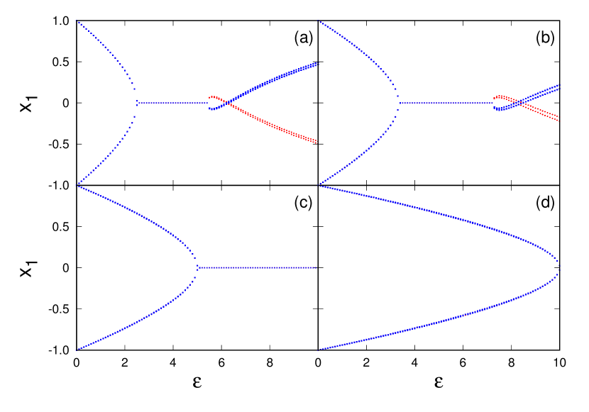
Figure 1: Bifurcation diagram displaying variable $x$ of one of the oscillators, with respect to coupling strength $\varepsilon$. Here the coupling switches between similar and dissimilar variables periodically, with similar-variable coupling (for time $f_{sim}T$) followed by dissimilar-variable coupling (for time $(1-f_{sim})T$), for (a) $f_{sim}$=$0.2$, (b) $f_{sim}$=$0.4$, (c) $f_{sim}$=$0.6$ and (d) $f_{sim}$=$0.8$, and time period of switching $T=0.02$. The two colours represent symmetric solutions around the unstable fixed point, arising from different initial conditions.

Further, notice from Fig. 1a-b that low-amplitude oscillations are restored at higher coupling strengths again, for intermediate $f_{sim}$. Fig. 2 shows the effect of the frequency of switching coupling forms upon the amplitude of the revived oscillations. Increase in frequency of switching leads to the reduction of oscillation amplitude, and the results approach those arising from effective mean-field like dynamical equations (cf. Eqn. V) which will be presented in Section V (namely, Fig. 1(b) approaches Fig. 9(b) obtained from an approximate effective description of the system).

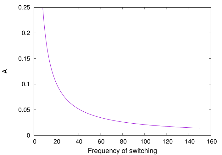
Figure 2: Dependence of $A=x_{max}-x_{min}$ on the frequency of switching (where $x_{max}$/$x_{min}$ are the maximum/minimum values of variable $x$ of an oscillator). Here $f_{sim}=0.4$, $\varepsilon=9.0$, and the coupling switches between similar and dissimilar variables periodically, with similar-variable coupling for time $f_{sim}T$, followed by dissimilar-variable coupling for time $(1-f_{sim})T$, where $1/T$ is the frequency of switching.

III.2 Probabilistic Switching of Coupling Forms

Here the oscillators change their coupling form at intervals of time $T$, with the coupling form chosen probabilistically. We consider the probability for the oscillators to be coupled via similar variables to be $p_{sim}$, and the probability of coupling mediated via dissimilar variables to be $(1-p_{sim})$. For $0<p_{sim}<1$, at the time of switching, the similar-variable coupling form is chosen with probability $p_{sim}$ and the dissimilar-variable form is chosen with probability $(1-p_{sim})$. So larger $p_{sim}$ favours coupling through similar variables and smaller $p_{sim}$ favours dissimilar-variable coupling, with the oscillators always experiencing dissimilar-variable coupling for the limiting case of $p_{sim}=0$ and similar-variable coupling for $p_{sim}=1$. Here the probability $p_{sim}$ plays a role equivalent to $f_{sim}$ in the case of periodic switching of coupling forms.

Fig. 3 shows the bifurcation diagram, with respect to coupling strength, for different $p_{sim}$. Again it is evident that the window of coupling strength over which oscillations are suppressed, depends non-monotonically on $p_{sim}$, as it did under variation of $f_{sim}$ for the case of periodically switched coupling forms (cf. Fig. 4). First, as $p_{sim}$ increases from zero, the fixed point window increases, as seen from Fig. 3a for $p_{sim}=0.2$ vis-a-vis Fig. 3c for $p_{sim}=0.6$. However, when $p_{sim}$ gets even larger this window vanishes entirely, as evident from Fig. 3d, and the oscillations are no longer suppressed anywhere. This suggests that when the probability of coupling through similar variables and dissimilar variables is similar (i.e. $p_{sim}\sim 0.5$) oscillations are suppressed to the greatest degree.

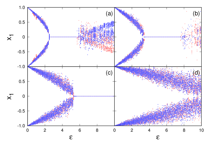
Figure 3: Bifurcation diagram displaying variable $x$ of one of the oscillators, with respect to coupling strength $\varepsilon$. Here the coupling form probabilistically switches at time intervals of $T$ between similar and dissimilar variables, with the probability of similar-variable coupling being $p_{sim}$, and the probability of dissimilar-variable coupling being $(1-p_{sim})$, for (a) $p_{sim}=0.2$, (b) $p_{sim}=0.4$, (c) $p_{sim}=0.6$ and (d) $p_{sim}=0.8$ (with $T=0.02$). The two colours represent emergent dynamics from different initial conditions

Fig. 4 shows the width of fixed point window, with respect to $f_{sim}$ for the case of periodic switching of coupling forms, and $p_{sim}$ for the case of probabilistic switching of coupling forms. As shown, the width of the fixed point window is non-monotonic, and has a maximum at $f_{sim}(p_{sim})\sim 0.58$. Namely, the largest window of fixed point dynamics arises where there is balance in the probability of occurrence of the coupling forms.

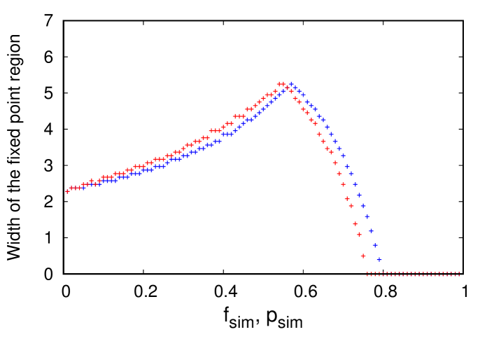
Figure 4: Width of the fixed point window as a function of $f_{sim}$ (blue) for the case of periodic switching of coupling forms, and $p_{sim}$ (red) for the case of probabilistic switching of coupling forms, with switching period $T=0.02$.

IV Global stability measure

The commonly employed linear stability analysis, based on the linearization in the neighbourhood of fixed points, provides only local information about the stability at the fixed point. It cannot accurately indicate the stability for large perturbations, nor the basin of attraction of the dynamics, especially in the presence of other attractors in phase space.

Here we calculate the Basin Stability of the dynamical states basin . This is a more robust and global estimate of stability, and effectively incorporates non-local and non-linear effects on the stability of fixed points. Specifically, Basin Stability is calculated as follows: we choose a large number of random initial conditions, spread uniformly over a volume of phase space, and find what fraction of these are attracted to stable fixed points.

Figs 5 shows the Basin Stability of the fixed point state, in the parameter space of $f_{sim}$ and coupling strengths, for different time periods of switching $T$. Clearly one obtains oscillation suppression in windows of coupling strength and $f_{sim}$, and oscillation revival again beyond the window. The window of coupling strengths that gives rise to fixed points is very sensitive to the frequency of switching, at low frequencies. After a high enough switching frequency (i.e. low enough $T$), the fixed point region remains unchanged, as evident through the fact that Fig. 5a and Fig. 5b are identical.

Now, the dependence of the fixed point window on $f_{sim}$ is actually quite counter-intuitive, as already indicated in the bifurcation diagrams. For rapidly switched coupling forms, at large coupling strengths, the oscillation suppression occurs at an intermediate value of $f_{sim}$. Namely, as the dominance of similar-variable coupling $f_{sim}$ increases the oscillations are first suppressed and then after a point the oscillations are revived again, with the window of fixed points shifting towards higher $f_{sim}$, as coupling strength increases. This is counter-intuitive, as similar-variable coupling is known to only allow oscillations, while dissimilar-variable coupling can yield some windows of oscillation suppression. Also interestingly for low $f_{sim}$, as we increase the coupling strength, first we encounter oscillation suppression and then on further increase of coupling strength the oscillations are restored. So there exists an intermediate window of coupling strength that yields fixed point dynamics.

Fig 6 shows the Basin Stability of the fixed point state, in the parameter space of the frequency of switching and coupling strengths, for different $f_{sim}$. It is clear again that after a critical switching frequency the dynamics does not depend on the rate at which the coupling form is changed. Significantly, it is also evident that fast changes in coupling form, namely lower time period for change, yields large fixed point regions in parameter space. However, at low switching frequencies the emergent dynamics is sensitive to how rapidly the coupling form varies.

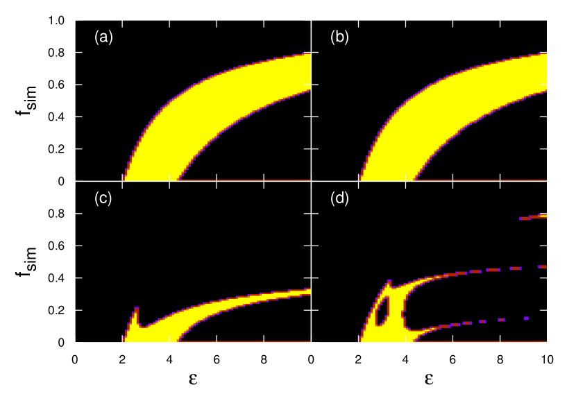
Figure 5: Basin Stability of the fixed point state of coupled oscillators, in the parameter space of coupling strength $\varepsilon$ and $f_{sim}$. Here the coupling periodically switches between similar and dissimilar variables, with similar-variable coupling (for time $f_{sim}T$), followed by dissimilar-variable coupling (for time $(1-f_{sim})T$), for (a) $T=0.01$, (b) $T=0.10$, (c) $T=1.00$ and (d) $T=2.00$. The region in yellow represents fixed point dynamics (i.e. oscillation suppression), and the region in black represents oscillatory dynamics.

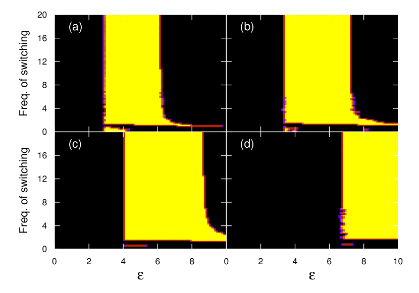
Figure 6: Basin Stability of the fixed point state of coupled oscillators, in the parameter space of coupling strength $\varepsilon$ and frequency of switching. Here the coupling periodically switches between similar and dissimilar variables, with similar-variable coupling (for time $f_{sim}T$), followed by dissimilar-variable coupling (for time $(1-f_{sim})T$), for (a) $f_{sim}=0.3$, (b) $f_{sim}=0.4$, (c) $f_{sim}=0.5$ and (d) $f_{sim}=0.7$. The region in yellow represents fixed point dynamics (i.e. oscillation suppression), and the region in black represents oscillatory dynamics.

Fig 7 shows the Basin Stability of the fixed point state for the case of probabilistically varying coupling form, in the parameter space of $p_{sim}$ and coupling strengths. Interestingly again, as we increase the coupling strength, oscillations first get suppressed and then restored. Also notice the marked similarity of Fig. 7a and Fig. 5a. Namely frequent periodic switching of coupling forms yields the same result as the frequent probabilistic switching of coupling forms.

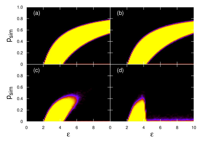
Figure 7: Basin Stability of the fixed point state of coupled oscillators, in the parameter space of coupling strength $\varepsilon$ and $p_{sim}$. Here the coupling probabilistically switches between similar and dissimilar variables, with the probability of similar-variable coupling being $p_{sim}$, and the probability of dissimilar-variable coupling being $(1-p_{sim})$ with the period of switching (a) $T=0.01$, (b) $T=0.02$, (c) $T=0.10$ and (d) $T=1.00$. The region in yellow represents fixed point dynamics (i.e. oscillation suppression), and the region in black represents oscillatory dynamics. Notice the marked similarity of panel (a) with Fig. 5a.

Fig. 8 shows the Basin Stability of the fixed point state, in the parameter space of frequency of switching and coupling strengths. Clearly the effects of the frequency of switching are pronounced over a larger range of switching frequency for probabilistic switching, as compared to periodic switching. But significantly again, it is evident that fast changes in coupling form, namely lower time period for change, yields large fixed point regions in parameter space. Lastly, it is also clear that as the frequency of switching increases, the fixed point region moves towards higher values of $p_{sim}$ where similar-variable coupling dominates. This is again surprising, as similar-variable coupling is known to support only oscillations, while dissimilar-variable coupling has more propensity towards oscillation suppression.

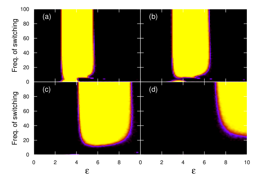
Figure 8: Basin Stability results for coupled oscillators, in the parameter space of coupling strength $\varepsilon$ and frequency of switching, when coupling switches between similar and dissimilar variables probabilistically, with a probability of similar coupling $p_{sim}$, and probability of dissimilar coupling $(1-p_{sim})$, for (a) $p_{sim}=0.2$, (b) $p_{sim}=0.3$, (c) $p_{sim}=0.5$ and (d) $p_{sim}=0.7$. The region in yellow represents fixed point dynamics (i.e. oscillation suppression), and the region in black represents oscillatory dynamics.

V Effective model for time dependent coupling

Now we attempt to rationalize our results through an effective phenomenological model for the dynamics. The idea is to mimic the time-dependent coupling by a coupling form where the similar and dissimilar coupling forms are appropriately weighted by $f_{sim}$. This is given by:

$$\dot{x_{1}} = f^{x}(x_{1},y_{1})+\varepsilon[f_{sim}(x_{2}-x_{1})+(1-f_{sim})(y_{2}-x_{1})]$$

$$\dot{y_{1}} = f^{y}(x_{1},y_{1})$$ (5)

$$\dot{x_{2}} = f^{x}(x_{2},y_{2})+\varepsilon[f_{sim}(x_{1}-x_{2})+(1-f_{sim})(y_{1}-x_{2})]$$

$$\dot{y_{2}} = f^{y}(x_{2},y_{2})$$

This effective picture is expected to hold true when the frequency of switching is very high (namely $T$ is very small). Completely equivalent results can be obtained with $p_{sim}$ in place of $f_{sim}$ in the equations above.

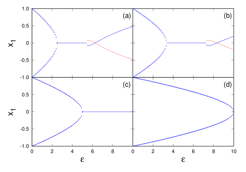
Figure 9: Bifurcation diagram displaying variable $x$ of one of the oscillators of the effective coupled system given by Eqn. V, with respect to coupling strength $\varepsilon$, at different $f_{sim}$ values: (a) $f_{sim}$=$0.2$, (b) $f_{sim}$=$0.4$, (c) $f_{sim}$=$0.6$ and (d) $f_{sim}$=$0.8$. The two colours represent symmetric solutions around the unstable fixed point, arising from different initial conditions.

Fig. 9 displays the bifurcation diagram of the effective coupled system given by Eqn. V, and provides insight into the suppression and revival of oscillations in the coupled oscillator system with time-varying coupling forms. In particular, notice the marked similarity of the fixed point region in Fig. 9 with the fixed point regions evident in Figs. 1 and 3.

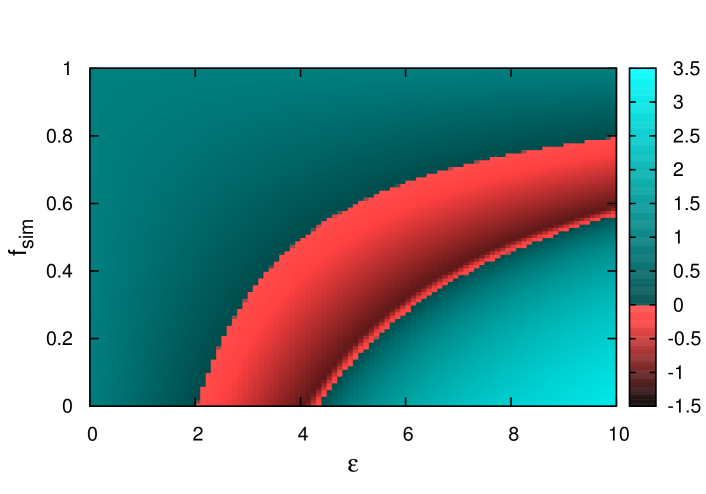
Figure 10: Results from Linear Stability analysis of the effective model of the coupled oscillators given by Eqn. V, in the parameter space of coupling strength $\varepsilon$ and $f_{sim}$. The color code represents the value of the maximum eigen value of the Jacobian corresponding to Eqn. V, $\lambda_{max}$. The region in pink, where $\lambda_{max}<0$, represents stable fixed points. The region in green, where $\lambda_{max}>0$, represents unstable fixed points. Notice the marked similarity with Figs. 5a and 7a.

Increasing the coupling strength, makes the fixed point at zero in Eqn. V unstable, and leads to creation of new fixed points. Fig. 10 shows results from the linear stability analysis of Eqn. V, in the neighbourhood of the fixed point at zero. The region in pink represents the stable fixed point, where the maximum eigen value of the Jacobian corresponding to Eqn. V, $\lambda_{max}$, is negative. The region in green represents unstable fixed points, as $\lambda_{max}>0$ there. Notice the marked similarity of these results with Fig. 5a (or equivalently Fig. 7a), namely the fixed point region is completely well-described by the analysis of Eqn. V when the frequency of switching is high ($\sim 100$ Hz). Significantly then, the results from the global estimates of the basin of stability of the fixed point, for rapid periodic and probabilistic switching of coupling form, are recovered accurately through the linear stability analysis of a set of effective dynamical equations.

VI Conclusions

While the variation in links, namely the connectivity matrix, as a function of time has been investigated in recent times, the dynamical consequences of time-varying coupling forms is still not understood. In this work we have explored this new direction in time-varying interactions, namely we have studied the effect of switched coupling forms on the emergent behaviour. The test-bed of our enquiry is a generic system of coupled Stuart-Landau oscillators, where the form of the coupling between the oscillators switches between the similar and dissimilar (or conjugate) variables. We consider two types of switching, one where the coupling function changes periodically and one where it changes probabilistically. When the oscillators change their coupling form periodically, they are coupled via similar variables for fraction $f_{sim}$ of the cycle, followed by coupling to dissimilar variables for the remaining part. In the case of probabilistic switching, the probability for the oscillators to be coupled via similar variables is $p_{sim}$, and the probability of coupling mediated via dissimilar variables is $(1-p_{sim})$.

We find that time-varying coupling forms suppress oscillations in a window of coupling strengths, with the window increasing with the frequency of switching. That is, more rapid changes in coupling form leads to large windows of oscillation suppression, with the window of amplitude death saturating after a high enough switching frequency. Interestingly, for low $f_{sim}$ ($p_{sim}$), the oscillations are revived again beyond this window. That is, too low or too high coupling strengths yield oscillations, while coupling strengths in-between suppress oscillations.

Also interestingly, the width of the coupling strength window supporting oscillation suppression is non-monotonic with respect to $f_{sim}(p_{sim})$, and has a maximum at $f_{sim}(p_{sim})\sim 0.58$. Namely, the largest window of fixed point dynamics arises where there is balance in the probability of occurrence of the coupling forms.

Focusing on the dependence of the window of oscillation suppression, at fixed coupling strengths and varying predominance of coupling forms, we observe the following: for rapidly switched coupling forms, at large coupling strengths, the oscillation suppression occurs at an intermediate value of $f_{sim}$ ($p_{sim}$). Namely, as the dominance of similar-variable coupling increases the oscillations are first suppressed, and then after a point the oscillations are revived again. The fixed point window shifts towards a higher probability of similar-variable coupling, as coupling strength increases. This is counter-intuitive, as purely similar-variable coupling yields oscillatory behaviour, while dissimilar-variable coupling supports oscillation suppression.

Lastly, we have suggested an effective dynamics that successfully yields the observed behaviour for rapidly switched coupling forms, including an accurate estimate of the fixed point window through stability analysis. Thus our results will potentially enhance the broad understanding of coupled systems with time-varying connections.

References

- (1) Winfree, A.T. ,J. of Theo. Bio., 16, 15-42 (1967)
- (2) Choudhary, A. and Sinha, S., PloS one, 10, p.e0145278 (2015).
- (3) Mondal, A. and Sinha, S. and Kurths, J., Phys. Rev. E, 78, 066209 (2008)
- (4) So, P. and Cotton, Bernard C. and Barreto, E, Chaos, 18, 037114 (2008)
- (5) Tang, J., Scellato, S., Musolesi, M., Mascolo, C. and Latora, V., Phys. Rev. E, 81, 055101, (2010)
- (6) Kohar, V. and Sinha, S., Chaos, Solitons & Fractals, 54 127-134 (2013)
- (7) Masuda, N. and Klemm, K. and Eguíluz, V.M., Phys. Rev. Lett., 111, 188701 (2013)
- (8) Choudhary, A., Kohar, V. and Sinha, S., Sci. Rep., 4, 04308 (2014)
- (9) V. Kohar, Peng Ji, A. Choudhary, S. Sinha, J. Kurths, Phys. Rev. E 90 022812 (2014)
- (10) S. De and S. Sinha, Nonlinear Dynamics 81 (2015) 1741-1749
- (11) N.K. Kamal and S. Sinha, Pramana, 84 (2015) 249-256
- (12) Rungta P. and Sinha S., Europhys. Letts., 112, 60004 (2015)
- (13) Hoppe, K. and Rodgers, G. J., Phys. Rev. E, 88, 042804 (2013)
- (14) Stehlé, J. and Barrat, A. and Bianconi, G., Phys. Rev. E, 81, 035101 (2010)
- (15) F De Vico Fallani, V Latora, L Astolfi, F Cincotti, D Mattia, M G Marciani, S Salinari, A Colosimo and F Babiloni, Journal of Physics A, 41, 224014 (2008)
- (16) Valencia, M. and Martinerie, J. and Dupont, S. and Chavez, M., Phys. Rev. E, 77, 050905 (2008)
- (17) Ahmed, A. and Xing, E.P., PNAS, 106, 11878-11883 (2009).
- (18) M.-Y. Kim, R. Roy, J. L. Aron, T. W. Carr, and I. B. Schwartz, Phys. Rev. Lett., 94, 088101 (2005)
- (19) Cao, Jinde and Chen, Guanrong and Li, Ping, IEEE Transactions on Systems, Man, and Cybernetics, Part B (Cybernetics) , 38, 488-498 (2008).
- (20) Li, Baocheng, Nonlinear Dynamics, 76,1603-1610(2014).
- (21) Sharma, Amit and Shrimali, Manish Dev and Aihara, K., Phys. Rev. E, 90, 062907(2014).
- (22) Karnatak, R., Ramaswamy, R., and Feudel, U., Chaos, Solitons & Fractals, 68, 48-57 (2014).
- (23) Y. Kuramoto, Chemical Oscillations, Waves, and Turbulence, 5-6, Springer (1984)
- (24) Menck, P.J, Heitzig, J., Marwan, N. and Kurths, J, Nature Physics, 9, 89-92 (2013)
- (25) R. Karnatak, R. Ramaswamy and A. Prasad, Phys. Rev. E, 76, 035201 (2007)
- (26) A. Sharma and M. D. Shrimali, Phys. Rev. E, 85, 057204 (2012)
- (27) A. Sharma, M. D. Shrimali and K. Aihara, Phys. Rev. E, 90, 062907 (2014)
- (28) V. Resmi, G. Ambika, R. E. Amritkar and G. Rangarajan, Phys. Rev. E, 85, 046211 (2012)
- (29) G. Saxena , A. Prasad and R. Ramaswamy, Physics Reports, 512, 205-228 (2012)
- (30) V. Resmi, G. Ambika and R. E. Amritkar, Phys. Rev. E, 84, 046212 (2011)
- (31) A. Prasad, Pramana, 81, 407-415 (2013)
- (32) T. Banerjee and D. Ghosh, Phys. Rev. E, 89, 052912 (2014)