NCTS-TH/1702

On New Proposal for Holographic BCFT

Chong-Sun Chu^1,2 Rong-Xin Miao ¹ and Wu-Zhong Guo²

¹Department of Physics, National Tsing-Hua University, Hsinchu 30013, Taiwan

²Physics Division, National Center for Theoretical Sciences, National Tsing-Hua University, Hsinchu 30013, Taiwan

Abstract

This paper is an extended version of our short letter on a new proposal for holographic boundary conformal field, i.e., BCFT. By using the Penrose-Brown-Henneaux (PBH) transformation, we successfully obtain the expected boundary Weyl anomaly. The obtained boundary central charges satisfy naturally a c-like theorem holographically. We then develop an approach of holographic renormalization for BCFT, and reproduce the correct boundary Weyl anomaly. This provides a non-trivial check of our proposal. We also investigate the holographic entanglement entropy of BCFT and find that our proposal gives the expected orthogonal condition that the minimal surface must be normal to the spacetime boundaries if they intersect. This is another support for our proposal. We also find that the entanglement entropy depends on the boundary conditions of BCFT and the distance to the boundary; and that the entanglement wedge behaves a phase transition, which is important for the self-consistency of AdS/BCFT. Finally, we show that the proposal of arXiv:1105.5165 is too restrictive that it always make vanishing some of the boundary central charges.

1 Introduction

BCFT is a conformal field theory defined on a manifold $M$ with a boundary $P$ with suitable boundary conditions. It has important applications in string theory and condensed matter physics near boundary critical behavior [1]. In the spirit of AdS/CFT [2], Takayanagi [3] proposes to extend the $d$ dimensional manifold $M$ to a $d+1$ dimensional asymptotically AdS space $N$ so that $\partial N=M\cup Q$, where $Q$ is a $d$ dimensional manifold which satisfies $\partial Q=\partial M=P$. We mention that the presence of the boundary $Q$ is very natural from the point of view of the UV/IR relation [4] of AdS/CFT correspondence since the presence of boundary in the field theory introduce an IR cutoff and this can be naturally implemented in the bulk with the presence of a boundary. Conformal invariance on $M$ requires that $N$ is part of AdS space. The key point of holographic BCFT is thus to determine the location of boundary $Q$ in the bulk. For interesting developments of BCFT and related topics please see, for example, [5, 6, 7, 8, 9, 10, 11, 12, 13, 14, 15, 16].

The gravitational action for holographic BCFT is given by [3, 5] (taking $16\pi G_{N}=1$)

$$I=\int_{N}\sqrt{G}(R-2\Lambda)+2\int_{Q}\sqrt{h}(K-T)+2\int_{M}\sqrt{g}\ K+2\int_{P}\sqrt{\sigma}\ \theta$$ (1)

where $T$ is a constant and $\theta=\arccos(n_{M}.n_{Q})$ is the supplementary angle between the boundaries $M$ and $Q$, which makes a well-defined variational principle on the corner $P$ [17]. Notice that $T$ can be regarded as the holographic dual of boundary conditions of BCFT since it affects the boundary entropy (and also the boundary central charges, see (55,56) below) which are closely related to the boundary conditions of BCFT [3, 5]. Considering the variation of the on-shell action, we have

$$\delta I = -\int_{Q}\sqrt{h}\left(K^{\alpha\beta}-(K-T)h^{\alpha\beta}\right)\delta h_{\alpha\beta}-\int_{M}\sqrt{g}(K^{ij}-Kh^{ij})\delta g_{ij}+\int_{P}\sqrt{\sigma}\ \theta\sigma^{ab}\delta\sigma_{ab}.$$ (2)

For conformal boundary conditions in CFT, Takayanagi [3] proposes to impose Dirichlet boundary condition on $M$ and $P$, $\delta g_{ij}|_{M}=\delta\sigma_{ab}|_{P}=0$, but Neumann boundary condition on $Q$. And the position of the boundary $Q$ is determined by the Neumann boundary condition

$$K^{\alpha\beta}-(K-T)h^{\alpha\beta}=0.$$ (3)

For more general boundary conditions which break boundary conformal invariance even locally, [3, 5] propose to add matter fields on $Q$ and replace eq.(3) by

$$K_{\alpha\beta}-Kh_{\alpha\beta}=\frac{1}{2}T^{Q}_{\alpha\beta},$$ (4)

where we have included $2Th_{\alpha\beta}$ in the matter stress tensor $T^{Q}_{\alpha\beta}$ on $Q$. For geometrical shape of $M$ with high symmetry such as the case of a disk or half plane, (3) fixes the location of $Q$ and produces many elegant results for BCFT [3, 5, 6]. However since $Q$ is of co-dimension one and its shape is determined by a single embedding function, (3) gives too many constraints and in general there is no solution in a given spacetime such as AdS. On the other hand, of course, one expect to have well-defined BCFT with general boundaries.

To solve this problem, [5] propose to take into account backreactions of $Q$. For 3d BCFT, they show that one can indeed find perturbative solution to (3) if one take into account backreactions to the bulk spacetime. In other words although not all the shapes of boundary $P$ are allowed by (3) in a given spacetime, by carefully tuning the spacetime (which is a solution to Einstein equations) one can always make (3) consistent for any given shape. However, it is still a little restrictive since one has to change both the ambient spacetime and the position of $Q$ for different boundaries of the BCFT.

As motivated in [3, 5], the conditions (3) and (4) are natural from the point of view of braneworld scenario, and so is the backreaction. However from a practical point of view, it is not entirely satisfactory since one has a large freedom to choose the matter fields as long as they satisfy various energy conditions. As a result, it seems one can put the boundary $Q$ at almost any position as one likes. Besides, it is unappealing that the holographic dual depends on the details of matters on another boundary $Q$. Finally, although eq.(4) could have solutions for general shapes by tuning the matters, it is actually too strong since as we will prove in the appendix it always makes vanishing some of the central charges in the boundary Weyl anomaly. In a recent work [18], we propose a new holographic dual of BCFT with $Q$ determined by a new condition (9). This condition is consistent and provides a unified treatment to general shapes of $P$. Besides, as we will show below, it yields the expected boundary contributions to the Weyl anomaly.

Instead of imposing Neumann boundary condition (3), we suggest to impose the mixed boundary conditions on $Q$ [18]:

$$(K^{\alpha\beta}-(K-T)h^{\alpha\beta})\Pi_{+\alpha\beta}^{\ \ \ \alpha^{\prime}\beta^{\prime}}=0,$$ (5)

$$\Pi_{-\alpha\beta}^{\ \ \ \alpha^{\prime}\beta^{\prime}}\delta h_{\alpha^{\prime}\beta^{\prime}}=0.$$ (6)

where $\Pi_{+\alpha\beta}^{\ \ \ \alpha^{\prime}\beta^{\prime}}$ and $\Pi_{-\alpha\beta}^{\ \ \ \alpha^{\prime}\beta^{\prime}}$ are the projection operators satisfying $\Pi_{+\alpha\beta}^{\ \ \ \ \alpha^{\prime}\beta^{\prime}}+\Pi_{-\alpha\beta}^{\ \ \ \ \alpha^{\prime}\beta^{\prime}}=\delta_{\alpha}^{\alpha^{\prime}}\delta_{\beta}^{\beta^{\prime}}$ and $\Pi_{\pm\alpha\beta}^{\ \ \ \ \alpha^{\prime}\beta^{\prime}}\Pi_{\pm\alpha^{\prime}\beta^{\prime}}^{\ \ \ \ \ \alpha_{1}\beta_{1}}=\Pi_{\pm ij}^{\ \ \ \ \alpha_{1}\beta_{1}}$. Since we could impose at most one condition to fix the location of the co-dimension one surface $Q$, we require $\Pi_{+\alpha\beta}^{\ \ \ \alpha^{\prime}\beta^{\prime}}=A_{\alpha\beta}B^{\alpha^{\prime}\beta^{\prime}}$ and $trAB=1$ from $\Pi_{+}\Pi_{+}=\Pi_{+}$. Now the mixed boundary condition (5) becomes

$$(K^{\alpha\beta}-(K-T)h^{\alpha\beta})A_{\alpha\beta}=0,$$ (7)

where $A_{\alpha\beta}$ are non-zero tensors to be determined. It is natural to require that eq. (7) to be linear in $K$ so that it is a second order differential equation for the embedding. Thus we propose the choice $A_{\alpha\beta}=h_{\alpha\beta}$ in [18]. In this paper, we will provide more evidences for this proposal. Besides, we find that the other choices such as

$$A_{\alpha\beta}=\lambda_{1}h_{\alpha\beta}+\lambda_{2}K_{\alpha\beta}+\lambda_{3}R_{\alpha\beta}+\cdots,\;\;\;\lambda_{1},\lambda_{2}\neq 0,\;\;\;$$ (8)

all lead problems.

To sum up, we propose to use the traceless condition

$$T_{BY}{}^{\alpha}_{\ \alpha}=2(1-d)K+2dT=0$$ (9)

to determine the boundary $Q$. Here $T_{\rm BY}{}_{\alpha\beta}=2K_{\alpha\beta}-2(K-T)h_{\alpha\beta}$ is the Brown-York stress tensor on $Q$. In general, it could also depend on the intrinsic curvatures which we will treat in sect.4. A few remarks on (9) are in order. 1. It is worth noting that the junction condition for a thin shell with spacetime on both sides is also given by (4) [17]. However, here $Q$ is the boundary of spacetime and not a thin shell, so there is no need to consider the junction condition. 2. For the same reason, it is expected that $Q$ has no back-reaction on the geometry just as the boundary $M$. 3. Eq. (9) implies that $Q$ is a constant mean curvature surface, which is also of great interests in both mathematics and physics [19] just as the minimal surface. 4. (9) reduces to the proposal by [3] for a disk and half-plane. And it can reproduce all the results in [3, 5, 6]. 5. Eq. (9) is a purely geometric equation and has solutions for arbitrary shapes of boundaries and arbitrary bulk metrics. 6. Very importantly, our proposal gives non-trivial boundary Weyl anomaly, which solves the difficulty met in [3, 5]. In fact as we will show in the appendix the proposal (4) of [3] is too restrictive and always yields $c_{2}=b_{1}=0$ for the central charges in (10,11). Since $b_{1}$ is expected to satisfy a c-like theorem and describes the degree of freedom on the boundary, thus it is important for $b_{1}$ to be non-zero.

Let us recall that in the presence of boundary, Weyl anomaly of CFT generally pick up a boundary contribution $\left<T^{a}_{a}\right>_{P}$ in addition to the usual bulk term $\left<T^{i}_{i}\right>_{M}$, i.e. $\left<T^{i}_{i}\right>=\left<T^{i}_{i}\right>_{M}+\delta(x_{\perp})\left<T^{a}_{a}\right>_{P}$, where $\delta(x_{\perp})$ is a delta function with support on the boundary $P$. Our proposal yields the expected boundary Weyl anomaly for 3d and 4d BCFT [20, 21, 22]:

$$\left<T^{a}_{a}\right>_{P}=c_{1}\mathcal{R}+c_{2}\text{Tr}\bar{k}^{2},\qquad\qquad\qquad\qquad\quad\;\;d=3,$$ (10)

$$\left<T^{a}_{a}\right>_{P}=\frac{a}{16\pi^{2}}E_{4}^{\rm bdy}+b_{1}\text{Tr}\bar{k}^{3}+b_{2}C^{ac}_{\ \ \ bc}\bar{k}_{\ a}^{b},\quad d=4,$$ (11)

where $c_{1},c_{2},b_{1},b_{2}$ are boundary central charges, $a=2\pi^{2}$ is the bulk central charge for 4d CFTs dual to Einstein gravity, $\mathcal{R}$ is intrinsic curvature, $\bar{k}_{ab}$ is the traceless part of extrinsic curvature, $C_{ijkl}$ is the Weyl tensor on $M$ and $(-E_{4}^{\rm bdy})$ is the boundary terms of Euler density $E_{4}$ used to preserve the topological invariance

$$E_{4}^{\rm bdy}=4\left(2\text{Tr}(k\mathcal{R})-k\mathcal{R}+\frac{2}{3}\text{Tr}k^{3}-k\text{Tr}k^{2}+\frac{1}{3}k^{3}\right).$$ (12)

Since $Q$ is not a minimal surface in our case, our results (55,56) are non-trivial generalizations of the Graham-Witten anomaly [23] for the submanifold.

The paper is organized as follows. In sect.2, we study PBH transformations in the presence of submanifold which is not orthogonal to the AdS boundary $M$ and derive the boundary contributions to holographic Weyl anomaly for 3d and 4d BCFT. In sect. 3, we investigate the holographic renormalization for BCFT, and reproduce the correct boundary Weyl anomaly obtained in sect.2, which provides a non-trivial check of our proposal. In sect. 4, we consider the general boundary conditions of BCFT by adding intrinsic curvature terms on the bulk boundary $Q$. In sect.5, we study the holographic entanglement entropy and boundary effects on entanglement. In sect.6, we discuss the phase transition of entanglement wedge, which is important for the self-consistency of AdS/BCFT. Conclusions and discussions are found in sect. 7. The paper is finished with three appendices. In appendix A, we give an independent derivation of the leading and subleading terms of the embedding function by solving directly our proposed boundary condition for $Q$. The result agrees with that obtained in sect.2 using the PBH transformations. In appendix B, we show that the proposal of [3] always make vanish the central charges $c_{2}$ and $b_{1}$ in the boundary Weyl anomaly for 3d and 4d BCFT. In appendix C, we give the details of calculations for the boundary contributions to Weyl anomaly.

Notations: $G_{\mu\nu},\ g_{ij},\ h_{\alpha\beta}$ and $\sigma_{ab}$ are the metrics in $N,\ M,\ Q$ and $P$, respectively. We have $\mu=(1,...,d+1)$, $i=(1,...,d)$, $\alpha=(1,...,d)$ and $a=(1,...,d-1)$. The curvatures are defined by $R^{\rho}_{\ \sigma\mu\nu}=\partial_{\mu}\Gamma^{\rho}_{\sigma\nu}+\Gamma^{\rho}_{\mu\lambda}\Gamma^{\lambda}_{\sigma\nu}-(\mu\leftrightarrow\nu)$, $R_{\mu\nu}=R^{\rho}_{\ \mu\rho\nu}$ and $R=R^{\mu}_{\ \mu}$. The extrinsic curvature on $Q$ are defined by $K=\nabla_{\mu}n^{\mu}$, where $n_{\mu}$ is the unit vector normal to $Q$ and pointing outward from $N$ to $Q$.

Note added: Two weeks after [18], there appears a paper [51] which claims that our calculations of boundary Weyl anomaly (55,56) are not correct. We find they have ignored important contributions from the bulk action $I_{N}$ for 3d BCFT and the boundary action $I_{Q}$ for 4d BCFT. After communication with us, they realize the problems and reproduce our results (55,56) in a new revision of [51]. For the convenience of the reader, we give the details of our calculations in appendix C. We also emphasis here that, from our analysis, it is natural to keep $T$ as a free parameter rather than to set it zero. Otherwise, the corresponding 2d BCFT becomes trivial since the boundary entropy [3] is zero when $T=0$. Besides, we emphasis that, as we previously demonstrated in section 4, by allowing intrinsic curvatures terms on $Q$, one can always make the holographic boundary Weyl anomaly matches the predictions of BCFT with general boundary conditions. This may or may not match with the result of free BCFT since so far it is not clear whether and how non-renormalization theorems hold. However in the special case it holds, e.g. in the presence of supersymmetry, it just means the parameters of the intrinsic curvature terms are fixed, which is completely natural due to the presence of more symmetry.

2 Holographic Boundary Weyl Anomaly

According to [24], the embedding function of the boundary $Q$ is highly constrained by the asymptotic symmetry of AdS, and it can be determined by PBH transformations up to some conformal tensors. By using PBH transformations, we find the leading and subleading terms of the embedding function for $Q$ are universal and can be used to derive the boundary contributions to the Weyl anomaly for 3d and 4d BCFT. It is worth noting that we do not make any assumption about the location of $Q$ in this approach. So the holographic derivations of boundary Weyl anomaly in this section is very strong.

2.1 PBH transformation

Let us firstly briefly review PBH transformation in the presence of a submanifold [24]. Consider a $(p+1)$-dimensional submanifold $\Sigma$ embedded into the $(d+1)$-dimensional bulk $N$ such that it ends on a $p$-dimensional submanifold $\partial\Sigma$ on the $d$-dimensional boundary $M$. Denote the bulk coordinates by $X^{\mu}=(x^{i},\rho)$ and the coordinates on $\Sigma$ by $\tau^{\alpha}=(y^{a},\tau)$ with $i=1,...,d$ and $a=1,...,p$. The embedding function is given by $X^{\mu}=X^{\mu}(\tau^{\alpha})$.

We consider the bulk metric in the FG gauge

$$ds^{2}=\frac{d\rho^{2}}{4\rho^{2}}+\frac{g_{ij}dx^{i}dx^{j}}{\rho}.$$ (13)

Here $\rho=0$ denote the boundary of the metric. It is known that if one assume the metric $g_{ij}$ admits a series expansion in powers of $\rho$, $g_{ij}=\overset{(0)}{g}_{ij}+\rho\overset{(1)}{g}_{ij}+\cdots$, then $\overset{(1)}{g}_{ij}$ can be fixed by the PBH transformation [26]

$$\overset{(1)}{g}_{ij}=-\frac{1}{d-2}\left(R^{(0)}_{ij}-\frac{R^{(0)}}{2(d-1)}g^{(0)}_{ij}\right).$$ (14)

PBH transformations are a special subgroup of diffeomorphism which preserve the FG gauge:

$$\delta\rho=-2\rho\sigma(x),$$ (15)

$$\delta x^{i}=a^{i}=\frac{1}{2}\int_{0}^{\rho}d\rho^{\prime}g^{ij}(x,\rho^{\prime})\partial_{j}\sigma(x)+a^{i}_{0}(x).$$ (16)

Here $\sigma(x)$ is the parameter of Weyl rescalings of the boundary metric, i.e., $\delta_{\sigma}g^{(0)}_{ij}=2\sigma g^{(0)}_{ij}$ and $a^{i}_{0}(x)$ is the diffeomorphism of the boundary $M$. To keep the position of $\partial\Sigma$ on $M$, we require that $a^{i}_{0}(x)|_{\partial\Sigma}=0$.

Next let us include the submanifold. The metric on $\Sigma$ is given by

$$h_{\tau\tau}=\frac{1}{4\tau^{2}}+\frac{1}{\tau}\partial_{\tau}X^{i}\partial_{\tau}X^{j}g_{ij}(X,\tau),$$ (18)

$$h_{ab}=\frac{1}{\tau}\partial_{a}X^{i}\partial_{b}X^{j}g_{ij}(X,\tau).$$

To fix the reparametrization invariance on $\Sigma$, we chose similarly the gauge fixing condition

$$\tau=\rho,\ \ h_{a\tau}=0$$ (19)

Now under a bulk PBH transformation (15,16), one needs to make a compensating diffeomorphism on $\Sigma$ [24] such that $\delta\rho=\delta\tau$ and $\delta h_{a\tau}=\partial_{a}\tilde{\xi}^{\tau}h_{\tau\tau}+\partial_{\tau}\tilde{\xi}^{b}h_{ab}=0$ in order to stay in the gauge (19). This gives

$$\tilde{\xi}^{\tau}=-2\tau\sigma(x)\quad\mbox{and}\quad\tilde{\xi}^{a}=2\int_{0}^{\tau}d\tau^{\prime}\tau^{\prime}h_{\tau\tau}h^{ab}\partial_{b}\sigma.$$ (20)

As a result, $X^{i}$ changes under PBH transformation as

$$\delta X^{i}=\tilde{\xi}^{\alpha}\partial_{\alpha}X^{i}-a^{i},$$ (21)

where $\tilde{\xi}^{\alpha}$ is given by (20) and $a^{i}$ is given by eq.(16). As in the case of the metric, if one expand the embedding function in powers of $\tau$,

$$X^{i}(\tau,y^{a})=\overset{(0)}{X}{}^{i}(y^{a})+\tau\overset{(2)}{X}{}^{i}(y^{a})+\cdots,$$ (22)

the first leading nontrivial term can be fixed by its transformation properties [24]. In fact, since

$$\delta\overset{(0)}{X}{}^{i}=0,$$

$$\delta\overset{(2)}{X}{}^{i}=-2\sigma\overset{(2)}{X}{}^{i}+\frac{1}{2}\overset{(0)}{h}{}^{ab}\partial_{a}\overset{(0)}{X}{}^{i}\partial_{b}\sigma-\frac{1}{2}\overset{(0)}{g}{}^{ij}\partial_{j}\sigma,$$ (23)

one can solve the second equation of (2.1) by

$$\overset{(2)}{X}{}^{i}=\frac{1}{2p}k^{i},$$ (24)

where $k^{i}$ is the trace of the extrinsic curvature of $\partial\Sigma$

$$k^{i}=\overset{(0)}{h}{}^{ab}k^{i}_{ab}=\overset{(0)}{h}{}^{ab}\left(\partial_{a}\partial_{b}\overset{(0)}{X}{}^{i}-\overset{(0)}{\gamma}{}^{c}_{ab}\partial_{c}X^{(0)}{}^{i}+\overset{(0)}{\Gamma}{}^{i}_{jk}\partial_{a}\overset{(0)}{X}{}^{j}\partial_{b}\overset{(0)}{X}{}^{k}\right),$$ (25)

$\overset{(0)}{h}{}^{ab}$ is the inverse of $\overset{(0)}{h}{}_{ab}$ which appears in the expansion:

$$h_{ab}=\frac{1}{\tau}\partial_{a}\overset{(0)}{X}{}^{i}\partial_{b}\overset{(0)}{X}{}^{j}g_{ij}(\overset{(0)}{X},\tau)+\cdots:=\frac{1}{\tau}\overset{(0)}{h}{}_{ab}+\cdots$$ (26)

and $\overset{(0)}{\gamma}{}_{ab}^{c}$ is the Christoffel symbol for the induced metric $\overset{(0)}{h}{}_{ab}$.

Now let us focus on our problem with $p=d-1$, $\Sigma=Q$ and $\partial\Sigma=P$. Inspired by [3], we relax the assumption of [24] and expand $X^{i}$ in powers of $\sqrt{\tau}$ in the presence of a boundary:

$$X^{i}(\tau,y^{a})=\overset{(0)}{X}{}^{i}(y^{a})+\sqrt{\tau}\overset{(1)}{X}{}^{i}(y^{a})+\tau\overset{(2)}{X}{}^{i}(y^{a})+\cdots$$ (27)

This means that $\Sigma=Q$ is not orthogonal to the AdS boundary $M$ generally due to the non-zero $\overset{(1)}{X}{}^{i}(y^{a})$. Then we have

$$h_{\tau a} = \frac{1}{\tau}\partial_{\tau}X^{i}\partial_{a}X^{j}g_{ij}(X,\tau)$$ (28)

$$= \frac{1}{2\tau^{\frac{3}{2}}}\overset{(1)}{X}{}^{i}\partial_{a}\overset{(0)}{X}{}^{j}g^{(0)}_{ij}+\frac{1}{2\tau}\left(2\overset{(2)}{X}{}^{i}\partial_{a}\overset{(0)}{X}{}^{j}\overset{(0)}{g}_{ij}+\overset{(1)}{X}{}^{i}\partial_{a}\overset{(1)}{X}{}^{j}\overset{(0)}{g}_{ij}+\overset{(1)}{X}{}^{i}\partial_{a}\overset{(0)}{X}{}^{j}\overset{(1)}{X}{}^{k}\partial_{k}\overset{(0)}{g}_{ij}\right)+\cdots.\;\;\;\;$$

Imposing the gauge (19), we get

$$\overset{(1)}{X}{}^{i}=|\overset{(1)}{X}|\ n^{i},$$ (29)

$$h^{i}_{j}\overset{(2)}{X}{}^{j}=-\frac{1}{4}h^{ij}\partial_{j}|\overset{(1)}{X}|^{2}-\frac{1}{2}h^{i}_{j}\overset{(0)}{\Gamma}{}^{j}_{kl}n^{k}n^{l}|\overset{(1)}{X}|^{2},$$ (30)

where $n^{i}$ is the normal vector pointing inside from $P$ to $M$, $|\overset{(1)}{X}|=\sqrt{\overset{(1)}{X}{}^{i}\overset{(1)}{X}{}_{i}}$, $h_{ij}:=\overset{(0)}{g}_{ij}-n_{i}n_{j}$ is the zeroth order induced metric on $\Sigma$, $k^{i}=-n^{i}k$ and $k=\nabla_{i}n^{i}$. It is worth noting that $\overset{(2)}{X}{}^{i}$ is on longer a vector due to the appearance of the affine term in eq.(30). This is not surprising since we have imposed the gauge (19) which fixes all the reparametrization of $Q$ except the one acting on $\partial Q=P$ [24]. One can easily check that $\overset{(0)}{\Gamma}{}^{j}_{kl}n^{k}n^{l}$ is indeed covariant under the residual gauge transformations of the reparametrization of $P$. Besides, note that coordinates are not vector generally, so there is no need to require $\overset{(2)}{X}{}^{i}$ to be a vector. What must be covariant are the finial results such Weyl anomaly and entanglement entropy.

Now let us study the transformations of $X^{i}$ under PBH. From eq.(21), we obtain

$$\delta\overset{(0)}{X}{}^{i}=0,$$ (31)

$$\delta\overset{(1)}{X}{}^{i}=-\sigma\overset{(1)}{X}{}^{i},$$ (32)

$$\delta\overset{(2)}{X}{}^{i}=-2\sigma\overset{(2)}{X}{}^{i}+\frac{1}{2}|\overset{(1)}{X}|^{2}h^{ij}\partial_{j}\sigma-\frac{1}{2}(1+2|\overset{(1)}{X}|^{2})n^{i}n^{j}\partial_{j}\sigma.$$ (33)

Using the following formulas

$$\delta_{\sigma}n^{i}=-\sigma n^{i},$$ (34)

$$\delta_{\sigma}k^{i}=-2\sigma k^{i}-p\ n^{i}n^{j}\partial_{j}\sigma,$$ (35)

$$\delta_{\sigma}\overset{(0)}{\Gamma}{}^{i}_{jk}=\delta^{i}_{j}\nabla_{k}\sigma+\delta^{i}_{k}\nabla_{j}\sigma-\overset{(0)}{g}_{jk}\nabla^{i}\sigma,$$ (36)

one can easily check that eqs.(29,30) indeed obey the transformations (32,33). One may also solve (33) directly and obtain for the normal components of $\overset{(2)}{X}{}^{i}$ as:

$$n^{i}n_{j}\overset{(2)}{X}{}^{j}=\frac{1+|\overset{(1)}{X}|^{2}}{2p}k^{i}-\frac{1}{2}|\overset{(1)}{X}|^{2}\overset{(0)}{\Gamma}{}^{n}_{nn}n^{i}+c_{1}(\frac{k^{i}}{p}+\overset{(0)}{\Gamma}{}^{n}_{nn}n^{i}).$$ (37)

Here $\overset{(0)}{\Gamma}{}^{n}_{nn}=\overset{(0)}{\Gamma}{}^{i}_{jk}n_{i}n^{j}n^{k}$ and $c_{1}$ is a parameter to be determined. Note that a term proportional to $n^{i}n^{j}\partial_{j}|\overset{(1)}{X}|^{2}$ from (30) drops out automatically in (37) since $|\overset{(1)}{X}(y^{a})|$ is functions of only the transverse coordinates $y^{a}$, such term vanishes due to the normal derivatives.

As we have mentioned, $\overset{(2)}{X}{}^{i}$ is no longer a vector in the normal sense due to the gauge fixing (19). Instead, $\overset{(2)}{X}{}^{i}$ admit some kinds of deformed covariance under the remaining diffeomorphism after fixing the FG gauge (13) in $N$ and world-volume gauge (19) on $Q$. It is clear that the remaining diffeomorphism are the ones on $M$ and $P$. The key point is that, for every diffeomorphism on $M$, there exists compensating reparametrization on $Q$ in order to stay in the gauge (19). As a result, $\overset{(2)}{X}{}^{i}$ is covariant in a certain sense under the combined diffeomorphisms on $M$ and $Q$. As we will illustrate below, the deformed gauge symmetry is useful and it fixes the value of the parameter $\lambda_{1}$ to be zero.

Without loss of generality, we consider the Gauss normal coordinates $X^{i}=(x,y^{a})$ on $M$

$$ds_{M}^{2}=\overset{(0)}{g}_{ij}dx^{i}dx^{j}=dx^{2}+\left(\sigma_{ab}+2xk_{ij}+x^{2}q_{ij}+\cdots\right)dy^{a}dy^{b},$$ (38)

where $P$ is located at $x=0$, and $Q$ is determined by

$$x=a_{1}(y)\sqrt{\tau}+a_{2}(y)\tau+\cdots$$ (39)

To satisfy the gauge (19), we should choose the coordinates on $Q$ carefully. For example, the natural one $\tau^{\alpha}=(y^{a},\tau)$ does not work. Instead, we should choose $\tau^{\alpha}=(y^{\prime a},\tau)$ with the embedding functions given by

$$\rho=\tau,$$ (40)

$$x=a_{1}(y^{\prime})\sqrt{\tau}+a_{2}(y^{\prime})\tau+\cdots$$ (41)

$$y^{a}=y^{\prime a}-\frac{1}{4}\sigma^{ab}\partial_{b}a_{1}^{2}(y^{\prime})\tau+\cdots$$ (42)

Notice that $n^{i}=(1,0,\cdots,0)$ and $\Gamma^{n}_{nn}=0$ for the Gauss normal coordinates (38). Recall also that $k=-n_{i}k^{i}$, we obtain from eq.(37)

$$a_{2}(y^{\prime})=-\frac{1+a_{1}^{2}(y^{\prime})}{2p}k-c_{1}\frac{k}{p}.$$ (43)

Now let us use the remaining diffeomorphism to fix the parameter $c_{1}$. Consider a remaining diffeomorphism

$$x=x^{\prime}+cx^{\prime 2}+O(x^{\prime 3})$$ (44)

which keeps the position of $P$ and the gauge eqs.(13,19). From eqs.(41,43,44), we have

$$x^{\prime}=x-cx^{2}+O(x^{3})=a_{1}(y^{\prime})\sqrt{\tau}-\left(\frac{1+a_{1}^{2}(y^{\prime})}{2p}k+c_{1}\frac{k}{p}+c\ a_{1}^{2}(y^{\prime})\right)\tau+\cdots$$ (45)

Since the new coordinate $x^{\prime}$ satisfies the gauge (13,19), it must take the form (37) because of PBH transformations. Substituting $n^{\prime i}=(1,0,..,0)$ and $\Gamma^{n^{\prime}}_{n^{\prime}n^{\prime}}=2c$ into eq.(37), we get

$$a^{\prime}_{2}(y^{\prime})=-\frac{1+a_{1}^{2}(y^{\prime})}{2p}k-c_{1}\frac{k}{p}-c\ a_{1}^{2}(y^{\prime})+2cc_{1}$$ (46)

for the new coordinate $x^{\prime}$. Comparing eq.(46) with the coefficients of $\tau$ in eq.(45), we find that they match if and only if $c_{1}=0$. Hence our claim.

As a summary, by using the PBH transformations and the covariance under remaining diffeomorphism, we find the leading and subleading terms of embedding functions are universal and take the following form

$$\overset{(1)}{X}{}^{i}=|\overset{(1)}{X}|\ n^{i},$$ (47)

$$\overset{(2)}{X}{}^{i}=\frac{1+|\overset{(1)}{X}|^{2}}{2p}k^{i}-\frac{1}{4}h^{ij}\partial_{j}|X^{(1)}|^{2}-\frac{1}{2}\overset{(0)}{\Gamma}{}^{i}_{nn}|\overset{(1)}{X}|^{2}$$ (48)

In the Gauss normal coordinates (38), the embedding function has very elegant expression

$$x=a_{1}(y)\sqrt{\tau}-\frac{1+a^{2}_{1}(y)}{2p}k\ \tau+\cdots$$ (49)

These are the main results of this section. One may still doubt eq.(48) due to the non-covariance. Actually, we can derive it from the covariant equation (9) together with the gauge (19). So it must be covariant under the remaining diffeomorphism. This is a non-trivial check of our results. Please see the appendix for the details. Besides, we have checked other choices of boundary conditions such as eq.(7) with $A_{\alpha\beta}=h_{\alpha\beta}+\lambda_{2}K_{\alpha\beta}+\lambda_{3}R_{\alpha\beta}$. They all yield the same results eqs.(47,48,49). This is a strong support for the universality.

2.2 Boundary Weyl anomaly

In this section, we apply the method of [25] to derive the Weyl anomaly (including the boundary contributions to Weyl anomaly [5]) as the logarithmic divergent term of the gravitational action. For our purpose, we focus only on the boundary Weyl anomaly on $P$ below.

Let us quickly recall our main setup. Consider the asymptotically AdS metric

$$ds^{2}=\frac{dz^{2}+g_{ij}dx^{i}dx^{j}}{z^{2}}$$ (50)

where $z=\sqrt{\rho}$, $g_{ij}=g^{(0)}_{ij}+z^{2}g^{(1)}_{ij}+\cdots$, $g^{(0)}_{ij}$ is the metric of BCFT on $M$ and $g^{(1)}_{ij}$, fixed uniquely by the PBH transformation, is given by (14). Without loss of generality, we choose Gauss normal coordinates for the metric on $M$

$$ds_{M}^{2}=g^{(0)}_{ij}dx^{i}dx^{j}=dx^{2}+\left(\sigma_{ab}+2xk_{ij}+x^{2}q_{ab}+x^{3}l_{ab}+\cdots\right)dy^{a}dy^{b},$$ (51)

where the boundary $P$ is located at $x=0$ . The bulk boundary $Q$ is given by $x=X(z,y)$. Expanding it in $z$, we have

$$x=a_{1}z+a_{2}z^{2}+\cdots+(b_{d+1}\ln z+a_{d+1})z^{d+1}+\cdots$$ (52)

where $a_{i}$ and $b_{d+1}$ are functions of $y^{a}$. By using the PBH transformation, we know that $a_{2}$ is universal and can be expressed in terms of $a_{1}$ and the extrinsic curvature $k$ through eq.(49). $a_{1}$ can be determined by the boundary condition on $Q$. Noting that $K^{\alpha}_{\beta}=\frac{a_{1}}{\sqrt{1+a_{1}^{2}}}\delta^{\alpha}_{\beta}+O(z)$, we get the leading term of eq.(7) as

$$\left(K^{\alpha}_{\beta}-(K-T)\delta^{\alpha}_{\beta}\right)A^{\beta}_{\alpha}=\left((1-d)\frac{a_{1}}{\sqrt{1+a_{1}^{2}}}+T\right)A^{\alpha}_{\alpha}+\cdots=0,$$ (53)

where $\cdots$ denotes higher order terms in $z$. It is remarkable that we can solve $a_{1}$ from eq.(53) without any assumption of $A_{ij}$ except its trace is nonzero. In other words, we can solve $a_{1}$ from the universal part of the boundary conditions. From eqs.(49,53), we finally obtain

$$T=(d-1)\tanh\rho_{*},\quad a_{1}=\sinh\rho_{*},\quad a_{2}=-\frac{\text{Tr}k}{2(d-1)}\cosh^{2}\rho_{*},\cdots,$$ (54)

where we have re-parameterized the constant $T$ in terms of $\rho_{*}$, which can be regarded as the holographic dual of boundary conditions for BCFT. That is because, as will be clear soon, $\rho_{*}$ affects the boundary central charges as the boundary conditions do. It should be mentioned that one can also obtain $a_{1},a_{2}$ by directly solving the boundary condition eq.(9) or eq.(7) with $A_{\alpha\beta}=h_{\alpha\beta}+\lambda_{2}K_{\alpha\beta}+\lambda_{3}R_{\alpha\beta}+\cdots$. They yield the same results for $(T,a_{1},a_{2})$ but different results for $(a_{3},a_{4},\cdots)$.

Now we are ready to derive the boundary Weyl anomaly. For simplicity, we focus on the case of 3d BCFT and 4d BCFT. Substituting eqs.(50-54) into the action (1) and selecting the logarithmic divergent terms after the integral along $x$ and $z$, we can obtain the boundary Weyl anomaly. We note that $I_{M}$ and $I_{P}$ do not contribute to the logarithmic divergent term in the action since they have at most singularities in powers of $z^{-1}$ but there is no integration alone $z$, thus there is no way for them to produce $\log z$ terms. We also note that only $a_{2}$ appears in the final results. The terms including $a_{3}$ and $a_{4}$ automatically cancel each other out. This is also the case for the holographic Weyl anomaly and universal terms of entanglement entropy for 4d and 6d CFTs [27, 28]. After some calculations, we obtain the boundary Weyl anomaly for 3d and 4d BCFT as

$$\left<T^{a}_{a}\right>_{P}=\sinh\rho_{*}\ \mathcal{R}-\sinh\rho_{*}\ \text{Tr}\bar{k}^{2},\ \ \ \ \ \ \ \ \ \ \ \ \ \ \ \ \ \ \ \ \ \ \ \ \ \ \ \ \ \ \ \ \ \ \ \text{ for 3d BCFT},$$ (55)

$$\left<T^{a}_{a}\right>_{P}=\frac{1}{8}E_{4}^{\rm bdy}+(\cosh(2\rho_{*})-\frac{1}{3})\text{Tr}\bar{k}^{3}-\cosh(2\rho_{*})C^{ac}_{\ \ \ bc}\bar{k}_{\ a}^{b},\ \text{ for 4d BCFT.}$$ (56)

which takes the expected conformal invariant form [20, 21, 22]. It is remarkable that the coefficient of $E_{4}^{\rm bdy}$ takes the correct value to preserve the topological invariance of $E_{4}$. This is a non-trivial check of our results. Besides, the boundary charges $c_{1},b_{1}$ in (10, 11) are expected to satisfy a c-like theorem [5, 7, 29]. As was shown in [3, 6], null energy condition on $Q$ implies $\rho$ decreases along RG flow. It is also true for us. As a result, eqs.(55, 56) indeed obey the c-theorem for boundary charges. This is also a support for our results. Most importantly, our confidence is based on the above universal derivations, i.e., we do not make any assumption except the universal part of the boundary conditions on $Q$. Last but not least, we notice that our results (55,56) are non-trivial generalizations of the Graham-Witten anomaly [23] for the submanifold, i.e., we find there exists conformal invariant boundary Weyl anomaly for non-minimal surfaces.

We remark that based on the results of free CFTs [21] and the variational principle, it has been suggested that the coefficient of $Ck$ in (56) is universal for all 4d BCFTs [22]. Here we provide evidence, based on holography, against this suggestion: our results agree with the suggestion of [22] for the trivial case $\rho=0$, while disagree generally. As argued in [29], the proposal of [22] is suspicious. It means that there could be no independent boundary central charge related to the Weyl invariant $\sqrt{\sigma}C^{ac}_{\ \ \ bc}\bar{k}_{\ a}^{b}$. However, in general, every Weyl invariant should correspond to an independent central charge, such as the case for 2d, 4d and 6d CFTs. Besides, we notice that the law obeyed by free CFTs usually does not apply to strongly coupled CFTs. See [30, 31, 32, 33] for examples.

To summarize, by using the universal term in the embedding functions eq.(49) and the universal part of the boundary condition eq.(7), we succeed to derive the boundary contributions to Weyl anomaly for 3d and 4d BCFTs. Since we do not need to assume the exact position of $Q$, the holographic derivations of boundary Weyl anomaly here is very strong. On the other hand, since the terms including $a_{3}$ and $a_{4}$ automatically cancel each other out in the above calculations, so far we cannot distinguish our proposal (9) from the other possibilities such as eq.(7) with $A_{\alpha\beta}=h_{\alpha\beta}+\lambda_{2}K_{\alpha\beta}+\lambda_{3}R_{\alpha\beta}$. We will solve this problem in the next section.

3 Holographic Renormalization of BCFT

In this section, we develop the holographic renormalization for BCFT. We find that one should add new kinds of counterterms on boundary $P$ in order to get finite action. Using this scheme, we reproduce the correct boundary Weyl anomaly eqs.(55,56), which provides a strong support for our proposal eq.(9).

3.1 3d BCFT

Let us use the regularized stress tensor [34] to study the boundary Weyl anomaly. This method requires the knowledge of $(a_{3},a_{4},\cdots)$ and thus can help us to distinguish the proposal (9) from the other choices. we will focus on the case of 3d BCFT in this subsection.
The first step is to find a finite action by adding suitable covariant counterterms[34]. We obtain

$$I_{\rm ren} = \int_{N}dx^{4}\sqrt{G}(R-2\Lambda)+2\int_{Q}dx^{3}\sqrt{h}(K-T)+2\int_{M}dx^{3}\sqrt{g}(K-2-\frac{1}{2}R_{M})$$ (57)

$$+2\int_{P}dy^{2}\sqrt{\sigma}(\theta-\theta_{0}-K_{M}),$$

where $I_{M}$ includes the usual counterterms in holographic renormalization [34, 35], $\theta_{0}=\theta(z=0)$ is a constant [5], $K_{M}$ is the Gibbons-Hawking-York term for $R_{M}$ on $M$. Notice that there is no freedom to add other counterterms, except some finite terms which are irrelevant to Weyl anomaly. For example, we may add $\sqrt{\sigma}R_{P}$ and $\sqrt{\sigma}K_{M}^{2}$ to $I_{P}$. However, these terms are invariant under constant Weyl transformations. Thus they do not contribute to the boundary Weyl Anomaly. In conclusion, the regularized action (57) is unique up to some irrelevant finite counterterms.

From the renormalized action, it is straightly to derive the Brown-York stress tensor on $P$

$$B_{ab}=2(K_{Mab}-K_{M}\sigma_{ab})+2(\theta-\theta_{0})\sigma_{ab}$$ (58)

In sprint of [5, 34, 35], the boundary Weyl anomaly is given by

$$\left<T^{a}_{a}\right>_{P}=\lim_{z\to 0}\frac{B^{a}_{a}}{z^{2}}=\lim_{z\to 0}\frac{4(\theta-\theta_{0})-2K_{M}}{z^{2}},$$ (59)

where $\theta=\arccos\frac{x^{\prime}}{\sqrt{g^{xx}+x^{\prime 2}}}+O(z^{3})$, $\theta_{0}=\arccos(\tanh\rho)$ and $K_{M}=z\frac{\partial_{x}(\sqrt{g}\sqrt{g^{xx}})}{\sqrt{g}}+O(z^{3})$. Actually since we are interested only in boundary Weyl anomaly, we do not need to calculate all the components of Brown-York stress tensors on $P$. Instead, we can play a trick. From the constant Weyl transformations $\sigma_{ab}\to e^{2\epsilon}\sigma_{ab}$, $\sqrt{\sigma}\to e^{2\epsilon}\sqrt{\sigma}$, $\theta\to\theta$ and $K_{M}\to e^{-\epsilon}K_{M}$, we can read off the boundary Weyl normally as

$$\int_{P}dy^{2}\sqrt{\sigma_{0}}\left<T^{a}_{a}\right>_{P}=\int_{P}dy^{2}\sqrt{\sigma}\left(4(\theta-\theta_{0})-2K_{M}\right),$$ (60)

which agrees with eq.(59) exactly.

Substituting eqs.(50-54) into eq.(59), we obtain

$$\left<T^{a}_{a}\right>_{P}=-\frac{1}{4}\text{sech}^{2}(\rho)[48a_{3}+\sinh(\rho)\left(2\mathcal{R}+6q-3k^{2}-6\text{Tr}k^{2}\right)+\sinh(3\rho)\left(2q-k^{2}-4\text{Tr}k^{2}\right)]$$ (61)

Comparing eq.(61) with eq.(55), we find that they match if and only if

$$a_{3}=\frac{1}{48}\sinh(\rho)\left(\cosh(2\rho)(-2\mathcal{R}-4q+k^{2}+10\text{Tr}k^{2})-4\mathcal{R}-8q+3k^{2}+12\text{Tr}k^{2}\right),$$ (62)

which is exactly the solution to our proposed boundary condition (9). One can check that eq.(7) with the other choices $A_{\alpha\beta}=h_{\alpha\beta}+\lambda_{2}K_{\alpha\beta}+\lambda_{3}R_{\alpha\beta}$ gives different $a_{3}$ and thus can be ruled out. Following the same approach, we can also derive boundary Weyl anomaly for 4d BCFT, which agrees with eq.(56) if and only if $a_{3}$ and $a_{4}$ are given by the solutions to condition (9). This is a very strong support to the boundary condition (9) we proposed.

To end this section, let us talk more about the stress tensors on $P$. In general, since the Brown-York stress tensor on $Q$ is non-vanishing, we have

$$\delta I_{\rm ren}=\frac{1}{2}\int_{M}\sqrt{g_{0}}T_{M}^{ij}\delta g^{(0)}_{ij}+\frac{1}{2}\int_{P}\sqrt{\sigma_{0}}T^{ab}\delta\sigma_{0ab}+\frac{1}{2}\int_{Q}\sqrt{h}T_{Q}^{\alpha\beta}\delta h_{\alpha\beta}$$ (63)

From the viewpoint of BCFT, the variations of effective action should takes the form

$$\delta I_{\rm eff}=\frac{1}{2}\int_{M}\sqrt{g_{0}}T_{M}^{ij}\delta g^{(0)}_{ij}+\frac{1}{2}\int_{P}\sqrt{\sigma_{0}}\left(T_{e}^{ab}\delta\sigma_{0ab}+J\delta O\right)$$ (64)

where $J$ and $O$ are the currents and operators on $P$, respectively. After the integration along $z$ on $Q$, we can identify $I_{\rm ren}$ with $I_{\rm eff}$. Since $\sigma_{0ab}=\lim_{z\to 0}\frac{h_{ab}}{z^{2}}$, integration of $h_{ab}$ on $Q$ can also contribute to the stress tensor on $P$. So $T_{e}^{ab}$ and $T^{ab}$ are different generally. Interestingly, they always yield the same Weyl anomaly $T_{e}{}^{a}_{\ a}=T^{a}_{\ a}$ due to $T_{Q}{}^{\alpha}_{\ \alpha}=0$ and the fact that the integration on $Q$, i.e. $dzz^{m}$, cannot produce terms of order $O(z^{0})$. An advantage of $T_{e}^{ab}$ is that it is always finite by definition $T_{e}^{ab}=\frac{2}{\sqrt{\sigma_{0}}}\frac{\delta I_{\rm eff}}{\delta\sigma_{0ab}}$, since $I_{\rm eff}$ is finite. The integration of the other components of $h_{\alpha\beta}$ on $Q$ give the new operator $O$ on $P$. It is worth noting that since $h_{\alpha\beta}$ is related to $g_{ij}$ on-shell, the new operator $O$ coming from $h_{\alpha\beta}$ is also related to geometric quantity derived from $g^{(0)}_{ij}$. According to [40], such geometric quantity appears naturally as the new operator on the boundary of BCFT.

3.2 4d BCFT

Now we study the holographic renormalization for 4d BCFT, which is more subtle. We find that one has to add squared extrinsic curvature terms on the corner $P$ in order to make the action finite.
We propose the following renormalized action

$$I_{\rm ren} = \int_{N}dx^{5}\sqrt{G}(R-2\Lambda)+2\int_{Q}dx^{4}\sqrt{h}(K-T)+2\int_{M}dx^{4}\sqrt{g}(K-3-\frac{1}{4}R_{M})$$ (65)

$$+2\int_{P}dy^{3}\sqrt{\sigma}(\theta-\theta_{0}-\frac{1}{2}K_{M}+\alpha R_{P}+\beta\text{Tr}\bar{K}^{2}_{Q}+\gamma).$$

Similar to the case of 3d BCFT, $I_{M}$ includes the usual counterterms in holographic renormalization [34, 35], $\theta_{0}=\theta(z=0)$ is a constant [5] and $K_{M}$ is the Gibbons-Hawking-York term for $R_{M}$ on $M$. It is worth noting that the induced metric on $Q$ is AdS-like, i.e., it can be rewritten into the form of eq.(50) except that now $g_{ij}$ are in powers of $z$ instead of $z^{2}$. In spirit of the holographic renormalization for asymptotically AdS, one can add a constant term $\gamma$ and an intrinsic curvature term $R_{P}$ into $I_{P}$. However, they are not enough to make the action finite. Instead, we have to add the extrinsic curvature terms $\text{Tr}\bar{K}^{2}_{Q}$ on $P$. This maybe due to the presence of the singular corner $P$ and the non-AdS metric on $Q$. Note that $R_{P}\sim\bar{K}^{2}_{Q}\sim O(z^{2})$ are designed to delete the $O(\frac{1}{z})$ divergence in the action . It should be mentioned that $\bar{K}_{Q\ ab}$ can be regarded as new boundary operator from the viewpoints of BCFT, since it is defined by the embedding from $P$ to $Q$ rather than to the spacetime where BCFT lives. On the other hand, $K_{M\ ab}$ is not an independent operator, since it is defined by the derivatives of the metric for BCFT. As a result, if we add $K_{M}^{2}\sim O(z^{2})$ terms on $P$, we get ill-defined stress tensors with $\partial_{x}\delta(x)T_{xa}$, where $x=0$ denotes the location of $P$. This means there is energy flowing outside $P$, which is not a well-defined BCFT. For these reasons, we propose eq.(65) as the renormalized action.

Substituting eqs.(50-54) into the action (65), we can solve $\alpha$, $\beta$ and $\gamma$ that make a finite action. It is remarkable that $a_{3}$ and $a_{4}$ disappear in the divergent terms of the action (65) once we impose the universal relations (54). Thus the solutions to $\alpha$, $\beta$ and $\gamma$ are irrelevant to $a_{3}$ and $a_{4}$. After some calculations, we get

$$\alpha=-\frac{1}{4}\sinh\rho_{*},\ \ \beta=\frac{1}{4}\cosh\rho_{*}\coth\rho_{*},\ \ \gamma=0.$$ (66)

A quick way to derive eq.(66) is to consider $AdS_{5}$ in the bulk and choose spherical coordinates and cylindrical coordinates on $M$ for $\alpha$ and $\beta$, respectively. Note that the new counterterms $\alpha R_{p}\sim\beta\text{Tr}\bar{K}^{2}_{Q}\sim O(\rho_{*})$ vanish for the trivial boundary condition $\rho_{*}=0$.

Now we are ready to calculate the boundary contributions to Weyl anomaly. Similar to the 3d case, from the constant Weyl transformations $\sigma_{ab}\to e^{2\epsilon}\sigma_{ab}$, $\sqrt{\sigma}\to e^{3\epsilon}\sqrt{\sigma}$, $\theta\to\theta$, $K_{M}\to e^{-\epsilon}K_{M}$, $R_{P}\to e^{-2\epsilon}R_{P}$ and $\text{Tr}\bar{K}^{2}_{Q}\to e^{-2\epsilon}\text{Tr}\bar{K}^{2}_{Q}$, we can read off the boundary Weyl anomaly as

$$\int_{P}dy^{3}\sqrt{\sigma_{0}}\left<T^{a}_{a}\right>_{P}=2\int_{P}dy^{3}\sqrt{\sigma}\left((d-1)(\theta-\theta_{0})-K_{M}+(d-3)(\alpha R_{P}+\beta\text{Tr}\bar{K}^{2}_{Q})\right),$$ (67)

To make eq.(67) finite, we solve

$$a_{3}=-\frac{1}{72}\sinh\rho_{*}\left(\cosh(2\rho_{*})\left(\mathcal{R}+4q-k^{2}-9\text{Tr}k^{2}\right)+2\left(\mathcal{R}+4q-k^{2}-6\text{Tr}k^{2}\right)\right),$$ (68)

which is exactly the solution to our proposed boundary condition (9). Substituting the above $a_{3}$ into eq.(67), we get

$$\left<T^{a}_{a}\right>_{P} = \frac{1}{54}\left[-27\text{sech}^{2}(\rho_{*})(48a_{4}+qk-6l-2k\text{Tr}k^{2}-6\text{Tr}k^{3}+\text{Tr}(k\mathcal{R})+7\text{Tr}(kq))\right.$$ (69)

$$-3\cosh(2\rho_{*})\left(k\left(-3\mathcal{R}-12q+k^{2}+27\text{Tr}k^{2}\right)+27l+90\text{Tr}k^{3}-9\text{Tr}(k\mathcal{R})-63\text{Tr}(kq)\right)$$

$$\left.q+9k\mathcal{R}+9kq-81l-13k^{3}+45k\text{Tr}k^{2}-54\text{Tr}(k\mathcal{R})+54\text{Tr}(kq)\ \right]$$

Comparing eq.(70) with eq.(56), we find that they match if and only if

$$a_{4} = \frac{1}{1728}\big{[}24k\mathcal{R}-14k^{3}-21kq+90k\text{Tr}k^{2}+135l+108\text{Tr}k^{3}-90\text{Tr}(k\mathcal{R})-144\text{Tr}(kq)$$ (70)

$$+4\cosh(2\rho_{*})\left(6k\mathcal{R}-4k^{3}+6kq-9\left(3l+6\text{Tr}k^{3}+\text{Tr}(k\mathcal{R})-5\text{Tr}(kq)\right)\ \right)$$

$$+\cosh(4\rho_{*})\left(-2k^{3}+9kq-18k\text{Tr}k^{2}-9\left(3l+12\text{Tr}k^{3}-2\text{Tr}(k\mathcal{R})-8\text{TR}(kq)\right)\ \right)\big{]},$$

which is again the solution to the boundary condition (9) we proposed. The other choices of boundary conditions give different $a_{3}$ and $a_{4}$ and thus can be excluded. In the above calculations, we have used the following formulas

$$E_{4}^{\rm bdy}=4\left(2\text{Tr}(k\mathcal{R})-k\mathcal{R}+\frac{1}{3}k^{3}-k\text{Tr}k^{2}+\frac{2}{3}\text{Tr}k^{3}\right),$$ (71)

$$\text{Tr}\bar{k}^{3}=\frac{2}{9}k^{3}-k\text{Tr}k^{2}+\text{Tr}k^{3},$$ (72)

$$C^{ac}_{\ \ \ bc}\bar{k}_{\ a}^{b}=-\frac{1}{6}k\mathcal{R}-\frac{1}{6}kq+\frac{1}{6}k^{3}-\frac{1}{2}k\text{Tr}k^{2}+\frac{1}{2}\text{Tr}(k\mathcal{R})+\frac{1}{2}\text{Tr}(kq)$$ (73)

in Gauss normal coordinates (51). Since the calculations are quite complicated, the non-patient readers can study some simple examples instead. For example, $AdS$ in spherical coordinates and cylindrical coordinates are good enough to reproduce most of the results above.

To sum up, we have developed a scheme of holographic renormalization for BCFT. We find that it reproduces the correct boundary Weyl anomaly eqs.(55,56) only when $Q$ is determined by eq. (9). This is a non-trivial check of our proposal for holographic BCFT.

4 General Boundary Condition

In this section, we consider more general boundary conditions for BCFT. As we have mentioned before, the constant $T$ in the gravitational action eq.(1) can be regarded as the holographic dual of boundary conditions for BCFT, since it is closely related to boundary central charges. Naturally, we propose to add intrinsic curvature terms on $Q$ to mimic general boundary conditions. For simplicity, we focus on the case of Ricci scalar. Now the gravitational action for holographic BCFT becomes

$$I=\int_{N}\sqrt{G}(R-2\Lambda)+2\int_{Q}\sqrt{h}(K-T-\lambda R_{Q})+2\int_{M}\sqrt{g}\ K+2\int_{P}\sqrt{\sigma}\ \theta,$$ (74)

where $\lambda$ is a constant. Similarly, we suggest to impose the mixed boundary conditions on $Q$ with the non-trivial one given by

$$T_{BY}{}^{\alpha}_{\ \alpha}=2(1-d)K+2dT+2\lambda(d-2)R_{Q}=0.$$ (75)

Below we will apply the methods of sect. 3 and sect. 4 to investigate the boundary contributions to Weyl anomaly. As it is expected, we find the boundary central charges depend on the new parameter $\lambda$. And again, these two methods give the same results only if the bulk boundary $Q$ is determined by the traceless-stress-tensor condition eq.(75).

4.1 General boundary Weyl anomaly I

Now let us use the method of sect.2 to derive the boundary Weyl anomaly. For simplicity, we focus on $AdS_{4}$ with spherical coordinates and cylindrical coordinates below. The generalization to higher dimensions and other metrics is straightforward.

$$ds^{2} = \frac{dz^{2}+dr^{2}+r^{2}d\theta^{2}+r^{2}\sin^{2}\theta d\phi^{2}}{z^{2}},\ \ \text{spherical coordinates}$$ (76)

$$ds^{2} = \frac{dz^{2}+dr^{2}+r^{2}d\theta^{2}+dy^{2}}{z^{2}},\ \ \ \ \ \ \ \ \ \ \ \ \text{cylindrical coordinates}.$$ (77)

$P$ is at $r=r_{0}$ and $Q$ is given by $r=r(z)$ with

$$r=r_{0}+\sinh\rho_{*}z-\frac{k}{4}\cosh^{2}\rho_{*}z^{2}+a_{3}z^{3}+\cdots$$ (78)

where $k$ is $\frac{2}{r_{0}}$ for sphere and $\frac{1}{r_{0}}$ for cylinder. From the leading term of eq.(75), we can re-express $T$ in terms of $\rho_{*}$ and $\lambda$. In general, we get

$$T=(d-1)\tanh\rho_{*}+\lambda(d-1)(d-2)\text{sech}^{2}\rho_{*}.$$ (79)

Substituting eqs.(76-79) into the action (74) and selecting the logarithmic divergent term after the integral along r and z, we can obtain the boundary Weyl anomaly. Similarly, one can check that $I_{M}$ and $I_{P}$ in the action (74) and $a_{3},a_{4}$ in the embedding function (78) are irrelevant in the above derivations. Rewriting the final results into covariant form, we obtain

$$\left<T^{a}_{a}\right>_{P}=\sinh\rho_{*}(1-2\lambda\coth\rho_{*})\ \mathcal{R}-\sinh\rho_{*}(1-2\lambda\tanh\rho_{*})\ \text{Tr}\bar{k}^{2}.$$ (80)

Interestingly, now the central charges with respect to $\mathcal{R}$ and $\text{Tr}\bar{k}^{2}$ become independent, which implies that there are two independent boundary central charges for 3d BCFT generally. This is the expected result, since every independent Weyl invariant should correspond to an independent central charge. The above discussions can be easily generalized to higher dimensions and general metrics. For 4d BCFT, we obtain

$$\left<T^{a}_{a}\right>_{P}=\frac{1}{8}E_{4}^{\rm bdy}+\left(\cosh(2\rho_{*})(1-4\lambda\tanh\rho_{*})-\frac{1}{3}\right)\text{Tr}\bar{k}^{3}-\cosh(2\rho_{*})(1-4\lambda\tanh\rho_{*})C^{ac}_{\ \ \ bc}\bar{k}_{\ a}^{b}$$

Now the central charges related to $\text{Tr}\bar{k}^{3}$ and $C^{ac}_{\ \ \ bc}\bar{k}_{\ a}^{b}$ are still not independent. One can check that, by adding more general curvatures in $I_{Q}$, the boundary central charges can indeed become independent. For example, let us consider the action

$$I=\int_{N}\sqrt{G}(R-2\Lambda)+2\int_{Q}\sqrt{h}(K-T-\lambda R_{Q}-\lambda_{2}\bar{R}_{Q}{}^{\alpha}_{\beta}\bar{R}_{Q}{}^{\beta}_{\gamma}\bar{R}_{Q}{}^{\gamma}_{\alpha})+2\int_{M}\sqrt{g}\ K+2\int_{P}\sqrt{\sigma}\ \theta,$$ (82)

where $\bar{R}_{Q}{}^{\alpha}_{\beta}=R_{Q}{}^{\alpha}_{\beta}+\frac{(d-1)}{\cosh^{2}\rho_{*}}\delta^{\alpha}_{\beta}$. Following the above approach, we derive

$$\left<T^{a}_{a}\right>_{P} = \frac{1}{8}E_{4}^{\rm bdy}+\left(\cosh(2\rho_{*})(1-4\lambda\tanh\rho_{*})-\frac{1}{3}-16\lambda_{2}\tanh^{3}\rho_{*}\text{sech}^{2}\rho_{*}\right)\text{Tr}\bar{k}^{3}$$ (83)

$$-\cosh(2\rho_{*})(1-4\lambda\tanh\rho_{*})C^{ac}_{\ \ \ bc}\bar{k}_{\ a}^{b}$$

We remark that in obtaining the results (4.1) and (83), it is necessary to consider non-AdS solutions in order to derive the central charge related to $C^{ac}_{\ \ \ bc}\bar{k}_{\ a}^{b}$ since $C_{abcd}=0$ for $AdS$.

4.2 General boundary Weyl anomaly II

In this section, we take the method of sect.3 to study the boundary Weyl anomaly for general boundary conditions. Due to the Ricci scalar in $I_{Q}$ (74), we should add new a Gibbons-Hawking-York term $K_{Q}$ in $I_{P}$. Recall that the induced metric on $Q$ is AdS-like, i.e., it can be rewritten into the form of eq.(50) except that now $g_{ij}$ are in powers of $z$ instead of $z^{2}$. In spirit of the holographic renormalization for asymptotically AdS, one can add a constant term and intrinsic curvature terms on $P$. Besides, from the experience of sect.3, one has to add extrinsic curvature terms in order to make the action finite generally. This is may because of the presence of the corner $P$ and the non-AdS metric on $Q$. Based on the above discussions, we propose the following renormalized action for 3d and 4d BCFT

$$I_{re} = \int_{N}dx^{d+1}\sqrt{G}(R-2\Lambda)+2\int_{Q}dx^{d}\sqrt{h}(K-T-\lambda R_{Q})+2\int_{M}dx^{d}\sqrt{g}(K-(d-1)-\frac{1}{2(d-2)}R_{M})$$ (84)

$$+2\int_{P}dy^{d-1}\sqrt{\sigma}(\theta-\theta_{0}-\frac{1}{d-2}K_{M}-2\lambda K_{Q}+\alpha R_{P}+\beta\text{Tr}\bar{K}^{2}_{Q}+\gamma).$$

where $\alpha,\beta,\gamma$ are parameters and will be determined below. For 3d BCFT, we have $\gamma=2\lambda\text{sech}\rho_{*}$, and $\alpha,\gamma$ are free parameters since they are related to finite counterterms. Below, we focus on 4d BCFT.

For simplicity, we focus on $AdS$ with spherical coordinates and cylindrical coordinates.

$$ds^{2} = \frac{dz^{2}+dr^{2}+r^{2}d\Omega^{2}}{z^{2}},\ \ \ \ \ \ \ \ \ \ \ \ \ \ \ \ \ \ \ \ \ \ \ \text{spherical coordinates},$$ (85)

$$ds^{2} = \frac{dz^{2}+dr^{2}+r^{2}d\theta^{2}+\sin^{2}\theta d\phi^{2}+dy_{2}^{2}}{z^{2}},\ \text{cylindrical coordinates I},$$ (86)

$$ds^{2} = \frac{dz^{2}+dr^{2}+r^{2}d\theta^{2}+dy_{1}^{2}+dy_{2}^{2}}{z^{2}},\ \ \ \ \ \ \ \ \text{cylindrical coordinates II},$$ (87)

Again, we put $P$ at $r=r_{0}$ and label $Q$ by $r=r(z)$ with

$$r=r_{0}+\sinh\rho_{*}z-\frac{k}{6}\cosh^{2}\rho_{*}z^{2}+a_{3}z^{3}+a_{4}z^{4}+\cdots$$ (88)

where $k$ take values $(\frac{3}{r_{0}},\frac{2}{r_{0}},\frac{1}{r_{0}})$ for the metrics (85,86,85), respectively. From the traceless-stress-tensor condition eq.(75), we can solve the above embedding function. For the spherical metric (85), we can get exact solution

$$r=\sqrt{r_{0}^{2}\cosh^{2}\rho_{*}-(z-r_{0}\sinh\rho_{*})^{2}}.$$ (89)

For the first kind of cylindrical metric eq.(86), we obtain

$$a_{3} = \frac{\cosh\rho_{*}(9\sinh(2\rho_{*})-4\lambda(9\cosh(2\rho_{*})-8))}{54r_{0}^{2}(1-4\lambda\tanh\rho_{*})},$$ (90)

$$a_{4} = \frac{\cosh\rho_{*}(-84\lambda\sinh\rho_{*}+44\lambda\sinh(3\rho_{*})+\cosh\rho_{*}-11\cosh(3\rho_{*}))}{108r_{0}^{3}(1-4\lambda\tanh\rho_{*})}$$ (91)

As for the second second of cylindrical metric eq.(87), we have

$$a_{3} = \frac{\cosh\rho_{*}(9\sinh(2\rho_{*})-36\lambda\cosh(2\rho_{*})+28\lambda)}{108r_{0}^{2}(1-4\lambda\tanh\rho_{*})},$$ (92)

$$a_{4} = \frac{\cosh\rho_{*}(4\lambda(47\sinh(3\rho_{*})-81\sinh(\rho_{*}))+19\cosh(\rho_{*})-47\cosh(3\rho_{*}))}{864r_{0}^{3}(1-4\lambda\tanh\rho_{*})}$$ (93)

Substituting eqs.(85-88) into the action (84) and requiring the action finite, we derive

$$\alpha=\lambda\cosh\rho_{*}-\frac{\sinh\rho_{*}}{4},\ \ \beta=\frac{1}{4}\cosh\rho_{*}\coth\rho_{*}-\lambda\cosh\rho_{*},\ \ \gamma=4\lambda\ \text{sech}\rho_{*}.$$ (94)

Again, $a_{3}$ and $a_{4}$ do not appear in the divergent terms of the action (84). Actually, we can use only two of the three examples in eqs.(85,86,87) to derive eq.(94). The third one provides a double check of our calculations.

Now we are ready to calculate the boundary contributions to Weyl anomaly. Similar to the cases of sect. 3, with the help of constant Weyl transformations, we can read off the boundary Weyl anomaly as

$$\int_{P}dy^{3}\sqrt{\sigma_{0}}\left<T^{a}_{a}\right>_{P}$$ (95)

$$= 2\int_{P}dy^{3}\sqrt{\sigma}\left(d\,\lambda+(d-1)(\theta-\theta_{0})-K_{M}-2\lambda(d-2)K_{Q}+(d-3)(\alpha R_{P}+\beta\text{Tr}\bar{K}^{2}_{Q})\right),$$

Substituting eqs.(85-94) into the above formula, we can derive the boundary Weyl anomaly for the three examples in eqs.(85,86,87), which exactly agrees with the result eq.(4.1) of last subsection. This is a strong support to our proposal of holographic BCFT with zero trace of the stress tensors on $Q$, i.e., $T_{BY}{}^{\alpha}_{\ \alpha}|_{Q}=0$.

5 Holographic Entanglement Entropy

5.1 General formula

Let us go on to discuss the holographic entanglement entropy. Following [36, 37], it is not difficult to derive the holographic entanglement entropy for a $d$-dimensional BCFT, which is also given by the area of minimal surface

$$S_{A}=\frac{\text{Area}(\gamma_{A})}{4G_{N}},$$ (96)

where $A$ is a $(d-1)$-dimensional subsystem on $M$, and $\gamma_{A}$ denotes the minimal surface which ends on $\partial A$. What is new for BCFT is that the minimal surface could also end on the bulk boundary $Q$, when the subsystem $A$ is close to the boundary $P$. See Fig.1 for example.

We could keep the endpoints of extreme surfaces $\gamma_{A}^{\prime}$ freely on $Q$, and select the one with minimal area as $\gamma_{A}$. It follows that $\gamma_{A}$ is orthogonal to the boundary $Q$ when they intersect

$$n^{a}_{\gamma_{A}}\cdot n_{Q}|_{\gamma_{A}\cap Q}=0.$$ (97)

Here $n_{Q}$ is the normal vector of $Q$ and $n^{a}_{\gamma_{A}}$ are the two independent normal vectors of $\gamma_{A}$. It is easy to see that if $\gamma^{\prime}_{A}$ is not normal to $Q$, one can always deform $\gamma^{\prime}_{A}$ to decrease the area until it is normal to $Q$ . Let us take an example in Fig.1 to illustrate this. For simplicity, we focus on static spacetime and constant time slice. Then the normal vector of $\gamma_{A}$ alone time is orthogonal to $n_{Q}$ trivially. It is worth keeping in mind that the induced metric on constant time slice is Euclidean and positive definite. Below we focus on the case $d=2$. It is straightforward to generalize our discussions to higher dimensions. Consider an extreme surfaces $OA$ in Fig.1, where $O$ is a fixed point in the bulk, and $OA$ is not normal to the boundary $Q$. Then select an arbitrary point $B$ alone $OA$ as long as it is near enough to the boundary. Starting from $B$, we can construct a minimal surface $BA^{\prime}$ that is normal to the boundary and ending on the boundary at $A^{\prime}$ . Since the metric is positive definite and $B$ is near enough to the boundary, we have $BA>BA^{\prime}$ and thus $OBA>OBA^{\prime}$. Next we construct a minimal surface $OA^{\prime}$ linking $A^{\prime}$ and $O$. By definition, it is smaller than $OBA^{\prime}$. As a result, we have $OBA>OBA^{\prime}>OA^{\prime}$. If $OA^{\prime}$ is not orthogonal to $Q$ either, we can repeat the above approach again and again until the extreme surface is normal to $Q$. Now it is clear that the minimal area condition leads to the orthogonal condition (97).

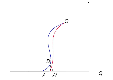
Figure 1: $OBA>OBA^{\prime}>OA^{\prime}$

Another way to obtain the orthogonal condition is that, otherwise there will arise problems in the holographic derivations of entanglement entropy by using the replica trick. In the replica method, one considers the $n$-fold cover $M_{n}$ of $M$ and then extends it to the bulk as $N_{n}$. It is important that $N_{n}$ is a smooth bulk solution. As a result, Einstein equation should be smooth on surface $\gamma_{A}$. Now the metric near $\gamma_{A}$ is given by [37]

$$ds^{2}=\frac{1}{r^{2\varepsilon}}(dr^{2}+r^{2}d\tau^{2})+\left(g_{ij}+2\mathcal{K}_{aij}x^{a}+O(r^{2})\right)dy^{i}dy^{j},$$

where $\varepsilon\equiv 1-\frac{1}{n}$, $r$ is coordinate normal to the surface, $\tau\sim\tau+2\pi n$ is the Euclidean time, $y^{i}$ are coordinates along the surface, $x^{a}=(r\cos\tau,r\sin\tau)$ and $\mathcal{K}_{aij}$ are the two extrinsic curvature tensors. Going to complex coordinates $z=re^{i\tau}$, the $zz$ component of Einstein equations

$$R_{zz}=-\mathcal{K}_{z}\frac{\varepsilon}{z}+\cdots$$ (98)

is divergent unless the trace of extrinsic curvatures vanish $\mathcal{K}_{a}=0$. This gives the condition for a minimal surface [37]. Labeling the boundary $Q$ by $f(z,\bar{z},y)=0$, we obtain the extrinsic curvature of $Q$ as

$$K\sim\varepsilon\ \partial_{z}f\partial_{\bar{z}}f(\frac{\partial_{z}f}{\bar{z}}+\frac{\partial_{\bar{z}}f}{z})+\cdots.$$ (99)

So the boundary condition (9) is smooth only if $\partial_{z}f|_{\gamma_{A}\cap Q}=\partial_{\bar{z}}f|_{\gamma_{A}\cap Q}=0$, which is exactly the orthogonal condition (97). It should be mentioned that the smooth requirement of the general boundary conditions (7) may yield more constraints in addition to the orthogonal condition (97). When $A_{\alpha\beta}$ includes higher curvature terms, sometimes the smooth requirement even leads to contradictions. This can also help us to exclude a large class of $A_{\alpha\beta}$ in the boundary condition (7). Since our boundary condition (9) yields the expected orthogonal condition (97), this is also a support to our proposal.

In summary, the holographic entanglement entropy for BCFT is given by RT formula (96) together with the orthogonal condition (97). As we will show below, there appear many new interesting properties for entanglement due to the presence of boundaries.

5.2 Boundary effects on entanglement

Let us take an simple example to illustrate the boundary effects on entanglement entropy. Consider Poincare metric of $AdS_{3}$

$$ds^{2}=\frac{dz^{2}+dx^{2}-dt^{2}}{z^{2}},$$ (100)

where $P$ is at $x=0$. Solving eq.(9) for $Q$, we get $x=\sinh(\rho)z$ and $T=\tanh\rho\geq 0$. We choose $A$ as an interval with two endpoints at $x=d$ and $x=d+2l$. Due to the presence of boundary, now there are two kinds of minimal surfaces, one ends on $Q$ and the other one does not. It depends on the distance $d$ that which one has smaller area. From eqs.(96,97), we obtain

$$S_{A}=\begin{cases}\frac{1}{2G_{N}}\log(\frac{2l}{\epsilon}),&d\geq d_{c},\\ \frac{\rho}{2G_{N}}+\frac{1}{4G_{N}}\log\Big{(}\frac{4d(d+2l)}{\epsilon^{2}}\Big{)},&d\leq d_{c},\end{cases}$$ (101)

where $d_{c}=l\sqrt{e^{-2\rho}+1}-l$ is the critical distance. The parameter $\rho$ can be regarded as the holographic dual of the boundary condition of BCFT, since it affects the boundary entropy [3] and the boundary central charges (55,56) as the boundary condition does. It is remarkable that entanglement entropy (101) depends on the distance $d$ and boundary condition $\rho$ when it is close enough to the boundary. This is the expected property from the viewpoint of BCFT, where the correlation functions depend on the distance to the boundary [40].

To extract the effects of boundary, let us define a new physical quantity when $A\cap P=0$

$$I_{A}=S^{CFT}_{A}-S^{BCFT}_{A},$$ (102)

where $S^{CFT}_{A}$ is the entanglement entropy when the boundary disappears or is at infinity. For simplicity, we focus on the case $\rho_{*}\geq 0$. In the holographic language, $S^{CFT}_{A}$ is given by the area of minimal surface that does not end on $Q$. Thus, $S^{CFT}_{A}$ is equal to or bigger than $S^{BCFT}_{A}$ and $I_{A}$ is always non-negative. It is expected that boundary does not affect the divergent parts of entanglement entropy when $A\cap P=0$, so all the divergence cancel in eq.(102). As a result, $I_{A}$ is not only non-negative but also finite. For the example discussed above, we have

$$I_{A}=\begin{cases}0,&d\geq d_{c}\\ \frac{1}{4G}\log(\frac{l^{2}}{d(d+2l)})-\frac{\rho}{2G},&0<d<d_{c},\end{cases}$$ (103)

which is indeed both non-negative and finite. Actually in this simple example, $I_{A}$ is just one half of the mutual information between $A$ and its mirror image, so it must be non-negative and finite. See Fig.1. for example. For this simple case, the metric at the mirror image $O^{\prime}$ of a point $O$ is given by the metric at the point $O$. One should keep in mind that the mirror image is only an auxiliary tool, there is no real spacetime outside the boundary $Q$.

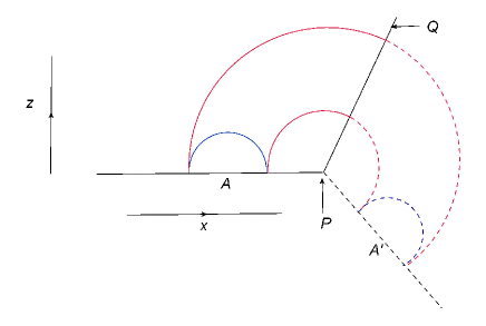
Figure 2: Subsystem $A$ and its mirror image $A^{\prime}$

5.3 Entanglement entropy for stripe

In this subsection, we study the entanglement entropy of stripe in general dimensions. Consider a BCFT defined on $M$ the half space $x\equiv x_{1}<0$, and consider a subsystem $A$ given by the constant time slice $-l<x_{1}<0$, $-L<x_{2},x_{3},\cdots,x_{d-1}<L$. The bulk boundary $Q$ is given by the co-dimension-1 surface $x=z\tan\theta$. Here the parameter $\theta=\arctan(\sinh(\rho_{*}))$, where $\rho_{*}$ is the parameters that we used in previous section. $\theta+\frac{\pi}{2}$ is the angle between $Q$ and $M$. See Fig. 3.

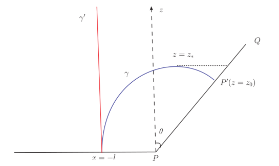
Figure 3: The minimal surface of stripe.

Let the minimal surface $\gamma$ be specified by the equation $x=x(z)$ with the boundary condition

$$x(0)=l.$$ (104)

The induced metric on the minimal surface $\gamma$ is

$$ds^{2}_{\gamma}=\frac{(1+x^{\prime}(z))dz^{2}+\sum_{i=2}^{d-1}dx_{i}^{2}}{z^{2}}.$$ (105)

and gives the equation of motion

$$\frac{x^{\prime}(z)}{z^{d-1}\sqrt{1+x^{\prime}(z)^{2}}}=C,\quad\mbox{$C=$ constant},$$ (106)

for the minimal surface. There are two kinds minimal surface. If $C=0$, the solution is $x=-l$. The other situation is $C\neq 0$, in this case, assume when $z=z_{*}$, $x^{\prime}(z_{*})=\infty$. Let $(x_{0},z_{0})$ be the coordinates of the point $P^{\prime}$ where $Q$ and $\gamma$ intersect. It is $x_{0}\equiv x(z_{0})=z_{0}\tan\theta$. Denote the unit normal vectors of $Q$ by $n^{Q}_{\mu}$, the unit normal vector of $\gamma$ by $n^{\gamma}_{\mu}$. At point $P^{\prime}$ we have $n^{Q}\cdot n^{\gamma}=0$. This gives the boundary condition

$$x^{\prime}(z_{0})=-\cot\theta.$$ (107)

Now we solve (106) together with the boundary conditions (104), (107). Using the condition (107) we have

$$z_{0}^{d-1}=z_{*}^{d-1}\cos\theta,$$ (108)

and

$$x^{\prime}(z)=\frac{(\frac{z}{z_{*}})^{d-1}}{\sqrt{1-(\frac{z}{z_{*}})^{2(d-1)}}}.$$ (109)

We also have the relation

$$x_{0}+l=\int_{0}^{z_{*}}x^{\prime}(z)dz+\int^{z_{*}}_{z_{0}}x^{\prime}(z)dz.$$ (110)

This allow us to solve for $z_{*}$,

$$z_{*}=\frac{l}{F(\theta)},$$ (111)

where

$$F(\theta) = \int_{0}^{1}\frac{x^{d-1}}{\sqrt{1-x^{2(d-1)}}}dx+\int^{1}_{(\cos\theta)^{\frac{1}{d-1}}}\frac{x^{d-1}}{\sqrt{1-x^{2(d-1)}}}dx-\tan\theta(\cos\theta)^{\frac{1}{d-1}}$$ (112)

$$= \frac{B\left(\cos^{2}\theta;\frac{d}{2(d-1)},\frac{1}{2}\right)}{2(d-1)}+2\frac{\sqrt{\pi}\Gamma\left(\frac{d}{2(d-1)}\right)}{\Gamma\left(\frac{1}{2(d-1)}\right)}-\tan\theta(\cos\theta)^{\frac{1}{d-1}},$$

where $B(x;a,b)$ is the incomplete beta function. When $d\geq 3$, there always exist some critical point $\theta_{c}$ such that $F(\theta_{c})=0$, as we can see in the Fig.2 for $d=3$ and $d=4$. One can also show that $\theta_{c}$ is a monotone decreasing function of $d$. In particular in the limit $d\to+\infty$, $\theta_{c}\to 0$.

In the limit $\theta\to\theta_{c}$, $z_{*}\to+\infty$, the solution will tend to the case $C=0$, i.e. the solution $x=-l$. For $\theta>\theta_{c}$ there is only one solution of minimal surface $x=-l$. For $\theta<\theta_{c}$ we have two minimal surface solutions, the desired solution is the one with a smaller area. Consider first the surface $x=-l$. It is easy to obtain its area

$$A_{1}=\frac{A_{0}}{(d-2)\epsilon^{d-2}},$$ (113)

where $A_{0}$ is the area of the entangling surface.

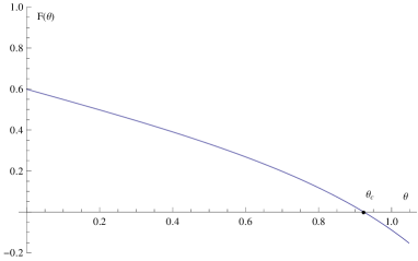
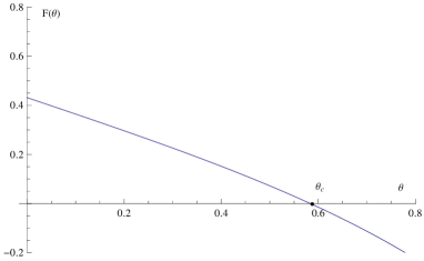
Figure 4: $F(\theta)$ for $d=3$(left) and $d=4$(right)

The area of the other surface is

$$A_{2} = A_{0}(\frac{1}{z_{*}})^{d-2}\Big{(}\int_{\epsilon/z_{*}}^{1}\frac{dx}{x^{d-1}\sqrt{1-x^{2(d-1)}}}+\int^{1}_{(\cos\theta)^{\frac{1}{d-1}}}\frac{dx}{x^{d-1}\sqrt{1-x^{2(d-1)}}}\Big{)}$$

$$= \frac{A_{0}}{(d-2)\epsilon^{d-2}}+\frac{A_{0}}{z_{*}{}^{d-2}}\left(\frac{\sqrt{\pi}\Gamma\big{(}\frac{-(d-2)}{2(d-1)}\big{)}}{(d-1)\Gamma\big{(}\frac{1}{2(d-1)}\big{)}}+\frac{(\cos\theta)^{-\frac{d-2}{d-1}}}{d-2}~{}_{2}F_{1}\Big{(}\frac{1}{2},\frac{-(d-2)}{2(d-1)};\frac{d}{2(d-1)};\cos^{2}\theta\Big{)}\right)+\cdots.$$

(114)

Here $\epsilon$ is the cutoff and ${}_{2}F_{1}(a,b;c;z)$ is the hypergeometric functions. In the limit $\theta\to\theta_{c}$, $z_{*}\to+\infty$, as a result, $A_{2}\to A_{1}$. One could also show $A_{2}$ is a monotone decreasing function of $\theta$ when $\theta<\theta_{c}$. Therefore in the region $\theta<\theta_{c}$, $A_{2}<A_{1}$, the entanglement entropy is given by $\frac{A_{2}}{4G}$.

We remark that our holographic calculation suggests that there is a phase transition at the critical value $\theta=\theta_{c}$. In our example we see that $\theta_{c}$ is independent of the size of the stripe $l$. But it is probably related to the shape of the entangling surface in general. As the parameter $\theta$ is expected to be dual to the boundary condition of BCFT, it is interesting to explore what is the nature of the boundary condition in the field theory that would lead to this phase transition in the BCFT.

6 Entanglement Wedge

According to [38, 39], a sub-region $A$ on the AdS boundary is dual to an entanglement wedge $\mathcal{E}_{A}$ in the bulk where all the bulk operators within $\mathcal{E}_{A}$ can be reconstructed by using only the operators of $A$. The entanglement wedge is defined as the bulk domain of dependence of any achronal bulk surface between the minimal surface $\gamma_{A}$ and the subsystem $A$. Apparently, it seems to conflict with the holographic proposal of BCFT by [3] and us, where the holographic dual of $A$ is given by $N$, which is larger than $\mathcal{E}_{A}$ generally. Of course, there is no contradiction. That is because CFT and BCFT are completely different theories. For CFT, although we do not know the information outside, there still exists spacetime outside $A$. As for BCFT, there is no spacetime outside $A$ at all. Besides, we should impose suitable boundary conditions for BCFT, while there is no need to set boundary condition on the entangling surface for CFT.

It is interesting to study the entanglement wedge in the framework of AdS/BCFT. For simplicity, we focus on the static spacetime and constant time slice. Recall that the entanglement wedge is given by the region between the minimal surface $\gamma_{A}$ and the subsystem $A$ on $M$. A key observation is that entanglement wedge behaves a phase transition and becomes much larger than that within AdS/CFT, when $A$ is increasing and approaching to the boundary. See Fig.3 for example. This phase transition is important for the self-consistency of holographic BCFT. If there is no phase transition, then the entanglement wedge is always given by the first kind (left hand side of Fig.3). When $A$ fills with the whole boundary $M$ and $P$, there are still large space left outside the entanglement wedge, which means there are operators in the bulk cannot be reconstructed by all the operators on the boundary. Thanks to the phase transition, the entanglement wedge for large A is given by the second kind ( right hand side of Fig.3). As a result all the bulk operators can be reconstructed by using the operators on the boundary.

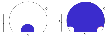
Figure 5: Entanglement wedge for small $A$ and large $A$

7 Conclusions and Discussions

In this letter, we have proposed a new holographic dual of BCFT, which can accommodate all possible shapes of the boundary $P$ with a unified prescription. The key idea is to impose the mixed boundary condition (9) so that there is only one constraint for the co-dimension one boundary $Q$. In general there could be more than one self-consistent boundary conditions for a theory [41], so the proposals of [3] and ours have no contradiction in principle. However, the proposal of [3] is too restrictive to include the general BCFT. The main advantage of our proposal is that we can deal with all shapes of the boundary $P$ easily and that it can accommodate nontrivial boundary Weyl anomaly as is needed in a general BCFT. It is appealing that the bulk boundary $Q$ is given by a constant mean curvature surface, which is a natural generalization of the minimal surface.

Applying the new AdS/BCFT, we obtain the expected boundary Weyl anomaly for 3d and 4d BCFT and the obtained boundary central charges satisfy naturally a c-like theorem holographically. As a by-product, we give a holographic disproof of the proposal [22] and clarify that the validity of the $S_{RE}=S_{EE}$ conjecture [42] which is based on [22] and is sensitively dependent on the choices of boundary conditions of non-free BCFT. Besides, we find the holographic entanglement entropy is given by the RT formula together with the condition that the minimal surface must be orthogonal to $Q$ if they intersect. The presence of boundaries lead to many interesting effects, e.g. phase transition of the entanglement wedge. Of course, many things are left to be explored, for instance, the holographic Rényi entropy [43, 44], the edge modes [45, 46], the shape dependence of entanglement [47, 48], the applications to condensed matter and the relation between BCFT and quantum information [49]. Finally, it is straightforward to generalize our work to Lovelock gravity, higher dimensions and general boundary conditions.

Appendix A Another Derivation of (48)

In sect. 2.1, we have obtained the key result (48) from the PBH transformation together with the explicit requirement of covariance under the residual diffeomorphism of the gauge fixing condition (19). In this appendix, we derive eq.(48) directly from the covariant equation (9) and the gauge fixing (19). The analysis is manifestly covariant with respect to (19) and provides an independent derivation of the (48).

To compute $K$, we note that the extrinsic curvature $K_{\alpha\beta}$ on $Q$ is

$$K_{\alpha\beta}=n^{Q}_{\mu}K^{\mu}_{\alpha\beta},$$ (115)

where

$$K^{\mu}_{\alpha\beta}=\partial_{\alpha}\partial_{\beta}X^{\mu}-\gamma_{\alpha\beta}^{\delta}\partial_{\delta}X^{\mu}+\Gamma_{\nu\lambda}^{\mu}\partial_{\alpha}X^{\lambda}\partial_{\beta}X^{\nu},$$ (116)

$\gamma_{\alpha\beta}^{\delta}$ is the Christoffel symbol for the induced metric $h_{\alpha\beta}$ and $n^{Q}_{\mu}$ is the unit normal vector on $Q$. The components of $K^{\mu}_{\alpha\beta}$ can be worked out easily. Expanded in powers of $\sqrt{\tau}$ for small $\tau$, we have

$$K^{\rho}_{\tau\tau}=\frac{({\overset{\text{\tiny{(1)}}}{X}{}^{i}})^{2}}{2\tau}-\frac{1}{\sqrt{\tau}}\frac{{\overset{\text{\tiny{(1)}}}{X}{}^{i}}{\overset{\text{\tiny{(2)}}}{X}{}_{i}}+\frac{1}{2}{\overset{\text{\tiny{(0)}}}{\Gamma}{}^{m}_{ki}\ \overset{\text{\tiny{(1)}}}{X}{}^{i}\overset{\text{\tiny{(1)}}}{X}{}^{k}\overset{\text{\tiny{(1)}}}{X}{}_{m}}}{1+({\overset{\text{\tiny{(1)}}}{X}{}^{i}})^{2}}+\frac{2}{\sqrt{\tau}}{\overset{\text{\tiny{(1)}}}{X}{}^{i}}{\overset{\text{\tiny{(2)}}}{X}{}_{i}}+\frac{1}{\sqrt{\tau}}{\overset{\text{\tiny{(0)}}}{\Gamma}{}^{m}_{ki}\ \overset{\text{\tiny{(1)}}}{X}{}^{i}\overset{\text{\tiny{(1)}}}{X}{}^{k}\overset{\text{\tiny{(1)}}}{X}{}_{m}}+O(1),$$ (117)

$$K^{\rho}_{ab}=\frac{2({\overset{\text{\tiny{(1)}}}{X}{}^{i}})^{2}\overset{(0)}{h}_{ab}}{1+({\overset{\text{\tiny{(1)}}}{X}{}^{i}})^{2}}+\sqrt{\tau}\frac{2{\overset{\text{\tiny{(1)}}}{X}{}_{i}}k^{i}_{ab}}{1+({\overset{\text{\tiny{(1)}}}{X}{}^{i}})^{2}}+8\sqrt{\tau}\frac{{\overset{\text{\tiny{(1)}}}{X}{}^{i}}{\overset{\text{\tiny{(2)}}}{X}{}_{i}}+\frac{1}{2}{\overset{\text{\tiny{(0)}}}{\Gamma}{}^{m}_{ki}\ \overset{\text{\tiny{(1)}}}{X}{}^{i}\overset{\text{\tiny{(1)}}}{X}{}^{k}\overset{\text{\tiny{(1)}}}{X}{}_{m}}}{(1+({\overset{\text{\tiny{(1)}}}{X}{}^{i}})^{2})^{2}}-4\sqrt{\tau}{\overset{\text{\tiny{(1)}}}{X}{}_{i}}k^{i}_{ab}+O(\tau),\;\;\;\;\;\;$$ (118)

$$K^{i}_{\tau\tau}=-\frac{{\overset{\text{\tiny{(1)}}}{X}{}^{i}}}{4\tau^{3/2}}-\frac{1}{2\tau}\frac{{\overset{\text{\tiny{(1)}}}{X}{}^{i}}{\overset{\text{\tiny{(2)}}}{X}{}_{i}}+\frac{1}{2}{\overset{\text{\tiny{(0)}}}{\Gamma}{}^{m}_{ki}\ \overset{\text{\tiny{(1)}}}{X}{}^{i}\overset{\text{\tiny{(1)}}}{X}{}^{k}\overset{\text{\tiny{(1)}}}{X}{}_{m}}}{1+({\overset{\text{\tiny{(1)}}}{X}{}^{i}})^{2}}{\overset{\text{\tiny{(1)}}}{X}{}^{i}}+\frac{1}{4\tau}\overset{\text{\tiny{(0)}}}{\Gamma}{}^{i}_{km}\ \overset{\text{\tiny{(1)}}}{X}{}^{k}\overset{\text{\tiny{(1)}}}{X}{}^{m}+O(\frac{1}{\tau^{1/2}}),$$ (119)

$$K^{i}_{ab}=-\frac{1}{\sqrt{\tau}}\frac{\overset{(0)}{h}_{ab}}{1+({\overset{\text{\tiny{(1)}}}{X}{}^{i}})^{2}}{\overset{\text{\tiny{(1)}}}{X}{}^{i}}+k^{i}_{ab}-\frac{2}{1+({\overset{\text{\tiny{(1)}}}{X}{}^{i}})^{2}}\overset{(0)}{h}_{ab}\overset{\text{\tiny{(2)}}}{X}{}^{i}+\frac{{\overset{\text{\tiny{(1)}}}{X}{}_{i}}k^{i}_{ab}{\overset{\text{\tiny{(1)}}}{X}{}^{i}}}{1+({\overset{\text{\tiny{(1)}}}{X}{}^{i}})^{2}}$$

$$\qquad\qquad\qquad\qquad\qquad\qquad\qquad\qquad\qquad+4\frac{{\overset{\text{\tiny{(1)}}}{X}{}^{i}}{\overset{\text{\tiny{(2)}}}{X}{}_{i}}+\frac{1}{2}{\overset{\text{\tiny{(0)}}}{\Gamma}{}^{m}_{ki}\ \overset{\text{\tiny{(1)}}}{X}{}^{i}\overset{\text{\tiny{(1)}}}{X}{}^{k}\overset{\text{\tiny{(1)}}}{X}{}_{m}}}{(1+({\overset{\text{\tiny{(1)}}}{X}{}^{i}})^{2})^{2}}{\overset{\text{\tiny{(1)}}}{X}{}^{i}}+O(\tau^{1/2}),$$ (120)

Since $n^{Q}_{\mu}\frac{\partial X^{\mu}}{\partial\tau}=0$, we have

$$n^{Q}_{\rho}=-n^{Q}_{i}\frac{\partial X^{i}}{\partial\tau}.$$ (121)

The trace $K$ is

$$K=-(p+1)\sqrt{\tau}n^{Q}_{i}{\overset{\text{\tiny{(1)}}}{X}{}^{i}}-2\tau\frac{(p+1)({\overset{\text{\tiny{(1)}}}{X}{}^{i}})^{2}+p}{1+({\overset{\text{\tiny{(1)}}}{X}{}^{i}})^{2}}n^{Q}_{j}\overset{\text{\tiny{(2)}}}{X}{}^{j}+\tau n^{Q}_{i}k^{i}+\tau\frac{n^{Q}_{i}\overset{\text{\tiny{(0)}}}{\Gamma}{}^{i}_{km}\ \overset{\text{\tiny{(1)}}}{X}{}^{k}\overset{\text{\tiny{(1)}}}{X}{}^{m}}{1+({\overset{\text{\tiny{(1)}}}{X}{}^{i}})^{2}}+\cdots.$$ (122)

Generally $n_{\rho}$ and $n_{i}$ can be expanded as

$$n^{Q}_{\rho}=\frac{1}{\sqrt{\tau}}\overset{\text{\tiny{(0)}}}{n}{}^{Q}_{\rho}+\overset{\text{\tiny{(1)}}}{n}{}^{Q}_{\rho}+\cdots,\quad n^{Q}_{i}=\frac{1}{\sqrt{\tau}}\overset{\text{\tiny{(0)}}}{n}{}^{Q}_{i}+\overset{\text{\tiny{(1)}}}{n}{}^{Q}_{i}+\cdots.$$ (123)

Taking them to (121) we have

$$\overset{\text{\tiny{(0)}}}{n}{}^{Q}_{\rho}=-\frac{1}{2}\overset{\text{\tiny{(0)}}}{n}{}^{Q}_{i}{\overset{\text{\tiny{(1)}}}{X}{}^{i}},$$ (124)

$$\overset{\text{\tiny{(1)}}}{n}{}^{Q}_{\rho}=-\frac{1}{2}\overset{\text{\tiny{(1)}}}{n}{}^{Q}_{i}{\overset{\text{\tiny{(1)}}}{X}{}^{i}}-\overset{\text{\tiny{(0)}}}{n}{}^{Q}_{i}\overset{\text{\tiny{(2)}}}{X}{}^{i}.$$ (125)

Using the relation

$$h_{\alpha\beta}=\frac{\partial X^{\mu}}{\partial x^{\alpha}}\frac{\partial X^{\nu}}{\partial x^{\beta}}\tilde{h}_{\mu\nu},$$ (126)

where $ds_{Q}^{2}=h_{\alpha\beta}d\tau^{\alpha}d\tau^{\beta}=\tilde{h}_{\mu\nu}dX^{\mu}dX^{\nu}$ is the induced metric on $Q$, we obtain that also $\tilde{h}_{\rho i}=0$. Hence

$$h^{\tau\tau}=\tilde{h}^{\rho\rho}=G^{\rho\rho}-(n^{Q}_{\rho})^{2}G^{\rho\rho}$$ (127)

and as a result

$$\overset{\text{\tiny{(0)}}}{n}{}^{Q}_{i}{\overset{\text{\tiny{(1)}}}{X}{}^{i}}=-\frac{\sqrt{({\overset{\text{\tiny{(1)}}}{X}{}^{i}})^{2}}}{\sqrt{1+({\overset{\text{\tiny{(1)}}}{X}{}^{i}})^{2}}},$$ (128)

$$\overset{\text{\tiny{(1)}}}{n}{}^{Q}_{i}{\overset{\text{\tiny{(1)}}}{X}{}^{i}}=-2\overset{\text{\tiny{(0)}}}{n}{}^{Q}_{i}\overset{\text{\tiny{(2)}}}{X}{}^{i}-2\frac{{\overset{\text{\tiny{(1)}}}{X}{}^{i}}{\overset{\text{\tiny{(2)}}}{X}{}_{i}}+\frac{1}{2}{\overset{\text{\tiny{(0)}}}{\Gamma}{}^{m}_{ki}\ \overset{\text{\tiny{(1)}}}{X}{}^{i}\overset{\text{\tiny{(1)}}}{X}{}^{k}\overset{\text{\tiny{(1)}}}{X}{}_{m}}}{\sqrt{({\overset{\text{\tiny{(1)}}}{X}{}^{i}})^{2}}(1+({\overset{\text{\tiny{(1)}}}{X}{}^{i}})^{2})^{3/2}}.$$ (129)

The gauge $h_{a\tau}=0$ lead to the result $\partial_{a}\overset{\text{\tiny{(0)}}}{X}_{i}{\overset{\text{\tiny{(1)}}}{X}{}^{i}}=0$, which means ${\overset{\text{\tiny{(1)}}}{X}{}^{i}}$ is orthogonal to boundary submanifold $P$. Using $n^{Q}_{\mu}\partial_{a}X^{\mu}=0$ one could show that $\overset{\text{\tiny{(0)}}}{n}{}^{Q}_{i}$ is also orthogonal to $P$. We have the following relations

$${\overset{\text{\tiny{(1)}}}{X}{}^{i}}=\sqrt{({\overset{\text{\tiny{(1)}}}{X}{}^{i}})^{2}}n^{i},$$ (130)

$$\overset{\text{\tiny{(0)}}}{n}{}^{Q}_{i}=-\frac{1}{\sqrt{1+({\overset{\text{\tiny{(1)}}}{X}{}^{i}})^{2}}}n_{i},$$

where $n_{i}$ is the unit normal vector of $P$. Taking (123)(128)(130) into (122) we have

$$K=-(p+1)\overset{\text{\tiny{(0)}}}{n}{}^{Q}_{i}{\overset{\text{\tiny{(1)}}}{X}{}^{i}}+\sqrt{\tau}\overset{\text{\tiny{(0)}}}{n}{}^{Q}_{i}k^{i}-\sqrt{\tau}\frac{2p}{1+({\overset{\text{\tiny{(1)}}}{X}{}^{i}})^{2}}\overset{\text{\tiny{(0)}}}{n}{}^{Q}_{i}\overset{\text{\tiny{(2)}}}{X}{}^{i}+p\sqrt{\tau}\frac{{\overset{\text{\tiny{(0)}}}{\Gamma}{}^{m}_{ki}\ \overset{\text{\tiny{(1)}}}{X}{}^{i}\overset{\text{\tiny{(1)}}}{X}{}^{k}\overset{\text{\tiny{(1)}}}{X}{}_{m}}}{(1+({\overset{\text{\tiny{(1)}}}{X}{}^{i}})^{2})^{3/2}\sqrt{({\overset{\text{\tiny{(1)}}}{X}{}^{i}})^{2}}}+O(\tau).$$ (131)

Now on the surface $Q$, $K=\frac{p+1}{p}T$, we obtain

$$n_{i}{\overset{\text{\tiny{(1)}}}{X}{}^{i}}=\sqrt{\frac{T^{2}}{p^{2}-T^{2}}},$$ (132)

$$n_{i}\overset{\text{\tiny{(2)}}}{X}{}^{i}=\frac{1+({\overset{\text{\tiny{(1)}}}{X}{}^{i}})^{2}}{2p}n_{i}k^{i}-\frac{1}{2}n_{i}\overset{\text{\tiny{(0)}}}{\Gamma}{}^{i}_{km}\overset{\text{\tiny{(1)}}}{X}{}^{k}\overset{\text{\tiny{(1)}}}{X}{}^{m}.$$ (133)

Recall that from the gauge $h_{\tau a}=0$, we can solve the transverse components of $X^{i}$ as eqs.(29,30). Combining eqs.(132,133) and eqs.(29,30) together, we recover exactly eqs.(47,48).

Appendix B Boundary Weyl Anomaly for the Proposal of [3]

In this appendix, we show that the BC (4) proposed by [3] always make vanish the central charges $c_{2}$ and $b_{1}$ in the boundary Weyl anomaly (10,11) for 3d and 4d BCFT. Since $b_{1}$ is expected to satisfy a c-like theorem and describes the degree of freedom on the boundary, thus it is important for $b_{1}$ to be non-zero. We emphasis that this holds for any energy-momentum tensor $T^{Q}_{\alpha\beta}$ on $Q$ as long as the BC (4) holds. In this sense, the proposal of [3] is too restrictive to include the general BCFT, in particular, the non-trivial 4d BCFT.

Let us first start with a simple example to see explicitly how $c_{2}$ and $b_{1}$ vanish in the proposal of [3]. Consider $AdS$ with cylindrical coordinates on $M$ eqs.(77,87) so that only the $\text{Tr}\bar{k}^{d-1}$ terms are non-vanishing in the Weyl anomaly (10,11). We note that in the present case, the equation (4) does not admit a solution with a constant $T$ term and one needs to include on $Q$ either nontrivial matter fields or higher derivatives gravitational action terms. For simplicity, let us consider the addition of an intrinsic Ricci scalar $R_{Q}$ on $Q$. In other words, we focus on the action (74). Requiring all the components of stress tensors on $Q$ vanishing, we get the following exact solutions

$$\lambda=\frac{1}{2(d-2)}\coth\rho_{*},\ \ T=(d-1)\coth(2\rho_{*}),\ \ r=r_{0}+\sinh\rho_{*}\ z.$$ (134)

Substituting eqs.(77,87,134) into the action (74) and selecting the logarithmic divergent term after integration alone $r$ and $z$, we find

$$\left<T^{a}_{a}\right>_{P}=0$$ (135)

for both 3d and 4d BCFT. This means that $c_{2}=b_{1}=0$. This example can be easily generalized to include general higher curvature terms, i.e., we replace $R_{Q}$ by $L(R_{Q\alpha\beta\lambda\gamma})$ in action (74). Using the trick of [27], we expand $L(R_{Q\alpha\beta\lambda\gamma})$ around a ‘background-curvature’ $\bar{R}_{Q\alpha\beta\lambda\gamma}=-\frac{1}{\cosh^{2}\rho_{*}}(h_{\alpha\lambda}h_{\beta\gamma}-h_{\alpha\gamma}h_{\beta\lambda})$. Then we find only the first a few terms up to $(R_{Q}-\bar{R}_{Q})^{d-1}\sim z^{d-1}$ contribute to the boundary Weyl anomaly for $d$-dimensional BCFT. We have worked out the cases for 3d and 4d BCFT on cylinders and find they all yield eq.(135). So the boundary Weyl anomaly $c_{2},b_{1}$ indeed vanish for 3d and 4d BCFT in the proposal of [3]. We have also constructed a model with only matter on $Q$ (non-minimally coupled scalar field with suitable potential energy), which also yield $c_{2}=b_{1}=0$.

Now let us present the general proof. Consider the following action

$$I=\int_{N}\sqrt{G}(R-2\Lambda)+2\int_{Q}\sqrt{h}\left(K-T+L_{m}(\phi)\right)+2\int_{M}\sqrt{g}\ K+2\int_{P}\sqrt{\sigma}\ \theta$$ (136)

where $L_{m}(\phi)$ is the Lagrangian of matter fields $\phi$ on $Q$. According to [25], we can derive the Weyl anomaly as the logarithmic divergent term of the gravitational action. Recall that $I_{M}$ and $I_{P}$ do not contribute the logarithmic divergent term . Considering the variation of the on-shell action, we have

$$\delta I = -\int_{Q}\sqrt{h}\left((K^{\alpha\beta}-(K-T)h^{\alpha\beta}-\frac{1}{2}T^{Q}_{\alpha\beta})\delta h_{\alpha\beta}+E_{\phi}\delta\phi\right)$$ (137)

$$\qquad\qquad-\int_{M}\sqrt{g}(K^{ij}-Kh^{ij})\delta g_{ij}+\int_{P}\sqrt{\sigma}\left(\theta\sigma^{ab}\delta\sigma_{ab}+P_{\phi}\delta\phi\right),$$

where $E_{\phi}$ denotes E.O.M for matter fields $\phi$ on $Q$, $P_{\phi}$ is the conjugate momentum of $\phi$ along the direction $n_{P}$, which is the normal vector pointing from $Q$ to $P$. If one impose the BC (4), one obtain for arbitrary boundary variations $\delta g_{ij}$, $\delta\sigma_{ab}$ and $\delta\phi$:

$$\delta I=-\int_{M}\sqrt{g}(K^{ij}-Kh^{ij})\delta g_{ij}+\int_{P}\sqrt{\sigma}\left(\theta\sigma^{ab}\delta\sigma_{ab}+P_{\phi}\delta\phi\right)$$ (138)

where we have used the EOM $E_{\phi}=0$. It is worth noting that the integral on $Q$ vanishes due to the BC (4). This is the main reason why the proposal of [3] yields trivial boundary central charges $c_{2}$ and $b_{1}$ in eqs.(10,11). In fact as we will show below, the integration on $M$ and $P$ in eq.(138) are not sufficient to produce the full structures of the boundary Weyl anomaly.

To proceed, we note that the logarithmic divergent term of $\delta I$ is equal to the variation of the Weyl anomaly $\mathcal{A}$

$$\delta I|_{\ln\epsilon}=\delta\mathcal{A}=\delta\int_{M}\sqrt{g_{0}}\left<T^{i}_{i}\right>_{M}+\delta\int_{P}\sqrt{\sigma_{0}}\left<T^{a}_{a}\right>_{P}.$$ (139)

Since there is no integration alone $z$ on $M$ and $P$, the only way to produce $\ln z$ in $\delta I$ is that the integral element includes $\ln z$. There are two possible sources for $\ln z$: one is the expansion of $g_{ij}$ and the other one is the expansion of the embedding function (52)

$$g_{ij}=g^{(0)}_{ij}+z^{2}g^{(1)}_{ij}+\cdots+z^{d}(g^{(d/2)}_{ij}+h^{(d/2)}_{ij}\ln z)+\cdots,\quad\mbox{for even $d$}$$ (141)

$$x=a_{1}z+a_{2}z^{2}+\cdots+(b_{d+1}\ln z+a_{d+1})z^{d+1}+\cdots.$$

Note that there is no $\ln z$ term in $g_{ij}$ when $d$ is odd. As a result, there is no bulk Weyl anomaly $\left<T^{i}_{i}\right>_{M}$ for odd $d$. It is also worth keeping in mind that $h^{(d/2)}_{ij}$ and $b_{d+1}$ are of the same order $O(k^{d})$ where $k$ is the trace of the extrinsic curvature of $P$. In general, E.O.M for matter fields $E_{\phi}=0$ will also give $\ln z$ terms in $\phi$ . However, such terms are expected to yield new contributions to Weyl anomaly in addition to the geometric Weyl invariant such as eqs.(10,11). See [35, 50] for some examples. Since here we are interested only in the geometric Weyl invariant which defines $c_{2}$ and $b_{1}$, we will ignore these $\ln z$ terms of $\phi$ (from $E_{\phi}=0$) in this appendix. Of course, $\phi$ can inherit $\ln z$ terms from $g_{ij}$ (141) and $x$ (141) through eq.(4). And these $\ln z$ terms are functions of $h^{(d/2)}_{ij}$ and $b_{d+1}$.

Let us firstly consider the case without the boundary $P$, i.e., the standard case of AdS/CFT. From the above discussions, we must have

$$(\delta I)_{M}|_{\ln\epsilon}=-\int_{M}\sqrt{g}(K^{ij}-Kh^{ij})\delta g_{ij}=\delta\int_{M}\sqrt{g_{0}}\left<T^{i}_{i}\right>_{M}$$ (142)

When $d$ is odd, we have $\left<T^{i}_{i}\right>_{M}=0$, which agrees with the fact that there is no $\ln z$ term in $g_{ij}$ and thus in $(\delta I)_{M}$. When $d$ is even, one can check eq.(142) by straightforward calculations. Actually eq.(142) must be satisfied since $I|_{\ln\epsilon}=\int_{M}\sqrt{g_{0}}\left<T^{i}_{i}\right>$ in AdS/CFT.

In the presence boundary $P$, the formulas of $(\delta I)_{M}$ and $\delta(\sqrt{g_{0}}\left<T^{i}_{i}\right>_{M})$ do not have any change. So eq.(142) is still satisfied up to a possible boundary term $\Omega_{M}$ on $P$ from $\delta(\sqrt{g_{0}}\left<T^{i}_{i}\right>_{M})$. Then from eqs.(138,139), we get

$$(\delta I)_{P}|_{\ln\epsilon}=\int_{P}\sqrt{\sigma}\left(\theta\sigma^{ab}\delta\sigma_{ab}+P_{\phi}\delta\phi\right)|_{\ln\epsilon}=\delta\int_{P}\sqrt{\sigma_{0}}\left<T^{a}_{a}\right>_{P}+\int_{P}\sqrt{\sigma_{0}}\Omega_{M}(\delta g_{ij})$$ (143)

Notice that only the terms linear in $h^{(d/2)}_{ij}$ and $b_{d+1}$ could include $\ln z$ in $(\delta I)_{P}$. However, $h^{(d/2)}_{ij}$ and $b_{d+1}$ are of order $O(k^{d})$, while $\left<T^{a}_{a}\right>_{P}$ is of order $O(k^{d-1})$. Thus they cannot contribute to $\left<T^{a}_{a}\right>_{P}$ at all. Actually, the terms linear in $h^{(d/2)}_{ij}$ and $b_{d+1}$ take the form $z\ln z$, which vanish in the limit $z\to 0$. Thus, we have

$$\delta\int_{P}\sqrt{\sigma_{0}}\left<T^{a}_{a}\right>_{P}+\int_{P}\sqrt{\sigma_{0}}\Omega_{M}(\delta g_{ij})=0$$ (144)

for arbitrary boundary variations.

For 3d BCFT, $\left<T^{i}_{i}\right>_{M}=0$ and $\Omega_{M}(\delta g_{ij})$ disappear. Eq.(144) implies that $\int_{P}\sqrt{\sigma_{0}}\left<T^{a}_{a}\right>_{P}$ is a topological invariant. As a result, we must have $c_{2}=0$ in the boundary Weyl anomaly (10). For 4d BCFT, $\left<T^{i}_{i}\right>_{M}$ and $\Omega_{M}(\delta g_{ij})$ are non-zero. Note that $\Omega_{M}(\delta g_{ij})$ is proportional to the Weyl tensor $C$ and its derivatives. Therefore for the simple case where $C_{ijkl}|_{P}=\nabla_{m}C_{ijkl}|_{P}=0$, we have $\Omega_{M}(\delta g_{ij})=0$. This together with eq.(144) implies that $\int_{P}\sqrt{\sigma_{0}}\left<T^{a}_{a}\right>_{P}$ is a topological invariant. So $b_{1}$ related to $\text{Tr}\bar{k}^{3}$ must vanish in the boundary Weyl anomaly (11). Notice that in this argument we only require $C_{ijkl}$ to vanish at the boundary $P$. It can be nontrivial inside $M$. For instance, the following metric $g^{(0)}_{ij}$ with a free parameter $c$ works well for our purpose:

$$ds_{0}^{2}=dx^{2}+[(1+cx)^{2}+O(x^{4})]dy_{1}^{2}+[1+O(x^{4})]dy_{a}^{2},$$ (145)

where $x=0$ denotes the location of $P$. One can easily check that the above metric satisfy $C_{ijkl}|_{P}=\nabla_{m}C_{ijkl}|_{P}=0$ but $C_{ijkl}|_{M}\neq 0$ generally. Now since the boundary central charges are independent of the shapes of the boundary, so we also have $b_{1}=0$ for the boundary with $C_{ijkl}|_{P}\neq 0$. One can also include higher curvature terms on $Q$ in the action (136) and the proof proceeds exactly the same way. Therefore we find that, independent of the form of the matter or gravitational action, the proposal of [3] always give $c_{2}=b_{1}=0$ in the boundary Weyl anomaly (10,11). As we explained above, the reason why the proposal of [3] always yield $c_{2}=b_{1}=0$ is that the requirement that all the components of stress tensors on $Q$ vanish $T_{\alpha\beta}=0$ is too strong. On the other hand, if one require only the trace of the stress tensor to vanish as in our proposal then the integral on $Q$ in eq.(137) is no longer zero and one can indeed obtain non-trivial boundary central charges $c_{2}$ and $b_{1}$ in eqs.(10,11).

Finally we remark that, as the careful readers may notice also, the solution (134) with $a_{2}=0$ does not obey the universal law for $a_{2}=-\frac{\cosh^{2}\rho_{*}}{2(d-1)}\text{Tr}k$ as in eq.(54). This is not surprising since the parameter $\lambda$ does not lie in the “physical range”. In fact the solutions to our proposal $T_{BY}{}^{\alpha}_{\alpha}=0$ are not unique when we allow higher curvature terms in the stress tensors. Generally as long as the parameters of the higher curvature terms lie in some “physical” region, there is an unique solution which satisfies the universal law for $a_{2}$ and give the non-trivial boundary central charges. We select this kind of solution as the physical one. However when one set the parameters of higher curvature terms to the critical value as in eq.(134), the physical solution is replaced by a different solution which violate the universal law of $a_{2}=-\frac{\cosh^{2}\rho_{*}}{2(d-1)}\text{Tr}k$. Actually, the same situation already appears in [24]: for higher curvature gravity such as Lovelock gravity, the bulk entangling surfaces obtained by minimizing the entropy functional are not unique. One usually select the one which can be continuously reduced to the minimal surface when the parameters of higher curvature terms are all turned off. This kind of surface always satisfy an universal relation for $a_{2}$ [24]. However if one set the parameters of higher curvature terms to the critical value as in eq.(134), there exist solutions which violate the universal relation [24]. Thus, the universality of $a_{2}$ in our proposal has the same meaning as the one in [24]: it holds as long as the parameters of higher curvature terms lie in the physical ranges. Curiously, the proposal of [3] has solution only if the parameter of higher curvature terms takes the critical value $\lambda=\frac{1}{2(d-2)}\coth\rho_{*}$ and this prevents the realization of non-trivial boundary central charges.

Appendix C Derivations of Boundary Contributions to Weyl Anomaly

In sect.2.2, we have shown the key steps of holographic derivations of boundary contributions to Weyl anomaly. Here we provide more details. We work in Gaussian normal coordinate and find the following formulas useful:

$$T=(d-1)\tanh\rho_{*},$$ (146)

$$x=\sinh\rho_{*}\;z-\frac{k\cosh^{2}\rho_{*}}{2(d-1)}\;z^{2}+a_{3}z^{3}+a_{4}z^{4}+\cdots.$$

Since we want to consider the general boundary condition (7), we keep $a_{3}$ and $a_{4}$ off-shell in this appendix. For the bulk action $I_{N}=-2d\int_{N}\sqrt{G}$ and the BCFT boundary metric (51), we have

$$\sqrt{G}=\frac{1}{z^{d+1}}\sqrt{\overset{(0)}{g}}\Big{[}1+\frac{1}{2}z^{2}\overset{(1)}{g}{}^{i}_{i}+\cdots\Big{]},$$ (147)

where

$$\sqrt{\overset{(0)}{g}}=\sqrt{\overset{(0)}{\sigma}}\Big{[}1+kx+\frac{1}{2}\left(k^{2}+q-2\text{Tr}k^{2}\right)x^{2}$$

$$\qquad\qquad\qquad\qquad+\frac{1}{6}\left(k^{3}+3kq-6k\text{Tr}k^{2}+3l+8\text{Tr}k^{3}-6\text{Tr}(kq)\right)x^{3}+\cdots\Big{]},$$

$$\overset{(1)}{g}{}^{i}_{i}=-\frac{\mathcal{R}-k^{2}-2q+3\text{Tr}k^{2}}{2(d-1)}+\frac{-2k\text{Tr}k^{2}+kq+3l+6\text{Tr}k^{3}+\text{Tr}(k\mathcal{R})-5\text{Tr}(kq)}{d-1}x+\cdots.\;\;\;\;\;\;\;\;\;$$ (148)

Here $\cdots$ denotes terms of order $O(k^{4})$ which do not contribute to boundary Weyl anomaly for 3d BCFT and 4d BCFT.

For the boundary action $I_{Q}=2\int_{Q}\sqrt{h}(K-T)$, we need

$$\sqrt{h}=\frac{1}{z^{d}}\sqrt{\overset{(0)}{g}}\sqrt{1+g_{xx}x^{\prime 2}}[1+\frac{1}{2}z^{2}\overset{(1)}{g}{}^{a}_{a}]+\cdots,$$

$$g_{xx}=1+\frac{\mathcal{R}+2(d-2)q-2d\text{Tr}k^{2}-k^{2}+5\text{Tr}k^{2}}{2(d-2)(d-1)}z^{2}$$

$$\ \ \ \ \ \ -\frac{-3dl-4d\text{Tr}k^{3}+4d\text{Tr}(kq)+kq-2k\text{Tr}k^{2}+6l+10\text{Tr}k^{3}-9\text{Tr}(kq)+\text{Tr}(k\mathcal{R})}{d^{2}-3d+2}z^{2}x+\cdots,$$

$$g^{xx}=1-\frac{\mathcal{R}+2(d-2)q-2d\text{Tr}k^{2}-k^{2}+5\text{Tr}k^{2}}{2(d-2)(d-1)}z^{2}$$

$$\ \ \ \ \ \ +\frac{-3dl-4d\text{Tr}k^{3}+4d\text{Tr}(kq)+kq-2k\text{Tr}k^{2}+6l+10\text{Tr}k^{3}-9\text{Tr}(kq)+\text{Tr}(k\mathcal{R})}{d^{2}-3d+2}z^{2}x+\cdots,$$

$$\overset{(1)}{g}{}^{a}_{a}=\frac{\mathcal{R}-k^{2}+\text{Tr}k^{2}}{4-2d}+\frac{kq-2k\text{Tr}k^{2}+2\text{Tr}k^{3}-\text{Tr}(kq)+\text{Tr}(k\mathcal{R})}{d-2}x+\cdots$$

$$K=\frac{1}{\sqrt{h}}\partial_{\mu}(\sqrt{h}n^{u}),\ \ \ \ n^{u}=\frac{z}{\sqrt{g^{xx}+x^{\prime 2}}}(-x^{\prime},g^{xx},\overset{(0)}{\sigma}{}^{ab}\partial_{b}x)+\cdots,$$ (149)

where $x^{\prime}=\partial_{z}x$ and $\cdots$ denotes higher order terms irrelevant to the boundary Weyl anomaly for 3d BCFT and 4d BCFT.

Now we are ready to derive the boundary Weyl anomaly. Substituting the above formulas into the action (1) and selecting the logarithmic divergent terms after the integral along $x$ and $z$, we can obtain the boundary Weyl anomaly. For 3d BCFT, we have

$$I_{N}=-\frac{1}{8}\ln\frac{1}{\epsilon}\int_{P}\sqrt{\overset{(0)}{\sigma}}\Big{[}48a_{3}-3\sinh\rho_{*}\left(2\mathcal{R}+k^{2}-2q+2\text{Tr}k^{2}\right)+\sinh(3\rho_{*})\left(-k^{2}+2q-4\text{Tr}k^{2}\right)\Big{]},\ \ \ \ \$$

$$I_{Q}=\frac{1}{8}\ln\frac{1}{\epsilon}\int_{P}\sqrt{\overset{(0)}{\sigma}}\Big{[}48a_{3}+\sinh(\rho)\left(2\mathcal{R}+k^{2}+6q-14\text{Tr}k^{2}\right)+\sinh(3\rho_{*})\left(-k^{2}+2q-4\text{Tr}k^{2}\right)\Big{]},$$

where we have ignored terms without $\ln\frac{1}{\epsilon}$ above. Combining $I_{N}$ and $I_{Q}$ together, we get

$$I|_{\ln\frac{1}{\epsilon}}=\int_{P}\sqrt{\overset{(0)}{\sigma}}(\mathcal{R}-\text{Tr}\bar{k}^{2})\sinh\rho_{*},$$ (150)

which exactly gives the boundary Weyl anomaly (55). It is remarkable that $a_{3}$ and all non-conformal invariant terms automatically cancel each other out.

Similarly, for 4d BCFT we have

$$I_{N}=\ln\frac{1}{\epsilon}\int_{P}\sqrt{\overset{(0)}{\sigma}}\frac{1}{72}\Big{[}-576a_{3}k\sinh\rho_{*}-576a_{4}-2k^{3}+23kq-16k\mathcal{R}$$

$$\ \ \ \ \ \ \ \ \ \ \ \ \ \ \ \ \ \ \ \ \ \ \ \ \ \ \ \ -30k\text{Tr}k^{2}+45l+72\text{Tr}k^{3}-66\text{Tr}(kq)+24\text{Tr}(k\mathcal{R})$$

$$\ \ \ \ \ \ \ \ \ \ \ \ \ \ \ \ \ \ \ \ \ \ \ \ \ \ \ \ \ \ -4\cosh(2\rho_{*})(kq-2k\mathcal{R}+9l+12\text{Tr}k^{3}-12\text{Tr}(kq)+6\text{Tr}(k\mathcal{R}))$$

$$\ \ \ \ \ \ \ \ \ \ \ \ \ \ \ \ \ \ \ \ \ \ \ \ \ \ \ \ \ \ +\cosh(4\rho_{*})\left(2k^{3}-3kq+6k\text{Tr}k^{2}-9l-24\text{Tr}k^{3}+18\text{Tr}(kq)\right)\Big{]}$$ (151)

$$I_{Q}=\ln\frac{1}{\epsilon}\int_{P}\sqrt{\overset{(0)}{\sigma}}\frac{1}{216}\Big{[}1728a_{3}k\sinh\rho_{*}+1728a_{4}+26k^{3}-135l-69kq-60k\mathcal{R}$$

$$\ \ \ \ \ \ \ \ \ \ \ \ \ \ \ \ +54k\text{Tr}k^{2}-216\text{Tr}k^{3}+198\text{Tr}(kq)+144\text{Tr}(k\mathcal{R})$$

$$\ \ \ \ \ \ \ \ \ \ \ \ \ \ \ \ +12\cosh(2\rho_{*})\left(k^{3}+4kq+k\mathcal{R}-9k\text{Tr}k^{2}+9l+30\text{Tr}k^{3}-21\text{Tr}(kq)-3\text{Tr}(k\mathcal{R})\right)$$

$$\ \ \ \ \ \ \ \ \ \ \ \ \ \ \ \ +3\cosh(4\rho_{*})\left(-2k^{3}-6k\text{Tr}k^{2}+24\text{Tr}k^{3}-18\text{Tr}(kq)+3kq+9l\right)\Big{]}$$ (152)

Combining the above $I_{N}$ and $I_{Q}$ together, we obtain

$$I|_{\ln\frac{1}{\epsilon}}=\int_{P}\sqrt{\overset{(0)}{\sigma}}\frac{1}{54}\Big{[}5k^{3}-9k(3\mathcal{R}+\text{Tr}k^{2})+54\text{Tr}(k\mathcal{R})\ \ \ \ \ \ \ \ \ \ \ \ \ \ \$$

$$\ \ \ \ \ \ \ \ \ \ \ \ +3\cosh(2\rho_{*})\left(k^{3}+3k(q+\mathcal{R}-3\text{Tr}k^{2})+18\text{Tr}k^{3}-9\text{Tr}(kq)-9\text{Tr}(k\mathcal{R})\right)\Big{]}$$

$$=\int_{P}\sqrt{\overset{(0)}{\sigma}}\ \Big{[}\ \frac{1}{8}E_{4}^{\rm bdy}+(\cosh(2\rho_{*})-\frac{1}{3})\text{Tr}\bar{k}^{3}-\cosh(2\rho_{*})C^{ac}_{\ \ \ bc}\bar{k}_{\ a}^{b}\ \Big{]}$$ (153)

which yields exactly the boundary Weyl anomaly (56). In the above calculations, we have used eqs.(71,72,73). Similar to the 3d case, $a_{3}$, $a_{4}$ and all of the non-conformal invariant terms automatically cancel each other out in the final results.

To end this appendix, let us discuss the physical meaning of the parameter $\rho_{*}$. As we have mentioned, $\rho_{*}$ can be regarded as the holographic dual of boundary conditions of BCFT since it affects the boundary entropy [3] and also the boundary central charges (55,56) which are closely related to the boundary conditions of BCFT. To cover the general boundary condition, it is natural to keep $\rho_{*}$ free rather than to set it zero. If we set $\rho_{*}=0$, we get zero boundary entropy $S_{bdy}=\frac{\rho_{*}}{4G_{N}}$ for 2d BCFT [3] which gives trivial BCFT. Furthermore, it is expected that the boundary central charges related to different conformal invariants are independent in general. As a result we must keep $\rho_{*}$ free. Of course, as discussed in sect.4 one could add intrinsic curvature terms on $Q$ in order to make all the boundary central charges independent.

Finally, we notice that for 4d BCFT, the case $\rho_{*}=0$ can reproduce the proposal of [22] and agree with the boundary Weyl anomaly of $\mathcal{N}=4$ super Yang-Mills multiplet with a special choice of boundary conditions that preserve half of supersymmetry [51]. For the convenience of the reader, we list the boundary Weyl anomaly of free super Yang-Mills multiplet with general boundary condition in the large $N$ limit below [51].

$$\left<T^{a}_{a}\right>_{P}=\frac{1}{8}E_{4}^{\rm bdy}+(\frac{2}{3}+\frac{\Delta n}{70})\text{Tr}\bar{k}^{3}-C^{ac}_{\ \ \ bc}\bar{k}_{\ a}^{b},$$ (154)

where $\Delta n:=n_{s}^{D}-n_{s}^{R}$ with the total number $n_{s}^{D}+n_{s}^{R}=6$ fixed. Here ‘s’ denotes scalar, ‘D’ and ‘R’ refers to the Dirichlet boundary condition and Robin boundary condition respectively. $\Delta n=0$ corresponds to the case that half of the supersymmetry is preserved [52, 53, 54]. It is not known in general when non-renormalization theorem of the trace anomaly holds. In case it does, the result (154) agrees with the general expression (83) of the holographic anomaly if the coefficients for the intrinsic curvature terms on $Q$ are fixed to be:

$$\lambda = \frac{1}{4}\tanh(2\rho_{*}),$$ (155)

$$\lambda_{2} = -\frac{\cosh^{2}\rho_{*}\coth^{3}\rho_{*}}{1120}\Delta n,$$ (156)

where $\rho_{*}$ is a free parameter.

References

- [1] J. L. Cardy, hep-th/0411189.
- [2] J. M. Maldacena, Int. J. Theor. Phys. 38, 1113 (1999) [Adv. Theor. Math. Phys. 2, 231 (1998)] [hep-th/9711200].
- [3] T. Takayanagi, Phys. Rev. Lett. 107 (2011) 101602 [arXiv:1105.5165 [hep-th]].
- [4] A. W. Peet and J. Polchinski, Phys. Rev. D 59 (1999) 065011 doi:10.1103/PhysRevD.59.065011 [hep-th/9809022].
- [5] M. Nozaki, T. Takayanagi and T. Ugajin, JHEP 1206 (2012) 066 [arXiv:1205.1573 [hep-th]].
- [6] M. Fujita, T. Takayanagi and E. Tonni, JHEP 1111 (2011) 043 [arXiv:1108.5152 [hep-th]].
- [7] K. Jensen and A. O’Bannon, Phys. Rev. Lett. 116, no. 9, 091601 (2016) doi:10.1103/PhysRevLett.116.091601 [arXiv:1509.02160 [hep-th]].
- [8] J. Erdmenger, M. Flory, C. Hoyos, M. N. Newrzella and J. M. S. Wu, Fortsch. Phys. 64, 109 (2016) doi:10.1002/prop.201500099 [arXiv:1511.03666 [hep-th]].
- [9] J. Erdmenger, M. Flory and M. N. Newrzella, JHEP 1501, 058 (2015) doi:10.1007/JHEP01(2015)058 [arXiv:1410.7811 [hep-th]].
- [10] M. Miyaji, S. Ryu, T. Takayanagi and X. Wen, JHEP 1505, 152 (2015) doi:10.1007/JHEP05(2015)152 [arXiv:1412.6226 [hep-th]].
- [11] K. Jensen and A. O’Bannon, Phys. Rev. D 88, no. 10, 106006 (2013) doi:10.1103/PhysRevD.88.106006 [arXiv:1309.4523 [hep-th]].
- [12] J. Estes, K. Jensen, A. O’Bannon, E. Tsatis and T. Wrase, JHEP 1405, 084 (2014) doi:10.1007/JHEP05(2014)084 [arXiv:1403.6475 [hep-th]].
- [13] D. Gaiotto, arXiv:1403.8052 [hep-th].
- [14] D. V. Fursaev and S. N. Solodukhin, Phys. Rev. D 93, no. 8, 084021 (2016) doi:10.1103/PhysRevD.93.084021 [arXiv:1601.06418 [hep-th]].
- [15] C. Berthiere and S. N. Solodukhin, Nucl. Phys. B 910, 823 (2016) doi:10.1016/j.nuclphysb.2016.07.029 [arXiv:1604.07571 [hep-th]].
- [16] S. He, T. Numasawa, T. Takayanagi and K. Watanabe, JHEP 1505, 106 (2015) doi:10.1007/JHEP05(2015)106 [arXiv:1412.5606 [hep-th]].
- [17] G. Hayward, Phys. Rev. D 47 (1993) 3275.
- [18] R. X. Miao, C. S. Chu and W. Z. Guo, arXiv:1701.04275 [hep-th].
- [19] López, Rafael, “Constant Mean Curvature Surfaces with Boundary,” Phys. Rev. D 47 (1993) 3275.
- [20] C. P. Herzog, K. W. Huang and K. Jensen, JHEP 1601, 162 (2016) [arXiv:1510.00021 [hep-th]].
- [21] D. Fursaev, JHEP 1512, 112 (2015) [arXiv:1510.01427 [hep-th]].
- [22] S. N. Solodukhin, Phys. Lett. B 752, 131 (2016) [arXiv:1510.04566 [hep-th]].
- [23] C. R. Graham and E. Witten, Nucl. Phys. B 546, 52 (1999) doi:10.1016/S0550-3213(99)00055-3 [hep-th/9901021].
- [24] A. Schwimmer and S. Theisen, Nucl. Phys. B 801 (2008) 1 [arXiv:0802.1017 [hep-th]].
- [25] M. Henningson and K. Skenderis, JHEP 9807 (1998) 023 [hep-th/9806087].
- [26] C. Imbimbo, A. Schwimmer, S. Theisen and S. Yankielowicz, Class. Quant. Grav. 17 (2000) 1129 [hep-th/9910267].
- [27] R. X. Miao, Class. Quant. Grav. 31, 065009 (2014) [arXiv:1309.0211 [hep-th]].
- [28] R. X. Miao, JHEP 1510 (2015) 049 [arXiv:1503.05538 [hep-th]].
- [29] K. W. Huang, JHEP 1608, 013 (2016) [arXiv:1604.02138 [hep-th]].
- [30] X. Dong, Phys. Rev. Lett. 116 (2016) no.25, 251602 [arXiv:1602.08493 [hep-th]].
- [31] J. Lee, A. Lewkowycz, E. Perlmutter and B. R. Safdi, JHEP 1503, 075 (2015) [arXiv:1407.7816 [hep-th]].
- [32] L. Y. Hung, R. C. Myers and M. Smolkin, JHEP 1410, 178 (2014) doi:10.1007/JHEP10(2014)178 [arXiv:1407.6429 [hep-th]].
- [33] C. S. Chu and R. X. Miao, JHEP 1612, 036 (2016) doi:10.1007/JHEP12(2016)036 [arXiv:1608.00328 [hep-th]].
- [34] V. Balasubramanian and P. Kraus, Commun. Math. Phys. 208 (1999) 413 [hep-th/9902121].
- [35] S. de Haro, S. N. Solodukhin and K. Skenderis, Commun. Math. Phys. 217 (2001) 595 [hep-th/0002230].
- [36] S. Ryu and T. Takayanagi, Phys. Rev. Lett. 96 (2006) 181602 [hep-th/0603001].
- [37] A. Lewkowycz and J. Maldacena, JHEP 1308 (2013) 090 [arXiv:1304.4926 [hep-th]].
- [38] D. L. Jafferis, A. Lewkowycz, J. Maldacena and S. J. Suh, JHEP 1606, 004 (2016) [arXiv:1512.06431 [hep-th]].
- [39] X. Dong, D. Harlow and A. C. Wall, Phys. Rev. Lett. 117, no. 2, 021601 (2016) [arXiv:1601.05416 [hep-th]].
- [40] D. M. McAvity and H. Osborn, Nucl. Phys. B 406, 655 (1993) [hep-th/9302068].
- [41] W. Song, Q. Wen and J. Xu, Phys. Rev. Lett. 117, no. 1, 011602 (2016) [arXiv:1601.02634 [hep-th]].
- [42] C. Herzog and K. W. Huang, arXiv:1610.08970 [hep-th].
- [43] L. Y. Hung, R. C. Myers, M. Smolkin and A. Yale, JHEP 1112, 047 (2011) doi:10.1007/JHEP12(2011)047 [arXiv:1110.1084 [hep-th]].
- [44] X. Dong, Nature Commun. 7, 12472 (2016) doi:10.1038/ncomms12472 [arXiv:1601.06788 [hep-th]].
- [45] W. Donnelly and A. C. Wall, Phys. Rev. Lett. 114, no. 11, 111603 (2015) [arXiv:1412.1895 [hep-th]].
- [46] K. W. Huang, Phys. Rev. D 92, no. 2, 025010 (2015) doi:10.1103/PhysRevD.92.025010 [arXiv:1412.2730 [hep-th]].
- [47] P. Bueno, R. C. Myers and W. Witczak-Krempa, Phys. Rev. Lett. 115, 021602 (2015) [arXiv:1505.04804 [hep-th]].
- [48] M. Mezei, Phys. Rev. D 91, no. 4, 045038 (2015) [arXiv:1411.7011 [hep-th]].
- [49] T. Numasawa, N. Shiba, T. Takayanagi and K. Watanabe, JHEP 1608, 077 (2016) [arXiv:1604.01772 [hep-th]].
- [50] S. Nojiri and S. D. Odintsov, Int. J. Mod. Phys. A 15, 413 (2000) doi:10.1142/S0217751X00000197 [hep-th/9903033].
- [51] A. F. Astaneh and S. N. Solodukhin, arXiv:1702.00566 [hep-th].
- [52] D. Gaiotto and E. Witten, J. Statist. Phys. 135, 789 (2009) doi:10.1007/s10955-009-9687-3 [arXiv:0804.2902 [hep-th]].
- [53] D. Gaiotto and E. Witten, Adv. Theor. Math. Phys. 13, no. 3, 721 (2009) doi:10.4310/ATMP.2009.v13.n3.a5 [arXiv:0807.3720 [hep-th]].
- [54] A. Hashimoto, P. Ouyang and M. Yamazaki, JHEP 1410, 108 (2014) doi:10.1007/JHEP10(2014)108 [arXiv:1406.5501 [hep-th], arXiv:1406.5501].