Study of $J/\psi$ and $\psi(3686)$ decay to $\Lambda\bar{\Lambda}$ and $\Sigma^{0}\bar{\Sigma}^{0}$ final states

Abstract

Using $1310.6\times 10^{6}$ $J/\psi$ and $447.9\times 10^{6}$ $\psi(3686)$ events collected with the BESIII detector at the BEPCII $e^{+}e^{-}$ collider, the branching fractions and the angular distributions of $J/\psi$ and $\psi(3686)$ decays to $\Lambda\bar{\Lambda}$ and $\Sigma^{0}\bar{\Sigma}^{0}$ final states are measured. The branching fractions are determined, with much improved precision, to be $19.43\pm 0.03\pm 0.33$, $11.64\pm 0.04\pm 0.23$, $3.97\pm 0.02\pm 0.12$ and $2.44\pm 0.03\pm 0.11$ for $J/\psi\to\Lambda\bar{\Lambda}$, $J/\psi\to\Sigma^{0}\bar{\Sigma}^{0}$, $\psi(3686)\to\Lambda\bar{\Lambda}$ and $\psi(3686)\to\Sigma^{0}\bar{\Sigma}^{0}$, respectively. The polar angular distributions of $\psi(3686)$ decays are measured for the first time, while those of $J/\psi$ decays are measured with much improved precision. In addition, the ratios of branching fractions $\frac{\mathcal{B}(\psi(3686)\to\Lambda\bar{\Lambda})}{\mathcal{B}(J/\psi\to\Lambda\bar{\Lambda})}$ and $\frac{\mathcal{B}(\psi(3686)\to\Sigma^{0}\bar{\Sigma}^{0})}{\mathcal{B}(J/\psi\to\Sigma^{0}\bar{\Sigma}^{0})}$ are determined to test the “12% rule”.

I INTRODUCTION

Two-body baryonic decays of $\psi$ mesons ($\psi$ denotes both the $J/\psi$ and $\psi(3686)$ charmonium states throughout the text), take place through annihilation of the constituent $c\bar{c}$ quark pair into either a virtual photon or three gluons, and they provide a good laboratory for testing Quantum Chromodynamics (QCD) in the perturbative energy regime and studying the properties of baryons Ref:intro . Perturbative QCD (pQCD) predicts that the ratio of branching fractions between the $J/\psi$ and $\psi(3686)$ decaying into a given hadronic final states follows the “12% rule” Ref:12rule

$$Q=\frac{\mathcal{B}_{\psi(3686)\to h}}{\mathcal{B}_{J/\psi\to h}}=\frac{\mathcal{B}_{\psi(3686)\to l^{+}l^{-}}}{\mathcal{B}_{J/\psi\to l^{+}l^{-}}}\approx(12.4\pm 0.4)\%.$$ (1)

The violation of this rule was first observed in the decay of $\psi$ into the final state $\rho\pi$, which is well known as the “$\rho\pi$ puzzle” Ref:rhopi_puzzle , and the rule has been subsequently further tested in a wide variety of experimental measurements. Reviews of the theoretical and experimental results Ref:review conclude that the current theoretical understanding, especially for the $\psi$ decays into baryon-antibaryon pair final states, is not mature. The branching fractions of $\psi$ decays into $B\bar{B}$ ($B\bar{B}$ refers to both $\Lambda\bar{\Lambda}$ and $\Sigma^{0}\bar{\Sigma}^{0}$ throughout the text) final states from different experiments Ref:markii_1984 ; Ref:dm2_1987 ; Ref:bes_1998 ; Ref:bes_2001 ; Ref:cleo_2005 ; Ref:bes_2006 ; Ref:bes_2007 ; Ref:babar_2007 ; Ref:cleo_2014 ; Ref:bes_2016 and the Particle Data Group (PDG) Ref:pdg averages are summarized in Table 1. Obvious differences between the different experiments are observed, and the uncertainties are relatively large. Hence, higher precision measurements of the $\psi$ decays into $B\bar{B}$ pairs are desirable to help in understanding the dynamics of $\psi$ decay.

Table 1: Experimental measurements and PDG averages for the branching fractions of the decay $\psi\to B\bar{B}$ $(\times 10^{-4})$.

	$J/\psi\to\Lambda\bar{\Lambda}$	$\psi(3686)\to\Lambda\bar{\Lambda}$	$J/\psi\to\Sigma^{0}\bar{\Sigma}^{0}$	$\psi(3686)\to\Sigma^{0}\bar{\Sigma}^{0}$
MARKII Collab. Ref:markii_1984	$15.8\pm 0.8\pm 1.9$	…	$15.8\pm 1.6\pm 2.5$	…
DM2 Collab. Ref:dm2_1987	$13.8\pm 0.5\pm 2.0$	…	$10.6\pm 0.4\pm 2.3$	…
BES Collab. Ref:bes_1998 ; Ref:bes_2001	$10.8\pm 0.6\pm 2.4$	$1.8\pm 0.2\pm 0.3$	…	$1.2\pm 0.4\pm 0.4$
CLEO Collab. Ref:cleo_2005	…	$3.3\pm 0.3\pm 0.3$	…	$2.6\pm 0.4\pm 0.4$
BESII Collab. Ref:bes_2006 ; Ref:bes_2007	$20.3\pm 0.3\pm 1.5$	$3.4\pm 0.2\pm 0.4$	$13.3\pm 0.4\pm 1.1$	$2.4\pm 0.4\pm 0.4$
BaBar Collab. Ref:babar_2007	$19.3\pm 2.1\pm 0.5$	$6.4\pm 1.8\pm 0.1$	$11.5\pm 2.4\pm 0.3$	…
S. Dobbs et al. Ref:cleo_2014	…	$3.8\pm 0.1\pm 0.3$	…	$2.3\pm 0.2\pm 0.2$
PDG Ref:pdg	$16.1\pm 1.5$	$3.6\pm 0.2$	$12.9\pm 0.9$	$2.3\pm 0.2$

The angular distribution of the decays $e^{+}e^{-}\to\psi\to B\bar{B}$ can be expressed in form Ref:intro

$$\frac{dN}{d\cos\theta}\propto 1+\alpha\cos^{2}\theta,$$ (2)

where $\theta$ is the angle between the outgoing baryon and the beam direction in the $e^{+}e^{-}$ center-of-mass (c.m.) system, and $\alpha$ is a constant, which is related to the decay properties. The equation is derived from the general helicity formalism Ref:intro , taking into account the gluon spin, the quark distribution amplitudes in $e^{+}e^{-}\to\psi\to B\bar{B}$, and hadron helicity conservation. The $\alpha$ values in the decays $J/\psi\to B\bar{B}$ have been calculated with pQCD to first-order Ref:claudson . It is believed that the masses of the baryon and quark must be taken into consideration in the $\alpha$ calculation since a large violation of helicity conservation is observed in $\psi$ decays Ref:claudson ; Ref:carimalo . Table 2 summarizes the theoretical predictions and experimental $\alpha$ values for the decays $J/\psi\to B\bar{B}$. To date, the experimental $\alpha$ values for the decays $J/\psi\to B\bar{B}$ have poor precision Ref:markii_1984 ; Ref:dm2_1987 ; Ref:bes_2006 , and the alpha values in the decay $\psi(3686)\to B\bar{B}$ have not yet been measured. It is worth noting that there is an indication that the $\alpha$ value in the decay $J/\psi\to\Sigma^{0}\bar{\Sigma}^{0}$ is negative in Ref. Ref:bes_2006 .

Table 2: Theoretical predictions and experimental measurements of $\alpha$ for $J/\psi\to B\bar{B}$.

	$\alpha_{J/\psi\to\Lambda\bar{\Lambda}}$	$\alpha_{J/\psi\to\Sigma^{0}\bar{\Sigma}^{0}}$
Theory	0.32	0.31 Ref:claudson
	0.51	0.43 Ref:carimalo
Experiment	$0.72\pm 0.36$	$0.70\pm 1.10$ Ref:markii_1984
	$0.62\pm 0.22$	$0.22\pm 0.31$ Ref:dm2_1987
	$0.65\pm 0.14$	$-0.22\pm 0.19$ Ref:bes_2006

In this paper, we report precise measurements of the branching fractions and $\alpha$ values for the decays $\psi\to B\bar{B}$, based on the data samples of $(1310.6\pm 7.0)\times 10^{6}$ $J/\psi$ Ref:ntot_jpsi and $(447.9\pm 2.9)\times 10^{6}$ $\psi(3686)$ Ref:ntot_psip events collected with the BESIII detector at the BEPCII collider.

II BESIII DETECTOR AND DATA SET

The BESIII detector Ref:bes3_detector at the double-ring Beijing Electron-Positron Collider (BEPCII) Ref:bepcii is designed for studies of physics in the $\tau$-charm energy region Ref:yellowbook . The peak luminosity of BEPCII is $10^{33}$ cm^-2 s^-1 at a beam current of 0.93 A. The BESIII detector has a geometrical acceptance of 93% of $4\pi$ solid angle and consists of the following main components: (1) A small-celled, helium based (40% CO₂ and 60% C₃H₈) main drift chamber (MDC) with 43 layers, which has an average single-wire resolution of 135 $\mu$m, a momentum resolution for 1 GeV/c charged particles in a 1 T magnetic field of 0.5% , and a specific energy loss ($dE/dx$) resolution of better than 6%. (2) An electromagnetic calorimeter (EMC), which consists of 6240 CsI (Tl) crystals arranged in a cylindrical shape (barrel) plus two end-caps. For 1.0 GeV photons, the energy resolution is 2.5% (5%) in the barrel (end-caps), and the position resolution is 6 mm (9 mm) for the barrel (end-caps). (3) A time-of-flight (TOF) system, which is used for particle identification (PID). It is composed of a barrel made of two layers, each consisting of 88 pieces of 5 cm thick and 2.4 m long plastic scintillators, as well as two end-caps each with 96 fan-shaped 5 cm thick plastic scintillators. The time resolution is 80 ps (110 ps) in the barrel (end-caps), providing a $K/\pi$ separation of more than 2$\sigma$ for momenta up to 1.0 GeV/c. (4) A muon chamber system, which is made of resistive plate chambers (RPCs) arranged in 9 layers (8 layers) in the barrel (end-caps) with $\sim$ 2 cm position resolution. It is incorporated into the return iron yoke of the superconducting magnet.

The optimization of the event selection and the estimations of the signal detection efficiency and background are determined using Monte Carlo (MC) simulations. The GEANT4-based Ref:geant4 simulation software BOOST Ref:boost , which includes the geometric and material description of the BESIII detector, the detector response and digitization models, as well as the tracking of the detector running conditions and performance, is used to generate MC samples. The analysis is performed in the framework of the BESIII offline software system (BOSS) Ref:boss which takes care of the detector calibration, event reconstruction and data storage.

Generic inclusive MC samples, which include $1,225\times 10^{6}$ $J/\psi$ and $460\times 10^{6}$ $\psi(3686)$ events, are used to study the potential backgrounds. The $\psi$ are produced via $e^{+}e^{-}\to\psi$ processes by the generator KKMC Ref:kkmc , which includes the beam energy spread according to the measurement of BEPCII and the effect of initial state radiation (ISR). The known decay modes are generated with BesEvtGen Ref:evtgen according to world average branching fraction values Ref:pdg ; the remaining unknown decay modes are simulated using the LundCharm model Ref:lundcharm . To determine the detection efficiencies, large $\psi\to$ $B\bar{B}$ signal MC samples are generated for each process, where the angular distributions of the baryons use $\alpha$ values obtained in this analysis. The $\Lambda$ and $\Sigma^{0}$ particles are simulated in the $\Lambda\to p\pi^{-}$ and $\Sigma^{0}\to\gamma\Lambda$ decay modes.

III EVENT SELECTION

In this analysis, the four decay modes $\psi\to B\bar{B}$ are studied by fully reconstructing both $B$ and $\bar{B}$, where the $\Lambda(\bar{\Lambda})$ and $\Sigma^{0}(\bar{\Sigma^{0}})$ candidates are reconstructed with the $p\pi^{-}(\bar{p}\pi^{+})$ and $\gamma\Lambda(\gamma\bar{\Lambda})$ decay modes, respectively. Therefore, the decays $\psi\to\Lambda\bar{\Lambda}$ and $\psi\to\Sigma^{0}\bar{\Sigma}^{0}$ have the final states $p\bar{p}\pi^{+}\pi^{-}$ and $p\bar{p}\pi^{+}\pi^{-}\gamma\gamma$, respectively.

Events with at least four charged tracks with total charge zero are selected. Each charged track is required to have $|\cos\theta|<0.93$, where $\theta$ is the polar angle of the track. Photons are reconstructed from isolated showers in the EMC which are at least 30 degrees away from the anti-proton and 10 degrees from other charged tracks. The energy deposited in the nearby TOF counters is included to improve the photon reconstruction efficiency and energy resolution. Photon candidates are required to be within the barrel region ($|\cos\theta|<0.8$) of the EMC with deposited energy of at least 25 MeV, or within the end cap regions ($0.86<|\cos\theta|<0.92$) with at least 50 MeV, where $\theta$ is the polar angle of the photon. In order to suppress electronic noise and energy deposits unrelated to the event, the timing information $t$ from the EMC for the photon candidate must be in coincidence with the collision event ($0\leq t\leq 700$ ns). At least two photons are required in the analysis of $\psi\to\Sigma^{0}\bar{\Sigma}^{0}$ decays.

MC studies indicate that the proton and pion from $\Lambda$ decay are well separated kinematically since the proton carries most of the energy. A charged track with momentum $p>0.5$ GeV/c is assumed to be a proton, while that with $p<0.5$ GeV/c is assumed to be a pion. The $\Lambda$ ($\bar{\Lambda}$) candidate is reconstructed with any $p\pi^{-}$ ($\bar{p}\pi^{+}$) combination satisfying a secondary vertex fit Ref:secVFit and having a decay length larger than 0.2 cm to suppress the non-$\Lambda$ (non-$\bar{\Lambda}$) decays. The decay length is the distance between its primary vertex and decay point to $p\pi^{-}$ ($\bar{p}\pi^{+}$), where the primary vertex is approximated by the interaction point averaged over many events. If more than one $\Lambda$ ($\bar{\Lambda}$) candidate is found, the one with the largest decay length is retained for further analysis.

In the study of $\psi\to\Sigma^{0}\bar{\Sigma}^{0}$ decay, a variable $\Delta_{m}=\sqrt{(M_{\Lambda\gamma_{1}}-M_{\Sigma^{0}})^{2}+(M_{\bar{\Lambda}\gamma_{2}}-M_{\bar{\Sigma}^{0}})^{2}}$ is defined. All possible photon pairs are combined with the selected $\Lambda$ and $\bar{\Lambda}$ candidates, and the $\gamma_{1}$ and $\gamma_{2}$ candidates, which yield the smallest $\Delta_{m}$, are taken as the photons from the $\Sigma^{0}$ and $\bar{\Sigma}^{0}$ decays, respectively.

To suppress backgrounds, the $\Lambda\bar{\Lambda}$ invariant mass, $M_{\Lambda\bar{\Lambda}}$, is required to be within $[3.05,3.15]$, $[2.82,3.02]$, $[3.63,3.75]$ and $[3.34,3.61]$ GeV/$c^{2}$ for the $J/\psi\to\Lambda\bar{\Lambda}$, $J/\psi\to\Sigma^{0}\bar{\Sigma}^{0}$, $\psi(3686)\to\Lambda\bar{\Lambda}$ and $\psi(3686)\to\Sigma^{0}\bar{\Sigma}^{0}$ decays, respectively. Here the mass window requirements for the individual decay modes are determined by MC studies. In the decays $\psi\to\Lambda\bar{\Lambda}$, the $\bar{\Lambda}$ candidate is required to have mass satisfying $|M_{\bar{p}\pi^{+}}-M_{\bar{\Lambda}}|<3\sigma_{M_{\bar{\Lambda}}}$, where $M_{\bar{\Lambda}}$ is the $\bar{\Lambda}$ nominal mass, and $\sigma_{M_{\bar{\Lambda}}}$ is the corresponding mass resolution, which is 2.3 MeV/$c^{2}$ (4.0 MeV/$c^{2}$) for the $J/\psi$ ($\psi(3686)$) decay. In the decays $\psi\to\Sigma^{0}\bar{\Sigma}^{0}$, the $\bar{\Sigma}^{0}$ candidate is required to have mass satisfying $|M_{\bar{p}\pi^{+}\gamma}-M_{\bar{\Sigma}^{0}}|<3\sigma_{M_{\bar{\Sigma}^{0}}}$, where $M_{\bar{\Sigma}^{0}}$ is the $\bar{\Sigma}^{0}$ nominal mass, $\sigma_{M_{\bar{\Sigma}^{0}}}$ is the corresponding mass resolution, which is 4.3 MeV/$c^{2}$ (6.0 MeV/$c^{2}$) for the $J/\psi$ ($\psi(3686)$). The candidates are further required to satisfy $\theta_{\Sigma^{0}\bar{\Sigma}^{0}}>$178^∘ and $\theta_{\Sigma^{0}\bar{\Sigma}^{0}}>$178.5^∘ for the $J/\psi$ and $\psi(3686)$ decays, respectively, where $\theta_{\Sigma^{0}\bar{\Sigma}^{0}}$ is the opening angle between the reconstructed $\Sigma^{0}$ and $\bar{\Sigma}^{0}$ candidates in the c.m. system.

IV BACKGROUND ESTIMATION

To study the backgrounds, the same selection criteria are applied to the generic inclusive $\psi$ MC samples. For the decay $J/\psi\to\Lambda\bar{\Lambda}$, the dominant backgrounds are found to be $J/\psi\to\Lambda\bar{\Sigma}^{0}+c.c.$, $J/\psi\to\gamma K_{s}K_{s}$, and $J/\psi\to\gamma\eta_{c}$ with the subsequent decay $\eta_{c}\to\Lambda\bar{\Lambda}$. For the decay $J/\psi\to\Sigma^{0}\bar{\Sigma}^{0}$, the main backgrounds are from $J/\psi\to\Lambda\bar{\Sigma}^{0}+c.c.$, $J/\psi\to\gamma\eta_{c}$ with the subsequent decay $\eta_{c}\to\Lambda\bar{\Lambda},~{}\Sigma^{0}\bar{\Sigma}^{0},~{}\Lambda\bar{\Sigma}^{0}+c.c.$, and $J/\psi\to\Sigma^{0}\bar{\Sigma}^{*0}+c.c.$. For $\psi(3686)\to\Lambda\bar{\Lambda}$, the potential backgrounds are $\psi(3686)\to\pi^{+}\pi^{-}J/\psi,J/\psi\to p\bar{p}$, $\psi(3686)\to\Sigma^{0}\bar{\Sigma}^{0}$, and $\psi(3686)\to\Lambda\bar{\Sigma}^{0}+c.c.$. For $\psi(3686)\to\Sigma^{0}\bar{\Sigma}^{0}$, the dominant backgrounds are from $\psi(3686)\to\gamma\chi_{cJ},\chi_{cJ}\to\Lambda\bar{\Lambda}~{}(J=0,1,2)$ and $\psi(3686)\to\Xi^{0}\bar{\Xi}^{0},\Xi^{0}\to\Lambda\pi^{0},\bar{\Xi}^{0}\to\bar{\Lambda}\pi^{0}$. All above backgrounds can be classified into two categories, $i.e.$, backgrounds with or without $\Lambda\bar{\Lambda}$ in the final state. The former category backgrounds are expected to produce a peak around the $\Lambda$/$\Sigma^{0}$ signal region in the $p\pi^{-}$/$p\pi^{-}\gamma$ invariant mass distributions and can be estimated, with the exclusive MC simulation samples using the decay branching fractions set according to the PDG Ref:pdg . The additional undetermined decays of $\eta_{c}\to\Sigma^{0}\bar{\Sigma}^{0},~{}\Lambda\bar{\Sigma}^{0}+c.c.$ and $\psi(3686)\to\Lambda\bar{\Sigma}^{0}+c.c.$ are estimated using the results from previous experiments for charmonium decaying to $B\bar{B}$ states (reference decays)  Ref:bes_2006 ; Ref:bes_2007 ; Ref:bes_2012 , to be 1 and 0.1 times that for the decay $\eta_{c}\to\Lambda\bar{\Lambda}$ and 0.1 times that for $\psi(3686)\to\Lambda\bar{\Lambda}$, respectively. The contributions of other decays to the peaking background are negligible. The latter category of backgrounds are expected to be distributed smoothly in the corresponding mass distributions.

The backgrounds from continuum QED processes, $i.e.$ $e^{+}e^{-}\to B\bar{B}$ decays, are estimated with the data samples taken at the c.m. energies of 3.08 GeV and 3.65 GeV, which have integrated luminosities of 30 pb^-1 and 44 pb^-1 Ref:ntot_jpsi ; Ref:ntot_psip , respectively. By applying the same selection criteria, no event survives in the selection of $J/\psi\to B\bar{B}$, while in the selection of $\psi(3686)\to B\bar{B}$, only a few events survive, and no obvious peak is observed in the $\Lambda$/$\Sigma^{0}$ mass region. The contamination from the QCD continuum processes can be treated as non-peaking background when determining the signal yields.

V Results

V.1 Branching fractions

With the above selection criteria, the distributions of $M_{p\pi^{-}}$/$M_{p\pi^{-}\gamma}$ in a range of $\pm$8 times the mass resolution around the $\Lambda$/$\Sigma^{0}$ nominal mass in the $J/\psi$ and $\psi(3686)$ decays are shown in Fig. 1. Clear $\Lambda$/$\Sigma^{0}$ peaks are observed with low background. To determine the signal yields, unbinned maximum likelihood fits are applied to $M_{p\pi^{-}}$/$M_{p\pi^{-}\gamma}$ with the mass of $\bar{p}\pi^{+}$/$\bar{p}\pi^{+}\gamma^{\prime}$ restricted to $\pm 3$ times of resolution of $\bar{\Lambda}$/$\bar{\Sigma}^{0}$ nominal mass. In the fit, the $\Lambda$/$\Sigma^{0}$ signal shape is described by the simulated MC shape convolved with a Gaussian function to account for the difference in mass resolution between data and MC simulation. The peaking backgrounds are described with the shapes from exclusive MC simulations with fixed magnitudes according to the branching fractions of background listed in the PDG Ref:pdg , and the non-peaking backgrounds are described with second-order polynomial functions with free parameters in the fit. The fit results are illustrated in Fig. 1, and the corresponding signal yields are summarized in Table 3.

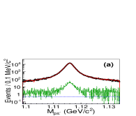
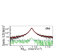
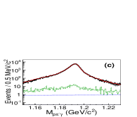
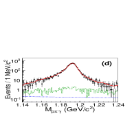
Figure 1: (color online) The $M_{p\pi^{-}}$ distributions for the decays (a) $J/\psi\to\Lambda\bar{\Lambda}$ and (b) $\psi(3686)\to\Lambda\bar{\Lambda}$, and the $M_{p\pi^{-}\gamma}$ distributions for the decays (c) $J/\psi\to\Sigma^{0}\bar{\Sigma}^{0}$ and (d) $\psi(3686)\to\Sigma^{0}\bar{\Sigma}^{0}$, where the dots with error bars are data, the red solid curves are the overall fit results, the green dashed histograms are the backgrounds estimated with the exclusive MC simulated samples, and the blue dotted line describes the remaining backgrounds.

Table 3: The numbers of observed signal events $N_{\text{obs}}$, the corrected detection efficiency $\epsilon$, the numbers of peaking backgrounds $N_{\text{pk}}$, the numbers of smooth backgrounds $N_{\text{sm}}$, the resultant $\alpha$ values for the angular distributions and the branching fractions $\mathcal{B}$, where the errors are statistical only.

Channel	$N_{\text{obs}}$	$\epsilon$ (%)	$N_{\text{pk}}$	$N_{\text{sm}}$	$\alpha$	$\mathcal{B}$ ($\times 10^{-4}$)
$J/\psi\to\Lambda\bar{\Lambda}$	$440,675\pm 670$	$42.37\pm 0.14$	1,819	$154\pm 166$	$0.469\pm 0.026$	$19.43\pm 0.03$
$J/\psi\to\Sigma^{0}\bar{\Sigma}^{0}$	$111,026\pm 335$	$17.83\pm 0.06$	820	$131\pm 12$	$-0.449\pm 0.020$	$11.64\pm 0.04$
$\psi(3686)\to\Lambda\bar{\Lambda}$	$31,119\pm 187$	$42.83\pm 0.34$	252	$352\pm 65$	$0.824\pm 0.074$	$3.97\pm 0.02$
$\psi(3686)\to\Sigma^{0}\bar{\Sigma}^{0}$	$6,612\pm 82$	$14.79\pm 0.12$	89	$17\pm 5$	$0.71\pm 0.11$	$2.44\pm 0.03$

The branching fractions are calculated using

$$\mathcal{B}(\psi\to B\bar{B})=\frac{N_{\text{obs}}}{N_{\psi}\cdot\epsilon\cdot\mathcal{B}_{i}},$$ (3)

where $N_{\text{obs}}$ is the number of signal events minus peaking background; $\epsilon$ is the detection efficiency, which is estimated with MC simulation incorporating the $\cos\theta$ distributions obtained in this analysis and the scale factors to account for the difference in efficiency between data and MC simulation as described below; $\mathcal{B}_{i}$ is the product of branching fractions for the intermediate states in the cascade decay from the PDG Ref:pdg ; and $N_{\psi}$ is the total number of $\psi$ events estimated by counting the inclusive hadronic events Ref:ntot_jpsi ; Ref:ntot_psip . The corresponding detection efficiencies and the resultant branching fractions are also summarized in Table 3.

V.2 Angular distributions

The baryon $\cos\theta$ distributions in the c.m. system corrected by detection efficiency are shown in Fig. 2, and the signal yields in each of the 20 bins are determined with the same method as that in the branching fraction measurements. The detection efficiencies in each bin are estimated with the signal MC samples and scaled with correction factors to compensate for the efficiency difference between data and MC simulation. The efficiency corrected $\cos\theta$ distributions are fitted with Eq. 2 with a least squares method, the corresponding fit results are shown in Fig. 2, and the resultant $\alpha$ values are summarized in Table 3.

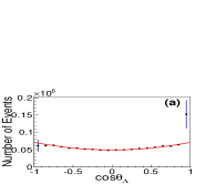
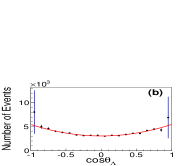
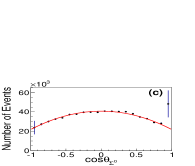
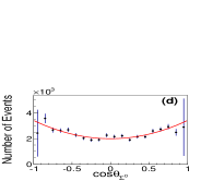
Figure 2: (color online) The distributions of efficiency corrected polar angle of the baryon for the decays (a) $J/\psi\to\Lambda\bar{\Lambda}$, (b) $\psi(3686)\to\Lambda\bar{\Lambda}$, (c) $J/\psi\to\Sigma^{0}\bar{\Sigma}^{0}$, and (d) $\psi(3686)\to\Sigma^{0}\bar{\Sigma}^{0}$, where the dots with error bars are data, and the red solid curves are the fit results.

The correction factors used to correct for the efficiency differences between data and MC simulation as a function of $\cos\theta$ are determined by studying various control samples, where $\theta$ is the polar angle of the hyperon. The efficiency differences are due to differences in the efficiencies of charged particle tracking, photon detection, and hyperon reconstruction. For example, the efficiencies related with charged particle tracking and $\Lambda$ reconstruction are studied with a special control sample of $\psi\to\Lambda\bar{\Lambda}$ events, where a $\bar{\Lambda}$ tag has been reconstructed. Events with two or more charged tracks, in which a $\bar{p}$ and $\pi^{+}$ have been identified using particle identification, are selected. The $\bar{\Lambda}$ tag candidate must satisfy a secondary vertex fit, have a decay length greater than 0.2 cm, and satisfy mass and momentum requirements. The numbers of tagged $\Lambda$ events, $N_{tag}$, are obtained by fitting the $\Lambda$ peak in the distribution of invariant mass recoiling against the $\bar{\Lambda}$ tag. The numbers of $\Lambda$ signal events, $N_{sig}$, are obtained by fitting the recoil mass distribution for events where, in addition, a $\Lambda$ signal is reconstructed on the recoil side, which requires two oppositely charged tracks that satisfy a vertex fit and have a decay length greater than 0.2 cm. The combined efficiency of charged tracking (proton and pion) and $\Lambda$ reconstruction is then $N_{sig}/N_{tag}$. The ratios of the data and MC simulation efficiencies as a function of $\cos\theta$ are taken as the correction factors. The $\bar{\Lambda}$ correction factors are determined in an analogous way using $\psi\to\Lambda\bar{\Lambda}$ events with a $\Lambda$ tag. The overall correction factor in the different $\cos\theta$ bins is the product of the $\Lambda$ and $\bar{\Lambda}$ correction factors.

In an analogous way, the combined efficiency of photon detection and $\Sigma^{0}$ reconstruction is studied with a control sample of $\psi\to\Sigma^{0}\bar{\Sigma}^{0}$ events, which have a $\bar{\Sigma}^{0}$ tag and an additional $\Lambda$. Events are selected that have a $\Lambda$ and $\bar{\Lambda}$ using the same criteria as above and at least one additional photon. The $\bar{\Lambda}$ and photon must have an invariant mass consistent with that of a $\bar{\Sigma}^{0}$. The numbers of tagged $\Sigma^{0}$ events are obtained by fitting the $\Sigma^{0}$ peak in the distribution of mass recoiling against the $\bar{\Sigma}^{0}$ tag. We then search for another photon and reconstruct the $\Sigma^{0}$ by requiring the invariant mass of the photon and tagged $\Lambda$ be consistent with the $\Sigma^{0}$ mass. The number of events with a $\Sigma^{0}$ signal divided by the number of tagged $\Sigma^{0}$ events is the combined efficiency of photon detection and $\Sigma^{0}$ reconstruction. The ratios of detection efficiencies in the different $\cos\theta$ bins between data and MC simulation, determine the correction factors. The overall correction factor in the different $\cos\theta$ bins is the product of the $\Sigma^{0}$, $\bar{\Sigma}^{0}$, $\Lambda$, and $\bar{\Lambda}$ correction factors.

VI SYSTEMATIC UNCERTAINTY

VI.1 Branching Fraction

Systematic uncertainties in the branching fraction measurements are mainly due to the differences of detection efficiency and resolution between data and MC simulation. The sources of uncertainty related with the detection efficiency include charged tracking, photon detection, and $\Lambda$/$\Sigma^{0}$ reconstruction. The sources of uncertainty due to the resolution difference include the $M_{\Lambda\bar{\Lambda}}$ and $M_{\bar{\Lambda}}/M_{\bar{\Sigma}^{0}}$ mass requirements, and the opening angle $\theta_{\Sigma^{0}\bar{\Sigma}^{0}}$ requirement in the decays $\psi\to\Sigma^{0}\bar{\Sigma}^{0}$. Additional uncertainty sources including the model of the baryon polar angular distribution, the fit procedure, the decay branching fractions of $\Lambda$/$\Sigma^{0}$ states and the total number of $\psi$ events are also considered. All of systematic uncertainties are studied in detail as discussed in the following:

1. As described above, the detection efficiencies related with the tracking, photon detection, and $\Lambda$/$\Sigma^{0}$ reconstruction are corrected bin-by-bin in $\cos\theta$ to decrease the difference between data and MC simulation. The overall correction factors, which are determined with control samples are $0.9974\pm 0.0041$, $0.9936\pm 0.0064$, $0.980\pm 0.011$, and $0.954\pm 0.022$ for the decays $J/\psi\to\Lambda\bar{\Lambda}$, $J/\psi\to\Sigma^{0}\bar{\Sigma}^{0}$, $\psi(3686)\to\Lambda\bar{\Lambda}$ and $\psi(3686)\to\Sigma^{0}\bar{\Sigma}^{0}$, respectively. To estimate the corresponding uncertainties, the correction factors are changed by $\pm$1 standard deviations, and the resultant changes in the branching fractions are taken as the systematic uncertainties.

2. The uncertainties related with the $M_{\Lambda\bar{\Lambda}}$ requirement are estimated by varying the mass requirement edges by $\pm 10$ MeV/$c^{2}$. The uncertainties related with the $\bar{\Lambda}/\bar{\Sigma}^{0}$ mass requirement are estimated by changing the requirement by $\pm 1$ times the mass resolution. The uncertainties due to the requirement on the opening angle $\theta_{\Sigma^{0}\bar{\Sigma}^{0}}$ in the decays $\psi\to\Sigma^{0}\bar{\Sigma}^{0}$ are estimated by changing the requirement to be 175^∘. The relative changes in the branching fractions are individually taken as the systematic uncertainties.

3. MC simulations indicate that the detection efficiencies depend on the distributions of baryon polar angular $\cos\theta$. In the analysis, the measured $\alpha$ values are used for the $\cos\theta$ distributions in the MC simulation. Alternative MC samples are generated by changing the $\alpha$ values by $\pm 1$ standard deviations and are used to estimate the detection efficiencies. The resultant changes in the detection efficiencies with respect to their nominal values are taken as the systematic uncertainties.

4. The sources of systematic uncertainty associated with the fit procedure include the fit range, the signal shape and the modeling of backgrounds. The uncertainties related with the fit range are estimated by changing the range by $\pm 1$ times the mass resolution for the fits. The signal shapes are modeled with the signal MC simulated shapes convolved with a Gaussian function in the nominal fit. The corresponding uncertainties are estimated with alternative fits with different signal shapes, $i.e.$, a Breit-Wigner function convolved with a Gaussian function for $\Lambda$ and with a Crystal Ball function Ref:cball for $\Sigma^{0}$, where the Gaussian function and Crystal Ball function represent the corresponding mass resolutions. The uncertainties related with the peaking backgrounds, which are estimated with the exclusive MC samples in the nominal fits, are studied by changing the branching fractions of the individual background, or by changing the branching fractions for the reference decays which the estimated branching fractions for the undetermined backgrounds are based on, by $\pm 1$ times their uncertainties from the PDG Ref:pdg . The uncertainties associated with the non-peaking backgrounds are estimated with alternative fits by replacing the second order polynomial function with a first order polynomial function. The resultant changes from the above changes in the signal yields are taken individually as the systematic uncertainties.

5. The uncertainties related with the branching fractions of baryon and anti-baryon decays are taken from the PDG Ref:pdg . The total numbers of $\psi$ events are obtained by studying the inclusive hadronic events, and their uncertainties are 0.6% and 0.7% for the $J/\psi$ and $\psi(3686)$ data samples Ref:ntot_jpsi ; Ref:ntot_psip , respectively.

The various systematic uncertainties in the branching fraction measurements are summarized in Table 4. The total systematic uncertainties are obtained by summing the individual values in quadrature.

Table 4: Systematic uncertainties in the measurement of branching fractions (%).

	$J/\psi$		$\psi(3686)$
	$\Lambda\bar{\Lambda}$	$\Sigma^{0}\bar{\Sigma}^{0}$	$\Lambda\bar{\Lambda}$	$\Sigma^{0}\bar{\Sigma}^{0}$
Efficiency correction	0.5	0.7	1.2	2.3
$M_{\Lambda\bar{\Lambda}}$ requirement	0.1	0.1	0.1	0.2
$\bar{\Lambda}/\bar{\Sigma}^{0}$ mass requirement	0.1	0.3	0.3	0.2
$\theta_{\Sigma^{0}\bar{\Sigma}^{0}}$ requirement	$-$	0.3	$-$	0.2
Baryon polar angle	0.8	0.9	2.0	3.1
Fit range	0.1	0.1	0.2	0.2
Signal shape	0.1	0.3	0.1	0.2
Peaking bkg.	0.3	0.4	0.3	1.2
Non-peaking bkg.	0.1	0.1	0.3	0.2
Branching fractions	1.2	1.2	1.2	1.2
$N_{J/\psi}/N_{\psi(3686)}$	0.6	0.6	0.7	0.7
Total	1.7	1.9	2.8	4.3

VI.2 Angular Distribution

The sources of systematic uncertainties in the baryon polar angular measurements include the signal yields in different $\cos\theta$ intervals and the $\cos\theta$ fit procedure. The MC statistics and correction errors are already included in the error referred to as “statistical”.

1. In the polar angular measurements, the signal yield in a given $\cos\theta$ interval is obtained with the same fit method as that used in the branching fraction measurements. The uncertainties of the signal yield in each $\cos\theta$ bin are mainly from the fit range, the signal shape and the background modeling. We individually estimate the uncertainty of the signal yield in each $\cos\theta$ interval with the same methods as those used in the branching fraction measurements for the different uncertainty sources, and then repeat the $\cos\theta$ fit procedure with the changed signal yields. The resultant changes in the $\alpha$ values with respect to the nominal values are taken as systematic uncertainties.

2. The sources of systematic uncertainty related to the $\cos\theta$ fit procedure include the fit range and the number of bins in the $\cos\theta$ distribution. We repeat the fit procedures with the alternative fit range $[-0.9,0.9]$ and alternative number of bins (40). The resultant changes of $\alpha$ values are taken as the systematic uncertainties.

The individual absolute uncertainties in the polar angular distribution measurements are summarized in Table 5. The total systematic uncertainties are obtained by summing the individual values in quadrature.

Table 5: Absolute systematic uncertainties in the measurement of $\alpha$.

	$J/\psi$		$\psi(3686)$
	$\Lambda\bar{\Lambda}$	$\Sigma^{0}\bar{\Sigma}^{0}$	$\Lambda\bar{\Lambda}$	$\Sigma^{0}\bar{\Sigma}^{0}$
Mass fit range	0.001	0.001	0.003	0.005
Signal shape	0.001	0.002	0.001	0.003
Peaking bkg.	0.006	0.005	0.006	0.015
Non-peaking bkg.	0.002	0.001	0.004	0.002
$\alpha$ fit range	0.001	0.003	0.007	0.019
Number of bins	0.004	0.005	0.001	0.024
Total	0.008	0.008	0.011	0.035

VII Summary

In summary, using the data samples of $1310.6\times 10^{6}$ $J/\psi$ events and $447.9\times 10^{6}$ $\psi(3686)$ events collected with the BESIII detector at the BEPCII collider, the $J/\psi$ and $\psi(3686)$ decaying into $\Lambda\bar{\Lambda}$ and $\Sigma^{0}\bar{\Sigma}^{0}$ pairs are studied. The decay branching fractions and $\alpha$ values are measured, and the results are summarized in Table 6. The branching fractions for $J/\psi$ decays are in good agreement with the results of BESII Ref:bes_2006 and BaBar Ref:babar_2007 experiments, and those for $\psi(3686)$ decays are in agreement with the results of CLEO Ref:cleo_2005 , BESII Ref:bes_2007 and S. Dobbs et al. Ref:cleo_2014 with a maximum of 2 times of standard deviations. The earlier experimental results Ref:markii_1984 ; Ref:dm2_1987 ; Ref:bes_1998 ; Ref:bes_2001 have significant differences with those of this analysis. The precisions of our branching fraction results are much improved than those of previous experiments listed in Table 1. The $\alpha$ values in the decays $\psi(3686)\to\Lambda\bar{\Lambda}$ and $\psi(3686)\to\Sigma^{0}\bar{\Sigma}^{0}$ are measured for the first time, while those of $J/\psi\to\Lambda\bar{\Lambda}$ and $J/\psi\to\Sigma^{0}\bar{\Sigma}^{0}$ decays are of much improved precision compared to previous measurements. It is worth noting that the $\alpha$ value in the decay $J/\psi\to\Sigma^{0}\bar{\Sigma}^{0}$ is negative, which confirms the results in Ref. Ref:bes_2006 .

Table 6: Results for measured $\alpha$ values and branching fractions $\mathcal{B}$ in this analysis. The first uncertainties are statistical, and the second are systematic.

Channel	$\alpha$	$\mathcal{B}$ ($\times 10^{-4}$)
$J/\psi\to\Lambda\bar{\Lambda}$	$0.469\pm 0.026\pm 0.008$	$19.43\pm 0.03\pm 0.33$
$J/\psi\to\Sigma^{0}\bar{\Sigma}^{0}$	$-0.449\pm 0.020\pm 0.008$	$11.64\pm 0.04\pm 0.23$
$\psi(3686)\to\Lambda\bar{\Lambda}$	$0.82\pm 0.08\pm 0.02$	$3.97\pm 0.02\pm 0.12$
$\psi(3686)\to\Sigma^{0}\bar{\Sigma}^{0}$	$0.71\pm 0.11\pm 0.04$	$2.44\pm 0.03\pm 0.11$

To test the “12% rule”, we also obtain the Q values to be $\frac{\mathcal{B}(\psi(3686)\to\Lambda\bar{\Lambda})}{\mathcal{B}(J/\psi\to\Lambda\bar{\Lambda})}=~{}$($20.43\pm 0.11\pm 0.58$)% and $\frac{\mathcal{B}(\psi(3686)\to\Sigma^{0}\bar{\Sigma}^{0})}{\mathcal{B}(J/\psi\to\Sigma^{0}\bar{\Sigma}^{0})}=~{}$($20.96\pm 0.27\pm 0.92$)%, where the common systematic uncertainties between $J/\psi$ and $\psi(3686)$ decays are cancelled. The Q values are of high precision, and differ from the expectation from pQCD by more than 3 standard deviations.

VIII Acknowledgments

The BESIII collaboration thanks the staff of BEPCII and the IHEP computing center for their strong support. This work is supported in part by National Key Basic Research Program of China under Contract Nos. 2009CB825200, 2015CB856700; National Natural Science Foundation of China (NSFC) under Contracts Nos. 10905034, 10935007, 11125525, 11235011, 11322544, 11335008, 11425524; the Chinese Academy of Sciences (CAS) Large-Scale Scientific Facility Program; the CAS Center for Excellence in Particle Physics (CCEPP); the Collaborative Innovation Center for Particles and Interactions (CICPI); Joint Large-Scale Scientific Facility Funds of the NSFC and CAS under Contracts Nos. 11179007, U1232106, U1232201, U1332201; Natural Science Foundation of Shandong Province under Contract No. ZR2009AQ002; CAS under Contracts Nos. KJCX2-YW-N29, KJCX2-YW-N45; 100 Talents Program of CAS; National 1000 Talents Program of China; INPAC and Shanghai Key Laboratory for Particle Physics and Cosmology; German Research Foundation DFG under Contract No. Collaborative Research Center CRC-1044, FOR-2359; Istituto Nazionale di Fisica Nucleare, Italy; Joint Funds of the National Science Foundation of China under Contract No. U1232107; Ministry of Development of Turkey under Contract No. DPT2006K-120470; Russian Foundation for Basic Research under Contract No. 14-07-91152; The Swedish Resarch Council; U. S. Department of Energy under Contracts Nos. DE-FG02-04ER41291, DE-FG02-05ER41374, DE-SC0012069, DESC0010118; U.S. National Science Foundation; University of Groningen (RuG) and the Helmholtzzentrum fuer Schwerionenforschung GmbH (GSI), Darmstadt; WCU Program of National Research Foundation of Korea under Contract No. R32-2008-000-10155-0.

References

- (1) P. Kessler, Nucl. Phys. B 15, 253-266 (1970); S. J. Brodsky and G. P. Lepage, Phys. Rev. D 24, 2848 (1981).
- (2) T. Appelquist and H. D. Politzer, Phys. Rev. Lett. 34, 43 (1975); A. De Rujula and S. L. Glashow, Phys. Rev. Lett. 34, 46 (1975); W. S. Hou, Phys. Rev. D 55, 6952 (1997).
- (3) M. E. B. Franklin et al. (MARKII Collaboration), Phys. Rev. Lett. 51, 963 (1983).
- (4) K. A. Olive et al. (Particle Data Group), Chin. Phys. C 38, 090001 (2014).
- (5) Y. F. Gu and X. H. Li, Phys. Rev. D 63, 114019 (2001); X. H. Mo, C. Z. Yuan and P. Wang, High Energy Physics and Nuclear Physics 31, 686 (2007); N. Brambilla et al. (Quarkonium Working Group), Eur. Phys. J. C 71, 1534 (2011); Q. Wang, G. Li and Q. Zhao, Phys. Rev. D 85, 074015 (2012).
- (6) M. W. Eaton et al. (MARKII Collaboration), Phys. Rev. D 29, 804 (1984).
- (7) D. Pallin et al. (DM2 Collaboration), Nucl. Phys. B 292, 653 (1987).
- (8) J. Z. Bai et al. (BES Collaboration), Phys. Lett. B 424, 213 (1998).
- (9) J. Z. Bai et al. (BES Collaboration), Phys. Rev. D 63, 032002 (2001).
- (10) T. K. Pedlar et al. (CLEO Collaboration), Phys. Rev. D 72, 051108 (2005).
- (11) M. Ablikim et al. (BESII Collaboration), Phys. Lett. B 632, 181 (2006).
- (12) M. Ablikim et al. (BESII Collaboration), Phys. Lett. B 648, 149 (2007).
- (13) B. Aubert et al. (BaBar Collaboration), Phys. Rev. D 76, 092006 (2007).
- (14) S. Dobbs et al., Phys. Lett. B 739, 90 (2014).
- (15) M. Ablikim et al. (BESIII Collaboration), Phys. Rev. D 93, 072003 (2016); M. Ablikim et al. (BESIII Collaboration), arXiv:1612.08664.
- (16) M. Claudson, S. L. Glashow and M. B. Wise, Phys. Rev. D 25, 1345 (1982).
- (17) C. Carimalo, Int. J. Mod. Phys. A 2, 249 (1987).
- (18) M. Ablikim et al. (BESIII Collaboration), Chin. Phys. C 36, 915 (2012); M. Ablikim et al. (BESIII Collaboration), arXiv:1607.00738, (to be published on Chin. Phys. C).
- (19) M. Ablikim et al. (BESIII Collaboration), Chin. Phys. C 37, 063001 (2013); The total number of events taken at 2009 and 2012 is obtained based on the same method. The preliminary number is determined to be with uncertainties of 0.7%.
- (20) M. Ablikim et al. (BESIII Collaboration), Nucl. Instrum. Meth. A 614, 345 (2010).
- (21) C. Zhang, Sci. China G 53, 2084 (2010).
- (22) D. M. Asner et al., Int. J. Mod. Phys. A 24, 499 (2009).
- (23) S. Agostinelli et al. (GEANT4 Collaboration), Nucl. Instrum. Meth. A 506, 250 (2003).
- (24) Z. Y. Deng et al., HEP & NP 30, 371 (2006).
- (25) W. D. Li, Y. J. Mao and Y. F. Wang, Int. J. Mod. Phys. A 24S1, 9 (2009).
- (26) S. Jadach, B. F. L. Ward and Z. Was, Comp. Phys. Commu. 130, 260 (2000); Phys. Rev. D 63, 113009 (2001).
- (27) D. J. Lange, Nucl. Instrum. Meth. A 462, 152 (2001); R. G. Ping, Chin. Phys. C 32, 599 (2008).
- (28) J. C. Chen, G. S. Huang, X. R. Qi, D. H. Zhang and Y. S. Zhu, Phys. Rev. D 62, 034003 (2000).
- (29) M. Xu et al., Chin. Phys. C 33, 428 (2009).
- (30) M. Ablikim et al. (BESIII Collaboration), Phys. Rev. D86, 032014 (2012).
- (31) J. Cheng, Z. Wang, L. Lebanowski, G. Lin and S. Chen, Nucl. Instrum. Meth. A 827, 165 (2016).