Stage-parallel fully implicit Runge-Kutta solvers for discontinuous Galerkin fluid simulations

Abstract

In this paper, we develop new techniques for solving the large, coupled linear systems that arise from fully implicit Runge-Kutta methods. This method makes use of the iterative preconditioned GMRES algorithm for solving the linear systems, which has seen success for fluid flow problems and discontinuous Galerkin discretizations. By transforming the resulting linear system of equations, one can obtain a method which is much less computationally expensive than the untransformed formulation, and which compares competitively with other time-integration schemes, such as diagonally implicit Runge-Kutta (DIRK) methods. We develop and test several ILU-based preconditioners effective for these large systems. We additionally employ a parallel-in-time strategy to compute the Runge-Kutta stages simultaneously. Numerical experiments are performed on the Navier-Stokes equations using Euler vortex and 2D and 3D NACA airfoil test cases in serial and in parallel settings. The fully implicit Radau IIA Runge-Kutta methods compare favorably with equal-order DIRK methods in terms of accuracy, number of GMRES iterations, number of matrix-vector multiplications, and wall-clock time, for a wide range of time steps.

Keywords: implicit Runge-Kutta; discontinuous Galerkin; preconditioned GMRES; parallel-in-time

1 Introduction

The discontinuous Galerkin method, introduced in 1973 by Reed and Hill for the neutron transport equation [29], has seen in recent years increased interest for fluid dynamics applications [24]. The discontinuous Galerkin method is a high-order finite element method suitable for use on unstructured meshes with polynomials of arbitrarily high degree. For many fluid flow problems, explicit time integration methods have the downside of restrictive time step conditions, partly because of the use of high-degree polynomials but more fundamentally because of the need to employ highly graded and/or anisotropic elements for many realistic flow problems [27]. Therefore, for many applications it is desirable to use an implicit time integration scheme.

Implicit time integration methods for DG have been much studied. Multi-step backward differentiation formulas (BDF) and single-step diagonally implicit Runge-Kutta (DIRK) methods have been applied to discontinuous Galerkin discretizations for fluid flow problems [26, 27]. Nigro et. al have seen success applying multi-stage, multi-step modified extended BDF (MEBDF) and two implicit advanced step-point (TIAS) schemes to the compressible Euler and Navier-Stokes equations [21, 22]. Additionally, in [3], Bassi et al. have used linearly implicit Rosenbrock-type to integrate DG discretizations for various fluid flow problems. The BDF and DIRK methods have some limitations: BDF schemes can be $A$-stable only up to second-order (the famous second Dahlquist barrier) [10], a severe limitation when used in conjunction with a high-order spatial discretization. On the other hand, there exist high-order $A$-stable (and even $L$-stable) DIRK schemes, but these methods have a low stage-order, often resulting in order reduction when applied to stiff problems [13].

The Radau IIA methods, one class of the so-called fully implicit Runge-Kutta (IRK) methods, are high-order, $L$-stable, and have relatively high stage order. Consequently, these methods suffer less from order reduction than the corresponding DIRK methods when applied to stiff problems. Furthermore, these methods require only a small number of stages $s$, with the order of accuracy given by $p=2s-1$. These methods have the drawback that each step involves the solution of large, coupled linear systems of equations. The difficulty in efficiently implementing such methods has caused them to remain not widely used or studied for practical applications [8, 9]. There has been previous work on improving the efficiency of solving these large, coupled systems. In [16], Jay and Braconnier develop a parallelizable preconditioner for IRK methods by means of Hairer and Wanner’s $W$-transformation. In [11], De Swart et al. have developed a parallel software package for the four-stage Radau IIA method, and Burrage et at. have developed a matrix-free, parallel implementation of the fifth-order Radau IIA method in [6].

In this paper, we develop a new strategy for efficiently solving the resulting large linear systems by means of the iterative preconditioned GMRES algorithm. A simple transformation of the linear system results in a significant reduction of the cost per GMRES iteration. Furthermore, the block ILU(0) preconditioner, used successfully with implicit time-integrators for the discontinuous Galerkin method in [28], proves to be effective also for these large systems. A shifted, uncoupled, block ILU(0) factorization is also found to be an effective preconditioner, with the advantage of allowing parallelism in time by computing the stage solutions simultaneously.

The structure of this paper is as follows. In Section 2, we describe the governing equations and DG spatial discretization. In Section 3, we discuss the time integration schemes used in this paper. Then, in Section 4, we introduce the transformation used to reduce the solution cost, and discuss the preconditioners used for the GMRES method. Finally, in Section 5, we perform numerical experiments on a variety of test cases, in two and three spatial dimensions.

2 Equations and spatial discretization

The equations considered are the time-dependent, compressible Navier-Stokes equations,

$$\frac{\partial\rho}{\partial t}+\frac{\partial}{\partial x_{j}}(\rho u_{j})=0$$ (1)

$$\frac{\partial}{\partial t}(\rho u_{i})+\frac{\partial}{\partial x_{j}}(\rho u_{i}u_{j})+\frac{\partial p}{\partial x_{i}}=\frac{\partial\tau_{ij}}{\partial x_{j}}\qquad\text{for $i=1,2,3,$}$$ (2)

$$\frac{\partial}{\partial t}(\rho E)+\frac{\partial}{\partial x_{j}}\left(u_{j}(\rho E+p)\right)=-\frac{\partial q_{j}}{\partial x_{j}}+\frac{\partial}{\partial x_{j}}(u_{i}\tau_{ij}),$$ (3)

where $\rho$ is the density, $u_{i}$ is the $i$th component of the velocity, and $E$ is the total energy. The viscous stress tensor and heat flux are given by

$$\tau_{ij}=\mu\left(\frac{\partial u_{i}}{\partial x_{j}}+\frac{\partial u_{j}}{\partial x_{i}}-\frac{2}{3}\frac{\partial u_{k}}{\partial x_{k}}\delta_{ij}\right)\qquad\text{and}\qquad q_{j}=-\frac{\mu}{\rm Pr}\frac{\partial}{\partial x_{j}}\left(E+\frac{p}{\rho}-\frac{1}{2}u_{k}u_{k}\right),$$ (4)

where $\mu$ is the viscosity coefficient, and ${\rm Pr}=0.72$ is the Prandtl number. For an ideal gas, the pressure $p$ is given by the equation of state

$$p=(\gamma-1)\rho\left(E-\frac{1}{2}u_{k}u_{k}\right),$$ (5)

where $\gamma$ is the adiabatic gas constant. For the viscous problems, we introduce an isentropic assumption of the form $p=K\rho^{\gamma},$ for a given constant $K$, as described in [17]. This additional simplification can be thought of as an artificial compressibility model for the incompressible flows simulated in Sections 5.2 and 5.3. We prefer to solve the compressible equations because they result in a system of ODEs rather than differential-algebraic equations, and thus do not need specialized projection-type solvers. This model decouples equation (3) from equations (1) and (2), and therefore results in one fewer component to solve for. We remark that this simplification does not result in a significant difference in the relative performance of the time integrators studied in this paper, as shown in Section (5.1), where the full compressible Euler equations are solved, with no isentropic assumption.

We rewrite equations (1), (2), and (3) in the form

$$\frac{\partial u}{\partial t}+\nabla\cdot\bm{F}_{i}(u)-\nabla\cdot\bm{F}_{v}(u,\nabla u)=0,$$ (6)

where $u$ is a vector of the conserved variables, and $\bm{F}_{i},\bm{F}_{v}$ are the inviscid and viscous flux functions, respectively. The spatial domain $\Omega$ is discretized into a triangulation, and the solution $u$ is approximated by piecewise polynomials of a given degree. Equation (6) is discretized by means of the discontinuous Galerkin method, where the viscous terms are treated using the compact DG (CDG) scheme [23].

Using a nodal basis function for each component, we write the global solution vector as $\bm{u}$, and obtain a semi-discrete system of ordinary differential equations of the form

$$\bm{M}\frac{\partial\bm{u}}{\partial t}=\bm{f}(\bm{u}),$$ (7)

where $\bm{M}$ is the mass matrix, and $\bm{f}$ is a nonlinear function of the $n$ unknowns $\bm{u}$. The standard method of lines approach allows for the solution of this system of ordinary differential equations by means of a range of numerical time integrators, such as the implicit Runge-Kutta methods that are the focus of this paper.

2.1 Block structure of the Jacobian

We consider the vector of unknowns $\bm{u}$ to be ordered such that the $m$ degrees of freedom associated with one element of the triangulation appear consecutively. We suppose that there are a total of $T$ elements, such that there are a total of $n=Tm$ degrees of freedom. Then, the Jacobian matrix $\bm{J}$ can be seen as a $T\times T$ block matrix, with blocks of size $m\times m$. The $i$th row consists of blocks on the diagonal, and in columns $j$, where elements $i$ and $j$ share a common edge, such that the total number of off-diagonal blocks in the $i$th row is equal to the number of neighbors of element $i$. We note that the off-diagonal blocks of size $m\times m$ are themselves sparse, but for the sake of simplicity we will consider them as dense matrices. The mass matrix $\bm{M}$ is a $T\times T$ block diagonal matrix, with blocks of size $m\times m$, and therefore matrices of the form $\alpha\bm{M}-\beta\bm{J}$ have the same sparsity pattern as the Jacobian.

3 Time integration

In this paper, we will focus on the one-step, multi-stage Runge-Kutta methods. Given initial conditions $\bm{u}_{0}=\bm{u}(t_{0})$, a general $s$-stage, $p$th-order Runge-Kutta method for advancing the solution to $\bm{u}_{1}=\bm{u}(t_{0}+\Delta t)+\mathcal{O}(\Delta t^{p+1})$ can be written as

$$\bm{M}\bm{k}_{i} =\bm{f}\left(t_{0}+\Delta tc_{i},\bm{u}_{0}+\Delta t\sum_{j=1}^{s}a_{ij}\bm{k}_{j}\right),$$ (8)

$$\bm{u}_{1} =\bm{u}_{0}+\Delta t\sum_{i=1}^{s}b_{i}\bm{k}_{i},$$ (9)

where the coefficients $a_{ij},b_{i},$ and $c_{i}$ can be expressed compactly in the form of the Butcher tableau,

$$\begin{array}[]{c|ccc}c_{1}&a_{11}&\cdots&a_{1s}\\ \vdots&\vdots&\ddots&\vdots\\ c_{s}&a_{s1}&\cdots&a_{ss}\\ \hline\cr&b_{1}&\cdots&b_{s}\end{array}={\begin{array}[]{c|c}\bm{c}&\bm{A}\\ \hline\cr&\bm{b}^{T}\end{array}}.$$

If the matrix of coefficients $\bm{A}$ is strictly lower-triangular, then each stage $\bm{k}_{i}$ only depends on the preceding stages, and the method is called an explicit Runge-Kutta method. In this case, each stage may be computed by simply evaluating the function $\bm{f}$. If $\bm{A}$ is not strictly lower-triangular, the method is called an implicit Runge-Kutta method (IRK). A particular class of implicit Runge-Kutta methods is those for which the matrix $\bm{A}$ is lower-triangular. Such methods are called diagonally-implicit Runge-Kutta (DIRK) methods [1]. Implicit Runge-Kutta methods enjoy high accuracy and very favorable stability properties, but computing the stages requires the solution of (in general nonlinear) systems of equations. In the case of DIRK methods, since $\bm{A}$ is lower-triangular, each stage $\bm{k}_{i}$ depends only on those stages $\bm{k}_{j}$, $j\leq i$, requiring the sequential solution of $s$ systems, each of size $n$. In contrast, general IRK methods couple all of the stages, resulting in one nonlinear system of equations of size $s\times n$.

For the solution of stiff systems of equations, we are interested in those methods that are $L$-stable, meaning that their stability region includes the entire left half-place ($A$-stability), together with the additional criterion that the stability function $R(z)$ satisfies $\lim_{z\to\infty}R(z)=0$. In the present study, we compare the efficiency and effectiveness of several $L$-stable IRK and DIRK schemes. The methods considered are listed in Table 1. The IRK schemes considered are the Radau IIA schemes, which are $L$-stable, $s$-stage schemes of order $2s-1$ based on the Radau right quadrature. The construction of these schemes can be found in [15]. The two-stage and three-stage Radau IIA methods are listed as RADAU23 and RADAU35, respectively. The DIRK schemes considered are the three-stage, third-order $L$-stable scheme denoted DIRK33, which is derived in detail in [1], and the six-stage, fifth-order scheme constructed in [5], and denoted ESDIRK65. The latter scheme is an explicit singly diagonally implicit Runge-Kutta (ESDIRK) method, meaning that the first diagonal entry of the Butcher matrix is zero, and the remaining diagonally entries are nonzero and equal. In addition to the third- and fifth-order methods, we also consider the seventh- and ninth-order Radau IIA methods, although we do not compare these methods to equal-order DIRK methods. The Butcher tableaux for the methods considered are given in Appendix A.

Table 1: $L$-stable implicit Runge-Kutta schemes considered

Scheme	Order	Total stages	Implicit stages	Stage order	Leading error coefficient
RADAU23	3	2	2	2	$1.39\times 10^{-2}$
DIRK33	3	3	3	1	$2.59\times 10^{-2}$
RADAU35	5	3	3	3	$1.39\times 10^{-4}$
ESDIRK65	5	6	5	2	$5.30\times 10^{-4}$
RADAU47	7	4	4	4	$7.09\times 10^{-7}$
RADAU59	9	5	5	5	$2.19\times 10^{-9}$

Also of interest is the phenomenon of order reduction, whereby, when applied to stiff problems, the overall order of accuracy is reduced from $p$ to the stage order of the method (denoted $q$) [13]. The stage order $q$ is defined as $q=\min\{p,q_{i}\}$, for $i=1,\ldots,s$, where $q_{i}$ is defined by

$$\bm{u}(t_{0}+\Delta tc_{i})=\bm{u}_{0}+\Delta t\sum_{j=1}^{s}a_{ij}\bm{k}_{j}+\mathcal{O}(\Delta t^{q_{i}+1}).$$ (10)

It can be shown that the maximum stage order for any DIRK method is 2 [14], whereas the stage order for the Radau IIA methods is given by the number of stages, $q=s$ [19]. The DIRK33 has stage order of $q=1$. An advantage of the ESDIRK methods such as ESDIRK65 is that they have stage order of $q=2$ [18].

The Radau IIA methods are very attractive because of their high order of accuracy, small number of stages, high stage order, and $L$-stability, but solving the coupled system of $s\times n$ equations is computationally expensive. Supposing that we solve the nonlinear system of equations for the stages $\bm{k}_{i}$ by means of Newton’s method, then at each iteration we must solve a linear system of equations by inverting the Jacobian matrix of the right-hand side, $\bm{f}(t,\bm{u})$. Assuming a dense Jacobian matrix, and solution via Gaussian elimination (or LU factorization), then the cost of performing a linear solve scales as the cube of the number of unknowns. Therefore, the cost per linear solve for a general IRK method is $\mathcal{O}(s^{3}n^{3})$, whereas the cost per solve for a DIRK method scales like $\mathcal{O}(sn^{3})$. In [7], Butcher describes how to transform the resulting set of linear equations to reduce the computational work for solving the IRK systems to $\mathcal{O}(2sn^{3})$. Despite this reduction in computational complexity, the cost of solving the large systems of equations has proven in practice to be prohibitive [8]. On the other hand, DIRK methods have proven be popular and effective for solving computational fluid dynamics problems [4], at the cost of lower stage order and an increased number of stages.

4 Efficient solution of implicit Runge-Kutta systems

In this section we describe a method for efficiently solving the systems arising from general IRK methods when applied to discontinuous Galerkin discretizations. The Jacobian matrices of the function $\bm{f}$ are sparse, block-structured matrices, which lend themselves to solution via iterative Krylov subspace methods. In particular, we consider the solution of these systems by means of the GMRES method with a zero fill-in block ILU(0) preconditioner, as in [28]. In this case, each iteration of the GMRES method requires one matrix-vector multiplication, and one application of the ILU(0) preconditioner. In order to efficiently solve the linear systems resulting from IRK methods, we will rewrite the system of equations in such a way so as to reduce the cost of a matrix-vector multiplication from $s^{2}n^{2}$ to order $sn^{2}$.

4.1 Transformation of the system of equations

Recalling equation that the stages $\bm{k}_{i}$ are given by the equation

$$\bm{M}\bm{k}_{i}=\bm{f}\left(t_{0}+\Delta tc_{i},\bm{u}_{0}+\Delta t\sum_{j=1}^{s}a_{ij}\bm{k}_{j}\right),$$ (11)

we define $\bm{K}$ to be the concatenation of the vectors $\bm{k}_{i}$, $\bm{U}_{0}$ to be the concatenation of $s$ copies of $\bm{u}_{0}$, and $\bm{F}$ the function $\bm{f}$ applied component-wise on these vectors. Then, we rewrite equation (11) in vector form as

$$(\bm{I}_{s}\otimes\bm{M})\bm{K}=\bm{F}\left(t_{0}+\Delta t\bm{c},\bm{U}_{0}+\Delta t(\bm{A}\otimes\bm{I}_{n})\bm{K}\right),$$ (12)

where $\otimes$ is the Kronecker product, and $\bm{I}_{n}$ is the $n\times n$ identity matrix.

This nonlinear system can be solved by means of Newton’s method, which will require solving at each step a linear system of the form

$$\left(\left(\begin{array}[]{ccc}\bm{M}&&0\\ &\ddots&\\ 0&&\bm{M}\end{array}\right)-\Delta t\left(\begin{array}[]{ccc}a_{11}\bm{J}_{1}&\cdots&a_{1s}\bm{J}_{1}\\ \vdots&\ddots&\vdots\\ a_{s1}\bm{J}_{s}&\cdots&a_{ss}\bm{J}_{s},\end{array}\right)\right)\left(\begin{array}[]{ccc}\bm{k}_{1}\\ \vdots\\ \bm{k}_{s}\end{array}\right)=\left(\begin{array}[]{ccc}\bm{r}_{1}\\ \vdots\\ \bm{r}_{s}\end{array}\right)$$ (13)

for the residual vectors $(\bm{r}_{1},\ldots,\bm{r}_{s})^{T}$, where the matrices on the left-hand side are $s\times s$ block matrices blocks, with each block of size $n\times n$. We use the following notation for the Jacobian matrix of $\bm{f}$,

$$\bm{J}_{i}=\bm{J}_{\bm{f}}\left(t_{0}+\Delta tc_{i},\bm{u_{0}}+\Delta t\sum_{j=1}^{s}a_{ij}\bm{k}_{j}\right).$$

We can rewrite equation (13) in the following form,

$$\left(\bm{I}_{s}\otimes\bm{M}-\Delta t\left(\begin{array}[]{ccc}a_{11}J_{1}&\cdots&a_{1s}J_{1}\\ \vdots&\ddots&\vdots\\ a_{s1}J_{s}&\cdots&a_{ss}J_{s}\end{array}\right)\right)\bm{K}=\bm{R},$$ (14)

The sparsity pattern of the matrix in (14) is simply that of the Jacobian matrix $J$ repeated $s\times s$ times, and we can conclude that the cost of computing a matrix-vector product with this matrix is $s^{2}$ times that of computing the matrix-vector product of one Jacobian matrix.

In order to reduce the cost of the matrix-vector multiplication, we perform a simple transformation in to rewrite (14) in a slightly modified form. We begin by defining

$$\bm{w}_{i}=\sum_{j=1}^{s}a_{ij}\bm{k}_{j},$$

and similarly, we let $\bm{W}$ denote the vectors $\bm{w}_{i}$ stacked, such that

$$\bm{W}=(\bm{A}\otimes\bm{I}_{n})\bm{K}.$$

Then, we rewrite the nonlinear system of equations (11) in terms of the variables $\bm{w}_{i}$ to obtain

$$\bm{M}\bm{k_{i}}=\bm{f}(t_{0}+\Delta tc_{i},\bm{u}_{0}+\Delta t\bm{w}_{i}),$$

or, equivalently, in the case that the Butcher matrix $A$ is invertible,

$$(\bm{A}^{-1}\otimes\bm{M})\bm{W}=\bm{F}(t_{0}+\Delta t\bm{c},\bm{U}_{0}+\Delta t\bm{W}).$$ (15)

In the transformed variables, the new solution $\bm{u}_{1}$ can be written as

$$\bm{u}_{1}=\bm{u}_{0}+\Delta t(\bm{b}^{T}\bm{A}^{-1}\otimes\bm{I}_{n})\bm{W},$$

In the case of the Radau IIA methods, $\bm{b}^{T}\bm{A}^{-1}=(0,\ldots,0,1)$, and so this further simplifies to

$$\bm{u}_{1}=\bm{u}_{0}+\Delta t\bm{w}_{s}.$$

Solving equation (15) with Newton’s method gives rise to the linear system of equations

$$\left(A^{-1}\otimes\bm{M}-\Delta t\left(\begin{array}[]{cccc}\bm{J}_{1}&0&\cdots&0\\ 0&\bm{J}_{2}&\cdots&0\\ \vdots&\vdots&\ddots&\vdots\\ 0&0&\cdots&\bm{J}_{s}\end{array}\right)\right)\bm{W}=\bm{R}.$$ (16)

The advantage of this formulation is that the resulting system enjoys greater sparsity. The resulting matrix is a $s\times s$ block matrix, with multiples of the mass matrix in every off-diagonal block, and with matrices of the form $(\bm{A}^{-1})_{ii}\bm{M}-\Delta t\bm{J}_{i}$ along the diagonal. Computing a matrix-vector product with this $s\times s$ block matrix requires performing $s$ matrix-vector multiplications with the mass matrix, and $s$ matrix-vector multiplications with a Jacobian $\bm{J}_{i}$. Therefore the cost of computing such products scales as $s$ times the cost of computing one matrix-vector product with the Jacobian matrix.

We additionally remark that the fully-implicit IRK methods requiring storing each of the $s$ Jacobian matrices $\bm{J}_{i}$, resulting in memory usage that is $s$-times that of the DIRK methods. A further advantage of the transformed system of equations is that the memory requirements for the ILU-based preconditioners are reduced, as discussed in the following sections.

4.2 Preconditioning

The use of an appropriate preconditioner is essential in accelerating the convergence of a Krylov subspace method such as GMRES. We briefly describe the block ILU(0) preconditioner from [28].

4.2.1 Block ILU(0) preconditioner

The block ILU(0) (or zero fill-in) preconditioner is a method for obtaining block lower- and upper-triangular matrices $\tilde{\bm{L}}$ and $\tilde{\bm{U}}$ given a block sparse matrix $\bm{B}$. These matrices are obtaining by computing the standard block LU factorization, but discarding any blocks which do not appear in the sparsity pattern of $\bm{B}$. We denote the block in the $i$th row and $j$th column as $\bm{B}_{ij}$. The ILU(0) algorithm can be written as shown in Algorithm 1.

Algorithm 1 Block ILU(0) algorithm

1:for $i=1$ to $T$ do

2:     for neighbors $j$ of $i$ with $j>i$ do

3:         $\bm{B}_{ji}\leftarrow\bm{B}_{ji}\bm{B}_{ii}^{-1}$

4:         $\bm{B}_{jj}\leftarrow\bm{B}_{jj}-\bm{B}_{ji}\bm{B}_{ij}$

5:         for neighbors $k$ of $j$ and $i$ with $k>j$ do

6:              $\bm{B}_{jk}\leftarrow\bm{B}_{jk}-\bm{B}_{ji}\bm{B}_{ik}$               

7:$\tilde{\bm{L}}\leftarrow I+\text{strict block lower triangle of }\bm{B}$

8:$\tilde{\bm{U}}\leftarrow\text{block upper triangle of }\bm{B}$

If we impose the condition on the triangulation of our domain that, if elements $j$ and $k$ both neighbor element $i$, then elements $j$ and $k$ are not neighbors of each other, then the ILU(0) algorithm has the particularly simple form, show in Algorithm 2. In practice, most well-shaped meshes satisfy this condition and henceforth we will use this simpler algorithm.

Algorithm 2 Simplified block ILU(0) algorithm

1:for $i=1$ to $T$ do

2:     for neighbors $j$ of $i$ with $j>i$ do

3:         $\bm{B}_{ji}\leftarrow\bm{B}_{ji}\bm{B}_{ii}^{-1}$

4:         $\bm{B}_{jj}\leftarrow\bm{B}_{jj}-\bm{B}_{ji}\bm{B}_{ij}$      

5:$\tilde{\bm{L}}\leftarrow I+\text{strict block lower triangle of }\bm{B}$

6:$\tilde{\bm{U}}\leftarrow\text{block upper triangle of }\bm{B}$

4.3 Preconditioning the large system

In the case of the general IRK methods, we must solve systems of the form

$$\bm{B}\bm{W}=\bm{R},\qquad\bm{B}=\left(\bm{A}^{-1}\otimes\bm{M}-\Delta t\left(\begin{array}[]{cccc}\bm{J}_{1}&0&\cdots&0\\ 0&\bm{J}_{2}&\cdots&0\\ \vdots&\vdots&\ddots&\vdots\\ 0&0&\cdots&\bm{J}_{s}\end{array}\right)\right).$$ (17)

We remark that the matrix $\bm{B}$ can now be considered as a $s\times s$ block matrix, with blocks of size $n\times n$. Each $n\times n$ block is itself a $T\times T$ block matrix, with subblocks of size $m\times m$. We introduce the notation $\bm{B}_{k\ell,ij}$ to denote the $(i,j)$ subblock of the $(k,\ell)$ block of $\bm{B}$. That is to say, $\bm{B}_{k\ell,ij}$ is the $(i,j)$ block of the matrix $(\bm{A})^{-1}_{k\ell}\bm{M}-\delta_{k\ell}\Delta t\bm{J}_{k}$, where $\delta_{k\ell}$ is the Kronecker delta.

4.3.1 Stage-coupled block ILU(0) preconditioner

We consider two preconditioners for this large $sn\times sn$ system. The first is the standard (stage-coupled) block ILU(0) preconditioner, which can be computed using Algorithm 3. We note that this preconditioner couples all $s$ stages of the method. This preconditioner requires storing $s$ Jacobian-sized diagonal blocks, and $s^{2}-s$ off-diagonal blocks, each the same size as the mass matrix.

Algorithm 3 ILU(0) algorithm for IRK systems of the form (17)

1:for $k=1$ to $s$ do

2:     for $i=1$ to $T$ do

3:         for neighbors $j$ of $i$ with $j>i$ do

4:              $\bm{B}_{kk,ji}\leftarrow\bm{B}_{kk,ji}\bm{B}_{kk,ii}^{-1}$

5:              $\bm{B}_{kk,jj}\leftarrow\bm{B}_{kk,jj}-\bm{B}_{kk,ji}\bm{B}_{kk,ij}$          

6:         for $\ell=k+1$ to $s$ do

7:              $\bm{B}_{\ell k,ii}\leftarrow\bm{B}_{\ell k,ii}\bm{B}_{kk,ii}^{-1}$

8:              $\bm{B}_{\ell\ell,ii}\leftarrow\bm{B}_{\ell\ell,ii}-\bm{B}_{\ell k,ii}\bm{B}_{kk,ii}$               

9:$\tilde{\bm{L}}\leftarrow I+\text{strict block lower triangle of }\bm{B}$

10:$\tilde{\bm{U}}\leftarrow\text{block upper triangle of }\bm{B}$

4.3.2 Stage-uncoupled, shifted ILU(0) preconditioner

In order to avoid the above coupling of the stages, we can compute a simplified preconditioner in the form of the following block matrix,

$$\left(\begin{array}[]{cccc}\tilde{\bm{L}}_{1}\tilde{\bm{U}}_{1}&0&\cdots&0\\ 0&\tilde{\bm{L}}_{2}\tilde{\bm{U}}_{2}&\cdots&0\\ \vdots&\vdots&\ddots&\vdots\\ 0&0&\cdots&\tilde{\bm{L}}_{s}\tilde{\bm{U}}_{s}\end{array}\right),$$ (18)

where $\tilde{\bm{L}}_{i}\tilde{\bm{U}}_{i}$ is the block ILU(0) factorization of a matrix of the form $\left(A^{-1}_{ii}+\alpha_{i}\right)\bm{M}-\Delta t\bm{J}_{i}$. We let $\alpha_{i}$ denote a shift, so that the standard unshifted factorization corresponds to $\alpha_{i}=0$. The so-called shifted ILU factorization, described by Manteuffel in [20], can result in eigenvalues clustered away from the origin, and hence faster convergence in GMRES. Indeed, our experience shows that the unshifted preconditioner underperforms certain other choices of shift.

The preconditioner has several advantages over the stage-coupled block ILU(0) preconditioner. The first is that it is easily constructed using an already-implemented block ILU(0) factorization of the Jacobian matrix. The second is that none of the stages are coupled, allowing for both efficient computation and application. In particular, this has implications for the parallelization of the preconditioner, which we discuss in Section 4.5. Finally, as this preconditioner does not include any off diagonal blocks, the memory requirements are exactly $s$ times that of the standard block ILU(0) used for the DIRK methods.

As mentioned, the unshifted preconditioner, with $\alpha_{i}=0$ for all $i$, such that $\tilde{\bm{L}}_{i}\tilde{\bm{U}}_{i}$ is the ILU(0) factorization of the $i$th diagonal block of the matrix $\bm{B}$, is a natural choice. This choice of coefficients ignores all the off-diagonal mass matrices. By making certain judicious choices of the coefficients $\alpha_{i}$, we can attempt to compensate for the off-diagonal blocks by adding multiples of the mass matrix back to the diagonal entries. In particular, our numerical experiments have shown that setting $\alpha_{i}=\sum_{j\neq i}\left|A^{-1}_{ji}\right|$ results in a more efficient preconditioner, requiring fewer GMRES iterations in order to converge to a given desired tolerance.

4.4 Computational cost and memory requirements

In order to compare the computational cost of the transformed IRK implementation described above with both that of the untransformed formulation, and with the usual DIRK methods, we summarize the computational cost associated with solving the resulting linear systems. We note that the IRK methods require the solution of one large, coupled system, whereas the DIRK methods require the solution of $s$ smaller systems. In Table 2 we record the leading terms of the computational cost of operations required to be performed every iteration. We recall that $s$ is the number of Runge-Kutta stages, $m$ is the number of degrees of freedom per mesh element, $T$ is the total number of elements in the mesh, and $r$ is the number of neighbors per element. Here we assume that the $m\times m$ blocks of the Jacobian matrix are dense, and hence require $2m^{2}$ floating point operations per matrix-vector multiply. Computing the preconditioner requires the LU factorization of the diagonal blocks, which incurs a cost of $\frac{2}{3}m^{3}$ floating point operations per block. Each iteration in Newton’s method requires re-evaluation of the Jacobian matrix, and therefore also the re-computation of the preconditioner. Hence, the preconditioner must be computed once per linear solve. The costs associated with these calculations are listed in Table 3.

Table 2: Per-iteration computational costs for solving implicit Runge-Kutta systems

Operation	Cost (leading term)
Untransformed IRK matrix-vector product	$s^{2}m^{2}(r+1)T$
Transformed IRK matrix-vector product	$sm^{2}(r+s)T$
DIRK matrix-vector product	$m^{2}(r+1)T$
Coupled preconditioner application (IRK)	$sm^{2}(r+s)T$
Uncoupled preconditioner application (IRK)	$sm^{2}(r+1)T$
Preconditioner application (DIRK)	$m^{2}(r+1)T$

Table 3: Computational cost of computing the preconditioner (once per solve) systems

Operation	Cost (leading term)
Computing coupled block ILU(0) preconditioner (IRK)	$s(m^{3}+(r+s)m^{2})T$
Computing uncoupled ILU(0) preconditioner (IRK)	$s(m^{3}+rm^{2})T$
Computing block ILU(0) preconditioner (DIRK)	$(m^{3}+rm^{2})T$

We remark that each GMRES iteration using the formulation described in Section 4 requires a factor of $s$ fewer floating-point operations per iteration than the naïve IRK implementation. The stage-uncoupled IRK preconditioner is less expensive to both compute and apply than the stage-coupled preconditioner. We also note that for equal order of accuracy, the Radau IIA IRK methods require fewer implicit stages than do the DIRK methods. Each such implicit stage incurs the cost of assembling the Jacobian matrix. This cost is problem-dependent, but is in general non-trivial, and in the model problems considered in this paper, it scales like $\mathcal{O}(m^{3}T)$.

Finally, we present the memory requirements for the IRK and DIRK methods, and the stage-coupled and uncoupled preconditioners in Table 4. We note that for the transformed IRK methods, only the $s$ Jacobian matrices $\bm{J}_{i}$ need to be stored. The stage-coupled block ILU(0) preconditioner requires an additional $s^{2}-s$ off-diagonal blocks, which have the same block-diagonal structure as the mass matrix, each having $m^{2}T$ nonzero entries. The stage-uncoupled preconditioner does not require these off-diagonal blocks, and therefore its memory requirements are exactly $s$ times that of the DIRK block ILU(0) preconditioner. The block ILU(0) preconditioner for the untransformed system of equations would require storing an additional $(s^{2}-s)rm^{2}T$ nonzero entries in the off-diagonal blocks.

Table 4: Memory requirements for the Jacobian matrices and preconditioners

Method	Memory required
IRK Jacobian matrix	$s(r+1)m^{2}T$
DIRK Jacobian matrix	$(r+1)m^{2}T$
Coupled block ILU(0) preconditioner (IRK)	$sm^{2}(s+r)T$
Uncoupled ILU(0) preconditioner (IRK)	$sm^{2}(r+1)T$
Block ILU(0) preconditioner (DIRK)	$m^{2}(r+1)T$

4.5 Stage-parallelism and partitioned ILU

In order to parallelize the computations, the spatial domain is decomposed into several subdomains. The compact stencil of the CDG scheme allows for very low communication costs between processes for residual evaluation and Jacobian assembly operations. The matrix-vector multiplications, which constitute the bulk of the work for the linear solve, also scale well in terms of communication for the same reason. In order to parallelize the ILU(0) preconditioner, the contributions between elements in different partitions are ignored, allowing each process to compute the ILU(0) factorization independently. Because these contributions are ignored, we find that the number of GMRES iterations required to converge increases as the number of domain partitions increases [25]. In fact, it is easy to see that when the number of partitions is equal to the number of mesh elements, the preconditioner simply reduces to the block Jacobi preconditioner. However, in general the partitioned ILU(0) preconditioner is found to be superior to the block Jacobi preconditioner.

These considerations apply equally to both the DIRK and general IRK methods, using the stage-coupled ILU(0) preconditioner. If we use the stage-uncoupled ILU(0) preconditioner, then we are able to decompose the domain into a factor of $s$ fewer partitions. We then assume that the number of processes is equal to the number of mesh partitions times the number of stages. The processes are first divided into groups according to the mesh partitioning such that each group consists of $s$ processes. Within each group, each process is then assigned to one stage of the IRK method. Thus, when assembling the block matrix of the form (17), the Jacobian matrices for all of the stages are computed in parallel. This does not require any communication between the groups. Then, since the stage-uncoupled block ILU(0) preconditioner does not take into account any of the off-diagonal blocks, the preconditioner can also be computed without any inter-stage communication. Similarly, each application of the preconditioner can be computed in parallel over all the stages without any communication. When computing matrix-vector products, the products with the Jacobian blocks for each stage are computed in parallel, and the products with the mass matrix blocks must be communicated within the stages. It is possible to overlap the communication with the computation of the matrix-vector product with the stage-Jacobian block, such that the cost of communication is negligible. The main advantage of this parallelization scheme is that the mesh is decomposed into a factor of $s$ fewer partitions. Therefore, the effect of ignoring the coupling between regions in the ILU(0) factorization is lessened, and the result is a more efficient preconditioner. In Sections 5.2.3 and 5.3, we numerically study the effects of parallelizing these preconditioners.

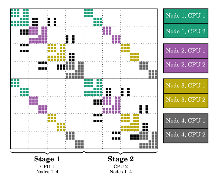
Figure 1: Stage-parallel partitioning of the matrix $\bm{B}=\bm{A}^{-1}\otimes\bm{M}-\Delta t\left(\begin{smallmatrix}\bm{J}_{1}&0\\ 0&\bm{J}_{2}\\ \end{smallmatrix}\right)$. The color of the matrix entries indicates the node to which it belongs. The entries in the first block-column all belong to the first CPU of each node, and the entries the second block-column all belong to the second CPU of each node.

In the context of hybrid shared-distributed memory systems, it is possible to further reduce the communication cost of the stage-parallel IRK algorithm. On such a system, groups of compute cores called nodes have access to the same shared memory. As a consequence, intranode communication is much faster than internode communication. If each stage-group of $s$ processes described above is located on one node, and none of the groups are split across nodes, then the solutions are only communicated within a node, resulting in negligible internode communication costs. An illustration of such an arrangement is shown in Figure 1. The example shown is a scalar problem on a mesh with eight elements, decomposed into four partitions. The hypothetical architecture consists of four compute nodes, each with two CPUs with shared memory. For a two-stage IRK method, each partition of the mesh belongs to a different node, and each of the stages for a given partition belong to different CPUs within one node.

5 Numerical results

5.1 Euler vortex

We solve the compressible Euler equations of gas dynamics, which are given by equations (1) through (3), with the second-order terms removed. The equation of state is given by (5).

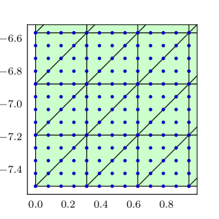
(a) Bottom-left corner of mesh, with $p=4$ DG nodes

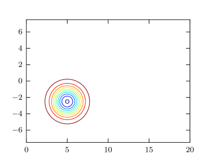
(b) Density contours for the initial conditions

Figure 2: Compressible Euler vortex

We consider the model problem of an unsteady compressible vortex in a rectangular domain [30]. The domain is taken to be the rectangle $[0,20]\times[-7.5,7.5]$, and the vortex is initially centered at $(x_{0},y_{0})=(5,-2.5)$. The vortex is moving with the free-stream at an angle of $\theta$. This problem is particularly useful as a benchmark because the exact solution is given by the following analytic formulas, allowing for convenient computation of the numerical accuracy. The exact solution at $(x,y,t)$ is given by

$$u=u_{\infty}\left(\cos(\theta)-\frac{\epsilon((y-y_{0})-\overline{v}t)}{2\pi r_{c}}\exp\left(\frac{f(x,y,t)}{2}\right)\right),$$ (19)

$$u=u_{\infty}\left(\sin(\theta)-\frac{\epsilon((x-x_{0})-\overline{u}t)}{2\pi r_{c}}\exp\left(\frac{f(x,y,t)}{2}\right)\right),$$ (20)

$$\rho=\rho_{\infty}\left(1-\frac{\epsilon^{2}(\gamma-1)M^{2}_{\infty}}{8\pi^{2}}\exp((f(x,y,t))\right)^{\frac{1}{\gamma-1}},$$ (21)

$$p=p_{\infty}\left(1-\frac{\epsilon^{2}(\gamma-1)M^{2}_{\infty}}{8\pi^{2}}\exp((f(x,y,t))\right)^{\frac{\gamma}{\gamma-1}},$$ (22)

where $f(x,y,t)=(1-((x-x_{0})-\overline{u}t)^{2}-((y-y_{0})-\overline{v}t)^{2})/r_{c}^{2}$, $M_{\infty}$ is the Mach number, $u_{\infty},\rho_{\infty},$ and $p_{\infty}$ are the free-stream velocity, density, and pressure, respectively. The free-stream velocity is given by $(\overline{u},\overline{v})=u_{\infty}(\cos(\theta),\sin(\theta))$. The strength of the vortex is given by $\epsilon$, and its size is $r_{c}$.

For our test case, we choose parameters $\epsilon=15$, $r_{c}=1.5$, $M_{0}=0.5$, $\theta=\arctan(1/2)$. In order for the temporal error to dominate the spatial error, we compute the solution on a fine mesh consisting of 6144 regular right-triangular elements depicted in Figure 2(a). The finite element space is chosen to be piecewise polynomials of degree 4, corresponding to 15 nodes per element. The solution consists of four components, for a total of 368,640 degrees of freedom. The initial conditions are shown in Figure 2(b).

5.1.1 Comparison of preconditioners

We first use this test case to compare the effectiveness of the preconditioners discussed in Section 4.3. As a baseline, we will consider the DIRK solver using the block ILU(0) preconditioner. We will then compare the stage-coupled block ILU(0) and both shifted and unshifted stage-uncoupled ILU(0) preconditioners for the IRK solver. In all cases, we require Newton’s method to converge to an infinity-norm tolerance of $10^{-8}$. We compare the number of GMRES iterations required to converge to a relative, preconditioned tolerance of $10^{-5}$. In order to make a fair comparison between the methods, we will compute the number of $n\times n$ matrix-vector multiplications required per iteration of Newton’s method, across all the stages. We will refer to this quantity as the number of equivalent multiplications. For the DIRK methods, this number is equal to the number of GMRES iterations times the number of implicit stages. For the IRK methods, we recall that each multiplication by the large block matrix of the form (17) essentially consists of $s$ $n\times n$ matrix-vector multiplications.

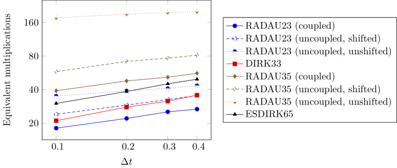
Figure 3: Log-log plot of number of average number of equivalent multiplications vs. $\Delta t$. Coupled preconditioners are shown in solid lines, uncoupled shifted preconditioners in dashed lines, and uncoupled, unshifted preconditioners in dotted lines.

We compute 5 time steps in serial using representative time steps of $\Delta t=0.4,0.3,0.2,$ and $0.1$. We then average the number of GMRES iterations required per linear solve, and multiply this number by the number of implicit stages. For the shifted stage-uncoupled block ILU(0) preconditioner, we choose a shift of $\alpha_{i}=\sum_{j\neq i}\left|A^{-1}_{ji}\right|$, which has in our experience resulted in the fastest convergence. We present the results in the log-log plot shown in Figure 3. We notice that the third order Radau IIA method with the stage-coupled ILU(0) preconditioner requires fewer matrix-vector multiplications than the corresponding third-order DIRK method, while the stage-uncoupled, shifted ILU(0) preconditioner requires roughly the same number of multiplications. For the fifth-order methods, both the coupled and uncoupled preconditioners require more matrix-vector multiplications than the corresponding ESDIRK method. For both third- and fifth-order methods, the stage-uncoupled, unshifted preconditioner requires greatly more matrix-vector multiplications than the other methods, and therefore in the further test cases we will only consider the shifted preconditioner.

5.1.2 Temporal accuracy

Since the analytical solution to this test case is known, it is particularly convenient to compare the accuracy of the time discretization schemes. The solution is integrated until a final time of $t=$60\text{\,}\mathrm{s}$$. For the third-order methods, we choose time steps of $\Delta t=0.4,0.3,0.2,0.1,0.075,0.05,$0.025\text{\,}\mathrm{s}$$. Because of the increased accuracy of the fifth-order methods, we choose larger time steps of $\Delta t=0.8,0.6,0.5,0.4,0.3,$0.2\text{\,}\mathrm{s}$$ for the RADAU35 and ESDIRK65 methods. Time steps between $0.5$ and $1.2\text{\,}\mathrm{s}$ are chosen for the seventh- and ninth-order Radau IIA methods. We approximate the $L^{\infty}$ error by comparing the numerical solution with the known analytic solution at the DG nodes. We also estimate the order of accuracy by comparing successive choices of $\Delta t$ and computing the rate of convergence

$$r_{i}=\frac{\log(L^{\infty}_{i+1}/L^{\infty}_{i})}{\log(\Delta t_{i+1}/\Delta t_{i})},$$

where $L^{\infty}_{i}$ denotes the $L^{\infty}$ error of the numerical solution computed using time step $\Delta t_{i}$. For each method, we present the wall-clock time required to compute the solution in parallel on 16 cores. The results for both the third-order and fifth-order methods are presented in Table 5. The theoretical order of accuracy is observed for all of the methods used. Also listed is the ratio of the DIRK error to the Radau IIA error. Comparing the coefficients presented in Table 1, it can easily be shown that the leading coefficient of the truncation error for the DIRK33 method is about 1.86 times larger than the leading coefficient for the RADAU23 method. We see that the ratio of the errors approaches this value as $\Delta t$ tends to zero. The leading coefficient of the truncation error for the ESDIRK65 methods is about 3.82 times larger than the leading coefficient for the RADAU35 method. In the fifth-order test case, the ratio of the numerical errors is found to be closer to about 1.5, likely because of the additional contribution of spatial discretization error.

Table 5: $L^{\infty}$ error and runtime for the Euler vortex, DIRK and Radau IIA methods (wall-clock time presented for stage-coupled/uncoupled preconditioners).

	RADAU23			DIRK33
$\Delta t$	$L^{\infty}$ error	Order	Time C/UC (s)	$L^{\infty}$ error	Order	Time (s)	Ratio
0.2	$7.2932\times 10^{-2}$	-	820/829	$1.0591\times 10^{-1}$	-	1096	1.452
0.1	$9.7053\times 10^{-3}$	2.91	965/956	$1.6115\times 10^{-2}$	2.72	1268	1.660
0.075	$4.1135\times 10^{-3}$	2.98	1227/1223	$7.1881\times 10^{-3}$	2.81	1618	1.747
0.05	$1.2231\times 10^{-3}$	2.99	1734/1746	$2.2156\times 10^{-3}$	2.90	2291	1.811
0.025	$1.7832\times 10^{-4}$	2.78	3214/3322	$3.0148\times 10^{-4}$	2.88	4212	1.691
	RADAU35			ESDIRK65
$\Delta t$	$L^{\infty}$ error	Order	Time C/UC (s)	$L^{\infty}$ error	Order	Time (s)	Ratio
0.6	$5.8633\times 10^{-2}$	-	843/775	$8.3294\times 10^{-2}$	-	697	1.421
0.5	$2.4239\times 10^{-2}$	4.84	974/810	$3.6075\times 10^{-2}$	4.59	802	1.488
0.4	$7.8902\times 10^{-3}$	5.03	862/905	$1.2605\times 10^{-2}$	4.71	947	1.598
0.3	$1.8156\times 10^{-3}$	5.11	1079/1030	$3.0723\times 10^{-3}$	4.91	1197	1.692
0.2	$2.7294\times 10^{-4}$	4.67	1523/1478	$4.1279\times 10^{-4}$	4.95	1121	1.512

	RADAU47			RADAU59
$\Delta t$	$L^{\infty}$ error	Order	Time C/UC (s)	$\Delta t$	$L^{\infty}$ error	Order	Time C/UC (s)
1.0	$1.8699\times 10^{-2}$	-	1222/1029	1.2	$5.0425\times 10^{-3}$	-	2117/1533
0.8	$4.5413\times 10^{-3}$	6.34	1158/1016	1.0	$1.7294\times 10^{-3}$	5.87	2094/1567
0.6	$8.7259\times 10^{-4}$	5.73	1463/1307	0.8	$4.6966\times 10^{-4}$	5.84	1988/1554
0.5	$3.0265\times 10^{-4}$	5.81	1732/1541	0.6	$8.8679\times 10^{-5}$	5.79	2544/2040

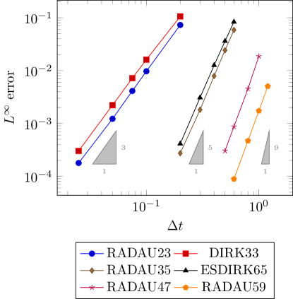
(a) Log-log plot of $L^{\infty}$ error vs. $1/\Delta t$

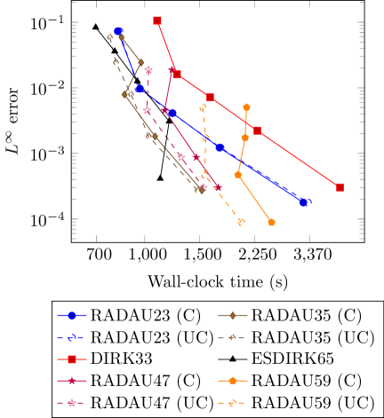
(b) Log-log plot of $L^{\infty}$ error vs. wall-clock time

Figure 4: Log-log plots of $L^{\infty}$ error vs. time-step and wall-clock time for Euler vortex test case. Stage-coupled preconditioners are shown in solid lines, stage-uncoupled in dashed lines.

A log-log plot of the $L^{\infty}$ error vs. $\Delta t$ is shown in Figure 4(a). A log-log plot of the $L^{\infty}$ error vs. wall-clock time is shown in Figure 4(b). We remark that the RADAU23 method achieved the same accuracy as the DIRK33 method in faster runtime for all of the cases considered. Among the fifth-order methods, we did not observe one method to be clearly more efficient than the others. The difference between the stage-coupled and stage-uncoupled preconditioners was found to be insignificant for the third- and fifth-order methods, and the stage-uncoupled preconditioner resulted in faster performance for the seventh- and ninth-order methods.

5.2 High Reynolds number flow over 2D NACA airfoil (LES)

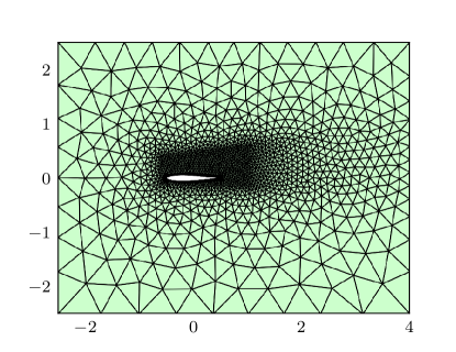
(a) Mesh of NACA airfoil with 3154 elements

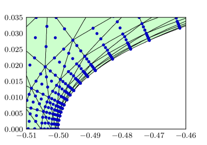
(b) Boundary layer elements with $p=3$ DG nodes

Figure 5: NACA airfoil mesh

In this test case, we consider the two-dimensional viscous flow around a NACA airfoil with an angle of attack of $30\text{\,}\mathrm{\SIUnitSymbolDegree}$. The fluid domain is the rectangle $[-2.5,4]\times[-2.5,2.5]$. For this case, the Mach number is taken to be 0.1, the gas constant 1.4, and the Reynolds number 40,000. The wing is centered vertically, and placed closer to the inlet boundary. The mesh consists of 3154 triangular elements, with finer elements close to the airfoil and in the wake. The mesh and the boundary-layer elements with DG nodes are depicted in Figure 5, and are rotated by $30\text{\,}\mathrm{\SIUnitSymbolDegree}$ to correspond with the desired angle of attack. The triangles near the boundary of the wing are refined in the transverse direction, resulting in highly anisotropic elements. These stretched elements give rise to a highly restrictive CFL condition, suggesting that this problem is particularly well suited to implicit methods. We have found that the CFL condition renders explicit methods impractical for this problem, with the fourth-order explicit Runge-Kutta method exhibiting instability for time steps greater than $7\times 10^{-8}\ $\mathrm{s}$$. On the other hand, the implicit Runge-Kutta methods remain stable for time steps many orders of magnitude larger.

A no-slip condition is enforced on the boundary of the airfoil, and far-field conditions are enforced on all other boundaries. At time $t=$0\text{\,}\mathrm{s}$$ the solution is set to be free-stream everywhere. The solution is then integrated until time $t=$5\text{\,}\mathrm{s}$$, at which point vortices have developed in the wake of the wing. This solution (shown in Figure 6(a)) is taken to be the initial condition for our test case. The finite element space is taken to be piecewise degree 3 polynomials, with 10 nodes per element, resulting in 94,620 degrees of freedom.

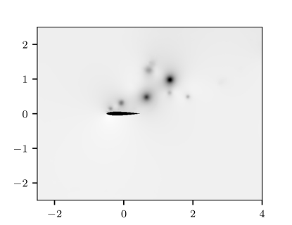
(a) Initial condition, $t=$5\text{\,}\mathrm{s}$$ (density)

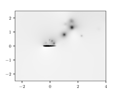
(b) Solution, $t=$5.75\text{\,}\mathrm{s}$$ (density)

Figure 6: Density plots for NACA $\rm Re=40k$ test case

5.2.1 Solver efficiency

We study the effectiveness of the DIRK and Radau IIA IRK methods by comparing both the average number of equivalent multiplications per linear solve and the total wall-clock time. As in the previous case, the methods RADAU23, RADAU35, DIRK33, and ESDIRK65 are used. As in the case of the Euler vortex, a tolerance of $10^{-8}$ is used for the Newton solver. We integrate the equations from time $t=$5\text{\,}\mathrm{s}$$ until $t=$5.75\text{\,}\mathrm{s}$$. For the third-order methods, time steps of $\Delta t=1.25\times 10^{-2},7.50\times 10^{-3},6.25\times 10^{-3},5.00\times 10^{-3},2.50\times 10^{-3},1.25\times 10^{-3},$ are used. For the fifth-order methods, we use the same time steps, in addition to the larger time steps of $\Delta t=5.00\times 10^{-2},$ and $\Delta t=2.50\times 10^{-2}$. In Table 6 we present the runtime and number of equivalent multiplications for all of the methods considered. As in Section 5.1.1, we compute the number of $n\times n$ matrix-vector products performed per Newton iteration (over all the stages) by multiplying the average number of GMRES iterations by the number of implicit stages. In Figure 7(a) we present a log-log plot of the average number of equivalent multiplications vs. $\Delta t$. In Figure 7(b) we present the total wall-clock time required to run the simulation until the final time.

Table 6: Equivalent multiplications and wall-clock time for NACA LES test case

	RADAU23 (Coupled)		RADAU23 (Uncoupled)		DIRK33
$\Delta t$	Mult.	Time (s)	Mult.	Time (s)	Mult.	Time (s)
$1.25\times 10^{-2}$	70.2	75.4	72.0	72.1	100.2	92.1
$7.50\times 10^{-3}$	53.4	96.5	56.0	93.1	81.3	133.0
$6.25\times 10^{-3}$	48.8	105.2	52.4	105.5	73.2	145.7
$5.00\times 10^{-3}$	43.0	116.5	46.2	117.1	65.1	162.9
$2.50\times 10^{-3}$	34.0	208.9	36.8	202.7	42.6	238.0
$1.25\times 10^{-3}$	27.2	389.8	30.8	386.7	33.6	437.5
	RADAU35 (Coupled)		RADAU35 (Uncoupled)		ESDIRK65
$\Delta t$	Mult.	Time (s)	Mult.	Time (s)	Mult.	Time (s)
$5.00\times 10^{-2}$	189.2	59.7	178.5	49.4	216.0	51.3
$2.50\times 10^{-2}$	132.6	79.8	130.2	69.2	173.5	81.0
$1.25\times 10^{-2}$	107.7	141.0	107.1	113.4	137.0	136.6
$7.50\times 10^{-3}$	96.0	189.2	96.0	169.8	107.5	184.6
$6.25\times 10^{-3}$	89.1	222.0	93.3	200.7	95.0	197.2
$5.00\times 10^{-3}$	78.6	230.4	88.8	263.2	81.5	217.8
$2.50\times 10^{-3}$	54.9	340.2	73.5	461.7	60.0	375.9
$1.25\times 10^{-3}$	42.6	619.4	60.6	836.3	47.0	720.1

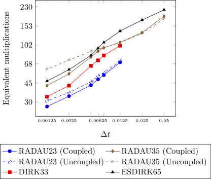
(a) Matrix-vector multiplications vs. $\Delta t$

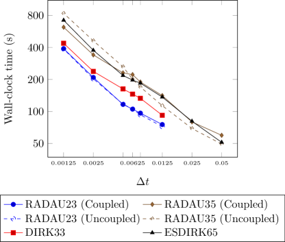
(b) Wall-clock time vs. $\Delta t$

Figure 7: Log-log plots of average number of equivalent multiplications and wall-clock time vs. $\Delta t$ for the 2D NACA LES test case

For the third-order methods, the RADAU23 IRK method required fewer matrix-vector multiplications than the DIRK33 method, for the same choice of $\Delta t$, resulting in a shorter run time. The uncoupled preconditioner resulted in a somewhat larger number of GMRES iterations, and hence more matrix-vector multiplications, but the difference in run time was found to be negligible. For the fifth-order methods, the RADAU35 method with stage-coupled preconditioner resulted in a smaller number of matrix-vector multiplications per linear solve than the ESDIRK65 method. For larger $\Delta t$, the stage-uncoupled preconditioner proved to be effective, resulting in faster run times than both the DIRK method and the stage-coupled preconditioner. For smaller $\Delta t$, the stage-uncoupled preconditioner required a greater number of GMRES iterations and hence longer run times.

5.2.2 Accuracy

Table 7: $L^{\infty}$ error for NACA LES test cases

	RADAU23		DIRK33
$\Delta t$	$L^{\infty}$	Order	$L^{\infty}$	Order	Ratio
$1.25\times 10^{-2}$	$6.006\times 10^{-1}$	-	$4.514\times 10^{-1}$	-	1.668
$7.50\times 10^{-3}$	$1.743\times 10^{-1}$	2.42	$1.615\times 10^{-1}$	2.01	1.706
$6.25\times 10^{-3}$	$1.207\times 10^{-1}$	2.02	$1.423\times 10^{-1}$	0.70	1.717
$5.00\times 10^{-3}$	$8.503\times 10^{-2}$	1.57	$1.216\times 10^{-1}$	0.70	1.735
$2.50\times 10^{-3}$	$1.347\times 10^{-2}$	2.66	$2.022\times 10^{-2}$	2.59	1.839
$1.25\times 10^{-3}$	$1.342\times 10^{-3}$	3.33	$2.708\times 10^{-3}$	2.90	1.823
	RADAU35		ESDIRK65
$\Delta t$	$L^{\infty}$	Order	$L^{\infty}$	Order	Ratio
$5.00\times 10^{-2}$	$4.601\times 10^{-1}$	-	$6.239\times 10^{-1}$	-	2.308
$2.50\times 10^{-2}$	$3.158\times 10^{-1}$	0.54	$5.853\times 10^{-1}$	0.092	1.896
$1.25\times 10^{-2}$	$6.739\times 10^{-2}$	2.23	$1.127\times 10^{-1}$	2.377	2.414
$7.50\times 10^{-3}$	$5.124\times 10^{-3}$	5.04	$3.989\times 10^{-3}$	6.540	4.441
$6.25\times 10^{-3}$	$5.329\times 10^{-3}$	-0.22	$2.147\times 10^{-3}$	3.397	3.263
$5.00\times 10^{-3}$	$2.616\times 10^{-3}$	3.19	$3.279\times 10^{-3}$	-1.897	3.200
$2.50\times 10^{-3}$	$8.135\times 10^{-4}$	1.68	$2.222\times 10^{-3}$	0.561	1.044
$1.25\times 10^{-3}$	$2.059\times 10^{-4}$	1.98	$1.727\times 10^{-4}$	3.686	0.896

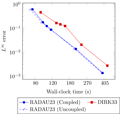
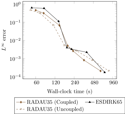
Figure 8: Log-log plots of $L^{\infty}$ errors vs. wall-clock time for the NACA LES test case

We note that the above comparisons were made for equal choices of $\Delta t$. Because the Radau IIA method enjoy a smaller leading coefficient of the truncation error, we expect to achieve better accuracy for the same time step. We therefore study the accuracy of the methods applied to the above problem by considering the semidiscrete system of equations purely as a system of ODEs. We compute a reference solution by numerically integrating the equations for 6000 time steps with $\Delta t=1.25\times 10^{-4}$ using the fifth-order ESDIRK method. Then, we take this solution to be the “exact” solution, with respect to which the $L^{\infty}$ norm of the error is computed, and perform a grid convergence study. For each choice of time step, we compute the $L^{\infty}$ norm of the error, the approximate rate of convergence of the method, and the ratio of the DIRK error to the Radau IIA error in Table 7. In Figure 8, we present log-log plots of the wall-clock time vs. $L^{\infty}$ error. We note that we do not observe the formal order of temporal accuracy for this test problem, possibly due to the choice of time step, which is about five orders of magnitude larger than the explicit CFL, together with the stiff and turbulent nature of the problem. In order to verify the formal order of accuracy, we also run this test problem with time steps that are two to three orders of magnitude smaller than those of the above comparison (for a shorted total time of integration). The results presented in Table 8 confirm that the expected theoretical orders of accuracy are attained for all methods considered.

Table 8: $L^{\infty}$ error for NACA LES test cases (order verification)

	RADAU23		DIRK33
$\Delta t$	$L^{\infty}$	Order	$L^{\infty}$	Order
$6.25\times 10^{-5}$	$5.694\times 10^{-6}$	-	$3.580\times 10^{-6}$	-
$3.125\times 10^{-5}$	$8.765\times 10^{-7}$	2.70	$5.004\times 10^{-7}$	2.84
$1.5625\times 10^{-5}$	$1.177\times 10^{-7}$	2.90	$6.401\times 10^{-8}$	2.97
$7.8125\times 10^{-6}$	$1.494\times 10^{-8}$	2.98	$8.033\times 10^{-9}$	2.99
	RADAU35		ESDIRK65
$\Delta t$	$L^{\infty}$	Order	$L^{\infty}$	Order
$1.25\times 10^{-4}$	$3.438\times 10^{-6}$	-	$1.231\times 10^{-6}$	-
$6.25\times 10^{-5}$	$1.621\times 10^{-7}$	4.41	$4.758\times 10^{-8}$	4.69
$3.125\times 10^{-5}$	$5.434\times 10^{-9}$	4.90	$1.602\times 10^{-9}$	4.89
$1.5625\times 10^{-5}$	$1.964\times 10^{-10}$	4.79	$7.913\times 10^{-11}$	4.34

We remark that for the third-order methods, we can achieve the same accuracy as the DIRK33 method with a faster run time using the RADAU23 method, with both the stage-coupled or stage-uncoupled preconditioner. The differences in run time between the two preconditioners were negligible. For the fifth-order methods, our results indicate that the RADAU35 method outperformed the ESDIRK for a majority of the test cases considered. For this test problem, we found the stage-uncoupled preconditioner to perform better for the larger choices of $\Delta t$.

5.2.3 Parallel performance on NACA airfoil

We study the parallel performance of the IRK and DIRK solvers applied to the two-dimensional NACA airfoil. We choose a representative time step of $\Delta t=1.25\times 10^{-2}$, and integrate the system for five time steps until $t=$5.0625\text{\,}\mathrm{s}$$, using as before the solution at $t=$5\text{\,}\mathrm{s}$$ as the initial condition. We perform this test using both the Radau IIA IRK and the DIRK solvers. For the Radau methods, we use both the stage-coupled and stage-uncoupled ILU(0) preconditioners.

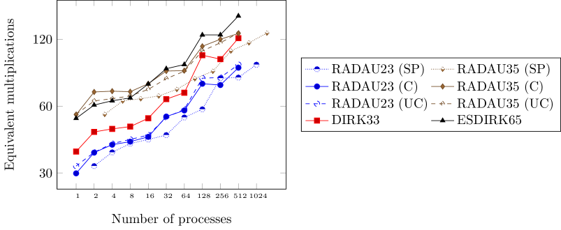
Figure 9: Log-log plot of average number of equivalent multiplications vs. number of processes. Dashed lines indicate stage-uncoupled block ILU(0) preconditioner, and dotted lines indicate stage-parallel solver.

Using the method described in Section 4.5, we decompose the domain into a set number of partitions according to the number of processes. For the DIRK and stage-coupled IRK solvers, the number of partitions is equal to the number of processes. For the stage-uncoupled IRK solver, we can choose the number of partitions to be a factor of $s$ smaller than the number of processes. We consider the mesh decomposed into 1, 2, 4, 8, 16, 32, 64, 128, 256, and 512 partitions. Then, we compute the average number of GMRES iterations required per solve. In the case of the DIRK methods, we multiply the number of iterations by the number of implicit stages to obtain the number of equivalent multiplications performed assuming one Newton iteration. Similarly, in the case of the Radau IIA IRK methods, we multiply the number of iterations by the number of stages to obtain the number of $n\times n$ matrix-vector multiplications. In Figure 9 we show a log-log plot of the average number of equivalent multiplications vs. number of processes.

As the number of processes (and hence number of mesh partitions) increases, we observe an increase in the number of GMRES iterations required to converge. This is because the contributions between different mesh partitions are ignored in the block ILU(0) factorization, rendering the preconditioner less effective. Since the stage-uncoupled ILU(0) preconditioner can be parallelized for the same number of processes with a factor of $s$ fewer partitions, we notice that approximately 15–20% fewer matrix-vector multiplications are required when compared with the standard uncoupled solver. This suggests a substantial benefit to the stage-uncoupled block ILU(0) preconditioner when run in a massively-parallel environment. This difference in performance is numerically validated in the following three-dimensional NACA test case.

5.3 Parallel large eddy simulation (LES) of 3D NACA airfoil

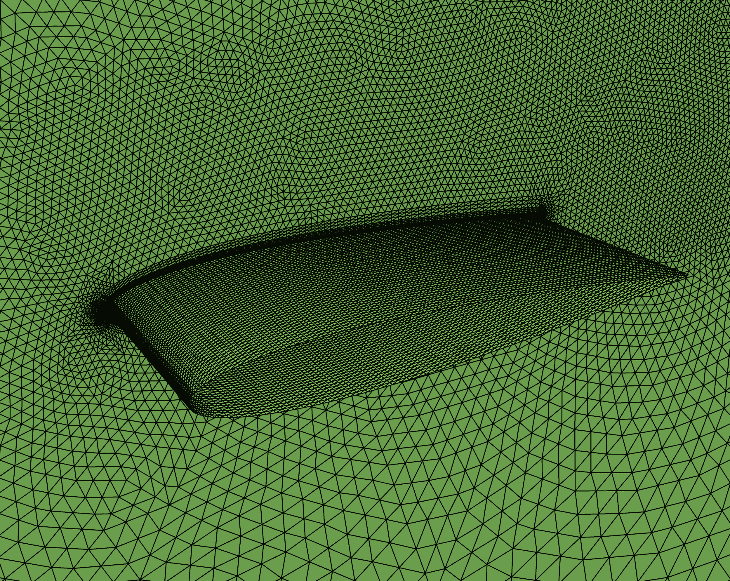
(a) Boundaries of three-dimensional NACA mesh.

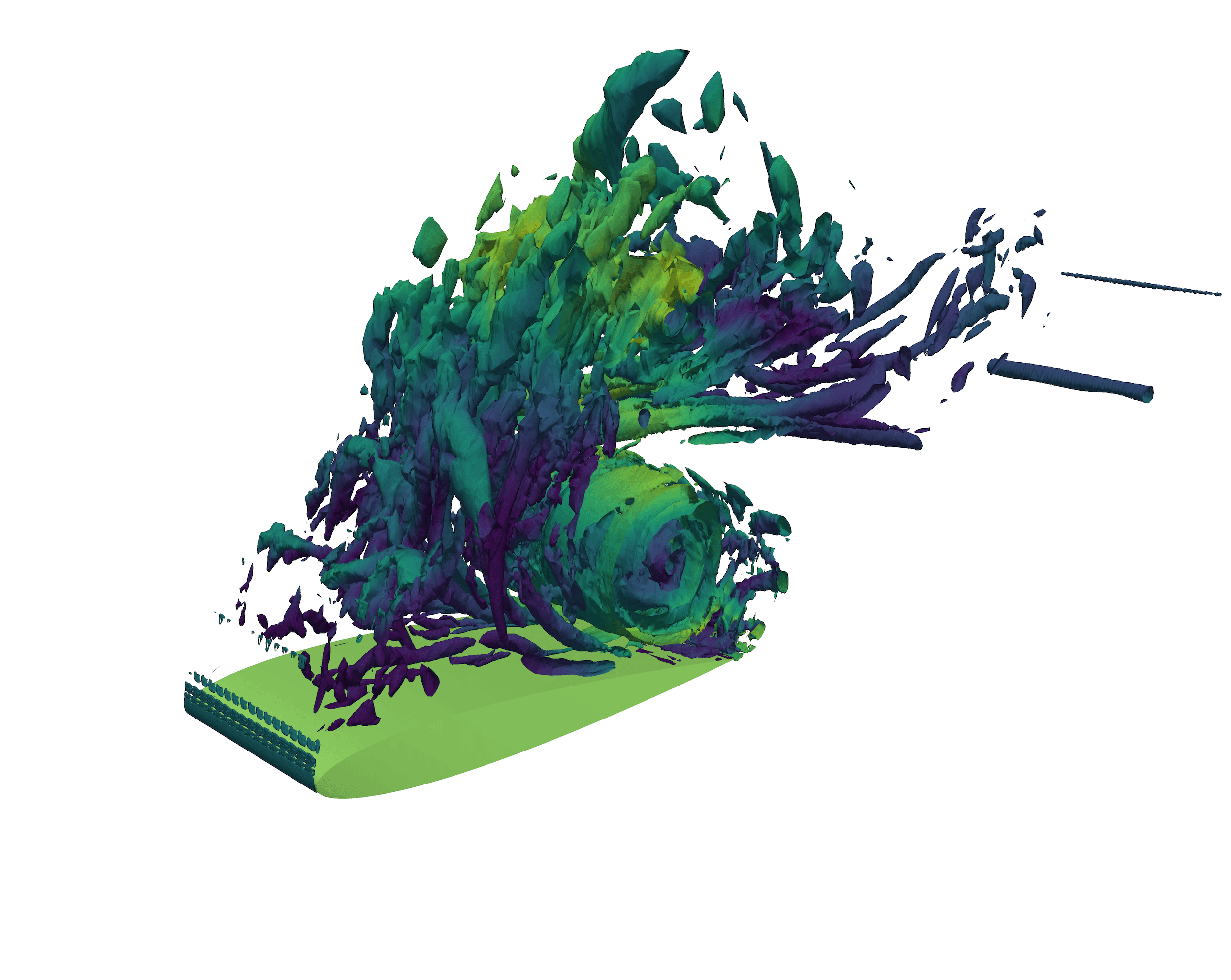
(b) Isosurfaces of $Q$-criterion, $Q=25$, colored by velocity magnitude.

Figure 10: Three-dimensional NACA LES test case.

For our final test case, we consider the three-dimensional viscous flow over a NACA airfoil with angle of attack of $30\text{\,}\mathrm{\SIUnitSymbolDegree}$. The Reynolds number is taken to be 5,300 and the Mach number 0.1. The governing equations are given by equations (1) through (3) with the isentropic assumption discussed in Section 2. The mesh consists of 151,392 tetrahedral elements. The local basis consists of degree 3 polynomials, for a total of 20 nodes per element. We consider the fluid to be isentropic, and hence the solution consists of 4 components, resulting in a total of 12,111,360 degrees of freedom. The mesh is shown in Figure 10(a).

A no-slip condition is enforced on the boundary of the airfoil, periodic conditions are enforced in the span-wise direction, and far-field conditions are enforced on all other boundaries. The solution is initialized to freestream conditions, and then integrated numerically until time $t=$4\text{\,}\mathrm{s}$$ using $\Delta t=$0.02\text{\,}\mathrm{s}$$. At this point, vortices have developed in the wake of the wing. In Figure 10(b), isosurfaces of the $Q$-criterion, for $Q=25$, are shown. The $Q$-criterion, proposed by Dubief and Delcayre in [12] is often used to identify vortical structures, and is defined as the difference of the symmetric and antisymmetric components of the velocity gradient,

$$Q=\frac{1}{2}\left(\Omega_{ij}\Omega_{ij}-S_{ij}S_{ij}\right),$$ (23)

where $\Omega_{ij}=\frac{1}{2}\left(u_{i,j}-u_{j,i}\right)$, and $S_{ij}=\frac{1}{2}\left(u_{i,j}+u_{j,i}\right)$.

We then integrate the equations for 30 time steps using the third- and fifth-order DIRK methods, as well as the Radau IIA methods of order 3, 5, 7, and 9. Due to the turbulent nature of this problem, we do not study the accuracy of the numerical solutions, but rather the efficiency of the solvers for fixed $\Delta t$. We also consider the parallel scaling of the solvers by running our test case on 360, 540, 720, and 1080 processes. For the Radau IIA methods, we consider three preconditioners: stage-coupled, stage-uncoupled, and stage-parallel. As with the DIRK methods, for the stage-coupled and stage-uncoupled preconditioners we decompose the mesh into a number of partitions equal to the number of processes. For the stage-parallel ILU(0) preconditioner we decompose the mesh into a factor of $s$ fewer partitions. The preconditioner then exploits the stage parallelism using the methodology described in Section 4.5. We record the average wall-clock time required per linear solve using each of the methods, and present the results in Figure 11.

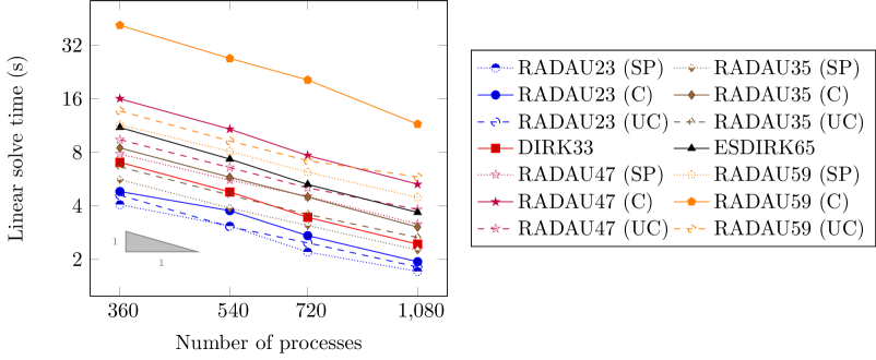
Figure 11: Log-log plot of linear solve time in seconds vs. number of processes. Dashed lines indicate stage-uncoupled block ILU(0) preconditioner, and dotted lines indicate stage-parallel solver. A reference triangle for perfect speedup is shown.

For each order of accuracy, the Radau IIA method with the stage-parallel preconditioner resulted in the fastest runtime. For orders three and five, for which we compare against equal-order DIRK methods, the Radau IIA methods resulted in faster performance with all of the preconditioners considered. Since the number of stages is greater for the higher order methods, and the stage-parallel preconditioner allows for a factor of $s$ fewer mesh partitions, we would expect that the reduction in the number of GMRES iterations due to the improved ILU preconditioner would be greater than for the lower order methods. Indeed, we observe that the relative performance gain of the stage-parallel preconditioner compared with the stage-uncoupled preconditioner increases as the the order of the method increases. For example, while the third-order, stage-parallel preconditioner is only about 5–10% faster than the stage-uncoupled preconditioner, and about 20% faster than the stage-coupled preconditioner, the ninth-order stage-parallel preconditioner is between 20–30% faster than the stage-uncoupled preconditioner, and approximately twice as fast as the stage-coupled preconditioner. Furthermore, as the number of processes approaches the strong scaling limit, we anticipate that the additional factor of $s$ processes allowed by the stage-parallel preconditioner will result in even greater benefit, especially for those methods with a large number of stages.

6 Conclusion

In this paper, we have developed a new strategy for efficiently solving the large, coupled linear systems arising from fully implicit Runge-Kutta time discretizations. By transforming the system of equations, the computational work required per GMRES iterations is reduced significantly. This new method makes it feasible to use high-order, $L$-stable implicit Runge-Kutta methods, such as the Radau IIA methods, as time integrators for discontinuous Galerkin discretizations. We additionally develop new preconditioners for these methods, included a parallel-in-time ILU preconditioner that allows for the computation of the Runge-Kutta stages simultaneously.

Numerical experiments on both two- and three-dimensional fluid flow problems are performed using the Radau IIA methods of up to ninth order. These results indicate that using the transformed system of equations, the fully implicit IRK methods are competitive with, and in our experience, often preferable to the more standard DIRK methods, both in terms of efficiency and accuracy. In a parallel computing environment, the stage-parallel ILU preconditioner results in additional performance gains.

7 Acknowledgments

This research used resources of the National Energy Research Scientific Computing Center, a DOE Office of Science User Facility supported by the Office of Science of the U.S. Department of Energy under Contract No. DE-AC02-05CH11231. The first author was supported by the Department of Defense through the National Defense Science & Engineering Graduate Fellowship Program.

Appendix A Butcher tableaux

RADAU23:	$\begin{aligned} \begin{array}[]{r|rr}1/3&5/12&-1/12\\ 1&3/4&1/4\\ \hline\cr&3/4&1/4\end{array}\end{aligned}$	RADAU35:	$\begin{aligned} \begin{array}[]{r|rrr}\tfrac{2}{5}-\tfrac{\sqrt{6}}{10}&\tfrac{11}{45}-\tfrac{7\sqrt{6}}{360}&\tfrac{37}{225}-\tfrac{169\sqrt{6}}{1800}&-\tfrac{2}{225}+\tfrac{\sqrt{6}}{75}\\ \tfrac{2}{5}+\tfrac{\sqrt{6}}{10}&\tfrac{37}{225}-\tfrac{169\sqrt{6}}{1800}&\tfrac{11}{45}-\tfrac{7\sqrt{6}}{360}&-\tfrac{2}{225}-\tfrac{\sqrt{6}}{75}\\ 1&\tfrac{4}{9}-\tfrac{\sqrt{6}}{36}&\tfrac{4}{9}+\tfrac{\sqrt{6}}{36}&\tfrac{1}{9}\vphantom{\dfrac{1}{2}}\\ \hline\cr&\tfrac{4}{9}-\tfrac{\sqrt{6}}{36}&\tfrac{4}{9}+\tfrac{\sqrt{6}}{36}&\tfrac{1}{9}\end{array}\end{aligned}$
The remaining Radau IIA (4 and 5 stage) tableaux were generated using the following Mathematica code, according to the derivation in [2], where c[n], and A[n] give the abscissa, and Butcher matrix, respectively, for the $n$-stage Radau IIA method. ⬇ 1 q[n_, x_] = LegendreP[n, 2 x - 1] - LegendreP[n - 1, 2 x - 1]; Define the polynomial $Q_{n}(x)$ according to equation (2.1) from [2] 2 c[n_] := (x /. NSolve[q[n, x] == 0, x]) // Re // (Sort[#, Less] &) The abscissa $c_{k}$ are given by the zeros of $Q_{n}(x)$ 3 $\ell$[n_, k_, x_] := q[n, x]/((x - c[n][[k]]) (D[q[n, x], x] /. x -> c[n][[k]])) Define $\ell_{k}(x)$ as in [2] 4 a[n_, i_, k_] := NIntegrate[$\ell$[n, k, x], {x, 0, c[n][[i]]}] The quadrature coefficients $a_{ik}$ are computed as $\int_{0}^{c_{i}}\ell_{k}(x)~{}dx$ 5 A[n_] := Table[a[n, i, k], {i, 1, n}, {k, 1, n}] Finally, we form the Butcher matrix $A$
DIRK33:	$\begin{aligned} \begin{array}[]{r|rrr}\alpha&\alpha&0&0\\ \tau_{2}&\tau_{2}-\alpha&\alpha&0\\ 1&b_{1}&b_{2}&\alpha\\ \hline\cr&b_{1}&b_{2}&\alpha\end{array}\hskip 72.26999pt\begin{array}[]{l}\alpha=1+\frac{\sqrt{6}}{2}\sin\left(\frac{1}{3}\arctan\left(\frac{\sqrt{2}}{4}\right)\right)-\frac{\sqrt{2}}{2}\cos\left(\frac{1}{3}\arctan\left(\frac{\sqrt{2}}{4}\right)\right)\\ \tau_{2}=(1+\alpha)/2\\ b_{1}=-(6\alpha^{2}-16\alpha+1)/4\\ b_{2}=(6\alpha^{2}-20\alpha+5)/4\end{array}\end{aligned}$
ESDIRK65:	$\begin{aligned} \footnotesize\begin{array}[]{r|rrrrrr}0&0&0&0&0&0&0\\ 0.556107682272893&0.2780538411364465&0.2780538411364465&0&0&0&0\\ 1.028127096688746&0.3137405401502951&0.4363327154020044&0.2780538411364465&0&0&0\\ 0.540645375074761&0.2741986534107860&-0.0164268277321164&0.0048197082596452&0.2780538411364465&0&0\\ 0.058741042826253&-0.2441776975175844&-3.3203529439447852&0.0477747285706825&3.2974431145814931&0.2780538411364465&0\\ 1&-0.2786732780227907&1.8929947094010862&-0.1280948204262490&-1.3574693381380240&0.5931888860495311&0.2780538411364465\\ \hline\cr&-0.2786732780227907&1.8929947094010862&-0.1280948204262490&-1.3574693381380240&0.5931888860495311&0.2780538411364465\end{array}\end{aligned}$

References

- [1] Roger Alexander. Diagonally implicit Runge-Kutta methods for stiff O.D.E.’s. SIAM Journal on Numerical Analysis, 14(6):1006–1021, 1977.
- [2] Owe Axelsson. A class of -stable methods. BIT Numerical Mathematics, 9(3):185–199, 1969.
- [3] F. Bassi, L. Botti, A. Colombo, A. Ghidoni, and F. Massa. Linearly implicit Rosenbrock-type Runge-Kutta schemes applied to the discontinuous Galerkin solution of compressible and incompressible unsteady flows. Computers & Fluids, 118:305–320, 2015.
- [4] Hester Bijl, Mark H. Carpenter, Veer N. Vatsa, and Christopher A. Kennedy. Implicit time integration schemes for the unsteady compressible Navier-Stokes equations: Laminar flow. Journal of Computational Physics, 179(1):313–329, 2002.
- [5] Pieter D. Boom and David W. Zingg. High-order implicit temporal integration for unsteady compressible fluid flow simulation. In 21st AIAA Computational Fluid Dynamics Conference. American Institute of Aeronautics and Astronautics (AIAA), 2013.
- [6] Kevin Burrage, Craig Eldershaw, Roger Sidje, et al. A parallel matrix-free implementation of a Runge-Kutta code. In Joint Australian-Taiwanese Workshop on Analysis and Applications, pages 83–88. Centre for Mathematics and its Applications, Mathematical Sciences Institute, The Australian National University, 1999.
- [7] J. C. Butcher. On the implementation of implicit Runge-Kutta methods. BIT Numerical Mathematics, 16(3):237–240, 1976.
- [8] M. H. Carpenter, C. A. Kennedy, Hester Bijl, S. A. Viken, and Veer N. Vatsa. Fourth-order Runge-Kutta schemes for fluid mechanics applications. Journal of Scientific Computing, 25(1):157–194, 2005.
- [9] Mark H. Carpenter, Sally A. Viken, and Eric J. Nielsen. The efficiency of high order temporal schemes. AIAA Paper, 86:2003, 2003.
- [10] Germund G. Dahlquist. A special stability problem for linear multistep methods. BIT Numerical Mathematics, 3(1):27–43, 1963.
- [11] Jacques JB De Swart, Walter M Lioen, and Wolter A Van Der Veen. Specification of PSIDE. Stichting Mathematisch Centrum, 1998.
- [12] Yves Dubief and Franck Delcayre. On coherent-vortex identification in turbulence. Journal of Turbulence, 1(1):011–011, 2000.
- [13] Reinhard Frank, Josef Schneid, and Christoph W Ueberhuber. Order Results for Implicit Runge–Kutta Methods Applied to Stiff Systems. SIAM Journal on Numerical Analysis, 22(3):515–534, 1985.
- [14] Ernst Hairer and Gerhard Wanner. B-Convergence. In Solving Ordinary Differential Equations II, pages 225–238. Springer Berlin Heidelberg, Berlin, Heidelberg, 1996.
- [15] Ernst Hairer and Gerhard Wanner. Construction of Implicit Runge-Kutta Methods. In Solving Ordinary Differential Equations II, pages 71–90. Springer Berlin Heidelberg, Berlin, Heidelberg, 1996.
- [16] Laurent O. Jay and Thierry Braconnier. A parallelizable preconditioner for the iterative solution of implicit Runge–Kutta-type methods. Journal of Computational and Applied Mathematics, 111(1–2):63 – 76, 1999.
- [17] Samuel Kanner and Per-Olof Persson. Validation of a high-order large-eddy simulation solver using a vertical-axis wind turbine. AIAA Journal, 54(1):101–112, 2015.
- [18] A. Kværnø. Singly diagonally implicit Runge-Kutta methods with an explicit first stage. BIT Numerical Mathematics, 44(3):489–502, 2004.
- [19] J. D. Lambert. Numerical methods for ordinary differential systems. John Wiley & Sons, Ltd., Chichester, 1991.
- [20] Thomas A Manteuffel. An incomplete factorization technique for positive definite linear systems. Mathematics of Computation, 34(150):473–497, 1980.
- [21] A. Nigro, A. Ghidoni, S. Rebay, and F. Bassi. Modified extended BDF scheme for the discontinuous Galerkin solution of unsteady compressible flows. International Journal for Numerical Methods in Fluids, 76(9):549–574, 2014.
- [22] Alessandra Nigro, Carmine De Bartolo, Francesco Bassi, and Antonio Ghidoni. Up to sixth-order accurate -stable implicit schemes applied to the discontinuous Galerkin discretized Navier–Stokes equations. Journal of Computational Physics, 276:136 – 162, 2014.
- [23] Jaime Peraire and Per-Olof Persson. The compact discontinuous Galerkin (CDG) method for elliptic problems. SIAM Journal on Scientific Computing, 30(4):1806–1824, 2008.
- [24] Jaime Peraire and Per-Olof Persson. High-order discontinuous Galerkin methods for CFD. In Z. J. Wang, editor, Adaptive High-Order Methods in Fluid Dynamics, chapter 5, pages 119–152. World Scientific, 2011.
- [25] Per-Olof Persson. Scalable parallel Newton-Krylov solvers for discontinuous Galerkin discretizations. In Proceedings of the 47th AIAA Aerospace Sciences Meeting and Exhibit, 2009.
- [26] Per-Olof Persson. High-order LES simulations using implicit-explicit Runge-Kutta schemes. In Proceedings of the 49th AIAA Aerospace Sciences Meeting and Exhibit, AIAA, volume 684, 2011.
- [27] Per-Olof Persson and Jaime Peraire. An efficient low memory implicit DG algorithm for time dependent problems. AIAA paper, 113:2006, 2006.
- [28] Per-Olof Persson and Jaime Peraire. Newton-GMRES preconditioning for discontinuous Galerkin discretizations of the Navier-Stokes equations. SIAM Journal on Scientific Computing, 30(6):2709–2733, 2008.
- [29] W. H. Reed and T. R. Hill. Triangular mesh methods for the neutron transport equation. Los Alamos Report LA-UR-73-479, 1973.
- [30] Z. J. Wang, Krzysztof Fidkowski, Rémi Abgrall, Francesco Bassi, Doru Caraeni, Andrew Cary, Herman Deconinck, Ralf Hartmann, Koen Hillewaert, H. T. Huynh, Norbert Kroll, Georg May, Per-Olof Persson, Bram Leer, and Miguel Visbal. High-order CFD methods: current status and perspective. International Journal for Numerical Methods in Fluids, 72(8):811–845, July 2013.