Electromagnetic Form Factors of Excited Nucleons via Parity-Expanded Variational Analysis

Abstract:

Variational analysis techniques in lattice QCD are powerful tools that give access to the excited state spectrum of QCD. At zero momentum, these techniques are well established and can cleanly isolate energy eigenstates of either positive or negative parity. In order to compute the form factors of a single energy eigenstate, we must perform a variational analysis at non-zero momentum. When we do this with baryons, we run into issues with parity mixing, as boosted baryons are not eigenstates of parity. The parity-expanded variational analysis (PEVA) technique is a novel method for ensuring the successful and consistent isolation of boosted baryon eigenstates. This is achieved through a parity expansion of the operator basis used to construct the correlation matrix. World-first calculations of excited state nucleon form factors using this new technique are presented, showing the improvement over conventional methods.

1 Introduction

In order to evaluate the form factors and transition moments of baryon excitations in lattice QCD, it is necessary to isolate these states at finite momentum. Excited baryons have been isolated on the lattice through a combination of parity projection and variational analysis techniques [1, 2, 3, 4, 5, 6, 7, 8, 9]. At zero momentum, these techniques are well established and can isolate the states of interest. However, at non-zero momentum, these techniques are vulnerable to opposite parity contaminations.

To resolve this issue, we developed the Parity-Expanded Variational Analysis (PEVA) technique [10]. By introducing a novel Dirac projector and expanding the operator basis used to construct the correlation matrix, we are able to cleanly isolate states of both parities at finite momentum.

Utilising the PEVA technique, we are able to present here the world’s first lattice QCD calculations of nucleon excited state form factors free from opposite parity contaminations. Specifically, the Sachs electromagnetic form factors of a localised negative parity nucleon excitation are examined. Furthermore, we clearly demonstrate the efficacy of variational analysis techniques at providing access to ground state form factors with extremely good control over excited state effects.

2 Conventional Variational Analysis

We begin by briefly highlighting where opposite parity contaminations enter into conventional variational analysis techniques and motivate the PEVA technique. In these proceedings we use the Pauli representation for Dirac matrices. In order to discuss opposite parity contaminations, we need to be able to categorise states by their parity. However, eigenstates of non-zero momentum are not eigenstates of parity, so we must categorise boosted states by their rest-frame parity.

To perform a conventional variational analysis on spin-1/2 baryons, we take a basis of $n$ conventional baryon operators ${\chi^{i}}$, which couple to states of both parities,

$$\braket{\Omega}{\chi^{i}}{B^{+}}=\lambda^{i}_{B^{+}}\sqrt{\frac{m_{B^{+}}}{E_{B^{+}}}}\,u_{B^{+}}(p,s)\,,\quad\braket{\Omega}{\chi^{i}}{B^{-}}=\lambda^{i}_{B^{-}}\sqrt{\frac{m_{B^{-}}}{E_{B^{-}}}}\,\gamma_{5}\,u_{B^{-}}(p,s)\,,$$

and use this basis to form an $n\times n$ matrix of two-point correlation functions

$$\mathcal{G}^{ij}(\mathbf{p};\,t):=\, \sum_{\mathbf{x}}\mathrm{e}^{\mathrm{i}\mathbf{p}\cdot\mathbf{x}}\,\braket{\Omega}{\chi^{i}(x)\,\smash{\overline{\chi}}\vphantom{\chi}^{j}(0)}{\Omega}\,.$$

This correlation matrix contains states of both parities, so we introduce the ‘parity projector’ $\Gamma_{\!\pm}=\left(\gamma_{4}\pm\mathbb{I}\right)/2$, and take the spinor trace, defining the projected correlation matrix $G^{ij}(\Gamma_{\!\pm};\,\mathbf{p},\,t):=\,\operatorname{tr}\left(\Gamma_{\!\pm}\,\mathcal{G}^{ij}(\mathbf{p},\,t)\right)$. By inserting a complete set of states between the two operators, and noting the use of Euclidean time, we can rewrite this projected correlation matrix as

$$G^{ij}(\Gamma_{\!\pm};\,\mathbf{p},\,t)=\, \sum_{B^{+}}\mathrm{e}^{-E_{B^{+}}(\mathbf{p})\,t}\,\lambda^{i}_{B^{+}}\,\smash{\overline{\lambda}}\vphantom{\lambda}^{j}_{B^{+}}\frac{E_{B^{+}}\!(\mathbf{p})\,\pm m_{B^{+}}}{2E_{B^{+}}\!(\mathbf{p})}+\sum_{B^{-}}\mathrm{e}^{-E_{B^{-}}(\mathbf{p})\,t}\,\lambda^{i}_{B^{-}}\,\smash{\overline{\lambda}}\vphantom{\lambda}^{j}_{B^{-}}\frac{E_{B^{-}}\!(\mathbf{p})\,\mp m_{B^{-}}}{2E_{B^{-}}\!(\mathbf{p})}\,,$$

At zero momentum, $E_{B}(\mathbf{0})=m_{B}$ and the projected correlation matrices will each contain terms of a single parity. However, at non-zero momentum $E_{B}(\mathbf{p})\neq m_{B}$ and the projected correlation matrices contain $O\left((E-m)/2E\right)$ opposite parity contaminations. These opposite parity contaminations were investigated in Ref. [11].

3 Parity-Expanded Variational Analysis

To solve the problem of opposite parity contaminations at finite momentum, we developed the PEVA technique [10]. In this section, we summarise the PEVA technique, and describe how it applies to form factor calculations.

The PEVA technique works by expanding the operator basis of the correlation matrix to isolate energy eigenstates of both rest-frame parities simultaneously while still retaining a signature of this parity. By considering the Dirac structure of the unprojected correlation matrix, we construct the novel momentum-dependent projector $\Gamma_{\!\mathbf{p}}:=\,\frac{1}{4}\left(\mathbb{I}+\gamma_{4}\right)\left(\mathbb{I}-\mathrm{i}\gamma_{5}\gamma_{k}\hat{\mathbf{p}}_{k}\right)$. This allows us to construct a set of “parity-signature” projected operators $\left\{\chi^{i}_{\mathbf{p}}=\Gamma_{\!\mathbf{p}}\,\chi^{i}\,,\;\chi^{i^{\prime}}_{\mathbf{p}}=\Gamma_{\!\mathbf{p}}\,\gamma_{5}\,\chi^{i}\right\}$, where the primed indices denote the inclusion of $\gamma_{5}$, inverting the way the operators transform under parity. Unlike the conventional opertors ${\,\chi^{i}\,}$, the inclusion of $\Gamma_{\!\mathbf{p}}$ ensures that the operators $\chi^{i}_{\mathbf{p}}$ and $\chi^{i^{\prime}}_{\mathbf{p}}$ have definite parity at zero momentum without requiring projection by $\Gamma_{\pm}$.

By performing a variational analysis with this expanded basis [10], we construct optimised operators $\phi^{\alpha}_{\mathbf{p}}(x)$ that couple to each state $\alpha$. We can then use these operators to calculate the three point correlation function

$$\mathcal{G}^{\mu}_{+}(\mathbf{p^{\prime}},\mathbf{p};\,t_{2},t_{1};\,\alpha):=\, \sum_{\mathbf{x_{2}},\mathbf{x_{1}}}e^{-\mathrm{i}\mathbf{p^{\prime}}\cdot\mathbf{x_{2}}}\,e^{\mathrm{i}(\mathbf{p^{\prime}}-\mathbf{p})\cdot\mathbf{x_{1}}}\braket{\,\phi^{\alpha}_{\mathbf{p^{\prime}}}(x_{2})\,}{\,J^{\mu}(x_{1})\,}{\,\smash{\overline{\phi}}\vphantom{\phi}^{\alpha}_{\mathbf{p}}(0)\,}\,,$$

where $J^{\mu}$ is the $O(a)$-improved [12] conserved vector current used in [13], inserted with some momentum transfer $q=p^{\prime}-p$. We can take the spinor trace of this with some projector $\Gamma$ to get the projected three point correlation function $G^{\mu}_{+}(\mathbf{p^{\prime}},\mathbf{p};\,t_{2},t_{1};\,\Gamma;\,\alpha):=\,\operatorname{tr}\left(\Gamma\,\mathcal{G}^{\mu}_{+}(\mathbf{p^{\prime}},\mathbf{p};\,t_{2},t_{1};\,\alpha)\right)$.

There is an arbitrary sign choice in the definition of $\Gamma_{\!\mathbf{p}}$, so it is convenient to define $\Gamma_{\!\mathbf{p}}^{\prime}:=\,\frac{1}{4}\left(\mathbb{I}+\gamma_{4}\right)\left(\mathbb{I}+\mathrm{i}\gamma_{5}\gamma_{k}\hat{\mathbf{p}}_{k}\right)=\Gamma_{\!\mathbf{-p}}$, which is equally valid. We can then use this alternate projector in constructing an alternate sink operator $\phi^{\prime\alpha}_{\mathbf{p}}(x)$, while leaving the source operator unchanged. This gives us an alternate three point correlation function, $\mathcal{G}^{\mu}_{-}(\mathbf{p^{\prime}},\mathbf{p};\,t_{2},t_{1};\,\alpha)$, leading to an alternate projected three point correlation function, $G^{\mu}_{-}(\mathbf{p^{\prime}},\mathbf{p};\,t_{2},t_{1};\,\Gamma;\,\alpha)$.

We can then construct the reduced ratio,

$$\smash{\overline{R}}\vphantom{R}_{\pm}(\mathbf{p^{\prime}},\mathbf{p};\,\alpha;\,r,s):=\,\, \sqrt{\left|\frac{r_{\mu}\,G^{\mu}_{\pm}(\mathbf{p^{\prime}},\mathbf{p};\,t_{2},t_{1};\,s_{\nu}\,\Gamma_{\!\nu};\,\alpha)\;r_{\rho}\,G^{\rho}_{\pm}(\mathbf{p},\mathbf{p^{\prime}};\,t_{2},t_{1};\,s_{\sigma}\,\Gamma_{\!\sigma};\,\alpha)}{G(\mathbf{p^{\prime}};\,t_{2};\,\alpha)\,G(\mathbf{p};\,t_{2};\,\alpha)}\right|}$$

$$\quad\times\mathrm{sign}\left(r_{\gamma}\,G^{\gamma}_{\pm}(\mathbf{p^{\prime}},\mathbf{p};\,t_{2},t_{1};\,s_{\delta}\,\Gamma_{\delta};\,\alpha)\right)\sqrt{\frac{2E_{\alpha}(\mathbf{p})}{E_{\alpha}(\mathbf{p})+m_{\alpha}}}\,\sqrt{\frac{2E_{\alpha}(\mathbf{p^{\prime}})}{E_{\alpha}(\mathbf{p^{\prime}})+m_{\alpha}}}\,,$$

where $r_{\mu}$ and $s_{\mu}$ are coefficients selected to determine the form factors. By investigating the $r_{\mu}$ and $s_{\mu}$ dependence of $\smash{\overline{R}}\vphantom{R}_{\pm}$, we find that the clearest signals are given by

$$R^{T}_{\pm} =\frac{2}{1\pm\,\hat{\mathbf{p}}\cdot\hat{\mathbf{p^{\prime}}}}\;\smash{\overline{R}}\vphantom{R}_{\pm}\left(\mathbf{p^{\prime}},\mathbf{p};\,\alpha;\,(1,\mathbf{0}),(1,\mathbf{0})\right)\,,\;\mathrm{and}$$

$$R^{S}_{\mp} =\frac{2}{1\pm\,\hat{\mathbf{p}}\cdot\hat{\mathbf{p^{\prime}}}}\;\smash{\overline{R}}\vphantom{R}_{\mp}\left(\mathbf{p^{\prime}},\mathbf{p};\,\alpha;\,(0,\hat{\mathbf{r}}),(0,\hat{\mathbf{s}})\right)\,,$$

where $\hat{\mathbf{s}}$ is chosen such that $\mathbf{p}\cdot\hat{\mathbf{s}}=0=\mathbf{p^{\prime}}\cdot\hat{\mathbf{s}}$, $\hat{\mathbf{r}}$ is equal to $\hat{\mathbf{q}}\times\hat{\mathbf{s}}$, and the sign $\pm$ is chosen such that $1\pm\hat{\mathbf{p}}\cdot\hat{\mathbf{p^{\prime}}}$ is maximised.

We can then find the Sachs electric and magnetic form factors

$$G_{E}(Q^{2})=\, \left[Q^{2}\left(E_{\alpha}(\mathbf{p^{\prime}})+E_{\alpha}(\mathbf{p})\right)\,\left(\left(E_{\alpha}(\mathbf{p})+m_{\alpha}\right)\,\left(E_{\alpha}(\mathbf{p^{\prime}})+m_{\alpha}\right)\mp\bigl{|}\mathbf{p}\bigr{|}\bigl{|}\mathbf{p^{\prime}}\bigr{|}\right)\,R^{T}_{\pm}\right.$$

$$\left.\quad\pm\,2\bigl{|}\mathbf{q}\bigr{|}\left(1\mp\,\hat{\mathbf{p}}\cdot\hat{\mathbf{p^{\prime}}}\right)\bigl{|}\mathbf{p}\bigr{|}\bigl{|}\mathbf{p^{\prime}}\bigr{|}\left(\left(E_{\alpha}(\mathbf{p})+m_{\alpha}\right)\,\left(E_{\alpha}(\mathbf{p^{\prime}})+m_{\alpha}\right)\pm\bigl{|}\mathbf{p}\bigr{|}\bigl{|}\mathbf{p^{\prime}}\bigr{|}\right)\,R^{S}_{\mp}\right]$$

$$/\left[4m_{\alpha}\left[\left(E_{\alpha}(\mathbf{p})\,E_{\alpha}(\mathbf{p^{\prime}})+m_{\alpha}^{2}\mp\,\bigl{|}\mathbf{p}\bigr{|}\bigl{|}\mathbf{p^{\prime}}\bigr{|}\right)\bigl{|}\mathbf{q}\bigr{|}^{2}+4\bigl{|}\mathbf{p}\bigr{|}^{2}\bigl{|}\mathbf{p^{\prime}}\bigr{|}^{2}\left(1\mp\,\hat{\mathbf{p}}\cdot\hat{\mathbf{p^{\prime}}}\right)\right]\right]\,,\;\mathrm{and}$$

$$G_{M}(Q^{2})=\, \left[\pm\,2\left(1\mp\,\hat{\mathbf{p}}\cdot\hat{\mathbf{p^{\prime}}}\right)\bigl{|}\mathbf{p}\bigr{|}\bigl{|}\mathbf{p^{\prime}}\bigr{|}\left(\left(E_{\alpha}(\mathbf{p})+m_{\alpha}\right)\,\left(E_{\alpha}(\mathbf{p^{\prime}})+m_{\alpha}\right)\pm\bigl{|}\mathbf{p}\bigr{|}\bigl{|}\mathbf{p^{\prime}}\bigr{|}\right)\,R^{T}_{\pm}\right.$$

$$\left.\quad-\bigl{|}\mathbf{q}\bigr{|}\left(E_{\alpha}(\mathbf{p^{\prime}})+E_{\alpha}(\mathbf{p})\right)\,\left(\left(E_{\alpha}(\mathbf{p})+m_{\alpha}\right)\,\left(E_{\alpha}(\mathbf{p^{\prime}})+m_{\alpha}\right)\mp\bigl{|}\mathbf{p}\bigr{|}\bigl{|}\mathbf{p^{\prime}}\bigr{|}\right)\,R^{S}_{\mp}\right]$$

$$/\left[2\left[\left(E_{\alpha}(\mathbf{p})\,E_{\alpha}(\mathbf{p^{\prime}})+m_{\alpha}^{2}\mp\,\bigl{|}\mathbf{p}\bigr{|}\bigl{|}\mathbf{p^{\prime}}\bigr{|}\right)\bigl{|}\mathbf{q}\bigr{|}^{2}+4\bigl{|}\mathbf{p}\bigr{|}^{2}\bigl{|}\mathbf{p^{\prime}}\bigr{|}^{2}\left(1\mp\,\hat{\mathbf{p}}\cdot\hat{\mathbf{p^{\prime}}}\right)\right]\right]\,.$$

The details of this procedure will be presented in full in Ref. [14].

4 Results

In this section, we present world-first lattice QCD calculations of the Sachs electric and magnetic form factors of the ground state nucleon and first negative-parity excitation with good control over opposite parity contaminations. We compare the results obtained by the PEVA technique to an analysis using conventional parity projection.

These results are calculated on the second heaviest PACS-CS $(2+1)$-flavour full-QCD ensemble [15], made available through the ILDG [16]. This ensemble uses a $32^{3}\times 64$ lattice, and employs an Iwasaki gauge action with $\beta=1.90$ and non-perturbatively $O(a)$-improved Wilson quarks. We use the $m_{\pi}=$570\text{\,}\mathrm{MeV}$$ PACS-CS ensemble, and set the scale using the Sommer parameter with $r_{0}=$0.49\text{\,}\mathrm{fm}$$, giving a lattice spacing of $a=$0.1009(23)\text{\,}\mathrm{fm}$$. With this scale, our pion mass is $515(8)\text{\,}\mathrm{MeV}$. We used 343 gauge field configurations, with a single source location on each configuration. $\chi^{2}/\mathrm{dof}$ is calculared with the full covariance matrix, and all fits have $\chi^{2}/\mathrm{dof}\ <1.2$.

For the analyses in this section, we start with a basis of eight operators, by taking two conventional spin-$\nicefrac{{1}}{{2}}$ nucleon operators ($\,\chi_{1}=\epsilon^{abc}\,[{u^{a}}^{\top}(C\gamma_{5})\,d^{b}]\,u^{c}$, and $\chi_{2}=\epsilon^{abc}\,[{u^{a}}^{\top}(C)\,d^{b}]\,\gamma_{5}\,u^{c}\,$), and applying 16, 35, 100, and 200 sweeps of gauge invariant Gaussian smearing when creating the propagators [2]. For the conventional variational analysis, we take this basis of eight operators and project with $\Gamma_{\!\pm}$, and for the PEVA analysis, we parity expand the basis to sixteen operators and project with $\Gamma_{\!\mathbf{p}}$ and $\Gamma_{\!\mathbf{p}}^{\prime}$.

To extract the form factors, we fix the source at time slice 16, and the current insertion at time slice 21. We choose time slice 21 by inspecting the two point correlation functions associated with each state and observing that excited state contaminations are strongly suppressed by time slice 21. We then extract the form factors from the ratios given in Sec. 3 for every possible sink time and look for a plateau consistent with a single-state ansatz.

Beginning with the ground state, in Fig. 1 we plot $G_{E}(Q^{2})$ and in Fig. 2 we plot $G_{M}(Q^{2})$ with respect to sink time, at $Q^{2}=$0.144\text{\,}\mathrm{G}\mathrm{eV}^{2}$$. There are only slight differences between the results extracted by PEVA and the results extracted by a conventional variational analysis in this case. We believe this is because the opposite parity contaminations are small, and come from heavier states that are suppressed by Euclidean time evolution.

For both the PEVA and conventional variational analysis, we see very clear and clean plateaus in the form factors, indicating very good control over excited state contaminations. This supports previous work demonstrating the utility of variational analysis in calculating baryon matrix elements [17, 18]. By using such techniques we are able to cleanly isolate precise values for the Sachs electric and magnetic form factors of the ground state nucleon.

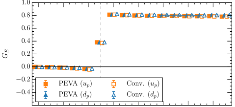
Figure 1: $G_{E}(Q^{2})$ for the ground state nucleon at $Q^{2}=$0.144\text{\,}\mathrm{G}\mathrm{eV}^{2}$$. We plot the conventional analysis with open markers and the new PEVA analysis with closed markers. Our fits to the plateaus are illustrated by shaded bands, with the central value indicated by dashed lines for the conventional analysis, and solid lines for the PEVA analysis. We plot the contributions from the singly represented quark sector with blue triangles, and doubly represented quark sector with orange squares, for single quarks of unit charge.

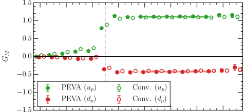
Figure 2: $G_{M}(Q^{2})$ for the ground state nucleon at $Q^{2}=$0.144\text{\,}\mathrm{G}\mathrm{eV}^{2}$$. We plot the conventional analysis with open markers and dashed lines and the PEVA analysis with closed markers and solid lines. The contributions from the singly represented quark sector are plotted with red hexagons, and from the doubly represented quark sector with green pentagons, for single quarks of unit charge.

Moving on to the first negative parity excited state, in Fig. 3 we plot $G_{E}(Q^{2})$ at $Q^{2}=$0.146\text{\,}\mathrm{G}\mathrm{eV}^{2}$$ vs the sink time. We see that the PEVA analysis (closed points) allows us to fit a plateau (shaded bands with solid lines) at a much earlier time, and with a significantly different value to the conventional analysis (open points, dashed lines). This demonstrates the effectiveness of the PEVA technique at removing opposite parity contaminations. The localised nature of this state is manifest in the large values for $G_{E}(Q^{2})$, similar to that for the proton. We also see similar improvements in $G_{M}(Q^{2})$, as presented in Fig. 4.

Figure 3: $G_{E}(Q^{2})$ for the first negative parity excitation of the nucleon at $Q^{2}=$0.146\text{\,}\mathrm{G}\mathrm{eV}^{2}$$. We plot the the conventional analysis with open markers and dashed lines, and the new PEVA analysis with closed markers and solid lines. We plot the contributions from the singly represented quark sector with blue triangles, and doubly represented quark sector with orange squares, for single quarks of unit charge. The PEVA analysis plateaus at a much earlier time with a significantly different value, demonstrating its effectiveness.

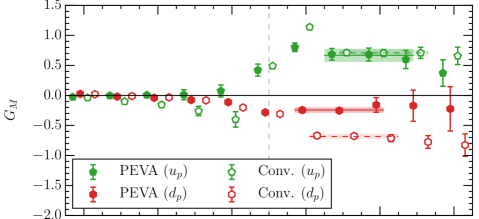
Figure 4: $G_{M}(Q^{2})$ for the ground state nucleon at $Q^{2}=$0.146\text{\,}\mathrm{G}\mathrm{eV}^{2}$$. We plot the conventional analysis with open markers and dashed lines and the PEVA analysis with closed markers and solid lines. The contributions from the singly represented quark sector are plotted with red hexagons, and from the doubly represented quark sector with green pentagons, for single quarks of unit charge. The significantly different values of $G_{M}(Q^{2})$ for the singly represented quark sector demonstrate the importance of the PEVA technique.

5 Conclusion

We have demonstrated the effectiveness of the PEVA technique specifically and variational analysis techniques in general at controlling excited state effects. For the ground state nucleon, conventional variational analysis techniques are sufficient to provide clean plateaus that allow for the effective extraction of form factors. However, for excited states, opposite parity contaminations have a clear and significant effect. The PEVA technique allows us to remove these contaminations and calculate the form factors of excited nucleons for the first time.

References

- [1] A. L. Kiratidis, W. Kamleh, D. B. Leinweber and B. J. Owen, Lattice baryon spectroscopy with multi-particle interpolators, Phys. Rev. D91 (2015) 094509, [1501.07667].
- [2] M. S. Mahbub, W. Kamleh, D. B. Leinweber, P. J. Moran and A. G. Williams, Structure and Flow of the Nucleon Eigenstates in Lattice QCD, Phys.Rev. D87 (2013) 094506, [1302.2987].
- [3] M. S. Mahbub, W. Kamleh, D. B. Leinweber, P. J. Moran and A. G. Williams, Low-lying Odd-parity States of the Nucleon in Lattice QCD, Phys. Rev. D87 (2013) 011501, [1209.0240].
- [4] CSSM Lattice collaboration, M. S. Mahbub, W. Kamleh, D. B. Leinweber, P. J. Moran and A. G. Williams, Roper Resonance in 2+1 Flavor QCD, Phys. Lett. B707 (2012) 389–393, [1011.5724].
- [5] Hadron Spectrum collaboration, R. G. Edwards et al., Flavor structure of the excited baryon spectra from lattice QCD, Phys.Rev. D87 (2013) 054506, [1212.5236].
- [6] R. G. Edwards, J. J. Dudek, D. G. Richards and S. J. Wallace, Excited state baryon spectroscopy from lattice QCD, Phys. Rev. D84 (2011) 074508, [1104.5152].
- [7] C. B. Lang, L. Leskovec, M. Padmanath and S. Prelovsek, Pion-nucleon scattering in the Roper channel from lattice QCD, 1610.01422.
- [8] C. Lang and V. Verduci, Scattering in the negative parity channel in lattice QCD, Phys.Rev. D87 (2013) 054502, [1212.5055].
- [9] C. Alexandrou, T. Leontiou, C. N. Papanicolas and E. Stiliaris, Novel analysis method for excited states in lattice QCD: The nucleon case, Phys. Rev. D91 (2015) 014506, [1411.6765].
- [10] F. M. Stokes et al., Parity-expanded variational analysis for nonzero momentum, Phys. Rev. D92 (2015) 114506, [1302.4152].
- [11] F. X. Lee and D. B. Leinweber, Negative parity baryon spectroscopy, Nucl. Phys. Proc. Suppl. 73 (1999) 258–260, [hep-lat/9809095].
- [12] G. Martinelli, C. T. Sachrajda and A. Vladikas, A Study of ’improvement’ in lattice QCD, Nucl. Phys. B358 (1991) 212–227.
- [13] S. Boinepalli et al., Precision electromagnetic structure of octet baryons in the chiral regime, Phys. Rev. D74 (2006) 093005, [hep-lat/0604022].
- [14] F. M. Stokes, W. Kamleh, D. B. Leinweber and B. J. Owen, in preparation.
- [15] PACS-CS collaboration, S. Aoki et al., 2+1 Flavor Lattice QCD toward the Physical Point, Phys. Rev. D79 (2009) 034503, [0807.1661].
- [16] M. G. Beckett, B. Joo, C. M. Maynard, D. Pleiter, O. Tatebe and T. Yoshie, Building the International Lattice Data Grid, Comput. Phys. Commun. 182 (2011) 1208–1214, [0910.1692].
- [17] J. Dragos et al., Nucleon matrix elements using the variational method in lattice QCD, Phys. Rev. D94 (2016) 074505, [1606.03195].
- [18] B. J. Owen, J. Dragos, W. Kamleh, D. B. Leinweber, M. S. Mahbub, B. J. Menadue et al., Variational Approach to the Calculation of gA, Phys. Lett. B723 (2013) 217–223, [1212.4668].