2012 Vol. X No. XX, 000–000
11institutetext: Department of Astronomy, Beijing Normal University, Beijing 100875,
China; hnwilliam@hotmail.com; bisl@bnu.edu.cn
22institutetext: Department of Astronomy, Peking University, Beijing 100871, China; tianzhijia@pku.edu.cn
33institutetext: Sydney Institute for Astronomy (SIfA), School of Physics, University of Sydney, NSW 2006, Australia;
44institutetext: Stellar Astrophysics Centre, Department of Physics and Astronomy, Aarhus University, Ny Munkegade 120, DK-8000 Aarhus C, Denmark
\vs\no
Seismic diagnostics of solar-like oscillating stars
Abstract
High precision and long-lasting Kepler data enabled us to estimate stellar properties with asteroseismology as an accurate tool. We performed asteroseismic analysis on six solar-like stars observed by the Kepler mission: KIC 6064910, KIC 6766513, KIC 7107778, KIC 10079226, KIC 10147635 and KIC 12069127. The extraction of seismic information includes two parts. First, we obtained two global asteroseismic parameters, mean large separation and frequency of maximum power , with autocorrelation function and collapsed autocorrelation function. Second, we extracted individual oscillation modes with low- degree using a least-squares fit. Stellar grid models were built with Yale Rotating Stellar Evolution Code (YREC) to analyze stellar properties. They covered the range of with a step of 0.02 and with a step of 0.1 . We used a Bayesian approach to estimate stellar fundamental parameters of the six stars, under the constraints of asteroseismic parameters (, ) and non-asteroseismic parameters (, ). We discover that the six targets include five sub-giant stars with and one main-sequence star with , and with ages in the range of .
keywords:
stars: evolution — stars: oscillations — stars: fundamental parameters1 Introduction
Recent space missions, such as CoRoT and Kepler mission, have led us to a golden epoch when large scale asteroseismic analysis of stars can be carried out. Thanks to the high precision and long-lasting observation provided by these space missions, new previously unavailable areas of frequency domain have been opened (e.g. Appourchaux et al. 2008; Borucki et al. 2007; Gilliland et al. 2010; Gruberbauer et al. 2013). With detected oscillation, the following aseteroseismic studies are able to provide us a unique approach to constrain the star’s fundamental properties, and even to test the theory of stellar structure and evolution. They enrich our knowledge not only on stars, but also on clusters and the Galaxy, or even broader, the whole universe (e.g. Soriano et al. 2007; Doǧan et al. 2013; Campante et al. 2015; Casanellas 2015; Sharma et al. 2016).
Solar-like oscillations refer to stars oscillating with the same mechanism as the Sun, where they are stochastically excited and damped by convection motion in the near-surface convection zone (e.g. Christensen-Dalsgaard 1982; Christensen-Dalsgaard & Frandsen 1983; Houdek et al. 1999). Study of oscillations could yield worthful conceptions on stellar structures and evolutionary stages. Main-sequence stars behave as p modes (pressure dominated) in the envelope. Sub-giant stars behave as mixed modes, which are characterized by g modes (gravity dominated) in the core and p modes in the envelope (Tassoul 1980), when “avoided crossing” commence (Aizenman et al. 1977; Benomar et al. 2014; Lagarde et al. 2015). Therefore, oscillations are capable of distinguishing different types of stars with their identical signatures. Mixed modes have further shown potential on constraining stellar models in a powerful way (e.g. Deheuvels et al. 2012; Montalbán & Noels 2013; Silva Aguirre et al. 2013; Mosser et al. 2014; Mosser 2015), since some stellar parameters are particularly sensitive to them, e.g. stellar age (Metcalfe et al. 2010) and mass (Benomar et al. 2012). It is even possible to determine the presence and size of the convective core with the help of asteroseismology (Liu et al. 2014; Yang et al. 2015).
Accurate data analysis on oscillation is one crucial prerequisite for detailed stellar diagnostics (e.g. Ozel et al. 2010; Deheuvels et al. 2012; Silva Aguirre et al. 2013; Silva Aguirre et al. 2014; Chaplin et al. 2014). Two global asteroseismic parameters, mean large separation and frequency of maximum power which reflect the star’s properties, have been designed to extract through pipelines (e.g. Chaplin et al. 2014; Verner et al. 2011; Davies et al. 2016), which is even possible when the signal to noise ratio (S/N) is not that high (e.g. Chaplin et al. 2008, Stello et al. 2009b). Individual oscillation frequencies, which can provide more insights related to a star’s interior, have been broadly analyzed when convolved with maximum likelihood estimators and Bayesian estimators (e.g. Davies et al. 2016; Appourchaux et al. 2014; Appourchaux et al. 2012). In this work, we aim to analyze a low-mass sample of main-sequence stars and sub-giant stars by deriving , , and individual oscillation frequencies. This approach is expected to detect low angular degree (e.g. ) modes while modes with higher angular degree remain invisible due to geometrical cancellation. With global seismic parameters, deriving stellar properties would be an obvious and simple way to investigate these stars.
The article is organized as follows. In section 2, we briefly introduce our selection of targets. In section 3, we illustrate the process of derivation of two seismic parameters and , and individual oscillation frequencies. In section 4, we present stellar model construction and their usage in estimating stellar fundamental parameters of the six stars. Finally, discussions and conclusions are shown in section 5.
2 List of targets
We revisited the topic explored by Chaplin et al. (2014), who derived the values of mean large separation and frequency of maximum power . We selected six targets which met the following criteria: S/N values are high enough to obtain individual oscillation frequencies, and they have not been extracted in any work before. We intend to obtain and in our own way to test if our method works well, and then derive oscillation frequencies with which detailed asteroseismic diagnostics could be realized.
The Kepler mission provides photometric time series of the targets with long cadence (LC; 29.43 min sampling) and short cadence (SC; 58.84s sampling). The pulsation frequency range is estimated to be above the Nyquist frequency of LC data. Here, we obtained SC time series over one year, which were collected from the Kepler Asteroseismic Science Consortium website111http://kasoc.phys.au.dk/. They had been preprocessed by the Kepler Working Group (WG#1, García et al. 2011). Table 1 shows Kepler mission data we used in this work.
Atmospheric parameters of the stars are crucial since they serve as constraints on stellar models. We noticed that the six targets were covered by LAMOST-Kepler project, and were observed by LAMOST low resolution (1800) optical spectra in the waveband of 38009000 by September 2014. Three atmospheric parameters, , , and were derived through the LAMOST Stellar Parameter Pipeline (LSP3, Xiang et al. 2015b).
Table 1 also shows atmospheric parameters derived from Xiang et al. (2015b). Instead, LSP3 are found to exhibit non-negligible systematic bias. Ren et al. (2016) claimed to have good agreement with asteroseismic results, but a 0.2 dex dispersion is quite large for the usage in this work. This is likely a consequence of the algorithm (weighted mean) and the template (MILES empirical library) that LSP3 adopted for the parameter estimation. The LSP3 [Fe/H] estimates are found to exhibit only minor systematic bias according to examinations with [Fe/H] from high resolution spectroscopy and with [Fe/H] of member stars of open clusters (Xiang et al. 2015a, 2016). do not possess too much bias either (Huang et al. 2015). Therefore, we depleted from LSP3 in our analysis.
3 Data analysis
3.1 Preprocessing of data
First, for the six targets, we concatenated all the time series of the six targets and preprocessed them using the method described by García et al. (2011), correcting outliers, jumps and drifts on the flux, and then passed the light curve through a high-pass filter with width of one day. The high-pass filter was built based on a moving-average smoothing function with Gaussian weights. It only affects frequencies lower than 11.57, away from the oscillation frequency range we intend to analyze. We then normalized them by dividing by the mean value of each series. This will make each series indistinguishable.
Second, we obtained the power spectra of the six targets by applying Lomb-Scargle Periodogram (Lomb 1976; Scargle 1982) method, which is especially suitable for irregular spaced discrete data with gaps.
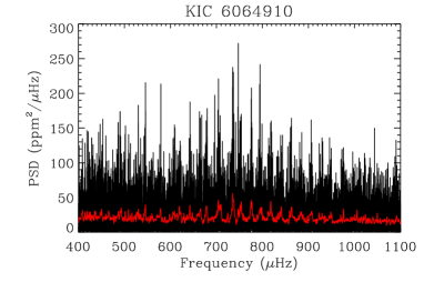
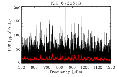
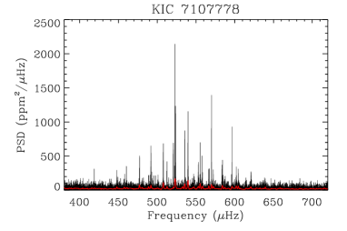
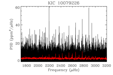
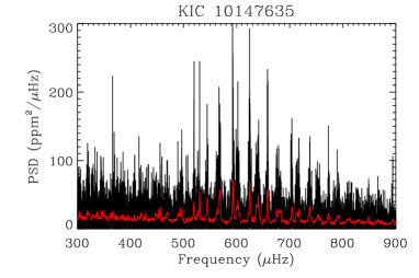
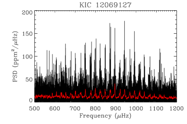
Figure 1 displays the raw power spectra of the six targets in black and smoothed one using a Gaussian-weighted window function in red in the oscillation range. Note that the smoothed power spectra are only used to enhance the appearance, and we did not use them in the following data analysis.
3.2 Global asteroseismic parameters
Mean large separation indicates the mean value of separations between two neighboring modes. It measures the pace of the increase of non-radial modes. Therefore, it can be derived utilizing the autocorrelation function (ACF) (e.g. Roxburgh & Vorontsov 2006; Tian et al. 2014), since ACF of a series yields information about the period. ACF of is defined as
| (1) |
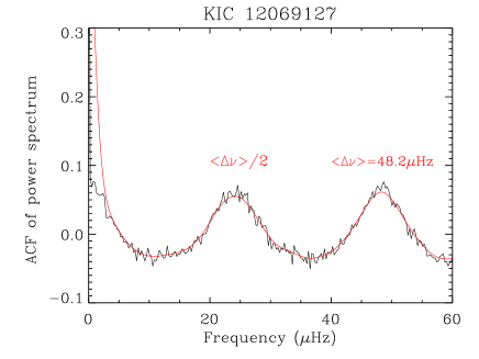
where “E” is the expected value operator, and and are the mean and variance respectively. The larger the ACF is, the stronger relation it shows at this specific phase , which is more likely to be . We applied the ACF method to the power spectra and found several peaks.
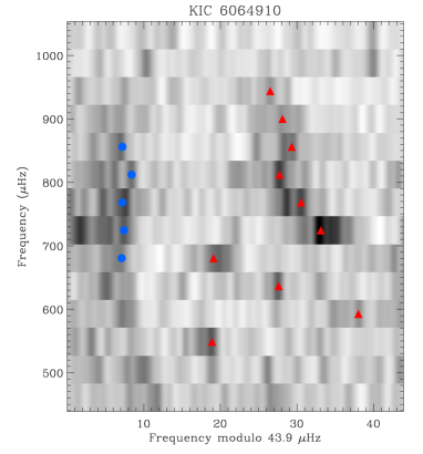
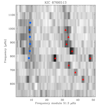
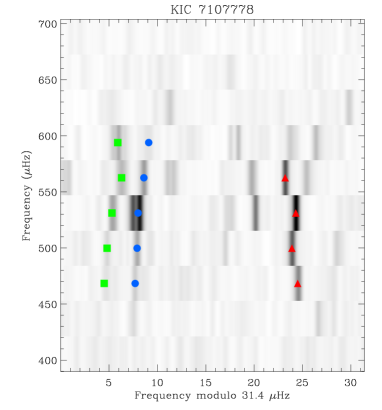
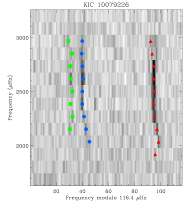
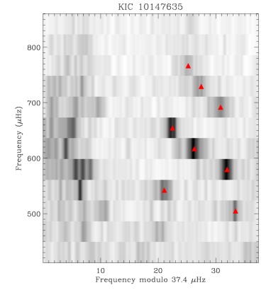
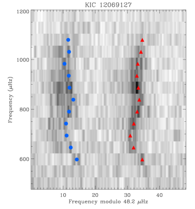
Figure 2 shows the ACF of KIC 12069127 as an example. Note that the first peak appears at , and it is caused by overlap between and modes. This requires us to be careful when examining our results. We validated with two methods. First, we took the Fourier transformation of the power spectrum in the oscillation range. A peak is expected to be found around . Second, we used to plot the échelle diagram. It extracts sections of the power spectrum in the space of and stacks them from bottom to top. Amplitudes of power density are displayed on a color scale. The right should make échelle diagram display clear pulsation patterns. For instance, we expect to see three ridges on it for main-sequence stars, corresponding to modes. The patterns become more complicated when the stars evolve (discussed later), but are still recognizable. Figure 3 shows the échelle diagram of six stars.
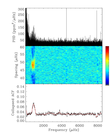
Frequency of maximum power measures the location of power excess. It can be obtained by heavily smoothing the power spectrum and the central frequency is denoted by (Chaplin et al. 2008; Stello et al. 2009a). Here, we checked this result by collapsed ACF, according to Huber et al. (2009). First, we split the power spectrum into the same logarithmic bins, and smooth them with a median filter as the background of the power spectrum. Second, we subtract the background derived above from the raw power spectrum, and divide the residual power spectrum into subsets roughly equal to 4 with an overlap. We calculated ACF for each subset. Third, we collapse the ACF of each subset over all frequency spacing. We fit the collapsed ACF with a Gaussian profile and its frequency of maximum value is believed to be .
Figure 4 shows the power spectrum of KIC 12069127 in the top panel, together with ACF of each subset for each spacing in the middle panel, and collapsed ACF in the bottom panel.
After we checked our results with different approaches for quality assurance, we compared our results, both and , to previous literature. Chaplin et al. (2014) only used the first ten months of Kepler data, and for the case of our six targets, only one month SC data was used.
Table 2 shows results from the two works. We note that shows good accordance, while has slight deviations. This may be due to two reasons. First, we used different data, as illustrated above. Second, the definition of is slightly ambiguous, so that it carries an intrinsic uncertainty. Furthermore, the choices of different smoothing function may enhance the uncertainty. Because the differences are not that large and does not show strong constraints on the following stellar models, we then omitted them.
3.3 Oscillation Frequencies
In order to excavate deeper seismic information, we extracted oscillaion frequencies of the six targets. We started by reviewing characteristics of solar-like oscillation. The signature of p modes can be well described using asymptotic theory controlled by radial order and angular degree . The approximate expression can be written as (Tassoul 1980):
| (2) |
where coefficient and depend on stellar conditions. This expression indicates p mode frequencies are equally spaced in frequency (i.e. ). The large separation is related to the sound radius through:
| (3) |
and and are the sound speed and the stellar radius, respectively. is related to the acoustic diameter. Higher order of g modes can also be described by an asymptotic relation (Tassoul 1980):
| (4) |
where
| (5) |
where is the buoyancy frequency which controls the behavior of g modes and is given by
| (6) |
This indicates g mode frequencies are placed equally spaced in period (i.e. ).
Several methods to extract oscillation frequencies in a global way have been put forward, for example, Bayesian Markov Chain Monte Carlo (Handberg & Campante 2011; Benomar 2008), Maximum Likelihood Estimation (Appourchaux et al. 1998); however, when the power spectrum reveal p and g mixed modes with low S/N, global analysis is not advantageous, because there exist several frequencies that are hard to determine, and it is easy for an automatic program to wrongly determine these frequencies. Therefore, here we derived them separately based on asymptotic theory and visual inspection. The identified modes are fitted with Lorentzian profiles using the least-squares minimization. The Lorentzian model is:
| (7) |
where the three free parameters are amplitude , frequency centroid , and linewidth . We regard as the oscillation frequency. The objective function is written as,
| (8) |
where is the power spectrum density. The objective function can be minimized by taking partial derivatives and setting to zero, i.e.
| (9) | |||
Values for frequency centroid are derived by solving the above set of non-linear equations.
We present individual mode frequencies in Table 3. For KIC 7107778 and KIC 10079226, we obtained their modes with . For KIC 6064910, KIC 6766513 and KIC 12069127, we obtained their modes with . modes of those stars are difficult to identify due to low S/N. For KIC 10147635, only modes with were extracted, because the modes were significantly mixed. In figure 3, We mark the identified modes with circles, triangles, and squares for and , respectively.
4 Grid modeling
Some stellar fundamental parameters, e.g. , , can be directly deduced by seismic parameters (discussed below). However, to further investigate and analyze the six targets comprehensively, we constructed stellar grid models. The main theme of grid modeling is to construct models in a large range and select models which meet the constraints, including seismic constraints (e.g. and ) and non-seismic constraints (e.g. stellar atmospheric parameters). The properties of these qualified models are regarded as properties of the stars.
4.1 Modeling parameters and input physics
We computed stellar models with the Yale Rotating Stellar Evolution Code (Demarque et al. 2008; Pinsonneault et al. 1990; Pinsonneault et al. 1992). The input parameter, mass was estimated with scaling relations. Mean large separation is related to mean density of the star, i.e. , and the frequency of maximum power is related to both surface gravity and effective temperature of the star, i.e. (e.g. Christensen-Dalsgaard 1993 and Kjeldsen & Bedding 1995). Hence, and can be expressed in terms of the solar values:
| (10) |
| (11) |
where , (Chaplin & Miglio 2013) and K. Combining the two equations above, we obtained
| (12) |
This requires the grid should at least cover , considering uncertainties associated with each parameter. Spectroscopic observation requires of the grid range from . We ignored convection overshooting and treated convection with standard mixing-length theory (Böhm-Vitense 1958), with three mixing parameters 1.75, 1.84 and 1.95. In particular, 1.84 originates from the solar calibrated model of YREC (see Wu et al. 2016). The free input parameters mass , initial metallicity [Fe/H] and mixing length parameter , are summarized in Table 4.
The input physics is set as follows. We adopted NACRE Nuclear reaction rates in Bahcall et al. (1995), equation of state tables in Rogers & Nayfonov (2002), OPAL high-temperature opacities in Iglesias & Rogers (1996), and low-temperature opacities in Ferguson et al. (2005). Atomic diffusion was considered only under initial masses , with the formulation of Thoul et al. (1994). The element abundance ratio was estimated by
| (13) |
where (Grevesse & Sauval 1998). We treated the initial helium abundance of these models as
| (14) |
where , which also comes from a solar calibrated model (Wu et al. 2016). All models were calculated from Hayashi lines to red giant branch.
4.2 Constraining models
We selected qualified models of the six targets, which match the requirements imposed by observational constraints: , , and (Table 1 and 2). The qualifications were estimated with a Bayesian approach (Basu et al. 2010; Kallinger et al. 2010).
We assigned an overall probability for each model , with respect to posterior probability and observations . According to Bayes’ theorem,
| (15) |
The prior probability is set to a uniform value:
| (16) |
with being the number of models. The likelihood is expressed as,
| (17) |
where
| (18) |
| (19) |
| (20) |
| (21) |
with subscript “obs” and “model” being observation and model values respectively. The four parameters that compose the likelihood were measured independently, so the multiplication makes sense. Note that the model values of and are derived with a scaling relation. The normalization factor can be added from each model probability
| (22) |
By canceling out the constant prior probabilities, the Bayes’ theorem simplifies to
| (23) |
The above equation is used to derive posterior probability for each model. By constructing the marginal probability distribution of each parameter, we estimated their values and assigned a 1 deviation from median values as the uncertainties.
The oscillation patterns revealed from the corresponding ’echelle diagram, i.e. figure 3, accompanied by the identified oscillation frequencies , indicate the evolutionary stage of these stars. The plot for KIC 10079226 have three nearly perpendicular ridges, suggesting it is a main-sequence star with p mode oscillations. KIC 12069127 is also “main-sequence like”. Evolved stars turn out to show p-g mixed modes for . An identifying signature is that modes deviate from the ridge, and overlap to form a slope, for example, KIC 6064910, KIC 6766513 and KIC 10147635. Additionally, KIC 7107778 displays a more sophisticate pattern, partly because it is more evolved than the others.
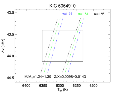
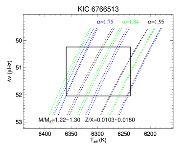
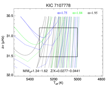
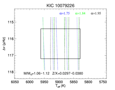
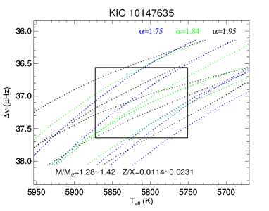
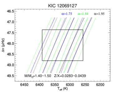
Figure 5 shows the evolution tracks with models falling into error boxes (black solid squares) on the - diagram. The error boxes are multidimensional (but are displayed as a plane here), representing constraints from , , and [Fe/H]. Models with mixing length parameter 1.75, 1.84, and 1.95 are displayed in blue, green and black dotted lines. At the main-sequence stage, the star will go through a rather stable process when the temperature changes little with decreasing. The sub-giant star experiences a rapid temperature decline, and with decreasing. A red giant star is stably burning the hydrogen shell with an equable temperature, and continues to decrease. Therefore, we note that KIC 10079226 is still in the main-sequence stage, and the rest of them are sub-giant stars. According to our previous analysis on oscillation behavior, KIC 12069127 is “main-sequence like”, but here it turns out to be a sub-giant star. This is because it is still at the early stage of a sub-giant, when p modes are not quite affected by g modes, so that the “avoided crossing” effects are weaker. The other stars are in good accordance with their oscillation behavior on the échelle diagram.
Table 5 presents model parameters estimated by the Bayesian approach, together with those estimated by Chaplin et al. (2014). Results from the two studies indeed indicate some difference. The difference in mass even reaches , e.g. KIC 6064910, KIC 6766513, and KIC 10147635. This may caused by systematic errors associated with the grid and different inputs for , [Fe/H]. Their estimations are based on coupling BeSPP to the GARSTEC grid. Their input are from SDSS recalibration and infra-red flux method calibration, both photometrically based, while ours are based on LAMOST spectroscopic observations, so that the above three stars have a significant difference. In addition, they adopted a uniform [Fe/H] of , while we used values from LSP3.
Also, we compared the derived from LSP3 and this work. Figure 6 displays the comparison, where the blue solid line represents the equality. The results from the two work show a large difference, and the results from our work have small uncertainties, while those from LSP3 do not.
5 Conclusions
We performed data processing and asteroseismic analysis on six solar-like stars both observed by both the Kepler mission and LAMOST, and combined stellar grid models to determine stellar fundamental parameters.
We derived asteroseismic parameters and of the six targets using ACF and collapsed ACF. Individual mode frequencies were extracted with Lorentzian profiles using a least-squares fit. For KIC 7107778 and KIC 10079226, we obtained the mode frequencies with . For KIC 6064910, KIC 6766513, and KIC 12069127, we obtained the mode frequencies with . Note that with are more reliable than with for these three stars, for the mix of and modes make them relatively ambiguous. Modes of KIC 10147635 were only obtained with due to relatively low S/N.
According to numerical solutions of the stellar models, we looked into the evolutionary stages of the six solar-like targets and categorized them into one main-sequence star (KIC 10079226) and five sub-giant stars (the others), four of which show strong characteristics of p and g mixed modes. Grid modeling indicates that the five sub-giant stars are in the range of and , and the main-sequence star has corresponding values of and . Their ages are in the range of . Ages of most stars can reach an accuracy under 1 , reflecting the capabilities of asteroseismology, but KIC 7107778 and KIC 10079226 have larger uncertainties in age.
In this work, we do not use individual oscillation frequencies to constrain stellar models. and have shown their potential on constraining models, but individual oscillation frequencies can constrain them in a more powerful way. This will be presented in our follow-up research.
Acknowledgements.
The author would like to thank the whole Kepler and LAMOST team, who make these results possible. We also greatly acknowledge the support provided by National College Students Innovation Training Program. This work is supported by grants 11273007 and 10933002 from the National Natural Science Foundation of China, the Joint Research Fund in Astronomy (U1631236) under cooperative agreement between the National Natural Science Foundation of China (NSFC) and Chinese Academy of Sciences (CAS), and the Fundamental Research Funds for the Central Universities.References
- Aizenman et al. (1977) Aizenman, M., Smeyers, P., & Weigert, A. 1977, A&A, 58, 41
- Appourchaux et al. (1998) Appourchaux, T., Gizon, L., & Rabello-Soares, M.-C. 1998, A&AS, 132, 107
- Appourchaux et al. (2008) Appourchaux, T., Michel, E., Auvergne, M., et al. 2008, A&A, 488, 705
- Appourchaux et al. (2012) Appourchaux, T., Chaplin, W. J., García, R. A., et al. 2012, A&A, 543, A54
- Appourchaux et al. (2014) Appourchaux, T., Antia, H. M., Benomar, O., et al. 2014, A&A, 566, A20
- Bahcall et al. (1995) Bahcall, J. N., Pinsonneault, M. H., & Wasserburg, G. J. 1995, Reviews of Modern Physics, 67, 781
- Basu et al. (2010) Basu, S., Chaplin, W. J., & Elsworth, Y. 2010, ApJ, 710, 1596
- Benomar (2008) Benomar, O. 2008, Communications in Asteroseismology, 157, 98
- Benomar et al. (2012) Benomar, O., Bedding, T. R., Stello, D., et al. 2012, ApJ, 745, L33
- Benomar et al. (2014) Benomar, O., Belkacem, K., Bedding, T. R., et al. 2014, ApJ, 781, L29
- Böhm-Vitense (1958) Böhm-Vitense, E. 1958, ZAp, 46, 108
- Borucki et al. (2007) Borucki, W. J., Koch, D. G., Lissauer, J. J., et al. 2007, in Bulletin of the American Astronomical Society, Vol. 39, American Astronomical Society Meeting Abstracts #210, 235
- Campante et al. (2015) Campante, T. L., Barclay, T., Swift, J. J., et al. 2015, in European Physical Journal Web of Conferences, Vol. 101, European Physical Journal Web of Conferences, 02004
- Casanellas (2015) Casanellas, J. 2015, in European Physical Journal Web of Conferences, Vol. 101, European Physical Journal Web of Conferences, 01015
- Chaplin et al. (2008) Chaplin, W. J., Houdek, G., Appourchaux, T., et al. 2008, A&A, 485, 813
- Chaplin & Miglio (2013) Chaplin, W. J., & Miglio, A. 2013, ARA&A, 51, 353
- Chaplin et al. (2014) Chaplin, W. J., Basu, S., Huber, D., et al. 2014, ApJS, 210, 1
- Christensen-Dalsgaard (1982) Christensen-Dalsgaard, J. 1982, Advances in Space Research, 2, 11
- Christensen-Dalsgaard (1993) Christensen-Dalsgaard, J. 1993, in Astronomical Society of the Pacific Conference Series, Vol. 42, GONG 1992. Seismic Investigation of the Sun and Stars, ed. T. M. Brown, 347
- Christensen-Dalsgaard & Frandsen (1983) Christensen-Dalsgaard, J., & Frandsen, S. 1983, Sol. Phys., 82, 469
- Davies et al. (2016) Davies, G. R., Silva Aguirre, V., Bedding, T. R., et al. 2016, MNRAS, 456, 2183
- Deheuvels et al. (2012) Deheuvels, S., García, R. A., Chaplin, W. J., et al. 2012, ApJ, 756, 19
- Demarque et al. (2008) Demarque, P., Guenther, D. B., Li, L. H., Mazumdar, A., & Straka, C. W. 2008, Ap&SS, 316, 31
- Doǧan et al. (2013) Doǧan, G., Metcalfe, T. S., Deheuvels, S., et al. 2013, ApJ, 763, 49
- Ferguson et al. (2005) Ferguson, J. W., Alexander, D. R., Allard, F., et al. 2005, ApJ, 623, 585
- García et al. (2011) García, R. A., Hekker, S., Stello, D., et al. 2011, MNRAS, 414, L6
- Gilliland et al. (2010) Gilliland, R. L., McCullough, P. R., Nelan, E. P., et al. 2010, arXiv:1011.0435
- Grevesse & Sauval (1998) Grevesse, N., & Sauval, A. J. 1998, Space Sci. Rev., 85, 161
- Gruberbauer et al. (2013) Gruberbauer, M., Guenther, D. B., MacLeod, K., & Kallinger, T. 2013, MNRAS, 435, 242
- Handberg & Campante (2011) Handberg, R., & Campante, T. L. 2011, A&A, 527, A56
- Houdek et al. (1999) Houdek, G., Balmforth, N. J., Christensen-Dalsgaard, J., & Gough, D. O. 1999, A&A, 351, 582
- Huang et al. (2015) Huang, Y., Liu, X.-W., Yuan, H.-B., et al. 2015, MNRAS, 454, 2863
- Huber et al. (2009) Huber, D., Stello, D., Bedding, T. R., et al. 2009, Communications in Asteroseismology, 160, 74
- Iglesias & Rogers (1996) Iglesias, C. A., & Rogers, F. J. 1996, ApJ, 464, 943
- Kallinger et al. (2010) Kallinger, T., Mosser, B., Hekker, S., et al. 2010, A&A, 522, A1
- Kjeldsen & Bedding (1995) Kjeldsen, H., & Bedding, T. R. 1995, 293, astro-ph/9403015
- Lagarde et al. (2015) Lagarde, N., Miglio, A., Eggenberger, P., et al. 2015, A&A, 580, A141
- Liu et al. (2014) Liu, Z., Yang, W., Bi, S., et al. 2014, ApJ, 780, 152
- Lomb (1976) Lomb, N. R. 1976, Ap&SS, 39, 447
- Metcalfe et al. (2010) Metcalfe, T. S., Monteiro, M. J. P. F. G., Thompson, M. J., et al. 2010, ApJ, 723, 1583
- Montalbán & Noels (2013) Montalbán, J., & Noels, A. 2013, in European Physical Journal Web of Conferences, Vol. 43, European Physical Journal Web of Conferences, 03002
- Mosser (2015) Mosser, B. 2015, in European Physical Journal Web of Conferences, Vol. 101, European Physical Journal Web of Conferences, 01001
- Mosser et al. (2014) Mosser, B., Benomar, O., Belkacem, K., et al. 2014, A&A, 572, L5
- Ozel et al. (2010) Ozel, N., Dupret, M.-A., & Baglin, A. 2010, Ap&SS, 328, 67
- Pinsonneault et al. (1990) Pinsonneault, M. H., Deliyannis, C. P., & Demarque, P. 1990, in BAAS, Vol. 22, Bulletin of the American Astronomical Society, 746
- Pinsonneault et al. (1992) Pinsonneault, M. H., Deliyannis, C. P., & Demarque, P. 1992, ApJS, 78, 179
- Ren et al. (2016) Ren, J.-J., Liu, X.-W., Xiang, M.-S., et al. 2016, Research in Astronomy and Astrophysics, 16, 45
- Rogers & Nayfonov (2002) Rogers, F. J., & Nayfonov, A. 2002, ApJ, 576, 1064
- Roxburgh & Vorontsov (2006) Roxburgh, I. W., & Vorontsov, S. V. 2006, MNRAS, 369, 1491
- Scargle (1982) Scargle, J. D. 1982, ApJ, 263, 835
- Sharma et al. (2016) Sharma, S., Stello, D., Bland-Hawthorn, J., Huber, D., & Bedding, T. R. 2016, ApJ, 822, 15
- Silva Aguirre et al. (2014) Silva Aguirre, V., Casagrande, L., & Miglio, A. 2014, in IAU Symposium, Vol. 298, Setting the scene for Gaia and LAMOST, ed. S. Feltzing, G. Zhao, N. A. Walton, & P. Whitelock, 375
- Silva Aguirre et al. (2013) Silva Aguirre, V., Basu, S., Brandão, I. M., et al. 2013, ApJ, 769, 141
- Soriano et al. (2007) Soriano, M., Vauclair, S., Vauclair, G., & Laymand, M. 2007, A&A, 471, 885
- Stello et al. (2009a) Stello, D., Chaplin, W. J., Basu, S., Elsworth, Y., & Bedding, T. R. 2009a, MNRAS, 400, L80
- Stello et al. (2009b) Stello, D., Chaplin, W. J., Bruntt, H., et al. 2009b, ApJ, 700, 1589
- Tassoul (1980) Tassoul, M. 1980, ApJS, 43, 469
- Thoul et al. (1994) Thoul, A. A., Bahcall, J. N., & Loeb, A. 1994, ApJ, 421, 828
- Tian et al. (2014) Tian, Z. J., Bi, S. L., Yang, W. M., et al. 2014, MNRAS, 445, 2999
- Verner et al. (2011) Verner, G. A., Elsworth, Y., Chaplin, W. J., et al. 2011, MNRAS, 415, 3539
- Wu et al. (2016) Wu, Y., Xiang, M., Zhang, X., et al. 2016, arXiv:1609.05707
- Xiang et al. (2015a) Xiang, M. S., Liu, X. W., Yuan, H. B., et al. 2015a, MNRAS, 448, 90
- Xiang et al. (2015b) Xiang, M. S., Liu, X. W., Yuan, H. B., et al. 2015b, VizieR Online Data Catalog, 744
- Xiang et al. (2016) Xiang, M.-S., Liu, X.-W., Shi, J.-R., et al. 2016, arXiv:1610.00083
- Yang et al. (2015) Yang, W., Tian, Z., Bi, S., et al. 2015, MNRAS, 453, 2094
| NO. | KIC | Kepler data | ||||
|---|---|---|---|---|---|---|
| (Q) | ||||||
| 1 | 6064910 | 7.111.3 | 628659 | 3.740.09 | -0.330.08 | |
| 2 | 6766513 | 7.111.3 | 629461 | 3.880.08 | -0.180.07 | |
| 3 | 7107778 | 7.111.3 | 5118191 | 3.530.08 | 0.070.13 | |
| 4 | 10079226 | 7.110.3 | 588961 | 4.440.11 | 0.110.06 | |
| 5 | 10147635 | 7.111.3 | 581459 | 4.670.26 | -0.080.18 | |
| 6 | 12069127 | 7.111.3 | 630564 | 3.950.10 | 0.160.08 |
0.86“Q” represents three-month-long observation quarter. Atmospheric parameters were derived by LSP3 (Xiang et al. 2015b).
| KIC | |||||
|---|---|---|---|---|---|
| 1 | 6064910 | 43.900.40 | 43.900.80 | 73337 | 72143 |
| 2 | 6766513 | 51.300.99 | 51.301.10 | 83290 | 88384 |
| 3 | 7107778 | 31.400.34 | 31.400.34 | 54019 | 54019 |
| 4 | 10079226 | 116.400.86 | 116.41.9 | 2588135 | 268993 |
| 5 | 10147635 | 37.400.54 | 37.400.50 | 58228 | 63420 |
| 6 | 12069127 | 48.200.80 | 48.200.90 | 81750 | 82941 |
0.86(a): results in this work; (b): results from Chaplin et al. (2014).
| KIC 6064910 | KIC 6766513 | KIC 7107778 | KIC 10079226 | KIC 10147635 | KIC 12069127 | |
|---|---|---|---|---|---|---|
| … | ||||||
| … | … | |||||
| … | ||||||
| … | ||||||
| … | ||||||
| … | ||||||
| … | ||||||
| … | … | |||||
| … | … | … | … | |||
| … | ||||||
| Variable | Value |
|---|---|
| Mass | , |
| , | |
| 1.75, 1.84, 1.95 |
| KIC | ||||||||||||||
|---|---|---|---|---|---|---|---|---|---|---|---|---|---|---|
| () | () | () | () | () | () | (Gyr) | (Gyr) | (Gyr) | (dex) | (dex) | (dex) | () | (K) | |
| 6064910 | ||||||||||||||
| 6766513 | ||||||||||||||
| 7107778 | ||||||||||||||
| 10079226 | ||||||||||||||
| 10147635 | ||||||||||||||
| 12069127 |
