A New Continuum Formulation for Materials–Part II. Some Applications in Fluid Mechanics

Abstract

In part I of this paper, I proposed a new set of equations, which I refer to as the $\overline{M}\left(D,\eta\right)$-formulation and which differs from the Navier-Stokes-Fourier description of fluid motion.  Here, I use these equations to model several classic examples in fluid mechanics, with the intention of providing a general sense of comparison between the two approaches.  A few broad facts emerge: (1) it is as simple–or in most cases, much simpler–to find solutions with the $\overline{M}\left(D,\eta\right)$-formulation, (2) for some examples, there is not much of a difference in predictions–in fact, for sound propagation and for examples in which there is only a rotational part of the velocity, my transport coefficients $D$ and $\eta$ are chosen to match Navier-Stokes-Fourier solutions in the appropriate regimes, (3) there are, however, examples in which pronounced differences in predictions appear, such as light scattering, and (4) there arise, moreover, important conceptual differences, as seen in examples like sound at a non-infinite impedance boundary, thermophoresis, and gravity’s effect on the atmosphere.

1 Introduction

In choosing the examples that appear in this paper, I desired the simplest mathematics and closed-form solutions wherever possible.  To this end, (1) variation is limited to one spatial dimension in all sections but §7 on hydrodynamical fluctuations and §10 on Poiseuille flow, (2) equations are linearized about a constant state in all sections but §12 on shock waves, and (3) parameters are chosen to yield phenomena strictly in the hydrodynamic (small $K\!n$) regime in all sections but §12.  Furthermore, so as not to distract from the main results, for examples that require any mathematical complexity, such as the stochastical subjects of §7 and §8, I provide guiding references and outline steps, but for the most part I merely present and discuss the solutions.  I will treat these problems–and others that are examined only superficially here, like stability and sound propagation–with rigor in future papers.

In addition, these particular examples were chosen to exhibit a wide variety of phenomena–including ones that connect the two theories and so provide anchoring points to tie $\overline{M}\left(D,\eta\right)$-formulation parameters to those of Navier-Stokes-Fourier (NSF), and ones that reveal major differences both measurably in experiment and conceptually.

The following is a brief description of the examples this paper contains.

• A one-dimensional linear stability analysis is carried out in §3 to show that my formulation is unconditionally stable provided that the diffusion parameter, $D$, is positive.

• In §4, a mass equilibration problem with no mechanical forces is studied in order to show that my formulation reduces to one of pure diffusion governed by Fick’s law.

• Low amplitude sound propagation, which is the subject of §5, is demonstrated to be a way of relating my longitudinal diffusion parameter, $D$, to the transport parameters of the NSF formulation by matching attenuations in the hydrodynamic regime.  I employ this relationship to estimate values of $D$ for several different gases and liquids, and these are presented in appendix C.

• In §6, acoustic impedance at a sound barrier is discussed.  In particular, I point out that the $\overline{M}\left(D,\eta\right)$-formulation allows an impermeable boundary with a non-zero normal velocity at that boundary, as that which occurs in the case of non-infinite impedance.

• As a step towards bridging the gap between microscopic and macroscopic scales in my theory, the subject of hydrodynamical fluctuations is addressed in §7, where it is shown that the thermodynamic interpretation of a continuum mechanical point (i.e. a point occupied by matter and moving with velocity $\underline{v}$) stemming from the $\overline{M}\left(D,\eta\right)$-formulation is fundamentally different from that of Navier-Stokes-Fourier.  That is, in the NSF theory, a continuum mechanical point is viewed as a thermodynamic subsystem in contact with its surrounding material which acts as a heat reservoir; whereas in my theory, the surrounding material acts not only as a heat–but also a particle–reservoir.

• The light scattering spectra from the $\overline{M}\left(D,\eta\right)$-formulation and the NSF equations are provided in §8.  Comparing these, one finds the shifted Brillouin peaks, which correspond to the sound (phonon) part of the spectrum, are virtually indistinguishable between the two theories, as one would expect, but the central Rayleigh peak predictions are significantly different.  For example, in a classical monatomic ideal gas in the hydrodynamic regime, the $\overline{M}\left(D,\eta\right)$-formulation predicts a Rayleigh peak that is about $29\%$ taller and narrower than the NSF equations (but with the same area so that the well-verified Landau-Placzek ratio remains intact).  Previous experimenters, e.g. Clark [7] and Fookson et al. [13], did not study gases fully in the hydrodynamic regime, $K\!n\lesssim O\left(10^{-2}\right)$, choosing instead to focus on more rarefied gases with Knudsen numbers in the range, $O\left(10^{-1}\right)\lesssim K\!n\lesssim O\left(1\right)$, which extends into the slip flow and transition regimes.  Therefore, in order to verify the $\overline{M}\left(D,\eta\right)$-formulation, it is important to conduct a high-resolution light scattering experiment for a gas in the hydrodynamic regime.

• In §9, I study the effect of gravity on the Earth’s lower atmosphere, and show that enforcing no mass flux and no total energy flux conditions in the $\overline{M}\left(D,\eta\right)$-formulation, leads to the isentropic condition that is typically assumed a priori.  In contrast, enforcing the same conditions in the NSF formulation, leads to an isothermal condition, which is obviously not physical.

• Poiseuille flow is the subject of §10.  There, I show that, when compared to the NSF mass flow rate, which is due solely to convection, the $\overline{M}\left(D,\eta\right)$-formulation predicts an additional contribution due to diffusion.  In the hydrodynamic regime, however, this contribution is very small, and so these predictions do not differ by much.  Since viscometers may be based on Poiseuille flow, this–and other examples of this sort–provide justification that the shear viscosity appearing in the $\overline{M}\left(D,\eta\right)$-formulation may be taken to be the same as the Navier-Stokes shear viscosity.

• Thermophoresis, or the down-temperature-gradient motion of a macroscopic particle in a resting fluid, is discussed in §11.  For an idealized problem, it is shown that, through the steady-state balancing of the convective and diffusive terms of the mass flux, the $\overline{M}\left(D,\eta\right)$-formulation provides a mechanism for thermophoresis that is not present in the NSF formulation.  In the latter type, a thermal slip boundary condition at the particle’s surface is needed in order to model thermophoretic motion, whereas the former type may be used to describe this motion with a no-slip boundary condition, i.e. one in which the tangential velocity of the particle at its surface equals that of the fluid.  The concept of thermal slip is based on kinetic gas theory arguments in the slip flow regime, appropriate for $K\!n\gtrsim O\left(10^{-2}\right)$, yet thermophoresis is observed in gases for much smaller Knudsen numbers in the hydrodynamic regime and also in liquids.  Therefore, there are obvious advantages to being able to model this problem without the thermal slip condition.

• A non-linear steady-state shock wave problem is considered in §12.  It is well-known that for this problem, the NSF formulation–and all other accepted theories, for that matter–produces normalized density, velocity, and temperature shock wave profiles that are appreciably displaced from one another with the temperature profile in the leading edge of the shock, velocity behind it, and density trailing in the back.  The $\overline{M}\left(D,\eta\right)$-formulation, however, predicts virtually no displacement between these three profiles in the leading edge of the shock and much less pronounced displacements in the middle and trailing end of the shock.

2 Equations of Motion from Part I

All formulas referenced from part I of this paper are labeled with ”I.” preceding their number.  As derived in part I, the $\overline{M}\left(D,\eta\right)$-formulation consists of the balance laws (I.43):

$$\frac{\partial\overline{m}}{\partial t} =-\nabla\cdot\left(\overline{m}\underline{v}\right)$$

$$\frac{\partial m}{\partial t} =-\nabla\cdot\left(\underline{q}_{M}+m\underline{v}\right)$$ (1)

$$\frac{\partial\left(\overline{m}\underline{v}\right)}{\partial t} =-\nabla\cdot\left(\underline{\underline{P}}+\overline{m}\underline{v}\,\underline{v}\right)+\overline{m}\underline{f}_{\overline{M}}$$

$$\frac{\partial u}{\partial t} =-\nabla\cdot\left(\underline{q}_{U}+u\underline{v}\right)-\underline{\underline{P}}\colon\nabla\underline{v}$$

with constitutive equations (I.74):

$$\underline{q}_{M} =-D\nabla m$$

$$\underline{\underline{P}} =P\underline{\underline{1}}+\underline{\underline{P}}_{\text{visc}}\text{ with }\underline{\underline{P}}_{\text{visc}}=\left[\begin{array}[c]{c}-\left(\overline{m}D-\frac{4\eta}{3}\right)\left(\nabla\cdot\underline{v}\right)\underline{\underline{1}}-\\ 2\eta\left(\nabla\underline{v}\right)^{sy,dev}\end{array}\right]$$ (4)

$$\underline{q}_{U} =-D\nabla u.$$

The Navier-Stokes-Fourier formulation is given by the balance laws (I.45):

$$\frac{\partial m}{\partial t} =-\nabla\cdot\left(m\underline{v}\right)$$

$$\frac{\partial\left(m\underline{v}\right)}{\partial t} =-\nabla\cdot\left(\underline{\underline{P}}+m\underline{v}\,\underline{v}\right)+m\underline{f}_{M}$$ (5)

$$\frac{\partial u}{\partial t} =-\nabla\cdot\left(\underline{q}_{U}+u\underline{v}\right)-\underline{\underline{P}}\colon\nabla\underline{v}$$

with constitutive equations (I.46):

$$\underline{\underline{P}} =P\underline{\underline{I}}+\underline{\underline{P}}_{\text{visc}}\text{ with }\underline{\underline{P}}_{\text{visc}}=-\zeta_{NS}\left(\nabla\cdot\underline{v}\right)\underline{\underline{I}}-2\eta\left(\nabla\underline{v}\right)^{sy,dev}$$ (6)

$$\underline{q}_{U} =-k_{F}\nabla T.$$

Other quantities employed in this paper that hold for both formulations when the proper constitutive equations are used are the total energy balance law (I.8)/(I.20),

$$\frac{\partial e}{\partial t}=-\nabla\cdot\left(\underline{q}_{U}+\underline{\underline{P}}\cdot\underline{v}+e\underline{v}\right),$$ (7)

the total energy flux,

$$\underline{j}_{E}=\underline{q}_{U}+\underline{\underline{P}}\cdot\underline{v}+e\underline{v},$$ (8)

and the total mass flux,

$$\underline{j}_{M}=\underline{q}_{M}+m\underline{v}.$$ (9)

To solve the steady-state examples of §9-11, one may derive the following convenient forms for the two formulations considered here.  First, taking the balance laws (1 a-c) and (7) with constitutive equations (4), setting the time-derivatives equal to zero for a steady state, using thermodynamic relationships (293) and (294) to express the equations in terms of the variables $\overline{m}$, $P$, $\underline{v}$, and $T$, and linearizing about a constant state,

$$\left(\overline{m},P,\underline{v},T\right)=\left(m_{\ast},P_{\ast},\underline{0},T_{\ast}\right),$$ (10)

one obtains

$$0 =-m_{\ast}\nabla\cdot\underline{v}$$

$$0 =D_{\ast}\left[-\left(m\alpha_{P}\right)_{\ast}\nabla^{2}T+\left(\frac{\gamma}{c^{2}}\right)_{\ast}\nabla^{2}P\right]-m_{\ast}\nabla\cdot\underline{v}$$ (11)

$$0 =-\nabla P+\left(\overline{m}D-\frac{4\eta}{3}\right)_{\ast}\nabla\left(\nabla\cdot\underline{v}\right)+2\eta_{\ast}\nabla\cdot\left[\left(\nabla\underline{v}\right)^{sy,dev}\right]$$

$$0 =D_{\ast}\left\{\begin{array}[c]{c}\left[m\left(c_{P}-h_{M}\alpha_{P}\right)\right]_{\ast}\nabla^{2}T+\\ \left(\frac{h_{M}\gamma}{c^{2}}-T\alpha_{P}\right)_{\ast}\nabla^{2}P\end{array}\right\}-\left(mh_{M}\right)_{\ast}\nabla\cdot\underline{v}.$$ (14)

If we then substitute (11 a) into (11 c-d) and employ the tensor identity (275), the above equations imply that for the $\overline{M}\left(D,\eta\right)$-formulation,

$$0 =\nabla\cdot\underline{v}$$

$$0 =\nabla^{2}P$$ (15)

$$0 =-\nabla P+\eta_{\ast}\nabla^{2}\underline{v}+m_{\ast}f_{\overline{M}}$$

$$0 =\nabla^{2}T.$$

In addition, by substituting constitutive relations (4) into equations (8) and (9), employing thermodynamic relations (293), (294), and (287), and linearizing about constant state (10), one finds the following total energy and mass fluxes for the $\overline{M}\left(D,\eta\right)$-formulation:

$$\underline{j}_{E}=-D_{\ast}\left\{\begin{array}[c]{c}\left[m\left(c_{P}-h_{M}\alpha_{P}\right)\right]_{\ast}\nabla T+\\ \left(\frac{h_{M}\gamma}{c^{2}}-T\alpha_{P}\right)_{\ast}\nabla P\end{array}\right\}+\left(mh_{M}\right)_{\ast}\underline{v}$$ (16)

and

$$\underline{j}_{M}=-D_{\ast}\left[-\left(m\alpha_{P}\right)_{\ast}\nabla T+\left(\frac{\gamma}{c^{2}}\right)_{\ast}\nabla P\right]+m_{\ast}\underline{v}$$ (17)

where, in addition to all of the quantities defined in part I, we have introduced the isobaric specific heat per mass $c_{P}$, isobaric to isochoric specific heat ratio $\gamma=c_{P}/c_{V}$, and adiabatic sound speed $c$.  Carrying out similar steps, yields for the NSF formulation, the steady-state equations,

$$0 =\nabla\cdot\underline{v}$$

$$0 =-\nabla P+\eta_{\ast}\nabla^{2}\underline{v}+m_{\ast}f_{M}$$ (18)

$$0 =\nabla^{2}T,$$

and the fluxes,

$$\underline{j}_{E}=-\left(k_{F}\right)_{\ast}\nabla T+\left(mh_{M}\right)_{\ast}\underline{v}$$ (19)

and

$$\underline{j}_{M}=m_{\ast}\underline{v}.$$ (20)

Notice that the set of equations (18) is identical to the set (15), except for the absence of Laplace’s equation for the pressure (15 b).  Also, the fluxes (19) and (20) have the same convective parts as the $\overline{M}\left(D,\eta\right)$-formulation fluxes (16) and (17), but differing diffusive parts (with the NSF mass flux having no diffusion at all).

3 Stability Analysis

Let us consider the Cartesian one-dimensional problem in which variation is assumed to be in the $x_{1}\equiv x$ direction only with $v_{1}\equiv v$ as the only non-zero component of the velocity and there are assumed to be no body forces.  If we use the thermodynamic relationships (291) and (292) to recast the $\overline{M}\left(D,\eta\right)$-formulation (1)/(4) in terms of the variables, $\overline{m}$, $m$, $v$, and $T$, and then linearize about the constant equilibrium state,

$$\left(\overline{m},m,v,T\right)=\left(m_{\text{eq}},m_{\text{eq}},0,T_{\text{eq}}\right),$$ (21)

via

$$\overline{m} =m_{\text{eq}}+\delta\!\overline{m}$$ (22)

$$m =m_{\text{eq}}+\delta\!m$$ (23)

$$v =\delta\!v$$ (24)

$$T =T_{\text{eq}}+\delta\!T,$$ (25)

assuming

$$\left|\delta\!\overline{m}\right|,\left|\delta\!m\right| \ll m_{\text{eq}}$$

$$\left|\delta\!T\right| \ll T_{\text{eq}}$$

$$\left|\delta\!v\right| \ll c_{\text{eq}},$$

then we arrive at the following system of linear equations:

$$\frac{\partial\delta\!\overline{m}}{\partial t} =-m_{\text{eq}}\frac{\partial\delta\!v}{\partial x}$$ (26)

$$\frac{\partial\delta\!m}{\partial t} =D_{\text{eq}}\frac{\partial^{2}\delta\!m}{\partial x^{2}}-m_{\text{eq}}\frac{\partial\delta\!v}{\partial x}$$ (27)

$$\frac{\partial\delta\!v}{\partial t} =-\frac{1}{\left(m^{2}\kappa_{T}\right)_{\text{eq}}}\frac{\partial\delta\!m}{\partial x}-\left(\frac{\alpha_{P}}{m\kappa_{T}}\right)_{\text{eq}}\frac{\partial\delta\!T}{\partial x}+D_{\text{eq}}\frac{\partial^{2}\delta\!v}{\partial x^{2}}$$ (28)

$$\frac{\partial\delta\!T}{\partial t} =D_{\text{eq}}\frac{\partial^{2}\delta\!T}{\partial x^{2}}-\left(\frac{T\alpha_{P}}{m\kappa_{T}c_{V}}\right)_{\text{eq}}\frac{\partial\delta\!v}{\partial x},$$ (29)

where the subscript ”eq” indicates that the parameter is evaluated at the constant equilibrium state (21).  Note that for this linearized problem, the mechanical mass equation (26) may be uncoupled from the rest of the system, (27)-(29).  Postulating a solution,

$$\left[\begin{array}[c]{c}\delta\!m\\ \delta\!v\\ \delta\!T\end{array}\right],$$

to (27)-(29) that is proportional to

$$\exp\left(i\kappa x+\omega t\right),$$

for $\kappa$ real and $\omega$ complex, one obtains the dispersion relation,

$$\left[\begin{array}[c]{c}\omega^{3}+3D_{\text{eq}}\kappa^{2}\omega^{2}+\left(c_{\text{eq}}^{2}+3D_{\text{eq}}^{2}\kappa^{2}\right)\kappa^{2}\omega+\\ D_{\text{eq}}\left(c_{\text{eq}}^{2}+D_{\text{eq}}^{2}\kappa^{2}\right)\kappa^{2}\end{array}\right]=0.$$ (30)

In the above, I have employed the equilibrium thermodynamic relationships (288) and (289).  Equation (30) may be solved for $\omega$ to obtain the three exact roots,

$$\omega_{1}\left(\kappa\right) =-D_{\text{eq}}\kappa^{2}$$ (31)

$$\omega_{2}\left(\kappa\right) =-D_{\text{eq}}\kappa^{2}+ic_{\text{eq}}\kappa$$ (32)

$$\omega_{3}\left(\kappa\right) =-D_{\text{eq}}\kappa^{2}-ic_{\text{eq}}\kappa.$$ (33)

Clearly, if

$$D_{\text{eq}}>0$$ (34)

is satisfied, then the real parts of $\omega_{1}\left(\kappa\right)$, $\omega_{2}\left(\kappa\right)$, and $\omega_{3}\left(\kappa\right)$, are negative for all $\kappa$, resulting in the unconditional stability of linearized system (27)-(29).

For comparison, carrying out a similar procedure with the NSF formulation (5)/(6) yields the linearization,

$$\frac{\partial\delta\!m}{\partial t} =-m_{\text{eq}}\frac{\partial\delta\!v}{\partial x}$$ (35)

$$\frac{\partial\delta\!v}{\partial t} =\left[\begin{array}[c]{c}-\frac{1}{\left(m^{2}\kappa_{T}\right)_{\text{eq}}}\frac{\partial\delta\!m}{\partial x}-\left(\frac{\alpha_{P}}{m\kappa_{T}}\right)_{\text{eq}}\frac{\partial\delta\!T}{\partial x}+\\ \left(\frac{\zeta_{NS}}{m}+\frac{4\eta}{3m}\right)_{\text{eq}}\frac{\partial^{2}\delta\!v}{\partial x^{2}}\end{array}\right]$$ (38)

$$\frac{\partial\delta\!T}{\partial t} =\left(\frac{k_{F}}{mc_{V}}\right)_{\text{eq}}\frac{\partial^{2}\delta\!T}{\partial x^{2}}-\left(\frac{T\alpha_{P}}{m\kappa_{T}c_{V}}\right)_{\text{eq}}\frac{\partial\delta\!v_{x,1}}{\partial x},$$ (39)

with the dispersion relation,

$$\left(\begin{array}[c]{c}\omega^{3}+\left[\frac{\zeta_{NS}}{m}+\left(\frac{4}{3}+E\!u\right)\frac{\eta}{m}\right]_{\text{eq}}\kappa^{2}\omega^{2}+\\ \left\{c_{\text{eq}}^{2}+\left[E\!u\left(\frac{\zeta_{NS}}{m}+\frac{4\eta}{3m}\right)\frac{\eta}{m}\right]_{\text{eq}}\kappa^{2}\right\}\kappa^{2}\omega+\\ \left(\frac{E\!u}{\gamma}\frac{\eta}{m}c^{2}\right)_{\text{eq}}\kappa^{4}\end{array}\right)=0,$$ (40)

where $\gamma$ is the ratio of specific heats and $E\!u$ is the Euken ratio defined to be

$$E\!u=\frac{k_{F}}{c_{V}\eta}.$$ (41)

Let us also define the quantities,

$$\Sigma=\frac{E\!u}{\gamma}\frac{\eta}{m}$$ (42)

and

$$\Gamma=\frac{1}{2}\left\{\frac{\zeta_{NS}}{m}+\left[\frac{4}{3}+\left(1-\frac{1}{\gamma}\right)E\!u\right]\frac{\eta}{m}\right\}.$$ (43)

Using these, equation (40) yields the following three approximate roots,

$$\omega_{1}\left(\kappa\right) \approx-\Sigma_{\text{eq}}\kappa^{2}$$ (44)

$$\omega_{2}\left(\kappa\right) \approx-\Gamma_{\text{eq}}\kappa^{2}+ic_{\text{eq}}\kappa$$ (45)

$$\omega_{3}\left(\kappa\right) \approx-\Gamma_{\text{eq}}\kappa^{2}-ic_{\text{eq}}\kappa,$$ (46)

for

$$\left(\frac{\eta}{mc}\right)_{\text{eq}}\left|\kappa\right|\ll 1,$$ (47)

which corresponds to the low Knudsen number, or hydrodynamic, regime.  For an equilibrium thermodynamically stable fluid,

$$\gamma\geq 1\text{ and }c_{V}>0$$ (48)

are satisfied, and therefore, if the standard assumption that $\eta_{\text{eq}},\left(k_{F}\right)_{\text{eq}}>0$ and $\left(\zeta_{NS}\right)_{\text{eq}}\geq 0$ is made, then the one-dimensional linearized NSF formulation is stable in the hydrodynamic regime, as well.

In two future papers, [24] and [25], I will examine linear stability in more detail by constructing Green’s functions on one and three-dimensional infinite domains for the general $\overline{M}$-formulation, which includes both the $\overline{M}\left(D,\eta\right)$ and NSF formulations.  In [25], it will be shown that the three-dimensional stability requirements on the transport parameters are

$$D,\eta>0$$ (49)

for the $\overline{M}\left(D,\eta\right)$-formulation and

$$\eta,\left(\frac{4}{3}\eta+\zeta_{NS}\right),k_{F}>0$$ (50)

for NSF.  In another future paper [27], I will demonstrate the above criteria to be identical to those obtained by a particular version of the second law of thermodynamics, which I argue should be used in place of the version employed by de Groot and Mazur [10, ch. IV].

4 Pure Diffusion

If we take the limit as the transport parameters go to zero ($D,\eta\rightarrow 0$ in the $\overline{M}\left(D,\eta\right)$-formulation or $\eta,\zeta_{NS},k_{F}\rightarrow 0$ in the NSF formulation), then we are left with the Euler equations of pure wave motion for which, on an infinite domain, perturbations travel at the adiabatic sound speed and never decay.  However, in the present section, we study a problem at the opposite extreme, one of pure diffusion.

For this, it is instructive to bear the following example of thermodynamic equilibration in mind.  Let us consider a Cartesian one-dimensional problem on the infinite domain in which the initial conditions are given by

$$m\left(x,0\right) =\left\{\begin{array}[c]{l}m_{\text{eq}}+\Delta_{m}\text{ for }x<\left|\frac{L}{2}\right|\\ m_{\text{eq}}\text{ for }x>\left|\frac{L}{2}\right|\end{array}\right.$$ (53)

$$v\left(x,0\right) =0\text{ for all }x$$ (54)

$$T\left(x,0\right) =\left\{\begin{array}[c]{l}T_{\text{eq}}+\Delta_{T}\text{ for }x<\left|\frac{L}{2}\right|\\ T_{\text{eq}}\text{ for }x>\left|\frac{L}{2}\right|\end{array}\right..$$ (57)

This describes a perturbed subsystem initially shaped like an infinite slab, centered at $x=0$ with width $L$, in contact with two identical infinite reservoirs on either side of it.  As time approaches infinity, one expects the subsystem to equilibrate with the reservoirs until the the whole system has uniform mass density $m_{\text{eq}}$ and temperature $T_{\text{eq}}$.  Let us further suppose (1) that the perturbations $\Delta_{m}$ and $\Delta_{T}$ are small compared their respective equilibrium values so that it is appropriate to use the linearized equations presented in §3 and (2) that, in view of equilibrium thermodynamic relation (292), $\Delta_{m}$ and $\Delta_{T}$ are chosen to satisfy

$$\Delta_{m}=-\left(m\alpha_{P}\right)_{\text{eq}}\Delta_{T}$$ (58)

so that the initial pressure is in equilibrium, i.e.

$$P\left(x,0\right)=P_{\text{eq}}\text{ for all }x\text{.}$$ (59)

Note that conditions (54) and (59) mean that there are initially no mechanical forces acting on the system, and so it is of interest to see, in a problem such as this, the consequences of assuming a solution having $v\left(x,t\right)=0$.

To this end, let us postulate the zero velocity solution,

$$\delta\!v\left(x,t\right)=0,$$ (60)

to my linearized equations (27)-(29).  Substituting (60) into the equations yields

$$\frac{\partial\delta\!m}{\partial t}=D_{\text{eq}}\frac{\partial^{2}\delta\!m}{\partial x^{2}},$$ (61)

$$\left(\frac{1}{m\kappa_{T}}\right)_{\text{eq}}\frac{\partial\delta\!m}{\partial x}+\left(\frac{\alpha_{P}}{\kappa_{T}}\right)_{\text{eq}}\frac{\partial\delta\!T}{\partial x}=0,$$ (62)

and

$$\frac{\partial\delta\!T}{\partial t}=D_{\text{eq}}\frac{\partial^{2}\delta\!T}{\partial x^{2}}.$$ (63)

Equation (62) is a constraint that there are no pressure gradients and it forces the mass density and temperature perturbations to be related by

$$\delta\!m\left(x,t\right)=-\left(m\alpha_{P}\right)_{\text{eq}}\delta\!T\left(x,t\right)$$ (64)

as long as there exists any point at which $m\$and $T$ attain their equilibrium values, $m_{\text{eq}}$ and $T_{\text{eq}}$, thus causing any additive function of $t$ that may appear in (64) to be zero.  (Note that at $t=0$, (64) satisfies (58) for the problem discussed above.)  As we can see, the two diffusion equations (61) and (63) are consistent with constraint (64).  Furthermore, they imply that in the absence of mechanical forces, a non-equilibrium problem, such as the one described in the previous paragraph, equilibrates by pure diffusion.  Equation (61) is Fick’s law which describes diffusion driven by gradients in mass density.

On the other hand, if we substitute the zero velocity solution (60) into the linearized NSF equations (35)-(39), then we find only the trivial solution,

$$\delta\!m\left(x,t\right)=\delta\!T\left(x,t\right)=0,$$

unless we examine the special case, $\left(\alpha_{P}\right)_{\text{eq}}=0$, which yields

$$\delta\!m\left(x,t\right)=0$$

and

$$\frac{\partial\delta\!T}{\partial t}=\left(\frac{k_{F}}{mc_{V}}\right)_{\text{eq}}\frac{\partial^{2}\delta\!T}{\partial x^{2}}.$$

Either way, it is clear that for the initial value problem described previously, the mass density does not equilibrate via pure diffusion when the NSF formulation is used.  In fact, a non-zero velocity solution arises.

The results discussed in this section will be demonstrated explicitly in a future paper [24] in which I utilize Green’s functions to solve the problem described here for the general $\overline{M}$-formulation.

5 Sound Propagation

Next, let us employ linearized $\overline{M}\left(D,\eta\right)$-system (27)-(29) to study one-dimensional Cartesian sound propagation for low amplitude sound waves of angular frequency $\omega$.  For this problem, one postulates a solution proportional to

$$\exp\left(\kappa x+i\omega t\right),$$

where $\omega$ is real and $\kappa$ is complex, leading to the following dispersion relation:

$$\left[\begin{array}[c]{c}iD_{\text{eq}}^{3}\kappa^{6}+D_{\text{eq}}\left(-ic_{\text{eq}}^{2}+3D_{\text{eq}}\omega\right)\kappa^{4}+\\ \left(-3iD_{\text{eq}}\omega-c_{\text{eq}}^{2}\right)\omega\kappa^{2}-\omega^{3}\end{array}\right]=0.$$ (65)

Equation (65) may be solved to obtain six $\kappa$-roots: the propagational pair,

$$\kappa_{p\left(\pm\right)}\left(\omega\right)\approx\pm\frac{\omega}{c_{\text{eq}}}\left[i+\left(\frac{D}{c^{2}}\right)_{\text{eq}}\omega\right],$$ (66)

the thermal pair,

$$\kappa_{t\left(\pm\right)}\left(\omega\right)=\pm\sqrt{\frac{\omega}{2D_{\text{eq}}}}\left(1+i\right),$$ (67)

and what I have termed the source pair,

$$\kappa_{s\left(\pm\right)}\left(\omega\right)\approx\pm\frac{\omega}{c_{\text{eq}}}\left[i+\left(\frac{c^{2}}{D}\right)_{\text{eq}}\frac{1}{\omega}\right].$$ (68)

The thermal roots (67) are exact solutions to (65), but (66) and (68) represent approximate solutions in the hydrodynamic regime, requiring

$$\left(\frac{D}{c^{2}}\right)_{\text{eq}}\omega\ll 1.$$ (69)

Note that (66) suggests sound attenuation experiments, such as Greenspan’s [14] and [15], may be used to measure the diffusion parameter $D$ of the $\overline{M}\left(D,\eta\right)$-formulation for various fluids under a wide variety of thermodynamic conditions.  Commonly, one finds $\alpha/f^{2}$ and $c$ data tabulated from such experiments at given temperatures and pressures, where

$$\alpha\equiv\operatorname{Re}\kappa_{p\left(+\right)}\text{ and }f\equiv\frac{\omega}{2\pi},$$ (70)

and $\alpha/f^{2}$ may be considered a frequency-independent quantity provided the acoustic frequency $f$ is much higher than the relaxation frequencies for diatomic or polyatomic molecules that may be present.  In the hydrodynamic regime, equation (66) implies the formula,

$$D_{\text{eq}}=\frac{c_{\text{eq}}^{3}}{\left(2\pi\right)^{2}}\frac{\alpha}{f^{2}},$$ (71)

and in appendix C, this formula is used together with acoustical data to compute the diffusion parameter for a variety of selected gases and liquids.

For the NSF formulation, one may use the foregoing procedure to obtain the dispersion relation,

$$\left\{\begin{array}[c]{c}\left[-i\left(c^{2}\Sigma\right)_{\text{eq}}+\left[E\!u\left(\frac{\zeta_{NS}}{m}+\frac{4\eta}{3m}\right)\frac{\eta}{m}\right]_{\text{eq}}\omega\right]\kappa^{4}+\\ \left[-i\left(2\Gamma+\Sigma\right)_{\text{eq}}\omega-c_{\text{eq}}^{2}\right]\omega\kappa^{2}-\omega^{3}\end{array}\right\}=0,$$ (72)

where $\Sigma$ and $\Gamma$ are defined in equations (42) and (43).  Solving equation (72), one finds four $\kappa$-roots: the propagational pair,

$$\kappa_{p\left(\pm\right)}\left(\omega\right)\approx\pm\frac{\omega}{c_{\text{eq}}}\left[i+\left(\frac{\Gamma}{c^{2}}\right)_{\text{eq}}\omega\right],$$ (73)

and the thermal pair,

$$\kappa_{t\left(\pm\right)}\left(\omega\right)\approx\pm\sqrt{\frac{\omega}{2\Sigma_{\text{eq}}}}\left\{\left[1-\left(\frac{\Omega}{c^{2}}\right)_{\text{eq}}\omega\right]+i\left[1+\left(\frac{\Omega}{c^{2}}\right)_{\text{eq}}\omega\right]\right\},$$ (74)

where we have defined

$$\Omega=\frac{1}{2}\left\{\left(1-\frac{1}{\gamma}\right)\left[E\!u\frac{\eta}{m}-\gamma\left(\frac{\zeta_{NS}}{m}+\frac{4\eta}{3m}\right)\right]\right\},$$ (75)

and all four roots are approximations in the hydrodynamic regime,

$$\left(\frac{\eta}{mc^{2}}\right)_{\text{eq}}\omega\ll 1.$$ (76)

Note that a comparison of equations (66) and (73)/(43) gives a convenient way of relating the diffusion coefficient, $D_{\text{eq}}$, of the $\overline{M}\left(D,\eta\right)$-formulation to the bulk and shear viscosities, $\left(\zeta_{NS}\right)_{\text{eq}}$ and $\eta_{\text{eq}}$, and the thermal conductivity $\left(k_{F}\right)_{\text{eq}}$ appearing in the NSF formulation, i.e. to match these predictions for sound attenuation, one chooses

$$D_{\text{eq}}=\Gamma_{\text{eq}}=\frac{1}{2}\left\{\frac{\zeta_{NS}}{m}+\left[\frac{4}{3}+\left(1-\frac{1}{\gamma}\right)E\!u\right]\frac{\eta}{m}\right\}_{\text{eq}}.$$ (77)

For example, in a classical monatomic ideal gas for which one typically chooses (306) and

$$\zeta_{NS}=0\text{ and }E\!u=\frac{5}{2},$$ (78)

equation (77) implies

$$D_{\text{eq}}=\frac{7}{6}\left(\frac{\eta}{m}\right)_{\text{eq}},$$ (79)

which in view of equation (I.72), written for this linearized problem as

$$m_{\text{eq}}D_{\text{eq}}=C_{\text{eq}}\eta_{\text{eq}},$$ (80)

yields

$$C_{\text{eq}}=7/6.$$ (81)

Next, instead of the hydrodynamic regime approximations, (66) and (73), let us consider the exact propagational roots:

$$\kappa_{p\left(+\right)}\left(\omega\right)=\sqrt{\frac{c_{\text{eq}}^{2}+2iD_{\text{eq}}\omega-c_{\text{eq}}\sqrt{c_{\text{eq}}^{2}+4iD_{\text{eq}}\omega}}{2D_{\text{eq}}^{2}}}$$ (82)

corresponding to the $\overline{M}\left(D,\eta\right)$-formulation and

$$\kappa_{p\left(+\right)}\left(\omega\right)=$$

$$\sqrt{\frac{\left(\begin{array}[c]{c}c_{\text{eq}}^{2}+i\omega\left[\left(\frac{4}{3}+E\!u\right)\frac{\eta}{m}+\frac{\zeta_{NS}}{m}\right]_{\text{eq}}-\\ \sqrt{\begin{array}[c]{c}\left\{c_{\text{eq}}^{2}+i\omega\left[\left(\frac{4}{3}+E\!u\right)\frac{\eta}{m}+\frac{\zeta_{NS}}{m}\right]_{\text{eq}}\right\}^{2}+\\ 4\left(E\!u\frac{\eta}{m}\right)_{\text{eq}}\omega\left[-i\left(\frac{c^{2}}{\gamma}\right)_{\text{eq}}+\left(\frac{4\eta}{3m}+\frac{\zeta_{NS}}{m}\right)_{\text{eq}}\omega\right]\end{array}}\end{array}\right)}{2\left(E\!u\frac{\eta}{m}\right)_{\text{eq}}\left[-i\left(\frac{c^{2}}{\gamma}\right)_{\text{eq}}\frac{1}{\omega}+\left(\frac{4\eta}{3m}+\frac{\zeta_{NS}}{m}\right)_{\text{eq}}\right]}}$$ (87)

corresponding to the NSF formulation.  Figure 1 is a plot of the dimensionless real and imaginary parts,

$$\alpha^{\prime}=\operatorname{Re}\left(\frac{c_{\text{eq}}\kappa_{p\left(+\right)}}{\omega}\right)$$ (88)

and

$$\beta^{\prime}=\operatorname{Im}\left(\frac{c_{\text{eq}}\kappa_{p\left(+\right)}}{\omega}\right),$$ (89)

of the above roots versus the dimensionless parameter,

$$r\equiv\left(\frac{mc^{2}}{\gamma\eta}\right)_{\text{eq}}\frac{1}{\omega},$$ (90)

which is inversely proportional to the Knudsen number for a gas.  The $\alpha^{\prime}$ and $\beta^{\prime}$ parameters characterize the sound attenuation and the inverse phase speed, respectively.  The curves (blue for the $\overline{M}\left(D,\eta\right)$-formulation and red for NSF) correspond to a classical monatomic ideal gas for which (306), (78) and (79) are chosen, as well as equation (307) for the adiabatic sound speed.  The points are Greenspan’s [14] sound data for the noble gases, helium, neon, argon, krypton, and xenon, at room temperature.  Both axes are logarithmic scale, and the upper and lower curves correspond to $\beta^{\prime}$ and $\alpha^{\prime}$, respectively.

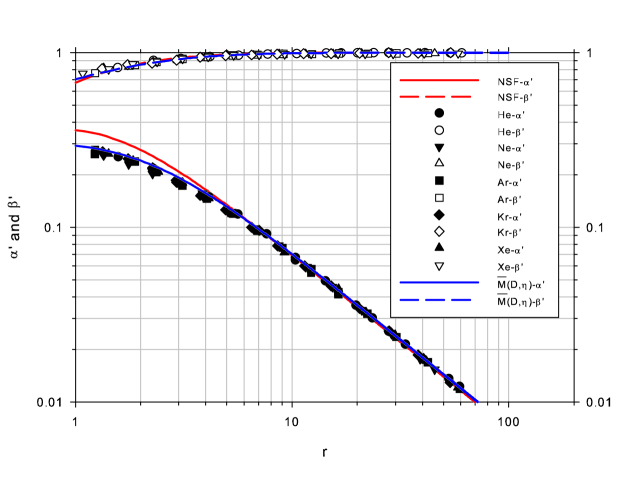
Figure 1: sound propagation in the noble gases

From figure 1, it is clear that my theory’s sound predictions match those of the NSF formulation in the hydrodynamic (high $r$, or low $K\!n$) regime, as intended.  As I have emphasized throughout, the $\overline{M}\left(D,\eta\right)$-formulation is a continuum theory appropriate for the $K\!n\ll 1$ regime, and so I make no general claims that it works well into more rarefied higher Knudsen number regimes.  However, figure 1 provides an intriguing demonstration that for this problem, it does significantly better than Navier-Stokes-Fourier there.  Of course, until I can provide a formal explanation, this should be viewed as strictly fortuitous.

In [24], I will use Green’s functions to solve the linearized general $\overline{M}$- formulation in order to fully describe planar sound waves emanating from a sinusoidally vibrating source into a fluid occupying infinite space. Afterwards, I will use this solution to interpret the sound roots in a more precise physical manner and relate them to the quantities that are measured in sound attenuation experiments such as Greenspan’s.

6 Sound at a Boundary

Morse and Ingard [28, Ch. 6] use the NSF equations in order to study low amplitude sound waves hitting a wall.  For easier comparison with their treatment and for general convenience, as well, let us use the thermodynamic relationships (293) and (294) to recast the $\overline{M}\left(D,\eta\right)$-formulation (1)/(4)–assuming variation is in the $x_{1}\equiv x$ direction only, $v_{1}\equiv v$ is the only non-zero component of the velocity, and there are no body forces–in terms of the variables, $\overline{m}$, $P$, $v$, and $T$, and then linearize about the constant equilibrium state,

$$\left(\overline{m},P,v,T\right)=\left(m_{\text{eq}},P_{\text{eq}},0,T_{\text{eq}}\right),$$ (91)

via

$$\overline{m} =m_{\text{eq}}+\delta\!\overline{m}$$ (92)

$$P =P_{\text{eq}}+\delta\!P$$ (93)

$$v =\delta\!v$$ (94)

$$T =T_{\text{eq}}+\delta\!T.$$ (95)

Assuming

$$\left|\delta\!\overline{m}\right| \ll m_{\text{eq}}$$

$$\left|\delta\!P\right| \ll P_{\text{eq}}$$ (96)

$$\left|\delta\!T\right| \ll T_{\text{eq}}$$

$$\left|\delta\!v\right| \ll c_{\text{eq}},$$

one obtains the following approximate system:

$$\frac{\partial\delta\!\overline{m}}{\partial t} =-m_{\text{eq}}\frac{\partial\delta\!v}{\partial x}$$ (97)

$$\frac{\partial\delta\!P}{\partial t} =D_{\text{eq}}\frac{\partial^{2}\delta\!P}{\partial x^{2}}-\left(mc^{2}\right)_{\text{eq}}\frac{\partial\delta\!v}{\partial x}$$ (98)

$$\frac{\partial\delta\!v}{\partial t} =-\frac{1}{m_{\text{eq}}}\frac{\partial\delta\!P}{\partial x}+D_{\text{eq}}\frac{\partial^{2}\delta\!v}{\partial x^{2}}$$ (99)

$$\frac{\partial\delta\!T}{\partial t} =D_{\text{eq}}\frac{\partial^{2}\delta\!T}{\partial x^{2}}-\left(\frac{T\alpha_{P}c^{2}}{c_{P}}\right)_{\text{eq}}\frac{\partial\delta\!v}{\partial x},$$ (100)

where $c_{P}$ is the isobaric specific heat.  Again, we see that the mechanical mass equation (97) may be uncoupled from the rest of the system, and postulating a solution

$$\left[\begin{array}[c]{c}\delta\!P\\ \delta\!v\\ \delta\!T\end{array}\right]$$

to the remaining system (98)-(100) that is proportional to

$$\exp\left(\kappa x+i\omega t\right)$$

with $\omega$ real and $\kappa$ complex, unsurprisingly leads to the same dispersion relation (65) and the same six roots (66)-(68) as before.  However, when my equations are cast in the present form, one notes the following interesting fact: the temperature equation (100) may be uncoupled from the pressure and velocity equations, so that the dispersion relation arising from the reduced system, (98) and (99), yields only the propagational roots (66) and the source roots (68).  The thermal roots (67) arise only when the temperature equation (100) is coupled back into the system.  This means that within the $\overline{M}\left(D,\eta\right)$-formulation, thermal modes of the solution may contribute only to the temperature variable and not the pressure or velocity variables, i.e. the mechanical variables.  On the other hand, propagational and source modes may contribute to all three.

Next, let us examine the length scales associated with each of these three types of roots.  If we compute the length scale as the distance it takes for a mode to attenuate to $1/e$ of its amplitude, then we find the propagational, thermal, and source mode lengths to be

$$l_{p}\equiv\frac{1}{\left|\operatorname{Re}\kappa_{p\left(\pm\right)}\right|}=\frac{1}{4\pi^{2}f^{2}}\left(\frac{c^{3}}{D}\right)_{\text{eq}},$$ (101)

$$l_{t}\equiv\frac{1}{\left|\operatorname{Re}\kappa_{t\left(\pm\right)}\right|}=\sqrt{\frac{D_{\text{eq}}}{\pi f}},$$ (102)

and

$$l_{s}\equiv\frac{1}{\left|\operatorname{Re}\kappa_{s\left(\pm\right)}\right|}=\left(\frac{D}{c}\right)_{\text{eq}},$$ (103)

respectively, where (66)-(68) and (70) have been used in the above.  For example, if we consider ultrasonic waves at frequency $f=11$ MHz as in Greenspan [14] and argon gas at normal temperature and pressure ($T_{\text{eq}}=300$ K and $P_{\text{eq}}=1.013\times 10^{5}$ Pa) with $D_{\text{eq}}=1.64\times 10^{-5}$ m²/s  (see appendix C) and $c_{\text{eq}}=323$ m/s from the classical monatomic ideal gas formula (307), then the above length scales are computed to be

$$l_{p}=4.30\times 10^{-4}\text{ m,}$$

$$l_{t}=6.87\times 10^{-7}\text{ m,}$$

and

$$l_{s}=5.08\times 10^{-8}\text{ m.}$$

In this case–and in general, for all ideal gases in the hydrodynamic regime–the source mode has a length scale $l_{s}$ roughly equal to the mean free path length of the gas in its equilibrium state $\left(T_{\text{eq}},P_{\text{eq}}\right)$, regardless of sound frequency, and

$$l_{p}\gg l_{t}>l_{s}.$$ (104)

Away from boundaries, the propagational modes of sound waves dominate.  However, depending on the boundary conditions, the thermal and source modes may play an important role near walls, causing the formation of boundary layers with lengths $l_{t}$ and $l_{s}$, respectively.

When the NSF equations (5)/(6) are recast using (293) and (294) and linearized as above, we arrive at the following system:

$$\frac{\partial\delta\!P}{\partial t} =\left(\frac{\alpha_{P}c^{2}k_{F}}{c_{P}}\right)_{\text{eq}}\frac{\partial^{2}\delta\!T}{\partial x^{2}}-\left(mc^{2}\right)_{\text{eq}}\frac{\partial\delta\!v}{\partial x}$$ (105)

$$\frac{\partial\delta\!v}{\partial t} =-\frac{1}{m_{\text{eq}}}\frac{\partial\delta\!P}{\partial x}+\left(\frac{\zeta_{NS}}{m}+\frac{4}{3}\frac{\eta}{m}\right)_{\text{eq}}\frac{\partial^{2}\delta\!v}{\partial x^{2}}$$ (106)

$$\frac{\partial\delta\!T}{\partial t} =\left(\frac{\gamma k_{F}}{mc_{P}}\right)_{\text{eq}}\frac{\partial^{2}\delta\!T}{\partial x^{2}}-\left(\frac{T\alpha_{P}c^{2}}{c_{P}}\right)_{\text{eq}}\frac{\partial\delta\!v}{\partial x},$$ (107)

which again yields dispersion relation (72) and the four roots (73) and (74).  Unlike in the $\overline{M}\left(D,\eta\right)$-formulation, none of the above equations uncouple from one another.  Therefore, in the NSF formulation the two possible modes, propagational and thermal, may contribute to each of the three variables: pressure, velocity, and temperature.

Using (73) and (74), the length scales associated with the propagational and thermal modes of the NSF formulation are computed to be

$$l_{p}\equiv\frac{1}{\left|\operatorname{Re}\kappa_{p\left(\pm\right)}\right|}=\frac{c_{\text{eq}}^{3}}{4\pi^{2}f^{2}\Gamma_{\text{eq}}}$$ (108)

and

$$l_{t}\equiv\frac{1}{\left|\operatorname{Re}\kappa_{t\left(\pm\right)}\right|}=\sqrt{\frac{\Sigma_{\text{eq}}}{\pi f}}\frac{1}{1-2\pi f\left(\frac{\Omega}{c^{2}}\right)_{\text{eq}}}.$$ (109)

In view of (77), equation (108) yields the same propagation length as (101).  Also, in the hydrodynamic regime, the thermal length given by (109) is the same order of magnitude as the thermal length (102) from my formulation.

Let us assume the $yz$-plane forms a sound barrier at $x=0$ for sound waves coming from the $+x$-direction and, as in Morse and Ingard, define the acoustic impedance of the wall as

$$z_{w}\equiv\frac{\text{acoustic pressure at wall}}{\text{normal fluid velocity at wall}}=-\left.\frac{\delta\!P}{\delta\!v}\right|_{x=0}.$$ (110)

Infinite impedance corresponds to a perfectly reflected sound wave in which its outgoing velocity is equal in magnitude and opposite in direction to its incoming velocity, resulting in

$$\left.\delta\!v\right|_{x=0}=0.$$ (111)

For non-infinite wall impedances, however, there is a non-zero normal fluid velocity at the wall.  Using the $\overline{M}\left(D,\eta\right)$-formulation, we may still consider the wall to be both stationary and impermeable by enforcing the no total mass flux condition,

$$\left.\underline{j}_{M}\cdot\underline{n}\right|_{x=0}=0$$ (112)

where, in this case, the normal vector $\underline{n}$ is the unit vector in the $-x$ direction.  With (9)/(4 a) linearized and thermodynamic relation (294), the above condition implies

$$\left.\left\{-D_{\text{eq}}\left[\begin{array}[c]{c}-\left(m\alpha_{P}\right)_{\text{eq}}\frac{\delta\!T}{dx}+\\ \left(\frac{\gamma}{c^{2}}\right)_{\text{eq}}\frac{\delta\!P}{dx}\end{array}\right]+m_{\text{eq}}\delta\!v\right\}\right|_{x=0}=0.$$ (113)

On the other hand, if (111) is not satisfied in the NSF formulation, there arises the curious situation of a non-zero normal mass flux at $x=0$.  Morse and Ingard [28, p. 260] explain this phenomenon as follows: ”The acoustic pressure acts on the surface and tends to make it move, or else tends to force more fluid into the pores of the surface.”  Wall movement and/or fluid lost to pores in the wall are yet never treated explicitly.

I will make the above ideas precise in a future paper [26] in which Green’s functions on a semi-infinite domain are used to solve linearized one-dimensional problems involving fluid disturbances interacting with an impedance wall.

7 Hydrodynamical Fluctuations

The procedure for investigating stationary-Gaussian-Markov processes, as described by Fox and Uhlenbeck [12], may be used to derive the formulas of hydrodynamical fluctuations for the $\overline{M}\left(D,\eta\right)$-formulation.  This involves using the linearized three-dimensional Cartesian version of the hydrodynamic equations (I.59) with transport coefficients given by (I.67), (I.68), and (I.61 b), interpreting the variables as stochastically fluctuating variables, and introducing zero-mean fluctuating hydrodynamic forces.  This yields the following Langevin type of system:

$$\frac{\partial\delta\!m}{\partial t} =D_{\text{eq}}\nabla^{2}\delta\!m-\nabla\cdot\delta\!\underline{p}-\nabla\cdot\underline{J}_{M}$$

$$\frac{\partial\delta\!\underline{p}}{\partial t} =\left[\begin{array}[c]{c}\left(\beta_{m}\right)_{\text{eq}}\nabla\delta\!m+\left(\beta_{u}\right)_{\text{eq}}\nabla\delta\!u+\\ \left(\frac{\eta}{m}\right)_{\text{eq}}\nabla^{2}\delta\!\underline{p}+\\ \left(D-\frac{\eta}{m}\right)_{\text{eq}}\nabla\left(\nabla\cdot\delta\!\underline{p}\right)\end{array}\right]-\nabla\cdot\underline{\underline{J}}_{\underline{P}}$$ (117)

$$\frac{\partial\delta\!u}{\partial t} =D_{\text{eq}}\nabla^{2}\delta\!u-\left(h_{M}\right)_{\text{eq}}\nabla\cdot\delta\!\underline{p}-\nabla\cdot\underline{J}_{U}.$$

In the above, the mechanical mass density equation has been uncoupled.  Also, $\underline{J}_{M}$, $\underline{\underline{J}}_{\underline{P}}$, and $\underline{J}_{U}$ represent the fluctuating mass, momentum, and internal energy fluxes, respectively, with $\underline{\underline{J}}_{\underline{P}}$ assumed to be symmetric and

$$\left\langle\underline{J}_{M}\right\rangle=\left\langle\underline{J}_{U}\right\rangle=\underline{0}\text{ and }\left\langle\underline{\underline{J}}_{\underline{P}}\right\rangle=\underline{\underline{0}},$$ (118)

where $\left\langle\_\right\rangle$ denotes a stochastic average.

Following the steps outlined in Fox and Uhlenbeck leads to a generalized fluctuation-dissipation theorem for stationary-Gaussian-Markov processes which, when expressed for the problem at hand, yields the following correlation formulas for the Cartesian components of the fluctuating fluxes:

$$\left\langle\left(J_{M}\right)_{i}\left(\underline{x},t\right)\left(J_{M}\right)_{j}\left(\underline{x}^{\prime},t^{\prime}\right)\right\rangle=$$

$$2V\left\langle\delta\!m^{2}\right\rangle_{V,\text{eq}}D_{\text{eq}}\delta\left(\underline{x}-\underline{x}^{\prime}\right)\delta\left(t-t^{\prime}\right)\delta_{ij},$$ (119)

$$\left\langle\left(J_{U}\right)_{i}\left(\underline{x},t\right)\left(J_{U}\right)_{j}\left(\underline{x}^{\prime},t^{\prime}\right)\right\rangle=$$

$$2V\left\langle\delta\!u^{2}\right\rangle_{V,\text{eq}}D_{\text{eq}}\delta\left(\underline{x}-\underline{x}^{\prime}\right)\delta\left(t-t^{\prime}\right)\delta_{ij},$$ (120)

$$\left\langle\left(J_{M}\right)_{i}\left(\underline{x},t\right)\left(J_{U}\right)_{j}\left(\underline{x}^{\prime},t^{\prime}\right)\right\rangle=$$

$$2V\left\langle\delta\!m\delta\!u\right\rangle_{V,\text{eq}}D_{\text{eq}}\delta\left(\underline{x}-\underline{x}^{\prime}\right)\delta\left(t-t^{\prime}\right)\delta_{ij},$$ (121)

$$\left\langle\left(J_{\underline{P}}\right)_{ij}\left(\underline{x},t\right)\left(J_{\underline{P}}\right)_{kl}\left(\underline{x}^{\prime},t^{\prime}\right)\right\rangle=$$

$$\left\{\begin{array}[c]{l}2k_{B}\left(mTD\right)_{\text{eq}}\delta\left(\underline{x}-\underline{x}^{\prime}\right)\delta\left(t-t^{\prime}\right)\text{ if }i=j=k=l\\ 2k_{B}\left(T\eta\right)_{\text{eq}}\delta\left(\underline{x}-\underline{x}^{\prime}\right)\delta\left(t-t^{\prime}\right)\text{ if }i=k\text{, }j=l\text{, }i\neq j\\ 2k_{B}\left(T\eta\right)_{\text{eq}}\delta\left(\underline{x}-\underline{x}^{\prime}\right)\delta\left(t-t^{\prime}\right)\text{ if }i=l\text{, }j=k\text{, }i\neq j\\ 2k_{B}\left[T\left(mD-2\eta\right)\right]_{\text{eq}}\delta\left(\underline{x}-\underline{x}^{\prime}\right)\delta\left(t-t^{\prime}\right)\text{ if }\left(\begin{array}[c]{c}i=j\text{,}\\ k=l\text{,}\\ i\neq k\end{array}\right)\\ 0\text{ otherwise}\end{array}\right.,$$ (130)

and

$$\left\langle\left(J_{\underline{P}}\right)_{ij}\left(\underline{x},t\right)\left(J_{M}\right)_{k}\left(\underline{x}^{\prime},t^{\prime}\right)\right\rangle=\left\langle\left(J_{\underline{P}}\right)_{ij}\left(\underline{x},t\right)\left(J_{U}\right)_{k}\left(\underline{x}^{\prime},t^{\prime}\right)\right\rangle=0.$$ (131)

In the above formulas, the indices, $i$, $j$, and $k$, may equal $1$, $2$, or $3$ (the three Cartesian directions), $\delta$ is used to represent Dirac delta distributions, $\delta_{ij}$ is the Kronecker delta, $k_{B}$ denotes the Boltzmann constant, and I have employed equilibrium thermodynamic fluctuation formulas (296)-(298), which apply to a system of fixed volume $V$ in contact with a heat/particle reservoir.  Note the similarity in form of equations (119)-(121).

For comparison, the Langevin system corresponding to the NSF formulation is

$$\frac{\partial\delta\!m}{\partial t} =-\nabla\cdot\delta\!\underline{p}-\nabla\cdot\underline{J}_{M}$$

$$\frac{\partial\delta\!\underline{p}}{\partial t} =\left\{\begin{array}[c]{c}\left(\beta_{m}\right)_{\text{eq}}\nabla\delta\!m+\left(\beta_{u}\right)_{\text{eq}}\nabla\delta\!u+\\ \left(\frac{\eta}{m}\right)_{\text{eq}}\nabla^{2}\delta\!\underline{p}+\\ \left(\frac{\zeta_{NS}+\eta/3}{m}\right)_{\text{eq}}\nabla\left(\nabla\cdot\delta\!\underline{p}\right)\end{array}\right\}-\nabla\cdot\underline{\underline{J}}_{\underline{P}}$$ (135)

$$\frac{\partial\delta\!u}{\partial t} =\left\{\begin{array}[c]{c}\left(\frac{k_{F}}{mc_{V}}\right)_{\text{eq}}\nabla^{2}\delta\!u-\\ \left[\frac{\left(h_{M}-\frac{T\alpha_{P}}{m\kappa_{T}}\right)k_{F}}{mc_{V}}\right]_{\text{eq}}\nabla^{2}\delta\!m-\\ \left(h_{M}\right)_{\text{eq}}\nabla\cdot\delta\!\underline{p}\end{array}\right\}-\nabla\cdot\underline{J}_{U}$$ (139)

from which one may derive Fox and Uhlenbeck’s correlations,

$$\left\langle\left(J_{M}\right)_{i}\left(\underline{x},t\right)\left(J_{M}\right)_{j}\left(\underline{x}^{\prime},t^{\prime}\right)\right\rangle=0,$$ (140)

$$\left\langle\left(J_{U}\right)_{i}\left(\underline{x},t\right)\left(J_{U}\right)_{j}\left(\underline{x}^{\prime},t^{\prime}\right)\right\rangle=2k_{B}\left(T^{2}k_{F}\right)_{\text{eq}}\delta\left(\underline{x}-\underline{x}^{\prime}\right)\delta\left(t-t^{\prime}\right)\delta_{ij},$$ (141)

$$\left\langle\left(J_{M}\right)_{i}\left(\underline{x},t\right)\left(J_{U}\right)_{j}\left(\underline{x}^{\prime},t^{\prime}\right)\right\rangle=0,$$ (142)

$$\left\langle\left(J_{\underline{P}}\right)_{ij}\left(\underline{x},t\right)\left(J_{\underline{P}}\right)_{kl}\left(\underline{x}^{\prime},t^{\prime}\right)\right\rangle=$$

$$\left\{\begin{array}[c]{l}2k_{B}\left[T\left(\frac{4\eta}{3}+\zeta_{NS}\right)\right]_{\text{eq}}\delta\left(\underline{x}-\underline{x}^{\prime}\right)\delta\left(t-t^{\prime}\right)\text{ if }i=j=k=l\\ 2k_{B}\left(T\eta\right)_{\text{eq}}\delta\left(\underline{x}-\underline{x}^{\prime}\right)\delta\left(t-t^{\prime}\right)\text{ if }i=k\text{, }j=l\text{, }i\neq j\\ 2k_{B}\left(T\eta\right)_{\text{eq}}\delta\left(\underline{x}-\underline{x}^{\prime}\right)\delta\left(t-t^{\prime}\right)\text{ if }i=l\text{, }j=k\text{, }i\neq j\\ 2k_{B}\left[T\left(\zeta_{NS}-\frac{2\eta}{3}\right)\right]_{\text{eq}}\delta\left(\underline{x}-\underline{x}^{\prime}\right)\delta\left(t-t^{\prime}\right)\text{ if }\left(\begin{array}[c]{c}i=j\text{,}\\ k=l\text{,}\\ i\neq k\end{array}\right)\\ 0\text{ otherwise}\end{array}\right.,$$ (151)

and

$$\left\langle\left(J_{\underline{P}}\right)_{ij}\left(\underline{x},t\right)\left(J_{M}\right)_{k}\left(\underline{x}^{\prime},t^{\prime}\right)\right\rangle=\left\langle\left(J_{\underline{P}}\right)_{ij}\left(\underline{x},t\right)\left(J_{U}\right)_{k}\left(\underline{x}^{\prime},t^{\prime}\right)\right\rangle=0.$$ (152)

Therefore, in the NSF formulation,

$$\underline{J}_{M}=\underline{0},$$ (153)

whereas my theory predicts a non-zero fluctuating mass flux.

This exercise illuminates certain ideas about the thermodynamic nature of a continuum mechanical point, i.e. a point occupied by matter whose motion is tracked by its local velocity, $\underline{v}$, and whose infinitesimal volume is determined by its continuum mechanical deformation.  As per the local equilibrium hypothesis, near-equilibrium continuum theories are constructed under the assumption that any given continuum mechanical point may be viewed as an equilibrium thermodynamic subsystem in contact with the rest of the material which acts as a reservoir.  The question as to whether or not the fluctuating mass flux $\underline{J}_{M}$ is zero, decides the very nature of this reservoir.  All continuum theories view the surrounding material as a reservoir for heat (so that the point exchanges energy with the surrounding fluid to maintain a temperature determined by thermodynamics), but is it also a particle reservoir (so that it exchanges mass with the surrounding fluid to maintain a thermodynamically determined chemical potential)?  My theory, with its non-zero $\underline{J}_{M}$, asserts that it is, whereas the Navier-Stokes-Fourier theory, in view of its (153) prediction, argues that it is not, meaning that each continuum mechanical point should be conceived of as having an impermeable wall surrounding it.  Although subsystems and reservoirs are abstract constructs in this setting, I believe that it makes sense to allow the mass of a continuum mechanical point to fluctuate.  This view is reinforced by the natural appearance of fluctuation formulas (296)-(298) for a heat/particle reservoir in my theory’s correlations, (119)-(121).

8 Light Scattering

One may derive hydrodynamic light scattering spectra for the $\overline{M}\left(D,\eta\right)$- formulation by using the same procedure as that used in Berne and Pecora [2, §10.4] for the NSF formulation.  The main steps involved are to (1) linearize the Cartesian three-dimensional equations–expressed in terms of the variables, mechanical mass $\overline{m}$, particle number density $n_{p}=N_{A}m/A$ where $N_{A}$ and $A$ respectively denote Avogadro’s number and the atomic weight, divergence of the velocity $\phi=\nabla\cdot\underline{v}$, and temperature $T$–about the constant equilibrium state,

$$\left(\overline{m},n_{p},\phi,T\right)=\left(m_{\text{eq}},\left(n_{p}\right)_{\text{eq}},0,T_{\text{eq}}\right),$$ (154)

(2) uncouple the mechanical mass density equation, (3) take the Fourier-Laplace transform of the remaining linear system, (4) solve for the Fourier-Laplace transformed variables, and (5) use this solution to construct time-correlation functions and their spectral densities.  Of particular interest is the particle-particle spectrum, computed for my formulation to be exactly

$$S_{N_{p}N_{p}}\left(k,\omega\right)=\frac{\mathcal{S}}{\pi}\left(\begin{array}[c]{c}\left(1-\frac{1}{\gamma_{\text{eq}}}\right)\frac{D_{\text{eq}}k^{2}}{\omega^{2}+\left(D_{\text{eq}}k^{2}\right)^{2}}+\\ \frac{1}{2\gamma_{\text{eq}}}\left\{\begin{array}[c]{c}\frac{D_{\text{eq}}k^{2}}{\left[\omega+\omega_{B}\left(k\right)\right]^{2}+\left(D_{\text{eq}}k^{2}\right)^{2}}+\\ \frac{D_{\text{eq}}k^{2}}{\left[\omega-\omega_{B}\left(k\right)\right]^{2}+\left(D_{\text{eq}}k^{2}\right)^{2}}\end{array}\right\}\end{array}\right).$$ (155)

In the above, $k$ is used to represent the magnitude of the wave vector, $\underline{k}$; $\omega$ is the angular frequency; $\mathcal{S}$ is the structure factor defined as

$$\mathcal{S} =\left\langle\delta\!N_{p}^{2}\right\rangle_{V,\text{eq}}$$ (156)

$$=Vk_{B}\left(n_{p}^{2}T\kappa_{T}\right)_{\text{eq}}$$ (157)

by equation (299) in appendix B where $V$ represents the scattering volume; and $\omega_{B}\left(k\right)$ is the frequency shift of the Brillouin doublets,

$$\omega_{B}\left(k\right)=c_{\text{eq}}k.$$ (158)

The right-hand side of (155) is the sum of three Lorentzian line shapes, the first of which is the central Rayleigh peak, and the other two, the negatively and positively $\omega_{B}\left(k\right)$-shifted Brillouin peaks.  The Brillouin peaks represent light scattering due to the sound modes, or phonons, generated by pressure fluctuations, and the Rayleigh peak is caused by light being scattered from specific entropy fluctuations.

The NSF particle-particle spectrum is given by the more complicated expression,

$$S_{N_{p}N_{p}}\left(k,\omega\right)=$$

$$\frac{\mathcal{S}}{\pi}\operatorname{Re}\left(\frac{\left\{\begin{array}[c]{c}-\omega^{2}+i\omega\left[\frac{\zeta_{NS}}{m}+\left(\frac{4}{3}+E\!u\right)\frac{\eta}{m}\right]_{\text{eq}}k^{2}+\\ \left(1-\frac{1}{\gamma_{\text{eq}}}\right)\omega_{B}^{2}\left(k\right)+\\ \left[E\!u\left(\frac{\zeta_{NS}}{m}+\frac{4}{3}\frac{\eta}{m}\right)\frac{\eta}{m}\right]_{\text{eq}}k^{4}\end{array}\right\}}{\left\{\begin{array}[c]{c}-i\omega^{3}-\omega^{2}\left[\frac{\zeta_{NS}}{m}+\left(\frac{4}{3}+E\!u\right)\frac{\eta}{m}\right]_{\text{eq}}k^{2}+\\ i\omega\left\{\omega_{B}^{2}\left(k\right)+\left[E\!u\left(\frac{\zeta_{NS}}{m}+\frac{4}{3}\frac{\eta}{m}\right)\frac{\eta}{m}\right]_{\text{eq}}k^{4}\right\}+\\ \left(\frac{E\!u}{\gamma}\frac{\eta}{m}\right)_{\text{eq}}\omega_{B}^{2}\left(k\right)k^{2}\end{array}\right\}}\right),$$ (165)

where $E\!u$ is the Euken ratio defined in (41).  In the hydrodynamic regime for which

$$\left(\frac{\eta}{mc}\right)_{\text{eq}}k\ll 1,$$ (166)

equation (165) becomes approximately

$$S_{N_{p}N_{p}}\left(k,\omega\right)=$$

$$\frac{\mathcal{S}}{\pi}\left(\begin{array}[c]{c}\left(1-\frac{1}{\gamma_{\text{eq}}}\right)\frac{\Sigma_{\text{eq}}k^{2}}{\omega^{2}+\left(\Sigma_{\text{eq}}k^{2}\right)^{2}}+\\ \frac{1}{2\gamma_{\text{eq}}}\left\{\frac{\Gamma_{\text{eq}}k^{2}}{\left[\omega+\omega_{B}\left(k\right)\right]^{2}+\left(\Gamma_{\text{eq}}k^{2}\right)^{2}}+\frac{\Gamma_{\text{eq}}k^{2}}{\left[\omega-\omega_{B}\left(k\right)\right]^{2}+\left(\Gamma_{\text{eq}}k^{2}\right)^{2}}\right\}+\\ \frac{b\left(k\right)}{2}\left\{\frac{\left[\omega+\omega\left(k\right)\right]}{\left[\omega+\omega_{B}\left(k\right)\right]^{2}+\left(\Gamma_{\text{eq}}k^{2}\right)^{2}}-\frac{\left[\omega-\omega\left(k\right)\right]}{\left[\omega-\omega_{B}\left(k\right)\right]^{2}+\left(\Gamma_{\text{eq}}k^{2}\right)^{2}}\right\}\end{array}\right),$$ (170)

where $\Sigma$ and $\Gamma$ are defined in (42) and (43) and

$$b\left(k\right)\equiv\frac{k^{2}}{\gamma_{\text{eq}}\omega_{B}\left(k\right)}\left\{\frac{\zeta_{NS}}{2m}+\left[\frac{3}{2}\left(1-\frac{1}{\gamma}\right)E\!u+\frac{2}{3}\right]\frac{\eta}{m}\right\}_{\text{eq}}.$$ (171)

In approximate expression (170), the first three terms represent the Lorentzian Rayleigh and Brillouin peaks and the last two terms give a fairly small, but not negligible, non-Lorentzian contribution.

Next, as in Clark [7] and Fookson et al. [13], let us define a dimensionless angular frequency,

$$\text{x}=\left(\frac{1}{c}\sqrt{\frac{\gamma}{2}}\right)_{\text{eq}}\frac{\omega}{k},$$ (172)

the dimensionless uniformity parameter,

$$\text{y}=\frac{1}{3k}\left(\sqrt{\frac{2}{\gamma}}\frac{mc}{\eta}\right)_{\text{eq}},$$ (173)

which is inversely proportional to the Knudsen number for a gas, and the dimensionless particle-particle spectrum,

$$S_{N_{p}N_{p}}^{\prime}=\left(c\sqrt{\frac{2}{\gamma}}\right)_{\text{eq}}\frac{k}{\mathcal{S}}S_{N_{p}N_{p}},$$ (174)

which has an area of $1$ when written as a function of x and y and integrated over all x.  Figure 2 is a plot of the dimensionless particle-particle spectra, $S_{N_{p}N_{p}}^{\prime}\left(\text{x},\text{y}\right)$, predicted by the $\overline{M}\left(D,\eta\right)$-formulation (blue) and the NSF formulation (red) for a classical monatomic ideal gas with y $=20$ and equations (78), (79), and (307) assumed.  The arrows indicate the widths at half-height.  (Since the spectra are symmetric about the $0$ frequency, only the right Brillouin peaks are shown.)

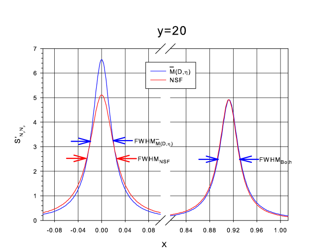
Figure 2: theoretical light scattering spectra for a classical monatomic ideal gas (y $=20$)

Both theories predict similar Brillouin peaks, but the $\overline{M}\left(D,\eta\right)$-formulation has a Rayleigh peak with a maximum about $29\%$ higher and width at half-height about $29\%$ narrower than that of NSF.  On the other hand, the areas under both of the Rayleigh peak predictions are the same, leading to identical Landau-Placzek ratios, i.e.

$$\frac{\text{area of (central) Rayleigh peak}}{\text{area of both (shifted) Brillouin peaks}}=\gamma_{\text{eq}}-1$$ (175)

which, in view of (306) for a classical monatomic ideal gas, is $2/3$.  Note that for the $\overline{M}\left(D,\eta\right)$-formulation, the Brillouin peaks and the Rayleigh peak all have the same width at half-height, a quantity that is inversely proportional to the lifetime of the excitation corresponding to the peak.  This means that my theory predicts the same lifetime for phonons as it does for excitations caused by specific entropy fluctuations, whereas the NSF formulation predicts that excitations caused by specific entropy fluctuations die out sooner than the phonons ($29\%$ sooner in the case of a classical monatomic ideal gas).  One other thing to note is that the Brillouin portion of my exact spectrum (155) predicts phonons corresponding exactly to the adiabatic sound speed, $c_{\text{eq}}$, whereas the approximate Navier-Stokes-Fourier spectrum (170) predicts a small change in speed due to the non-Lorentzian contributions, e.g. in figure 2, it can be observed that for a classical monatomic ideal gas, there is a shift of the NSF Brillouin peaks slightly toward the center frequency.

9 The Effect of Gravity on the Atmosphere

Let us limit our investigation to the lowest part of the Earth’s atmosphere, the troposphere.  Typical discussions of this problem–see Sommerfeld [31, ch. II §7 pp. 49-55]–do not involve the equations of fluid dynamics and I briefly summarize the ideas behind this type of treatment first.  One begins with the hydrostatic equation for the pressure as a function of altitude,

$$P\left(x\right)=P_{\text{sl}}-m_{\text{sl}}gx$$ (176)

where $x$ is the altitude above sea level, a subscript of ”sl” indicates values for air at sea level, and $g$ is the constant acceleration of gravity, which acts in the $-x$-direction.  For a classical ideal gas, relationship (300) allows us to write (176) as

$$P\left(x\right)=P_{\text{sl}}-\frac{A}{R}\left(\frac{P}{T}\right)_{\text{sl}}gx.$$ (177)

Next, one makes the observation that, in the troposphere, like the pressure, the temperature also decreases with altitude.  Furthermore, one obtains this behavior qualitatively by enforcing the isentropic assumption,

$$\frac{d\sigma}{dx}=0,$$ (178)

where $\sigma$ represents the specific entropy.  Using relation (305) for a classical ideal gas with constant specific heat, one finds the approximation,

$$\frac{d\sigma}{dx}=\frac{R\gamma}{A\left(\gamma-1\right)T_{\text{sl}}}\frac{dT}{dx}-\frac{R}{AP_{\text{sl}}}\frac{dP}{dx},$$ (179)

holds when $x$ is not too high above sea level, and this relationship, when used together with (177), implies

$$\frac{dT}{dx}=-\frac{A\left(\gamma-1\right)}{R\gamma}g$$ (180)

so that the temperature as a function of altitude is given by

$$T\left(x\right)=T_{\text{sl}}-\frac{A\left(\gamma-1\right)}{R\gamma}gx.$$ (181)

Using the values $g=9.81$ m$/$s², $R=8.31$ J/$\left(\text{mol}\cdot\text{K}\right)$, and the atomic weight and ratio of specific heats for dry air, $A=0.0290$ kg/m³ and $\gamma=1.4$, the quantity $-dT/dx$, called the temperature lapse rate, is calculated to be

$$-\frac{dT}{dx}=0.0098\text{ K/m,}$$ (182)

which is high when compared to the average measured value presented in [39]:

$$-\frac{dT}{dx}=0.0065\text{ K/m,}$$ (183)

although these being the same order of magnitude is somewhat of a triumph in view of all of the simplifying assumptions made in order to obtain (182).

As mentioned earlier, the equations of fluid dynamics are not used at all in the above arguments.  Let us also point out that the isentropic assumption was chosen because it gives a temperature law which predicts nature better than, say, an isothermal assumption does, and it was not, in fact, derived from other principles.  Below, I treat this problem using the linearized steady-state equations of fluid dynamics with mass and total energy balance considerations, and I show that the $\overline{M}\left(D,\eta\right)$-formulation predicts the isentropic condition (178), whereas–under the same assumptions–the NSF formulation predicts an unphysical isothermal condition.

We once again have a Cartesian one-dimensional problem with variation in the $x_{1}\equiv x$ direction only, and $v_{1}\equiv v$ as the only non-zero velocity component.  For this steady-state problem it is appropriate to use $\overline{M}\left(D,\eta\right)$-formulation (15) with the linearization performed about the constant state,

$$\left(\overline{m},P,v,T\right)=\left(m_{\text{sl}},P_{\text{sl}},0,T_{\text{sl}}\right).$$ (184)

Taking the linearized gravitational force to be

$$\overline{m}\left(f_{\overline{M}}\right)_{1}=-m_{\text{sl}}g,$$ (185)

one obtains

$$0 =\frac{dv}{dx}$$

$$0 =\frac{d^{2}P}{dx^{2}}$$ (186)

$$0 =-\frac{dP}{dx}+\eta_{\text{sl}}\frac{d^{2}v}{dx^{2}}-m_{\text{sl}}g$$

$$0 =\frac{d^{2}T}{dx^{2}}.$$

We solve these equations with the boundary conditions,

$$P\left(0\right)=P_{\text{sl}}\text{ and }T\left(0\right)=T_{\text{sl}},$$ (187)

to find

$$v\left(x\right) =\mathcal{C}_{1}$$

$$P\left(x\right) =P_{\text{sl}}-m_{\text{sl}}gx$$ (188)

$$T\left(x\right) =T_{\text{sl}}+\mathcal{C}_{2}x,$$

where (188 b) is the hydrostatic equation (176), and the $\mathcal{C}$’s are constants we must find using extra constraints.  The $\overline{M}\left(D,\eta\right)$-formulation flux equations (16) and (17) for this one-dimensional problem become

$$\left(j_{E}\right)_{1}=-D_{\text{sl}}\left\{\begin{array}[c]{c}\left[m\left(c_{P}-h_{M}\alpha_{P}\right)\right]_{\text{sl}}\frac{dT}{dx}+\\ \left(\frac{h_{M}\gamma}{c^{2}}-T\alpha_{P}\right)_{\text{sl}}\frac{dP}{dx}\end{array}\right\}+\left(mh_{M}\right)_{\text{sl}}v$$ (189)

and

$$\left(j_{M}\right)_{1}=-D_{\text{sl}}\left[-\left(m\alpha_{P}\right)_{\text{sl}}\frac{dT}{dx}+\left(\frac{\gamma}{c^{2}}\right)_{\text{sl}}\frac{dP}{dx}\right]+m_{\text{sl}}v.$$ (190)

It makes physical sense to enforce the constraints that there are no mass or total energy flux through the atmosphere due to gravity:

$$\left(j_{E}\right)_{1}=\left(j_{M}\right)_{1}=0.$$ (191)

Therefore, using (189) and (190) together with solution (188), these constraints imply

$$0 =-D_{\text{sl}}\left\{\begin{array}[c]{c}\left[m\left(c_{P}-h_{M}\alpha_{P}\right)\right]_{\text{sl}}\mathcal{C}_{2}-\\ \left(\frac{h_{M}\gamma}{c^{2}}-T\alpha_{P}\right)_{\text{sl}}m_{\text{sl}}g\end{array}\right\}+\left(mh_{M}\right)_{\text{sl}}\mathcal{C}_{1}$$ (194)

$$0 =-D_{\text{sl}}\left[-\left(m\alpha_{P}\right)_{\text{sl}}\mathcal{C}_{2}-\left(\frac{\gamma}{c^{2}}\right)_{\text{sl}}m_{\text{sl}}g\right]+m_{\text{sl}}\mathcal{C}_{1}$$

which, when solved simultaneously for the two constants, gives

$$\mathcal{C}_{1}=-g\left(\frac{D}{c^{2}}\right)_{\text{sl}}\text{ and }\mathcal{C}_{2}=-\left(\frac{T\alpha_{P}}{c_{P}}\right)_{\text{sl}}g,$$ (195)

where I have used thermodynamic relationship (290) to write (195 a).  Thus, solution (188) becomes

$$v\left(x\right) =-g\left(\frac{D}{c^{2}}\right)_{\text{sl}}$$

$$P\left(x\right) =P_{\text{sl}}-m_{\text{sl}}gx$$ (196)

$$T\left(x\right) =T_{\text{sl}}-\left(\frac{T\alpha_{P}}{c_{P}}\right)_{\text{sl}}gx.$$

Note the following: (1) thermodynamic relationship (295) implies

$$\frac{d\sigma}{dx}=\left(\frac{c_{P}}{T}\right)_{\text{sl}}\frac{dT}{dx}-\left(\frac{\alpha_{P}}{m}\right)_{\text{sl}}\frac{dP}{dx}$$ (197)

and when (196 b and c) are used in the right-hand side, this yields the isentropic condition (178), (2) when classical ideal gas relationships (301) and (303) are used in (196 c), one finds the temperature lapse rate to be the same as the one predicted by equation (180), and (3) using the estimates $c_{\text{sl}}=340$ m/s and $D_{\text{sl}}=1.82\times 10^{-5}$ m²/s for air at sea level, the above equation predicts a very small constant velocity directed towards the Earth,

$$v=-1.54\times 10^{-9}\text{ m/s,}$$ (198)

which is analogous to the thermophoretic velocity treated in §11.

Solving steady-state NSF equations (18) linearized about state (184), with body force (185) and boundary conditions (187), one obtains the same form of solution as (188).  The flux equations (19) and (20) for this one-dimensional problem are

$$\left(j_{E}\right)_{1}=-\left(k_{F}\right)_{\text{sl}}\frac{dT}{dx}+\left(mh_{M}\right)_{\text{sl}}v$$ (199)

and

$$\left(j_{M}\right)_{1}=m_{\text{sl}}v,$$ (200)

and therefore we see that enforcing constraints (191) for no mass or total energy flux, gives rise to a zero velocity solution and an isothermal condition.

10 Poiseuille Flow

So far in this paper, I have neglected to study any examples that result in a non-zero rotational (divergence-free) part of the velocity, $\underline{v}_{R}$.  Therefore, let us now look at a basic example in which this part of the velocity arises: laminar Poiseuille flow through a cylinder, which is depicted schematically in figure 3.

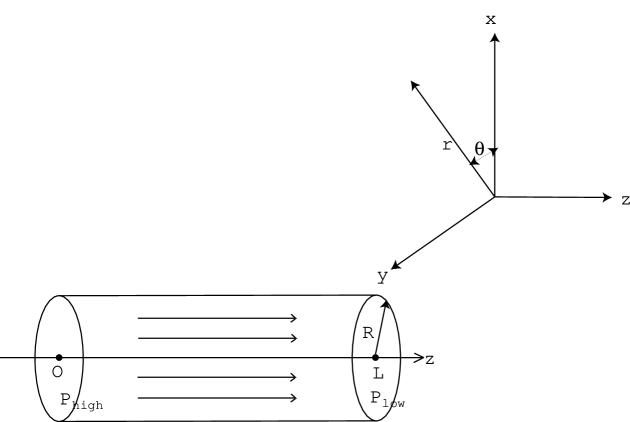
Figure 3: Poiseuille flow

Suppose that on the $z=0$ side, the fluid is maintained at a pressure $P_{\text{high}}$ and temperature $T_{\ast}$ and on the $z=L$ side with a lower pressure of $P_{\text{low}}$ and the same temperature $T_{\ast}$.  This, of course, causes steady-state flow in the $+z$-direction.  In addition, let us make the following assumptions: (1) the radius $\mathcal{R}$ of the cylinder is much larger than the mean free path length of the fluid so that $K\!n$ is small, (2) the length $L$ of the cylinder is quite a bit larger than the radius so that possible entrance and exit effects at the ends may be neglected , (3) the pressure gradient is small so that we may linearize, (4) parameters are chosen to yield a fairly small Reynolds number so that the flow is laminar (i.e. the radius and the pressure gradient cannot be too large and the shear viscosity cannot be too small), and (5) the cylinder itself has uniform temperature $T_{\ast}$.  It is clear that we can model this as a two-dimensional cylindrical problem in the $r$ and $z$ variables.

Let $P_{\ast}$ represent the average pressure,

$$P_{\ast}=\frac{P_{\text{high}}+P_{\text{low}}}{2}$$ (201)

and suppose everything with a subscript ”$\ast$” is evaluated at $\left(P_{\ast},T_{\ast}\right)$.  For this two-dimensional problem, the steady-state $\overline{M}\left(D,\eta\right)$-formulation (15) with the linearization performed about

$$\left(\overline{m},P,\underline{v},T\right)=\left(m_{\ast},P_{\ast},\underline{0},T_{\ast}\right),$$ (202)

is expressed–with the use of the cylindrical coordinate formulas presented in appendix A–as

$$0 =\frac{1}{r}\frac{\partial}{\partial r}\left(rv_{r}\right)+\frac{\partial v_{z}}{\partial z}$$

$$0 =\frac{1}{r}\frac{\partial}{\partial r}\left(r\frac{\partial P}{\partial r}\right)+\frac{\partial^{2}P}{\partial z^{2}}$$

$$0 =-\frac{\partial P}{\partial r}+\eta_{\ast}\left\{\frac{\partial}{\partial r}\left[\frac{1}{r}\frac{\partial}{\partial r}\left(rv_{r}\right)\right]+\frac{\partial^{2}v_{r}}{\partial z^{2}}\right\}$$ (203)

$$0 =-\frac{\partial P}{\partial z}+\eta_{\ast}\left[\frac{1}{r}\frac{\partial}{\partial r}\left(r\frac{\partial v_{z}}{\partial r}\right)+\frac{\partial^{2}v_{z}}{\partial z^{2}}\right]$$

$$0 =\frac{1}{r}\frac{\partial}{\partial r}\left(r\frac{\partial T}{\partial r}\right)+\frac{\partial^{2}T}{\partial z^{2}},$$

which we intend to solve with the following boundary conditions:

$$\left.P\right|_{z=0} =P_{\text{high}}$$ (204)

$$\left.P\right|_{z=L} =P_{\text{low}},$$ (205)

$$\left.T\right|_{z=0}=\left.T\right|_{z=L}=\left.T\right|_{r=\mathcal{R}}=T_{\ast},$$ (206)

the no-slip condition,

$$\left.v_{z}\right|_{r=\mathcal{R}}=0,$$ (207)

and the requirement that

$$\left.v_{z}\right|_{r=0}\text{ is finite.}$$ (208)

Immediately, we see that solving Laplace’s equation (203 e) with boundary conditions (206) for the temperature, yields the constant solution,

$$T=T_{\ast}.$$ (209)

With this fact and cylindrical coordinate formulas (276) and (278), one may express the $r$ and $z$ components of the $\overline{M}\left(D,\eta\right)$-formulation total energy and mass fluxes (16) and (17) as

$$\left(j_{E}\right)_{r} =-\left[D\left(\frac{h_{M}\gamma}{c^{2}}-T\alpha_{P}\right)\right]_{\ast}\frac{\partial P}{\partial r}+\left(mh_{M}\right)_{\ast}v_{r}$$ (210)

$$\left(j_{E}\right)_{z} =-\left[D\left(\frac{h_{M}\gamma}{c^{2}}-T\alpha_{P}\right)\right]_{\ast}\frac{\partial P}{\partial z}+\left(mh_{M}\right)_{\ast}v_{z}$$ (211)

and

$$\left(j_{M}\right)_{r} =-\left[D\left(\frac{\gamma}{c^{2}}\right)\right]_{\ast}\frac{\partial P}{\partial r}+m_{\ast}v_{r}$$ (212)

$$\left(j_{M}\right)_{z} =-\left[D\left(\frac{\gamma}{c^{2}}\right)\right]_{\ast}\frac{\partial P}{\partial z}+m_{\ast}v_{z}.$$ (213)

Next, one observes that for this steady-state problem to be physical, there must be no radial mass or total energy flux, i.e.

$$\left(j_{E}\right)_{r}=\left(j_{M}\right)_{r}=0$$ (214)

must be satisfied, which requires

$$\frac{\partial P}{\partial r}=0\text{ and }v_{r}=0.$$ (215)

Substituting (215) into equations (203 a-d) reduces them to

$$0 =\frac{\partial v_{z}}{\partial z}$$

$$0 =\frac{\partial^{2}P}{\partial z^{2}}$$ (216)

$$0 =-\frac{\partial P}{\partial z}+\eta_{\ast}\left[\frac{1}{r}\frac{\partial}{\partial r}\left(r\frac{\partial v_{z}}{\partial r}\right)+\frac{\partial^{2}v_{z}}{\partial z^{2}}\right],$$

and since (216 a) implies that $v_{z}$ is a function of $r$ only, we are left to solve

$$0 =\frac{\partial^{2}P}{\partial z^{2}}$$ (217)

$$0 =-\frac{\partial P}{\partial z}+\eta_{\ast}\left[\frac{1}{r}\frac{\partial}{\partial r}\left(r\frac{\partial v_{z}}{\partial r}\right)\right]$$ (218)

with boundary conditions (204), (205), (207), and (208).  Doing so, yields the familiar solution,

$$P\left(z\right) =P_{\text{high}}-\left(\frac{P_{\text{high}}-P_{\text{low}}}{L}\right)z$$ (219)

$$v_{z}\left(r\right) =\left(\frac{P_{\text{high}}-P_{\text{low}}}{4\eta_{\ast}L}\right)\left(\mathcal{R}^{2}-r^{2}\right),$$ (220)

which is the same as the one predicted by the NSF equations–see Bird, Stewart, and Lightfoot [3, pp. 48-52].  However, it is important to remark that in the NSF description, the linear equation (219) for the pressure is assumed rather than derived.

Next, the average velocity is computed as

$$\overline{v}_{z}=\frac{\int\nolimits_{0}^{2\pi}\int\nolimits_{0}^{\mathcal{R}}v_{z}\left(r\right)rdrd\theta}{\int\nolimits_{0}^{2\pi}\int\nolimits_{0}^{\mathcal{R}}rdrd\theta}$$ (221)

and the average convective mass flow rate as

$$\dot{M}_{\text{conv}}=\pi\mathcal{R}^{2}m_{\text{av}}\overline{v}_{z},$$ (222)

which evaluates to the familiar Hagen-Poiseuille formula predicted by the NSF equations,

$$\dot{M}_{\text{conv}}=\frac{\pi\mathcal{R}^{4}}{8}\left(\frac{m}{\eta}\right)_{\ast}\left(\frac{P_{\text{high}}-P_{\text{low}}}{L}\right),$$ (223)

when velocity profile (220) is used.  However, in the $\overline{M}\left(D,\eta\right)$-formulation, there is an additional diffusive contribution to the mass flow rate, given by

$$\dot{M}_{\text{dif}}=\pi\mathcal{R}^{2}\left(q_{M}\right)_{z},$$ (224)

where the non-convective mass flux $\left(q_{M}\right)_{z}$ is found by subtracting the convective part from (213) and using pressure equation (219), which yields

$$\dot{M}_{\text{dif}}=\pi\mathcal{R}^{2}\left(\frac{D\gamma}{c^{2}}\right)_{\ast}\left(\frac{P_{\text{high}}-P_{\text{low}}}{L}\right).$$ (225)

The total mass flow rate for the $\overline{M}\left(D,\eta\right)$-formulation is then the sum of the convective and diffusive parts:

$$\dot{M}=\left(\frac{P_{\text{high}}-P_{\text{low}}}{L}\right)\pi\mathcal{R}^{2}\left[\frac{\mathcal{R}^{2}}{8}\left(\frac{m}{\eta}\right)_{\ast}+\left(\frac{D\gamma}{c^{2}}\right)_{\ast}\right].$$ (226)

Note that under the assumptions given at the beginning of this section the diffusive part is very small compared to the convective part, and so the flow is enhanced only slightly by this term in the hydrodynamic regime, e.g. for $\mathcal{R}=1$ mm and air close to normal temperature and pressure, $\dot{M}_{\text{conv}}$ is found to be on the order of $10^{7}$ times larger than $\dot{M}_{\text{dif}}$.  Let us more generally remark that in all problems for which the rotational part of the velocity dominates, one finds that $\overline{M}\left(D,\eta\right)$-formulation and NSF predictions barely differ from one another in the hydrodynamic regime–and sometimes the predictions are identical, as in the case of Couette flow.  Since viscometers are based on these types of phenomena, this provides justification for our assumption that the shear viscosity appearing in the $\overline{M}\left(D,\eta\right)$-formulation may, for all intents and purposes, be taken to be the same as the Navier-Stokes shear viscosity.

As one final observation, when ideal gas formulas (306) and (307) are used, the diffusive mass flow rate (225) becomes

$$\dot{M}_{\text{dif}}=\pi\mathcal{R}^{2}\frac{A}{R}\left(\frac{D}{T}\right)_{\ast}\left(\frac{P_{\text{high}}-P_{\text{low}}}{L}\right),$$ (227)

which has the same form as the one that Veltzke and Thöming introduce in [33, p. 413 eq. (3.19)] via Fick’s law.

11 Thermophoresis

When a macroscopic particle is placed in a resting fluid with a temperature gradient, the particle tends to move in the cooler direction.  This phenomenon is known as thermophoresis, and as Brenner [5] points out, it is modelled with the NSF formulation only by invoking a molecularly-based thermal slip boundary condition.  However, the $\overline{M}\left(D,\eta\right)$-formulation–and others, like Brenner’s, which feature a non-convective mass flux–can provide a natural mechanism for thermophoresis even when a no-slip boundary condition is applied at the particle surface.  The simplest problem that may be associated with thermophoresis is examined below using the $\overline{M}\left(D,\eta\right)$-formulation.  In it, gravity and possible boundary layers are neglected, and only small temperature gradients are considered.  Also, the thermophoretic particle is assumed to be insulated and to have a radius, $R$, much larger than the fluid’s mean free path length so that the Knudsen number is small.  As shown schematically in figure 4, we suppose that a fluid with average pressure $P_{\ast}$ lies between two parallel plates, a hotter plate at $x=0$ maintained at temperature, $T_{\text{hot}}$, and a colder plate at $x=L$ kept at temperature, $T_{\text{cold}}$.  These plates are assumed to be impermeable.

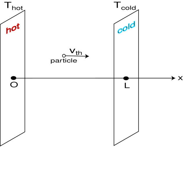
Figure 4: thermophoresis

This is another steady-state Cartesian one-dimensional problem with variation in the $x_{1}\equiv x$ direction only and $v_{1}\equiv v$ as the only non-zero velocity component.  Therefore, the $\overline{M}\left(D,\eta\right)$-formulation (15) linearized about the constant state,

$$\left(\overline{m},P,v,T\right)=\left(m_{\ast},P_{\ast},0,T_{\ast}\right),$$ (228)

where $T_{\ast}$ is the average temperature,

$$T_{\ast}=\frac{T_{\text{hot}}+T_{\text{cold}}}{2},$$ (229)

becomes

$$0 =\frac{dv}{dx}$$

$$0 =\frac{d^{2}P}{dx^{2}}$$ (230)

$$0 =-\frac{dP}{dx}+\eta_{\ast}\frac{d^{2}v}{dx^{2}}$$

$$0 =\frac{d^{2}T}{dx^{2}}.$$

Assuming the temperature of the fluid at the plates equals that of the plates, gives rise to the boundary conditions,

$$\left.T\right|_{x=0}=T_{\text{hot}}\text{ and }\left.T\right|_{x=L}=T_{\text{cold}},$$ (231)

and using these with equation (230 d) yields the linear temperature profile,

$$T\left(x\right)=T_{\text{hot}}-\left(\frac{T_{\text{hot}}-T_{\text{cold}}}{L}\right)x.$$ (232)

Furthermore, equations (230 a and c) imply that $v$ and $P$ are both constants.  Therefore,

$$P=P_{\ast},$$ (233)

and since the plates are impermeable, we may find $v$ by enforcing the no mass flux condition,

$$\left(j_{M}\right)_{1}=0,$$ (234)

where employing (232) and (233) in the one-dimensional version of (17), we have

$$\left(j_{M}\right)_{1}=-\left(m\alpha_{P}D\right)_{\ast}\left(\frac{T_{\text{hot}}-T_{\text{cold}}}{L}\right)+m_{\ast}v.$$ (235)

The constant velocity is then

$$v=\left(\alpha_{P}D\right)_{\ast}\left(\frac{T_{\text{hot}}-T_{\text{cold}}}{L}\right).$$ (236)

Therefore, my theory predicts a constant velocity in the $+x$ (colder) direction that is proportional to the fluid’s diffusion coefficient and thermal expansion coefficient and the size of the temperature gradient imposed between the plates.  If an insulated macroscopic particle were present in such a velocity field with a no-slip condition applied at its surface and no other forces acting on it, then the particle would simply be carried along at the fluid’s velocity, i.e. the particle’s thermophoretic velocity $v_{\text{th}}$ would equal the fluid’s continuum velocity $v$ computed above.

In contrast, when the non-convective mass flux is assumed to be zero, as in the case of the NSF formulation, the no mass flow condition (234) implies

$$v=0.$$ (237)

Consequently, thermophoretic motion does not arise in the same sense that it does for the $\overline{M}\left(D,\eta\right)$-formulation.  To account for thermophoresis with the NSF equations, one then finds it necessary to employ a thermal slip boundary condition at the particle’s surface at which there is assumed to be a non-zero tangential velocity proportional to the temperature gradient and in the down-gradient direction.  Under this assumption, various researchers have been led, theoretically and experimentally, to the following expression for the thermophoretic velocity in the case of an insulated particle in a gas:

$$\underline{v}_{\text{th}}=C_{\text{th}}\frac{\eta}{mT}\nabla T,$$ (238)

where $C_{\text{th}}$ is the thermal slip coefficient, dimensionless and theoretically believed to lie in the interval, $0.75\leq C_{\text{th}}\leq 1.5$, with $C_{\text{th}}\approx 1.17$ being a widely accepted theoretical estimate for gases.  For the problem considered here, (238) becomes

$$v_{\text{th}}=C_{\text{th}}\left(\frac{\eta}{mT}\right)_{\ast}\left(\frac{T_{\text{hot}}-T_{\text{cold}}}{L}\right).$$ (239)

Employing (I.72), which implies

$$\left(mD\right)_{\ast}=\left(C\eta\right)_{\ast},$$ (240)

and assuming an ideal gas for which the thermal expansion coefficient is given by (301), the thermophoretic velocity predicted by my theory in equation (236) may be expressed as

$$v_{\text{th}}=\left(C\frac{\eta}{mT}\right)_{\ast}\left(\frac{T_{\text{hot}}-T_{\text{cold}}}{L}\right).$$ (241)

Therefore, by identifying $C_{\ast}$ with $C_{\text{th}}$, one finds this to be the same as the thermal slip formula (239).  Also, recall that in §5, the value $C=7/6\approx 1.17$ was obtained for a classical monatomic ideal gas.

As discussed in Brenner [5], there is no real theory for thermal slip in a liquid.  Therefore, researchers, e.g. McNab and Meisen [22], typically apply the gas formulas to liquids, even though they admit that there is no theoretical justification for doing so.  For the idealized problem considered here, McNab and Meisen’s data corresponds to a thermal slip coefficient for water and $n$-hexane near room temperature of $C_{\text{th}}\approx 0.13$, an order of magnitude smaller than that of a gas.  Again using (240), but no longer assuming the ideal gas relationship (301), my theory’s thermophoretic velocity (236) becomes

$$v_{\text{th}}=-\left(C\frac{\eta\alpha_{P}}{m}\right)_{\ast}\left(\frac{T_{\text{hot}}-T_{\text{cold}}}{L}\right),$$ (242)

which when compared with the thermal slip formula (239), yields the relationship,

$$C_{\text{th}}=\left(CT\alpha_{P}\right)_{\ast}.$$ (243)

For water at $T_{\ast}=293$ K, we take $C_{\ast}=2.1$ (see appendix C) and $\left(\alpha_{P}\right)_{\ast}=2.05\times 10^{-4}$ K^-1 (from the CRC Handbook of Chemistry and Physics [9]), giving a slip coefficient value of $C_{\text{th}}=0.13$, which is the same as the experimental value mentioned above.

It is interesting to note that there is, in general, no positive definite restriction on the thermal expansion coefficient $\alpha_{P}$.  There exist equilibrium thermodynamic states in water and liquid helium, for example, in which $\alpha_{P}$ may vanish or become negative.  In view of equation (243), this means that such states could give rise to the occurrence of no thermophoresis or reverse thermophoresis.

12 Shock Waves

The problem examined below strains the limits of what one should expect from the NSF and $\overline{M}\left(D,\eta\right)$ formulations in two ways: (1) it is not near-equilibrium, which is counter to the assumption made in §4 and appendix B of part I used to justify linear constitutive laws and (2) it is a $K\!n\sim O\left(1\right)$ problem and, therefore, not in the hydrodynamic regime.  Nonetheless, the NSF equations are commonly employed as a qualitative tool for investigating the internal structure of shock waves, and so it is of interest to see how predictions from the $\overline{M}\left(D,\eta\right)$-formulation compare with these.

Let us consider a Cartesian one-dimensional steady-state shock wave like the one described in Zel’dovich and Raizer [36, pp. 469-482] and depicted schematically in figure 5 in a fixed reference frame.  Again, we assume variation is in the $x_{1}\equiv x$ direction only, $v_{1}\equiv v$ is the only non-zero component of the velocity, and there are no body forces.  The subscript ”$i$” is used to indicate undisturbed initial values ahead of the shock, and the subscript ”$f$” is used for final values after the shock moves through.  The initial and final fluid velocities are taken to be

$$v_{i}=0\text{ and }v_{f}=-v_{p},$$ (244)

where $v_{p}$ is the constant speed of the piston generating the shock wave.  For convenience, one transforms the problem into a coordinate system moving with the shock wave front as illustrated in figure 6, where primes denote variables in the moving coordinate system and $v_{s}$ represents the constant speed of the shock front.

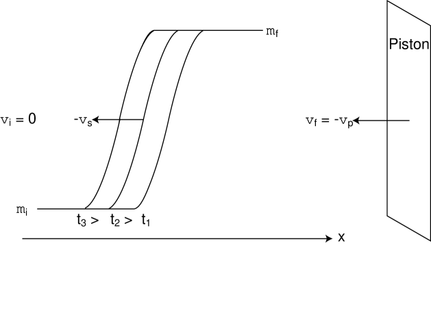
Figure 5: shock wave in a fixed coordinate system

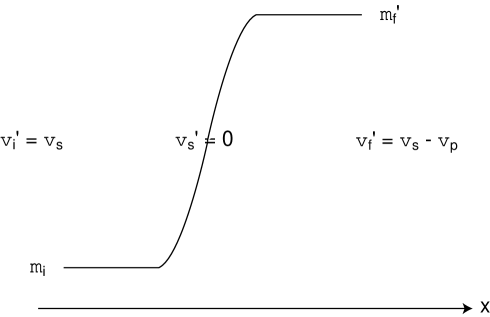
Figure 6: shock wave in a coordinate system moving with the front

Expressing the non-linear balance laws (1 a-c) and (7)–with constitutive equations (4), no body forces, and (I.18), (I.13), and $w=0$–in the one-dimensional moving coordinate system, making the steady-state assumption that the time derivatives vanish, using (291) and (292) to cast the system in terms of the variables, $\overline{m}^{\prime}$, $m^{\prime}$, $v^{\prime}$, and $T^{\prime}$, and employing the equilibrium thermodynamic relationships (300)-(302), (308), and (309) for a classical monatomic ideal gas, yields the following system of ordinary differential equations:

$$\frac{d}{dx^{\prime}}\left(\overline{m}^{\prime}v^{\prime}\right) =0$$ (245)

$$\frac{d}{dx^{\prime}}\left(-D^{\prime}\frac{dm^{\prime}}{dx^{\prime}}+m^{\prime}v^{\prime}\right) =0$$ (246)

$$\frac{d}{dx^{\prime}}\left(\frac{RT^{\prime}m^{\prime}}{A}-\overline{m}^{\prime}D^{\prime}\frac{dv_{x}^{\prime}}{dx^{\prime}}+\overline{m}^{\prime}v^{\prime 2}\right) =0$$ (247)

$$\frac{d}{dx^{\prime}}\left[\begin{array}[c]{c}-\frac{3R}{2A}D^{\prime}\frac{d\left(m^{\prime}T^{\prime}\right)}{dx^{\prime}}-\overline{m}^{\prime}D^{\prime}\frac{dv^{\prime}}{dx^{\prime}}v^{\prime}+\\ \left(\frac{5RT^{\prime}m^{\prime}}{2A\overline{m}^{\prime}}+\frac{1}{2}v^{\prime 2}\right)\overline{m}^{\prime}v^{\prime}\end{array}\right] =0.$$ (250)

For boundary conditions, let us assume that

$$\lim_{x^{\prime}\rightarrow-\infty}\overline{m}^{\prime}=m_{i}\text{, }\lim_{x^{\prime}\rightarrow-\infty}m^{\prime}=m_{i}\text{, }\lim_{x^{\prime}\rightarrow-\infty}v^{\prime}=v_{s}\text{, }\lim_{x^{\prime}\rightarrow-\infty}T^{\prime}=T_{i}$$ (251)

and

$$\lim_{x^{\prime}\rightarrow\infty}\overline{m}^{\prime}=\overline{m}_{f}\text{, }\lim_{x^{\prime}\rightarrow\infty}m^{\prime}=m_{f}\text{, }\lim_{x^{\prime}\rightarrow\infty}v^{\prime}=v_{s}-v_{p}\text{, }\lim_{x^{\prime}\rightarrow\infty}T^{\prime}=T_{f}$$ (252)

and that all gradients, $d\phi^{\prime}/dx^{\prime}$, vanish ahead of and behind the shock wave front, i.e.

$$\lim_{x^{\prime}\rightarrow-\infty}\frac{d\phi^{\prime}}{dx^{\prime}}=\lim_{x^{\prime}\rightarrow\infty}\frac{d\phi^{\prime}}{dx^{\prime}}=0,$$ (253)

where $\phi^{\prime}$ may represent any of the variables, $\overline{m}^{\prime}$, $m^{\prime}$, $v^{\prime}$, or $T^{\prime}$.  Then, by integrating (245)-(250) from $-\infty$ to $x^{\prime}$, one finds

$$\overline{m}^{\prime}v^{\prime} =m_{i}v_{s}$$ (254)

$$D^{\prime}\frac{dm^{\prime}}{dx^{\prime}} =\left(\frac{m^{\prime}}{\overline{m}^{\prime}}-1\right)m_{i}v_{s}$$ (255)

$$\overline{m}^{\prime}D^{\prime}\frac{dv^{\prime}}{dx^{\prime}} =\frac{R}{A}\left(T^{\prime}m^{\prime}-T_{i}m_{i}\right)+\left(v^{\prime}-v_{s}\right)m_{i}v_{s}$$ (256)

$$\frac{3R}{2A}D^{\prime}\frac{d\left(m^{\prime}T^{\prime}\right)}{dx^{\prime}} =\left[\begin{array}[c]{c}-D^{\prime}\frac{dv^{\prime}}{dx^{\prime}}+\\ \left(\frac{5RT^{\prime}m^{\prime}}{2A\overline{m}^{\prime}}-\frac{5RT_{i}}{2A}\right)+\\ \frac{1}{2}\left(v^{\prime 2}-v_{s}^{2}\right)\end{array}\right]m_{i}v_{s},$$ (260)

where (254) has been employed in writing equations (255)-(260), and by taking the limit of the above equations as $x^{\prime}\rightarrow\infty$, one arrives at the relations

$$\overline{m}_{f}=\frac{m_{i}v_{s}}{\left(v_{s}-v_{p}\right)}$$ (261)

$$m_{f}=\overline{m}_{f}$$ (262)

$$T_{f}=\frac{\left(v_{s}-v_{p}\right)}{v_{s}}\left(T_{i}+\frac{A}{R}v_{s}v_{p}\right)$$ (263)

$$v_{s}^{2}-\frac{4}{3}v_{s}v_{p}-\frac{5RT_{i}}{3A}=0,$$ (264)

where (261) and (262) have been used to write (263), and (262) and (263) have been used to obtain (264).  One solves (264) for the positive root to find the following expression for the shock speed:

$$v_{s}=\frac{2}{3}\left(v_{p}+\sqrt{v_{p}^{2}+\frac{15RT_{i}}{4A}}\right).$$ (265)

Therefore, if the initial mass density and temperature, $m_{i}$ and $T_{i}$, and the piston speed, $v_{p}$, are known, then all of the relevant final values, $\overline{m}_{f}$, $m_{f}$, $T_{f}$, and $v_{f}^{\prime}=v_{s}-v_{p}$, may be computed via (265) and (261)-(263) for a classical monatomic ideal gas.  Note that these are identical to the shock speed and final values found with the NSF equations.

Using the same assumptions and carrying out the foregoing procedure for the NSF formulation, yields the following system:

$$m^{\prime}v^{\prime} =m_{i}v_{s}$$ (266)

$$\frac{4}{3}\eta^{\prime}\frac{dv^{\prime}}{dx^{\prime}} =\frac{R}{A}\left(T^{\prime}m^{\prime}-T_{i}m_{i}\right)+\left(v^{\prime}-v_{s}\right)m_{i}v_{s}$$ (267)

$$\frac{15R}{4A}\eta^{\prime}\frac{dT^{\prime}}{dx^{\prime}} =\left[\begin{array}[c]{c}-\frac{4\eta^{\prime}}{3m^{\prime}}\frac{dv^{\prime}}{dx^{\prime}}+\\ \left(\frac{5RT^{\prime}}{2A}-\frac{5RT_{i}}{2A}\right)+\\ \frac{1}{2}\left(v^{\prime 2}-v_{s}^{2}\right)\end{array}\right]m_{i}v_{s}$$ (271)

with boundary conditions (251 b-d), (252 b-d), and (253).  In the above, the classical monatomic ideal gas assumptions (78) and (306) have been used.

For this non-linear problem, the longitudinal diffusion coefficient, $D^{\prime}$, and the shear viscosity, $\eta^{\prime}$, may depend on state variables, e.g. it is common to express the viscosity with a temperature power law of the form (310):

$$\eta\left(T\right)=\eta_{r}\left(\frac{T}{T_{r}}\right)^{\beta},$$

where $T_{r}$ is some reference temperature and $\eta_{r}$ is the viscosity measured at $T_{r}$ (see appendix C).  Also, in appendix C, it is shown that in a classical monatomic ideal gas one might reasonably take (313):

$$\left(\overline{m}D\right)\left(T\right)=\frac{7}{6}\eta_{r}\left(\frac{T}{T_{r}}\right)^{\beta}$$

Figures 7 and 8 contain plots of numerical solutions to dimensionless versions of (254)-(260) and (266)-(271) with their appropriate boundary conditions and power laws (310) and (313) describing the transport coefficients.  The numerical method employed is iterative Newton’s method with centered differences approximating the spatial derivatives.  The dimensionless variables used are

$$x^{\prime\prime}=\frac{x^{\prime}}{\lambda_{i}}\text{, }v^{\prime\prime}=\frac{v^{\prime}}{c_{i}}\text{, }\overline{m}^{\prime\prime}=\frac{\overline{m}^{\prime}}{m_{i}}\text{, }m^{\prime\prime}=\frac{m^{\prime}}{m_{i}}\text{, and }T^{\prime\prime}=\frac{T^{\prime}}{T_{i}},$$ (272)

where $\lambda_{i}$ and $c_{i}$ are the mean free path length and adiabatic sound speed in the initial state, and the Mach number is computed as

$$M\!a=\frac{v_{s}}{c_{i}}.$$ (273)

Each of the figures corresponds to $M\!a=2.05$ with parameters chosen to be those of Alsmeyer [1] for his shock wave experiments in argon gas: the undisturbed initial values,

$$T_{i} =300\text{ K}$$

$$m_{i} =1.07\times 10^{-4}\text{ kg/m}^{3}\text{ (for }P_{i}=6.67\text{ Pa)}$$

$$\lambda_{i} =1.10\times 10^{-3}\text{ m}$$

$$c_{i} =323\text{ m/s}$$

and the parameters appearing in (310),

$$T_{r}=300\text{ K, }\eta_{r}=2.31\times 10^{-5}\text{ kg/(m}\cdot\text{s), and }\beta=0.72.$$

The curves plotted in figures 7 and 8 are the normalized mass density, $m^{\prime\prime\prime}=\left(m^{\prime}-m_{i}\right)/\left(m_{f}-m_{i}\right)$ (in blue), the normalized fluid speed, $v^{\prime\prime\prime}=\left(v^{\prime}-v_{i}^{\prime}\right)/(v_{f}^{\prime}-v_{i}^{\prime})$ (in green), and the normalized temperature, $T^{\prime\prime\prime}=\left(T^{\prime}-T_{i}\right)/\left(T_{f}-T_{i}\right)$ (in red) versus the dimensionless position, $x^{\prime\prime}$.  Since the numerical solution sets are arbitrarily positioned on the $x^{\prime\prime}$-axis, the $x^{\prime\prime}=0$ point is chosen to be the center of the mass density profile (the point at which the highest slope of $m^{\prime\prime}$ occurs).  Figure 7 contains the normalized shock wave profiles predicted by the $\overline{M}\left(D,\eta\right)$-formulation and figure 8 contains those predicted by the NSF formulation.  Comparing the curves in these two figures, one observes that the mass density, temperature, and fluid velocity profiles are much closer together in my theory than for the NSF formulation.  This difference is perhaps most obvious in the leading edge of the shock wave (the $x^{\prime\prime}<0$ side) where my theory predicts these three profiles to be very near one another, whereas NSF predicts a pronounced displacement between the three with temperature leading, velocity behind it, and mass density in the back.  I am unfamiliar with any direct physical arguments or experimental evidence that would explain why these profiles should be displaced in such a manner.  Therefore, it would be very interesting to obtain measurements revealing the structure and position of these quantities.  Experiments, such as Alsmeyer’s, which have been conducted to probe the internal structure of shock waves in a gas, measure only the mass density profile.

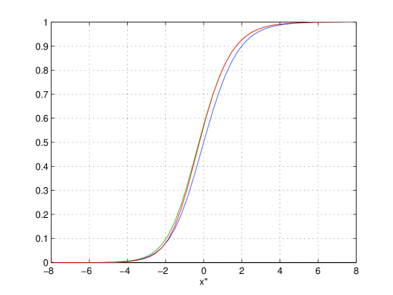
Figure 7: numerically computed shock wave profiles: $\overline{M}\left(D,\eta\right)$ - formulation

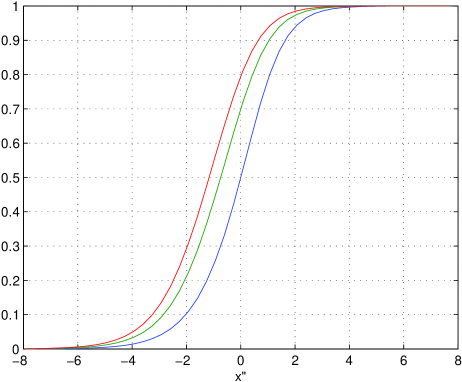
Figure 8: numerically computed shock wave profiles: NSF formulation

13 Future Work

To advance the study of single-component fluids with the $\overline{M}\left(D,\eta\right)$-formulation, there are two major tasks that lie ahead: (1) to further investigate non-linear phenomena and (2) to reconcile the $\overline{M}\left(D,\eta\right)$-description with macroscopic behavior observed outside of the hydrodynamic regime, i.e. in the transition and rarefied gas regimes.  First, however, there remain a few important details to address regarding the linearized equations in the hydrodynamic regime.  I treat these topics, mentioned below, in future papers.

• I recast the linearized $\overline{M}$-formulation (which includes both the linearized $\overline{M}\left(D,\eta\right)$ and NSF descriptions) in the following way.  Using Legendre transformations, I reexpress the equations of motion in terms of variables, $\overline{m}$, $P$, $\underline{p}$, $\sigma$. Afterwards, I normalize these variables in a way that facilitates the study of hydrodynamical fluctuations, as treated in [27].

• For the recast linearized $\overline{M}$-formulation, I compute Green’s functions on one and three-dimensional infinite spatial domains.  These are then used to give a complete mathematical description of (1) the equilibration of initial disturbances in an infinite fluid and (2) sound waves emanating from a vibrating source into an infinite fluid.

• The method of images is used to produce Green’s functions for the linearized $\overline{M}$-formulation on a one-dimensional semi-infinite spatial domain with boundary conditions that prescribe

  $$\nabla P\cdot\underline{n}\text{, }\nabla\sigma\cdot\underline{n}\text{, and }\underline{p}\cdot\underline{n}$$ (274)

  where $\underline{n}$ represents the outward unit normal to the boundary.  These Green’s functions are employed to gain a complete mathematical description of one-dimensional disturbances in a fluid interacting with an impermeable, infinite impedance wall.

• Green’s functions are found for the linearized $\overline{M}$-formulation on a one-dimensional finite spatial domain with boundary conditions of type (274) in order to study sound resonators of infinite impedance.

• The variables in the one-dimensional $\overline{M}\left(D,\eta\right)$-formulation are further recast in order to isolate the right-going and left-going parts of the solution.  Green’s functions are found for this recast system on infinite, semi-infinite, and finite spatial domains to use in the study of fluid disturbances interacting with non-infinite impedance walls.

• A detailed examination of stationary-Gaussian-Markov processes is carried out in order to give a complete stochastical description of linearized hydrodynamics with the $\overline{M}$-formulation.  I divide this treatment into three parts: I. general theory, II. Brownian oscillators and, III. hydrodynamical fluctuations.

Of course, there are eventually more complicated systems to be considered, such as solids, multicomponent media, and electrically charged media.  I wish to treat all of these topics analogously to the way I have treated single-component fluids.  This will inevitably lead to descriptions that are different from the ones currently used.  As with the $\overline{M}\left(D,\eta\right)$-formulation for single-component fluids, I will ensure there is full agreement with the standard models when physical, but there may also arise disagreement in predictions–some testable by experiment and others leading to new interpretations of phenomena.

Acknowledgement

Well beyond the typical debt of gratitude a daughter owes her father, do I owe mine, Marvin Morris.  He has done literature searches, procured references, and created the figures and graphs appearing in this paper, but most importantly he has been my adviser in helping me map out a path through these studies.

Appendix A Tensors

In this paper, I use the following identity:

$$\nabla\cdot\left[\left(\nabla\underline{w}\right)^{sy,dev}\right]=\frac{1}{2}\nabla^{2}\underline{w}+\frac{1}{6}\nabla\left(\nabla\cdot\underline{w}\right),$$ (275)

and cylindrical coordinate formulas:

$$\left(\nabla\alpha\right)_{r} =\frac{\partial\alpha}{\partial r}$$ (276)

$$\left(\nabla\alpha\right)_{\theta} =\frac{1}{r}\frac{\partial\alpha}{\partial\theta}$$ (277)

$$\left(\nabla\alpha\right)_{z} =\frac{\partial\alpha}{\partial z}$$ (278)

$$\nabla^{2}\alpha=\frac{1}{r}\frac{\partial}{\partial r}\left(r\frac{\partial\alpha}{\partial r}\right)+\frac{1}{r^{2}}\frac{\partial^{2}\alpha}{\partial\theta^{2}}+\frac{\partial^{2}\alpha}{\partial z^{2}}$$ (279)

$$\nabla\cdot\underline{w}=\frac{1}{r}\frac{\partial}{\partial r}\left(rw_{r}\right)+\frac{1}{r}\frac{\partial w_{\theta}}{\partial\theta}+\frac{\partial w_{z}}{\partial z}$$ (280)

$$\left(\nabla^{2}\underline{w}\right)_{r} =\frac{\partial}{\partial r}\left[\frac{1}{r}\frac{\partial}{\partial r}\left(rw_{r}\right)\right]+\frac{1}{r^{2}}\frac{\partial^{2}w_{r}}{\partial\theta^{2}}+\frac{\partial^{2}w_{r}}{\partial z^{2}}-\frac{2}{r^{2}}\frac{\partial w_{\theta}}{\partial\theta}$$ (281)

$$\left(\nabla^{2}\underline{w}\right)_{\theta} =\frac{\partial}{\partial r}\left[\frac{1}{r}\frac{\partial}{\partial r}\left(rw_{\theta}\right)\right]+\frac{1}{r^{2}}\frac{\partial^{2}w_{\theta}}{\partial\theta^{2}}+\frac{\partial^{2}w_{\theta}}{\partial z^{2}}+\frac{2}{r^{2}}\frac{\partial w_{r}}{\partial\theta}$$ (282)

$$\left(\nabla^{2}\underline{w}\right)_{z} =\frac{1}{r}\frac{\partial}{\partial r}\left(r\frac{\partial w_{z}}{\partial r}\right)+\frac{1}{r^{2}}\frac{\partial^{2}w_{z}}{\partial\theta^{2}}+\frac{\partial^{2}w_{z}}{\partial z^{2}}.$$ (283)

Appendix B Equilibrium Thermodynamic Relationships

In addition to the thermodynamic parameters mentioned in §2 and appendix C of part I, let us introduce the specific entropy $\sigma$, isobaric specific heat per mass $c_{P}$, isobaric to isochoric specific heat ratio $\gamma=c_{P}/c_{V}$, adiabatic sound speed $c$, the particle number density,

$$n_{p}=\frac{N_{A}}{A}m,$$ (284)

where $N_{A}$ and $A$ respectively denote Avogadro’s number and the atomic weight, and the particle number $N_{p}=n_{p}V$.  All of these quantities are defined in Callen [6].

For thermodynamically stable classical systems, in addition to (I.156) and (I.157), the following inequalities hold:

$$\sigma,c_{P},c>0,$$ (285)

and

$$\gamma\geq 1.$$ (286)

Note the following general equilibrium thermodynamic relationships:

$$h_{M}=\frac{u+P}{m}$$ (287)

$$\kappa_{T}=\frac{\gamma}{mc^{2}}$$ (288)

$$\frac{T\alpha_{P}}{m\kappa_{T}c_{V}}=\frac{\left(\gamma-1\right)}{\alpha_{P}}$$ (289)

$$\gamma-1=\frac{T\alpha_{P}^{2}c^{2}}{c_{P}}$$ (290)

$$du =mc_{V}dT+\left(h_{M}-\frac{T\alpha_{P}}{m\kappa_{T}}\right)dm$$ (291)

$$dP =\frac{\alpha_{P}}{\kappa_{T}}dT+\frac{1}{m\kappa_{T}}dm$$ (292)

$$du =m\left(c_{P}-h_{M}\alpha_{P}\right)dT+\left(\frac{h_{M}\gamma}{c^{2}}-T\alpha_{P}\right)dP$$ (293)

$$dm =-m\alpha_{P}dT+\frac{\gamma}{c^{2}}dP$$ (294)

and

$$d\sigma=\frac{c_{P}}{T}dT-\frac{\alpha_{P}}{m}dP$$ (295)

where equations (291)-(295) may be derived by using Legendre transformations, as detailed in Callen [6, §5.3].

The equilibrium thermodynamic fluctuation formulas below may be found with the methods in Callen [6, Ch. 15].  The following are second moments that apply to a thermodynamic system of fixed volume $V$ in contact with a heat/particle reservoir:

$$\left\langle\delta\!m^{2}\right\rangle_{V} =\frac{k_{B}m^{2}T\kappa_{T}}{V}$$ (296)

$$\left\langle\delta\!u^{2}\right\rangle_{V} =\frac{k_{B}mT}{V}\left[Tc_{V}+m\kappa_{T}\left(h_{M}-\frac{T\alpha_{P}}{m\kappa_{T}}\right)^{2}\right]$$ (297)

$$\left\langle\delta\!m\delta\!u\right\rangle_{V} =\frac{k_{B}m^{2}T\kappa_{T}}{V}\left(h_{M}-\frac{T\alpha_{P}}{m\kappa_{T}}\right)$$ (298)

$$\left\langle\delta\!N_{p}^{2}\right\rangle_{V} =k_{B}n_{p}^{2}T\kappa_{T}V$$ (299)

where $k_{B}$ denotes the Boltzmann constant.

Note the following classical ideal gas formulas:

$$P=\frac{RTm}{A}$$ (300)

$$\alpha_{P}=\frac{1}{T}$$ (301)

$$\kappa_{T}=\frac{A}{RTm}$$ (302)

$$c_{P}=\frac{R\gamma}{A\left(\gamma-1\right)}$$ (303)

$$c=\sqrt{\frac{\gamma RT}{A}}$$ (304)

$$d\sigma=\frac{R\gamma}{A\left(\gamma-1\right)T}dT-\frac{R}{AP}dP\text{ (when }c_{V}\text{\ is constant)}$$ (305)

and classical monatomic ideal gas formulas:

$$\gamma=\frac{5}{3}$$ (306)

$$c=\sqrt{\frac{5RT}{3A}}$$ (307)

$$u=\frac{3RTm}{2A}$$ (308)

$$c_{V}=\frac{3R}{2A}$$ (309)

where $R$ is the universal gas constant and $A$ represents the atomic weight of the gas.

Appendix C Values for $D$

Here, measured sound propagation data is used together with formulas from §5 to compute the longitudinal diffusion coefficient, $D$, of the $\overline{M}\left(D,\eta\right)$-formulation for various types of fluids.  The temperature and pressure dependence of this parameter is explored where data is available.  In the future, I hope to obtain more (and more reliable) data with which to refine these estimates and to include values for additional fluids.

Values at Normal Temperature and Pressure

Table 1 provides values of the $\overline{M}\left(D,\eta\right)$-formulation diffusion coefficient, $D_{\text{eq}}$, the self-diffusion coefficient, $\left(D_{\text{self}}\right)_{\text{eq}}$, (where available), and the dimensionless parameter $C_{\text{eq}}$ defined via equation (80), for several gases and liquids at $T_{\text{eq}}=300$ K (unless indicated otherwise) and $P_{\text{eq}}=1.013\times 10^{5}$ Pa.

Table 1: diffusion parameters for various fluids at normal temperature and pressure

fluid	$\begin{array}[c]{c}D_{\text{eq}}\\ (\text{m}^{2}/\text{s})\end{array}$	$\begin{array}[c]{c}\left(D_{\text{self}}\right)_{\text{eq}}\\ (\text{m}^{2}/\text{s})\end{array}$	$C_{\text{eq}}$	$\begin{array}[c]{c}\left(\overline{m}D\right)_{\text{eq}}\\ (\text{kg}/(\text{m}\cdot\text{s}))\end{array}$
gases
helium	$1.44\times 10^{-4}$	$1.82\times 10^{-4}$	$1.17$	$2.34\times 10^{-5}$
neon	$4.57\times 10^{-5}$	$5.25\times 10^{-5}$	$1.17$	$3.75\times 10^{-5}$
argon	$1.64\times 10^{-5}$	$1.84\times 10^{-5}$	$1.17$	$2.66\times 10^{-5}$
krypton	$8.77\times 10^{-6}$	$9.84\times 10^{-6}$	$1.17$	$2.99\times 10^{-5}$
xenon	$5.07\times 10^{-6}$	$5.76\times 10^{-6}$	$1.17$	$2.70\times 10^{-5}$
nitrogen	$2.01\times 10^{-5}$	$2.12\times 10^{-5}$ †	$1.28$	$2.29\times 10^{-5}$
oxygen	$1.79\times 10^{-5}$	$2.32\times 10^{-5}$ †	$1.12$	$2.33\times 10^{-5}$
carbon dioxide	$1.08\times 10^{-5}$	$1.13\times 10^{-5}$ †	$1.29$	$1.93\times 10^{-5}$
methane	$2.59\times 10^{-5}$	$2.40\times 10^{-5}$ †	$1.51$	$1.69\times 10^{-5}$
air	$1.96\times 10^{-5}$		$1.26$	$2.17\times 10^{-5}$
liquids
water	$1.6\times 10^{-6}$ ‡	$2.60\times 10^{-9}$ ‡	$2.0$ ‡	$1.6\times 10^{-3}$ ‡
mercury	$4.5\times 10^{-7}$ ‡	$5.7\times 10^{-9}$ ‡	$4.1$ ‡	$6.1\times 10^{-3}$ ‡
glycerol	$5.4\times 10^{-4}$ †	$1.9\times 10^{-12}$ †	$0.78$ †	$6.8\times 10^{-1}$ †
benzene	$4.8\times 10^{-5}$ †	$2.2\times 10^{-9}$ †	$70$ †	$4.22\times 10^{-2}$ †
ethyl alcohol	$1.9\times 10^{-6}$ †	$1.4\times 10^{-9}$ †	$1.4$ †	$1.5\times 10^{-3}$ †
castor oil	$4.4\times 10^{-4}$ †		$0.43$ †	$4.2\times 10^{-1}$ †
$\begin{array}[c]{c}{\dagger}\text{ at }T_{\text{eq}}=298\text{ K}\\ {\ddagger}\text{ at }T_{\text{eq}}=303\text{ K}\end{array}$

For the noble gases, helium, neon, argon, krypton, and xenon, $C_{\text{eq}}$ is given by (81) and the diffusion coefficient is computed via (79) with shear viscosities from Kestin et al. [18] and mass densities determined by the classical ideal gas relationship (300), which is appropriate for each of the table 1 gases in the normal temperature and pressure regime.  For the diatomic gases, nitrogen and oxygen, and the polyatomic gases, carbon dioxide and methane, $D_{\text{eq}}$ and $C_{\text{eq}}$ are computed by equations (77) and (80), respectively, using data presented in Marques [21], viscosity data from Cole and Wakeham [8] and Trengrove and Wakeham [34], and mass densities computed via relation (300).  For air and the liquids, $D_{\text{eq}}$ is computed via equation (71) and $C_{\text{eq}}$ by relation (80).  The sound propagation quantities, $\alpha/f^{2}$ and $c_{\text{eq}}$, are calculated for air using [42] with $f=11$ MHz and $0\%$ humidity, given for mercury in Hunter et al. [17], and tabulated for the rest of the liquids in [45].  The viscosities and mass densities are taken from [44] for air, [46] for water, [17] for mercury, [43] for glycerol, [40] and [41] for benzene, [38] for ethyl alcohol, and [40] and [37] for castor oil.  The self-diffusion coefficients are taken from Kestin et al. [18] for the noble gases, from Winn [35] for the diatomic and polyatomic gases, from Holz et al. [16] for water, from Nachtrieb and Petit [29] for mercury, from Tomlinson [32] for glycerol, from Kim and Lee [19] for benzene, and from Meckl and Zeidler [23] for ethyl alcohol.

From the values presented in table 1, one makes the following observations.

• In each of the gases, the diffusion and self-diffusion coefficients are observed to be the same order of magnitude.  However in liquids, the self-diffusion coefficients are several orders of magnitude smaller than the $D_{\text{eq}}$ values.  This indicates that although in gases the diffusion coefficient may be roughly approximated by self-diffusion, the same may not be said of liquids.

• The diffusion parameters of the noble gases are seen to decrease with increasing mass density.

• The value for $D_{\text{eq}}$ in air is approximately a weighted average of the $D_{\text{eq}}$ values for nitrogen and oxygen based on their fractional compositions in air ($\approx 0.8$ nitrogen and $\approx 0.2$ oxygen).

• With the exception of very light gases like helium and very heavy gases like krypton and xenon, diffusion coefficients for gases at normal temperature and pressure are typically on the order of $10^{-5}$ m${}^{2}/$s.

• The $D_{\text{eq}}$ values of water and ethyl alcohol–which fall into the category of medium viscosity, medium density liquids–are similar and on the order of $10^{-6}$ m${}^{2}/$s, an order of magnitude smaller than that of a typical gas.  The high viscosity, medium density liquids, glycerol and castor oil, possess similar $D_{\text{eq}}$ values on the higher order of $10^{-4}$ m${}^{2}/$s.  Mercury’s viscosity is medium range like water and ethyl alcohol, but its much higher mass density results in a smaller $D_{\text{eq}}$ on the order of $10^{-7}$ m${}^{2}/$s.

• At normal temperature and pressure, all of the gases have $\left(\overline{m}D\right)_{\text{eq}}$ on the order of $10^{-5}$ kg/(m$\cdot$s) with this quantity not varying much from gas to gas; and all of the liquids have much higher values for $\left(\overline{m}D\right)_{\text{eq}}$ with orders varying from $10^{-3}$ to $10^{-1}$ kg/(m$\cdot$s) and the highest values belonging to the most viscous fluids, glycerol and castor oil.

Dependence on State Parameters

Gases

In general, it is observed from sound attenuation data for gases in the hydrodynamic regime that the product, $\left(\overline{m}D\right)_{\text{eq}}=m_{\text{eq}}D_{\text{eq}}$, may vary with temperature but has negligible pressure dependence at a fixed temperature.  Using this observation, together with relationship (I.72) and the fact that the shear viscosity $\eta$ also has negligible pressure dependence, leads us to conclude that, although $C$ is possibly a function of $T$, it does not tend to vary much with $P$ for gases.  Typically, $\eta$ may be expressed as a temperature power law of the form,

$$\eta=\eta_{r}\left(\frac{T}{T_{r}}\right)^{\beta},$$ (310)

where $T_{r}$ is some reference temperature and $\eta_{r}$ is the viscosity measured at $T_{r}$.  Using this in equation (I.7.7), one finds

$$\left(\overline{m}D\right)\left(T\right)=\eta_{r}C\left(T\right)\left(\frac{T}{T_{r}}\right)^{\beta}.$$ (311)

Equations (77) and (80) together imply

$$C_{\text{eq}}=\frac{1}{2}\left\{\frac{\zeta_{NS}}{\eta}+\left[\frac{4}{3}+\left(1-\frac{1}{\gamma}\right)E\!u\right]\right\}_{\text{eq}}.$$ (312)

For noble gases, such as argon, one expects the values for $\left(\zeta_{NS}\right)_{\text{eq}}$, $\gamma_{\text{eq}}$, and $E\!u_{\text{eq}}$ given in (78) to hold over a broad temperature range.  Therefore, in the noble gases, we take $C=7/6$ to be constant and, substituting this into (311),

$$\left(\overline{m}D\right)\left(T\right)=\frac{7}{6}\eta_{r}\left(\frac{T}{T_{r}}\right)^{\beta}.$$ (313)

On the other hand, as observed in tables 2-4, for non-monatomic gases such as air, nitrogen, and methane, $C$ displays a tendency to increase with temperature.  In tables 2-4, the $D_{\text{eq}}$ values are computed by equation (71) with $\alpha/f^{2}$ calculated using [42] for air with $f=11$ MHz and $0\%$ humidity and taken from [30] for nitrogen and methane and with $c_{\text{eq}}$ computed from the classical ideal gas formula (304), where the $\gamma_{\text{eq}}$ values are taken from [44] for air and approximated to be constant over the studied temperature range for nitrogen and methane with respective values $1.4$ and $1.3$.  The $C_{\text{eq}}$ values appearing in tables 2-4 are computed via equation (80) with shear viscosities taken from [44] for air and from [30] for nitrogen and methane and mass densities taken from [44] for air and computed by ideal gas formula (300) for nitrogen and methane.

Table 2: diffusion coefficient for air at atmospheric pressure and various temperatures

$T_{\text{eq}}$ (K)	$D_{\text{eq}}$ (m${}^{2}/$s)	$C_{\text{eq}}$	$\left(\overline{m}D\right)_{\text{eq}}$ (kg/(m$\cdot$s))
$253$	$1.40\times 10^{-5}$	$1.22$	$1.96\times 10^{-5}$
$263$	$1.52\times 10^{-5}$	$1.23$	$2.04\times 10^{-5}$
$273$	$1.64\times 10^{-5}$	$1.24$	$2.11\times 10^{-5}$
$283$	$1.76\times 10^{-5}$	$1.25$	$2.19\times 10^{-5}$
$288.15$	$1.82\times 10^{-5}$	$1.25$	$2.23\times 10^{-5}$
$293$	$1.88\times 10^{-5}$	$1.26$	$2.27\times 10^{-5}$
$303$	$2.01\times 10^{-5}$	$1.27$	$2.35\times 10^{-5}$
$313$	$2.15\times 10^{-5}$	$1.27$	$2.42\times 10^{-5}$
$323$	$2.29\times 10^{-5}$	$1.28$	$2.50\times 10^{-5}$

Table 3: diffusion coefficient for nitrogen gas at 0.01 atm and various temperatures

$T_{\text{eq}}$ (K)	$D_{\text{eq}}$ (m${}^{2}/$s)	$C_{\text{eq}}$	$\left(\overline{m}D\right)_{\text{eq}}$ (kg/(m$\cdot$s))
$77.1$	$1.37\times 10^{-4}$	$1.11$	$6.09\times 10^{-6}$
$180$	$7.63\times 10^{-4}$	$1.22$	$1.42\times 10^{-5}$
$260$	$1.57\times 10^{-3}$	$1.29$	$2.06\times 10^{-5}$
$293$	$1.97\times 10^{-3}$	$1.31$	$2.32\times 10^{-5}$

Table 4: diffusion coefficient for methane gas at 0.01 atm and various temperatures

$T_{\text{eq}}$ (K)	$D_{\text{eq}}$ (m${}^{2}/$s)	$C_{\text{eq}}$	$\left(\overline{m}D\right)_{\text{eq}}$ (kg/(m$\cdot$s))
$77.1$	$1.58\times 10^{-4}$	$1.26$	$4.00\times 10^{-6}$
$180$	$8.84\times 10^{-4}$	$1.36$	$9.79\times 10^{-6}$
$260$	$1.92\times 10^{-3}$	$1.47$	$1.44\times 10^{-5}$
$293$	$2.49\times 10^{-3}$	$1.52$	$1.64\times 10^{-5}$

The following are least squares fits to the data appearing in tables 2-4:

$$\left(\overline{m}D\right)_{\text{eq}} =2.32\times 10^{-5}\left[\frac{T_{\text{eq}}\text{ }\left(\text{in K}\right)}{300}\right]^{1.00}\text{ kg/(m}\cdot\text{s) for air}$$ (314)

$$\left(\overline{m}D\right)_{\text{eq}} =2.38\times 10^{-5}\left[\frac{T_{\text{eq}}\text{ }\left(\text{in K}\right)}{300}\right]^{1.00}\text{ kg/(m}\cdot\text{s) for N}_{2}\text{(g)}$$ (315)

$$\left(\overline{m}D\right)_{\text{eq}} =1.68\times 10^{-5}\left[\frac{T_{\text{eq}}\text{ }\left(\text{in K}\right)}{300}\right]^{1.05}\text{ kg/(m}\cdot\text{s) for CH}_{4}\text{(g).}$$ (316)

Liquids

Using equations (71) and (80) with sound speed and attenuation data from [45] and mass density and shear viscosity data from [46], one obtains the estimates of $D_{\text{eq}}$ and $C_{\text{eq}}$ for water at atmospheric pressure ($P_{\text{eq}}=1.013\times 10^{5}$ Pa) and various temperatures $T_{\text{eq}}$ between the freezing and boiling point appearing in table 5.

Table 5: diffusion parameters for water at atmospheric pressure and various temperatures between the freezing and boiling point

$T_{\text{eq}}$ (K)	$D_{\text{eq}}$ (m2/s)	$\left(D_{\text{self}}\right)_{\text{eq}}$ (m2/s)	$C_{\text{eq}}$	$\left(\overline{m}D\right)_{\text{eq}}$ (kg/(m$\cdot$s))
$273$	$4.0\times 10^{-6}$	$1.10\times 10^{-9}$	$2.2$	$4.0\times 10^{-3}$
$283$	$2.8\times 10^{-6}$	$1.53\times 10^{-9}$	$2.1$	$2.8\times 10^{-3}$
$293$	$2.1\times 10^{-6}$	$2.02\times 10^{-9}$	$2.1$	$2.1\times 10^{-3}$
$303$	$1.6\times 10^{-6}$	$2.59\times 10^{-9}$	$2.0$	$1.6\times 10^{-3}$
$313$	$1.3\times 10^{-6}$	$3.24\times 10^{-9}$	$2.0$	$1.3\times 10^{-3}$
$323$	$1.1\times 10^{-6}$	$3.96\times 10^{-9}$	$2.0$	$1.1\times 10^{-3}$
$333$	$9.5\times 10^{-7}$	$4.75\times 10^{-9}$	$2.0$	$9.3\times 10^{-4}$
$343$	$8.3\times 10^{-7}$	$5.62\times 10^{-9}$	$2.0$	$8.1\times 10^{-4}$
$353$	$7.5\times 10^{-7}$	$6.56\times 10^{-9}$	$2.1$	$7.3\times 10^{-4}$
$363$	$6.9\times 10^{-7}$	$7.57\times 10^{-9}$	$2.1$	$6.7\times 10^{-4}$
$373$	$6.5\times 10^{-7}$	$8.67\times 10^{-9}$	$2.2$	$6.2\times 10^{-4}$

As one can see, the parameter $C_{\text{eq}}$ does not vary much over the entire temperature range, but $D_{\text{eq}}$ and $\left(\overline{m}D\right)_{\text{eq}}$ decrease with temperature.  Excellent least squares fits are made to the water data in table 5 with

$$D_{\text{eq}}=3.9853\times 10^{-7}\exp\left(\frac{3.5115\times 10^{12}}{T_{\text{eq}}^{5}}\right)\text{ m}^{2}\text{/s}$$ (317)

and

$$\left(\overline{m}D\right)_{\text{eq}}=3.8262\times 10^{-4}\exp\left(\frac{3.5899\times 10^{12}}{T_{\text{eq}}^{5}}\right)\text{ kg/(m}\cdot\text{s)}$$ (318)

where $T_{\text{eq}}$ is in Kelvin.  In the third column of table 5, measured self-diffusion coefficients from Holz et al. [16] are tabulated for water at atmospheric pressure.  Unlike our observation for gases, these self-diffusions are two to three orders of magnitude less than the corresponding $D_{\text{eq}}$ values.  Also, unlike $D_{\text{eq}}$, the self-diffusion increases with temperature.

In table 6, $D_{\text{eq}}$ and $C_{\text{eq}}$ are computed for water at two fixed temperatures, $273$ K and $303$ K, and various pressures roughly between $1$ and $2000$ atmospheres. The values are obtained using equations (71) and (80) together with data presented in Litovitz and Carnevale [20].

Table 6: diffusion coefficient for water at 273 K and 303 K and various pressures

$P_{\text{eq}}$ (Pa)	$D_{\text{eq}}$ (m2/s)	$C_{\text{eq}}$	$\left(\overline{m}D\right)_{\text{eq}}$ (kg/(m$\cdot$s))
$T_{\text{eq}}=273$ K
$9.81\times 10^{4}$	$4.03\times 10^{-6}$	$2.25$	$4.03\times 10^{-3}$
$4.90\times 10^{7}$	$3.96\times 10^{-6}$	$2.43$	$4.08\times 10^{-3}$
$9.81\times 10^{7}$	$3.85\times 10^{-6}$	$2.42$	$3.93\times 10^{-3}$
$1.47\times 10^{8}$	$3.59\times 10^{-6}$	$2.26$	$3.77\times 10^{-3}$
$1.96\times 10^{8}$	$3.39\times 10^{-6}$	$2.13$	$3.73\times 10^{-3}$
$T_{\text{eq}}=303$ K
$9.81\times 10^{4}$	$1.61\times 10^{-6}$	$2.02$	$1.60\times 10^{-3}$
$4.90\times 10^{7}$	$1.58\times 10^{-6}$	$1.93$	$1.56\times 10^{-3}$
$9.81\times 10^{7}$	$1.52\times 10^{-6}$	$1.84$	$1.60\times 10^{-3}$
$1.47\times 10^{8}$	$1.52\times 10^{-6}$	$1.76$	$1.58\times 10^{-3}$
$1.96\times 10^{8}$	$1.54\times 10^{-6}$	$1.82$	$1.60\times 10^{-3}$

As one can see in the fourth column of table 6, $\left(\overline{m}D\right)_{\text{eq}}$ does not vary much over the studied pressure range ($8.96\%$ for $273$ K and $2.53\%$ for $303$ K).  Therefore, as in gases, it is reasonable to assume that the quantity $\overline{m}D$ is essentially pressure-independent for water and perhaps for other liquids, as well, although this remains to be experimentally verified.

Using equations (71) and (80) with data from Hunter et al. [17] yields the estimates of $D_{\text{eq}}$ and $C_{\text{eq}}$ for liquid mercury at atmospheric pressure ($P_{\text{eq}}=1.013\times 10^{5}$ Pa) and various temperatures $T_{\text{eq}}$ between $298$ K and $403$ K appearing in table 7.

Table 7: diffusion coefficient for liquid mercury at atmospheric pressure and various temperatures

$T_{\text{eq}}$ (K)	$D_{\text{eq}}$ (m${}^{2}/$s)	$C_{\text{eq}}$	$\left(\overline{m}D\right)_{\text{eq}}$ (kg/(m$\cdot$s))
$298$	$4.41\times 10^{-7}$	$3.90$	$5.97\times 10^{-3}$
$303$	$4.46\times 10^{-7}$	$4.05$	$6.03\times 10^{-3}$
$313$	$4.63\times 10^{-7}$	$4.31$	$6.25\times 10^{-3}$
$318$	$4.76\times 10^{-7}$	$4.51$	$6.41\times 10^{-3}$
$333$	$5.04\times 10^{-7}$	$5.01$	$6.77\times 10^{-3}$
$338$	$5.15\times 10^{-7}$	$5.20$	$6.92\times 10^{-3}$
$343$	$5.19\times 10^{-7}$	$5.32$	$6.97\times 10^{-3}$
$353$	$5.34\times 10^{-7}$	$5.64$	$7.16\times 10^{-3}$
$378$	$5.74\times 10^{-7}$	$6.27$	$7.65\times 10^{-3}$
$403$	$6.10\times 10^{-7}$	$6.92$	$8.10\times 10^{-3}$

Unlike our observation for water in table 5, the $D_{\text{eq}}$ and $\left(\overline{m}D\right)_{\text{eq}}$ values for mercury are seen to increase with increasing temperature.  The following are least squares fits to the mercury data in table 7:

$$D_{\text{eq}}=4.46\times 10^{-7}\left[\frac{T_{\text{eq}}\text{ }\left(\text{in K}\right)}{300}\right]^{1.10}\text{ m}^{2}\text{/s}$$ (319)

and

$$\left(\overline{m}D\right)_{\text{eq}}=6.03\times 10^{-3}\left[\frac{T_{\text{eq}}\text{ }\left(\text{in K}\right)}{300}\right]^{1.04}\text{ kg/(m}\cdot\text{s).}$$ (320)

References

- [1] H. Alsmeyer, J. Fluid. Mech., 74 (3), 497-513 (1976).
- [2] Bruce J. Berne and Robert Pecora, Dynamic Light Scattering With Applications to Chemistry, Biology, and Physics (Dover Publications, Inc., Mineola, New York, 1976).
- [3] R. Byron Bird, Warren E. Stewart, and Edwin N. Lightfoot, Transport Phenomena 2 ed. (John Wiley & Sons, Inc., New York, 2002).
- [4] H. Brenner and James R. Bielenberg, Physica A, 355, 251-273 (2005).
- [5] H. Brenner, Phys. Rev. E, 72, 061201 (2005).
- [6] Herbert B. Callen, Thermodynamics (John Wiley & Sons, Inc., New York, 1960).
- [7] Noel A. Clark, Phys. Rev. A, 12 (1), 232-244 (1975).
- [8] W. A. Cole and W. A. Wakeham, J. Phys. Chem. Ref. Data, 14 (1), 209-226 (1985).
- [9] CRC Handbook of Chemistry and Physics. 59th Ed. CRC Press. (1978-1979).
- [10] S. R. de Groot and P. Mazur, Non-Equilibrium Thermodynamics (Dover Publications, Inc., New York, 1984).
- [11] B. V. Derjaguin, Ya I. Rabinovich, A. I. Storozhilova, and G. I. Shcherbina, J. Colloid Sci., 57 (3), 451-461 (1976).
- [12] Ronald Forrest Fox and George E. Uhlenbeck, Phys. Fluids, 13 (8), 1893-1902 (1970).
- [13] J. E. Fookson, W. S. Gornall, and H. D. Cohen, J. Chem. Phys., 65, 350-353 (1976).
- [14] Martin Greenspan, J. Acoust. Soc. Am., 28 (4), 644-648 (1956).
- [15] Martin Greenspan, J. Acoust. Soc. Am., 31 (2), 155-160 (1959).
- [16] Manfred Holz, Stefan R. Heil, and Antonio Sacco, Phys. Chem. Chem. Phys., 2, 4740-4742 (2000).
- [17] J. L. Hunter, T. J. Welch, and C. J. Montrose, J. Acoust. Soc. Am., 35 (10), 1568-1570 (1963).
- [18] J. Kestin, K. Knierim, E. A. Mason, B. Najafi, S. T. Ro, and M. Waldman, J. Phys. Chem. Ref. Data, 13 (1), 229-302 (1984).
- [19] Ja Hun Kim and Song Hi Lee, Bull. Korean Chem. Soc., 23 (3), 441-446 (2002).
- [20] T. A. Litovitz and E. H. Carnevale, J. Appl. Phys., 26 (7), 816-820 (1955).
- [21] W. Marques Jr., Continuum Mech. Thermodyn., 16, 517-528 (2004).
- [22] G. S. McNab and A. Meisen, J. Colloid Sci., 44 (2), 339-345 (1973).
- [23] S. Meckl and M. D. Zeidler, Molecular Physics, 63 (1), 85-95 (1988).
- [24] Melissa Morris, ”Green’s Functions for Linearized Hydrodynamics on a One-Dimensional Infinite Domain.”
- [25] Melissa Morris, ”Green’s Functions for Linearized Hydrodynamics on a Three-Dimensional Infinite Domain.”
- [26] Melissa Morris, ”Green’s Functions for Linearized Hydrodynamics on a One-Dimensional Semi-Infinite Domain.”
- [27] Melissa Morris, ”A Reexamination of Linear Stationary-Gaussian-Markov Systems–Part III. Hydrodynamical Fluctuations.”
- [28] Philip M. Morse and K. Uno Ingard, Theoretical Acoustics (Princeton University Press, Princeton University, 1968).
- [29] Norman H. Nachtrieb and Jean Petit, J. Chem. Phys., 24, 746-750 (1956).
- [30] G. J. Prangsma, A. H. Alberga, and J. J. M. Beenakker, Physica, 64, 278-288 (1973).
- [31] Sommerfeld, Arnold, Mechanics of Deformable Bodies–Lectures on Theoretical Physics Volume II (Academic Press, New York and London, 1964).
- [32] D. J. Tomlinson, Molecular Physics, 25 (3), 735-738 (1972).
- [33] Thomas Veltzke and Jorg Thöming, J. Fluid Mech, 698, 406-422 (2012).
- [34] R. D. Trengrove and W. A. Wakeham, J. Phys. Chem. Ref. Data, 16 (2), 175-187 (1987).
- [35] Edward B. Winn, Phys. Rev., 80 (6), 1024-1027 (1950).
- [36] Ya. B. Zel’dovich and Yu. P. Raizer, Physics of Shock Waves and High-Temperature Hydrodynamic Phenomena (Dover Publications, Inc., Mineola, New York, 2002).
- [37] http://en.wikipedia.org/wiki/Castor_oil
- [38] http://en.wikipedia.org/wiki/Ethanol_(data_page)
- [39] http://en.wikipedia.org/wiki/Troposphere
- [40] http://en.wikipedia.org/wiki/Viscosity
- [41] http://oehha.ca.gov/air/chronic_rels/pdf/71432.pdf
- [42] http://resource.npl.co.uk/acoustics/techguides
- [43] http://www.aciscience.org/docs/Physical_properties_of_glycerine_ and_its_solutions.pdf
- [44] http://www.engineeringtoolbox.com/dry-air-properties-d_973.html
- [45] http://www.kayelaby.npl.co.uk/general_physics/2_4/2_4_1.html
- [46] http://www.thermexcel.com/english/tables/eau_atm.htm