The Minimum Regularized Covariance Determinant estimator

Abstract

The Minimum Covariance Determinant (MCD) approach estimates the location and scatter matrix using the subset of given size with lowest sample covariance determinant. Its main drawback is that it cannot be applied when the dimension exceeds the subset size. We propose the Minimum Regularized Covariance Determinant (MRCD) approach, which differs from the MCD in that the scatter matrix is a convex combination of a target matrix and the sample covariance matrix of the subset. A data-driven procedure sets the weight of the target matrix, so that the regularization is only used when needed. The MRCD estimator is defined in any dimension, is well-conditioned by construction and preserves the good robustness properties of the MCD. We prove that so-called concentration steps can be performed to reduce the MRCD objective function, and we exploit this fact to construct a fast algorithm. We verify the accuracy and robustness of the MRCD estimator in a simulation study and illustrate its practical use for outlier detection and regression analysis on real-life high-dimensional data sets in chemistry and criminology.

Keywords: Breakdown value; High-dimensional data; Regularization; Robust covariance estimation.

1 Introduction

The Minimum Covariance Determinant (MCD) method (Rousseeuw, 1984, 1985) is a highly robust estimator of multivariate location and scatter. Given an $n\times p$ data matrix $\boldsymbol{X}=(\boldsymbol{x}_{1},\ldots,\boldsymbol{x}_{n})^{\prime}$ with $\boldsymbol{x}_{i}=(x_{i1},\ldots,x_{ip})^{\prime}$, its objective is to find $h$ observations whose sample covariance matrix has the lowest possible determinant. Here $h<n$ is fixed. The MCD estimate of location is then the average of these $h$ points, whereas the scatter estimate is a multiple of their covariance matrix. Consistency and asymptotic normality of the MCD estimator have been shown by Butler et al. (1993) and Cator and Lopuhaä (2012). The MCD has a bounded influence function (Croux and Haesbroeck, 1999) and has the highest possible breakdown value (i.e. $50\%$) when $h=\left\lfloor(n+p+1)/2\right\rfloor$ (Lopuhaä and Rousseeuw, 1991). The MCD approach has been applied to various fields such as chemistry, finance, image analysis, medicine, and quality control, see e.g. the review paper of Hubert et al. (2008).

A major restriction of the MCD approach is that the dimension $p$ must satisfy $p<h$ for the covariance matrix of any $h$-subset to be non-singular. In fact, for accuracy of the estimator it is often recommended to take $n>5p$, e.g. in Rousseeuw et al. (2012). This limitation creates a gap in the availability of high breakdown methods for so-called “fat data”, in which the number of rows (observations) is small compared to the number of columns (variables). To fill this gap we propose a modification of the MCD to make it applicable to high dimensions. The basic idea is to replace the subset-based covariance by a regularized covariance estimate, defined as a weighted average of the sample covariance of the $h$-subset and a predetermined positive definite target matrix. The proposed Minimum Regularized Covariance Determinant (MRCD) estimator is then the regularized covariance based on the $h$-subset which makes the overall determinant the smallest.

In addition to its availability for high dimensions, the main features of the MRCD estimator are that it preserves the good breakdown properties of the MCD estimator and is well-conditioned by construction. Since the estimated covariance matrix is guaranteed to be invertible it is suitable for computing robust distances, and for linear discriminant analysis and graphical modeling (Öllerer and Croux, 2015). Furthermore, we will generalize the C-step theorem of Rousseeuw and Van Driessen (1999) by showing that the objective function is reduced when concentrating the $h$-subset to the $h$ observations with the smallest robust distance computed from the regularized covariance. This C-step theorem forms the theoretical basis for the proposed fast MRCD estimation algorithm.

The remainder of the paper is organized as follows. In Section 2 we introduce the MRCD covariance estimator and discuss its properties. Section 3 proposes a practical and fast algorithm for the MRCD. The extensive simulation study in Section 4 confirms the good properties of the method. Section 5 uses the MRCD estimator for outlier detection and regression analysis on real data sets from chemistry and criminology. The main findings and suggestions for further research are summarized in the conclusion.

2 From MCD to MRCD

Let $\boldsymbol{x}_{1},\ldots,\boldsymbol{x}_{n}$ be a dataset in which $\boldsymbol{x}_{i}=(x_{i1},\ldots,x_{ip})^{\prime}$ denotes the $i$-th observation ($i=1,\ldots,n$). The observations are stored in the $n\times p$ matrix $\boldsymbol{X}=(\boldsymbol{x}_{1},\ldots,\boldsymbol{x}_{n})^{\prime}$. We assume that most of them come from an elliptical distribution with location $\boldsymbol{\mu}$ and scatter matrix $\boldsymbol{\Sigma}$. The remaining observations can be arbitrary outliers, and we do not know beforehand which ones they are. The problem is to estimate $\boldsymbol{\mu}$ and $\boldsymbol{\Sigma}$ despite the outliers.

2.1 The MCD estimator

The MCD approach searches for an $h$-subset of the data (where $n/2\leqslant h<n$) whose sample covariance matrix has the lowest possible determinant. Clearly, the subset size $h$ affects the efficiency of the estimator as well as its robustness to outliers. For robustness, $n-h$ should be at least the number of outliers. When many outliers could occur one may set $h=\lceil 0.5n\rceil$. Typically one sets $h=\lceil 0.75n\rceil$ to get a better efficiency. Throughout the paper, $H$ denotes a set of $h$ indices reflecting the observations included in the subset, and $\mathcal{H}_{h}$ is the collection of all such sets. For a given $H$ in $\mathcal{H}_{h}$ we denote the corresponding $h\times p$ submatrix of $\mathbf{X}$ by $\mathbf{X}_{H}$. Throughout the paper, we use the term $h$-subset to denote both $H$ and $\mathbf{X}_{H}$ interchangeably. The mean and sample covariance matrix of $\mathbf{X}_{H}$ are then

$$\mathbf{m}_{\boldsymbol{X}}(H) = h^{-1}\mathbf{X}_{H}^{\prime}\mathbf{1}_{h}$$ (1)

$$\mathbf{S}_{\boldsymbol{X}}(H) = (h-1)^{-1}(\mathbf{X}_{H}-\mathbf{m}_{\boldsymbol{X}}(H))^{\prime}(\mathbf{X}_{H}-\mathbf{m}_{\boldsymbol{X}}(H))\;\;.$$ (2)

The MCD approach then aims to minimize the determinant of $\mathbf{S}_{\boldsymbol{X}}(H)$ among all $H\in\mathcal{H}_{h}$:

$$H_{MCD}=\mathop{\mbox{argmin}}_{H\in\mathcal{H}_{h}}\left(\det(\mathbf{S}_{\boldsymbol{X}}(H))^{1/p}\right)$$ (3)

where we take the $p$-th root of the determinant for numerical reasons. Note that the $p$-th root of the determinant of the covariance matrix is the geometric mean of its eigenvalues; SenGupta (1987) calls it the standardized generalized variance. The MCD can also be seen as a multivariate least trimmed squares estimator in which the trimmed observations have the largest Mahalanobis distance with respect to the sample mean and covariance of the $h$-subset (Agulló et al., 2008).

The MCD estimate of location $\mathbf{m}_{MCD}$ is defined as the average of the $h$-subset, whereas the MCD scatter estimate is given as a multiple of its sample covariance matrix:

$$\mathbf{m}_{MCD} = \mathbf{m}_{\boldsymbol{X}}(H_{MCD})$$ (4)

$$\mathbf{S}_{MCD} = c_{\alpha}\mathbf{S}_{\boldsymbol{X}}(H_{MCD})$$ (5)

where $c_{\alpha}$ is a consistency factor such as the one given by Croux and Haesbroeck (1999), and depends on the trimming percentage $\alpha=(n-h)/n$. Butler et al. (1993) and Cator and Lopuhaä (2012) prove consistency and asymptotic normality of the MCD estimator, and Lopuhaä and Rousseeuw (1991) show that it has the highest possible breakdown value (i.e., $50\%$) when $h=\left\lfloor(n+p+1)/2\right\rfloor$. Accurately estimating a covariance matrix requires a sufficiently high number of observations. A rule of thumb is to require $n>5p$ (Rousseeuw and Van Zomeren, 1990; Rousseeuw et al., 2012). When $p>h$ the MCD is ill-defined since all $\mathbf{S}_{\boldsymbol{X}}(H)$ have zero determinant.

2.2 The MRCD estimator

We will generalize the MCD estimator to high dimensions. As is common in the literature, we first standardize the $p$ variables to ensure that the final MRCD scatter estimator is location invariant and scale equivariant. This means that for any diagonal $p\times p$ matrix $\mathbf{A}$ and any $p\times 1$ vector $\mathbf{b}$ the MRCD scatter estimate $S(\mathbf{A}\mathbf{X}+\mathbf{b})$ equals $\mathbf{A}\mathbf{S}(\mathbf{X})\mathbf{A}^{\prime}$ . The standardization needs to use a robust univariate location and scale estimate. To achieve this, we compute the median of each variable and stack them in a location vector $\mathbf{\nu}_{\boldsymbol{X}}$. We also estimate the scale of each variable by the Qn estimator of Rousseeuw and Croux (1993), and put these scales in a diagonal matrix $\mathbf{D}_{\boldsymbol{X}}$. The standardized observations are then

$$\boldsymbol{u}_{i}=\mathbf{D}^{-1}_{\boldsymbol{X}}(\boldsymbol{x}_{i}-\mathbf{\nu}_{\boldsymbol{X}})\;\;.$$ (6)

This disentangles the location-scale and correlation problems, as in Boudt et al. (2012).

In a second step, we use a predetermined and well-conditioned symmetric and positive definite target matrix $\mathbf{T}$. We also use a scalar weight coefficient $\rho$, henceforth called the regularization parameter. We then define the regularized covariance matrix of an $h$-subset $H$ of the standardized data $\boldsymbol{U}$ as

$${\mathbf{K}}(H)=\rho\ \mathbf{T}+(1-\rho)c_{\alpha}\mathbf{S}_{\boldsymbol{U}}(H)$$ (7)

where $\mathbf{S}_{U}(H)$ is as defined in (2) but for $\boldsymbol{U}$, and $c_{\alpha}$ is the same consistency factor as in (5).

It will be convenient to use the spectral decomposition $\mathbf{T}=\mathbf{Q}\mathbf{\Lambda}\mathbf{Q}^{\prime}$ where $\mathbf{\Lambda}$ is the diagonal matrix holding the eigenvalues of $\mathbf{T}$ and $\mathbf{Q}$ is the orthogonal matrix holding the corresponding eigenvectors. We can then rewrite the regularized covariance matrix $\mathbf{K}(H)$ as

$${\mathbf{K}}(H)=\mathbf{Q}\mathbf{\Lambda}^{1/2}[\rho\ \mathbf{I}+(1-\rho)c_{\alpha}\mathbf{S}_{\boldsymbol{W}}(H)]\mathbf{\Lambda}^{1/2}\mathbf{Q}^{\prime}$$ (8)

where the $n\times p$ matrix $\boldsymbol{W}$ consists of the transformed standardized observations $\boldsymbol{w}_{i}=\mathbf{\Lambda}^{-1/2}\mathbf{Q}^{\prime}\boldsymbol{u}_{i}.$ It follows that $\mathbf{S}_{\boldsymbol{W}}(H)=\mathbf{\Lambda}^{-1/2}\mathbf{Q}^{\prime}\mathbf{S}_{\boldsymbol{U}}(H)\mathbf{Q}\mathbf{\Lambda}^{-1/2}$.

The MRCD subset $H_{MRCD}$ is defined by minimizing the determinant of the regularized covariance matrix $\mathbf{K}(H)$ in (8):

$$H_{MRCD}=\mathop{\mbox{argmin}}_{H\in\mathcal{H}_{h}}\left(\det(\mathbf{K}(H))^{1/p}\right)\;\;.$$ (9)

Since $\mathbf{T}$, $\mathbf{Q}$ and $\mathbf{\Lambda}$ are fixed, $H_{MRCD}$ can also be written as

$$H_{MRCD}=\mathop{\mbox{argmin}}_{H\in\mathcal{H}_{h}}\left(\det(\rho\ \mathbf{I}+(1-\rho)c_{\alpha}\mathbf{S}_{\boldsymbol{W}}(H))^{1/p}\right)\;\;.$$ (10)

Once $H_{MRCD}$ is determined, the MRCD location and scatter estimates of the original data matrix $\mathbf{X}$ are defined as

$$\mathbf{m}_{MRCD} = \mathbf{\nu}_{\boldsymbol{X}}+\mathbf{D}_{\boldsymbol{X}}\mathbf{m}_{\boldsymbol{U}}(H_{MRCD})$$ (11)

$$\mathbf{K}_{MRCD} = \mathbf{D}_{\boldsymbol{X}}\mathbf{Q}\mathbf{\Lambda}^{1/2}[\rho\ \mathbf{I}+(1-\rho)\mathbf{S}_{\boldsymbol{W}}c_{\alpha}(H_{MRCD})]\mathbf{\Lambda}^{1/2}\mathbf{Q}^{\prime}\mathbf{D}_{\boldsymbol{X}}.$$ (12)

The MRCD is not affine equivariant, as this would require that $S(\mathbf{A}\mathbf{X}+\mathbf{b})$ equals $\mathbf{A}\mathbf{S}(\mathbf{X})\mathbf{A}^{\prime}$ for all nonsingular matrices $A$ and any $p\times 1$ vector $\mathbf{b}$. As mentioned before, the MRCD scatter estimate is location invariant and scale equivariant due to the initial standardization step

2.3 The MRCD precision matrix

The precision matrix is the inverse of the scatter matrix, and is needed for the calculation of robust MRCD-based Mahalanobis distances, for linear discriminant analysis, for graphical modeling (Öllerer and Croux, 2015), and for many other computations. By (12) the MRCD precision matrix is given by the expression

$$\mathbf{K}_{MRCD}^{-1} = \mathbf{D}_{\boldsymbol{X}}^{-1}\mathbf{Q}^{\prime}\mathbf{\Lambda}^{-1/2}[\rho\ \mathbf{I}_{p}+(1-\rho)c_{\alpha}\mathbf{S}_{\boldsymbol{W}}(H_{MRCD})]^{-1}\mathbf{\Lambda}^{-1/2}\mathbf{Q}\mathbf{D}_{\boldsymbol{X}}^{-1}\;\;.$$ (13)

When $p>h$, a computationally more convenient form can be obtained by the Sherman-Morrison-Woodbury identity (Sherman and Morrison, 1950; Woodbury, 1950; Bartlett, 1951) as follows:

$$\mathbf{K}_{MRCD}^{-1} = \mathbf{D}_{\boldsymbol{X}}^{-1}\mathbf{Q}^{\prime}\mathbf{\Lambda}^{-1/2}\left[\frac{1}{\rho}\mathbf{I}_{p}-\frac{1}{\rho^{2}}\frac{(1-\rho)c_{\alpha}}{h-1}\boldsymbol{Z}^{\prime}\left(\mathbf{I}_{h}+\frac{1}{\rho}\frac{(1-\rho)c_{\alpha}}{h-1}\boldsymbol{Z}\boldsymbol{Z}^{\prime}\right)^{-1}\boldsymbol{Z}\right]\mathbf{\Lambda}^{-1/2}\mathbf{Q}\mathbf{D}_{\boldsymbol{X}}^{-1}$$ (14)

where $Z=\boldsymbol{W}_{H_{MRCD}}-\mathbf{m}_{\boldsymbol{W}}(H_{MRCD})$ and hence $\mathbf{S}_{\boldsymbol{W}}(H_{MRCD})=\boldsymbol{Z}^{\prime}\boldsymbol{Z}/(h-1)$. Note that the advantage of (14) is that only a $h\times h$ matrix needs to be inverted, rather than a $p\times p$ matrix as in (13).

The MRCD should not be confused with the Regularized Minimum Covariance Determinant (RMCD) estimator of Croux et al. (2012). The latter assumes sparsity of the precision matrix, and maximizes the penalized log-likelihood function of each $h-$subset by the GLASSO algorithm of Friedman et al. (2008). The repeated application of GLASSO is time-consuming.

2.4 Choice of target matrix and calibration of $\rho$

The MRCD estimate depends on two quantities: the target matrix $\mathbf{T}$ and the regularization parameter $\rho$. For the target matrix $\mathbf{T}$ on $\boldsymbol{U}$ we can take the identity matrix; relative to the original data $\boldsymbol{X}$ this is the diagonal matrix with the robustly estimated univariate scales on the diagonal. Depending on the application, we can also take a non-diagonal target matrix $\mathbf{T}$. When this matrix is estimated in a first step, it should be robust to outliers in the data. A reasonable choice is to compute a rank correlation matrix of $\boldsymbol{U}$, which incorporates some of the relation between the variables. When we have reasons to suspect an equicorrelation structure, we can set $\mathbf{T}$ equal to

$$\mathbf{R}_{c}=c\mathbf{J}_{p}+(1-c)\mathbf{I}_{p}$$ (15)

with $\mathbf{J}_{p}$ the $p\times p$ matrix of ones, $\mathbf{I}_{p}$ the identity matrix, and $-1/(p-1)<c<1$ to ensure positive definiteness. The parameter $c$ in the equicorrelation matrix (15) can be estimated by averaging robust correlation estimates over all pairs of variables, under the constraint that the determinant of $\mathbf{R}_{c}$ is above a minimum threshold value.

When the regularization parameter $\rho$ equals zero $\mathbf{K}(H)$ becomes the sample covariance $\mathbf{S}_{\boldsymbol{U}}(H)\;$, and when $\rho$ equals one $\mathbf{K}(H)$ becomes the target. We require $0\leqslant\rho\leqslant 1$ to ensure that $\mathbf{K}(H)$ is positive definite, hence invertible and well-conditioned.

To control that the matrix $\mathbf{K}(H)$ is well-conditioned, it is appealing to bound its condition number (Won et al., 2013). The condition number is the ratio between the largest and the smallest eigenvalue and measures numerical stability: a matrix is well-conditioned if its condition number is moderate, whereas it is ill-conditioned if its condition number is high. To ensure that $\mathbf{K}(H)$ is well-conditioned, it is sufficient to bound the condition number of $\rho\ \mathbf{I}+(1-\rho)c_{\alpha}\mathbf{S}_{\boldsymbol{W}}(H)$. Since the eigenvalues of $\rho\ \mathbf{I}+(1-\rho)c_{\alpha}\mathbf{S}_{\boldsymbol{W}}(H)$ equal

$$\rho+(1-\rho)\lambda,$$ (16)

the corresponding condition number is

$$CN(\rho)=\frac{\rho+(1-\rho)\max\{\lambda\}}{\rho+(1-\rho)\min\{\lambda\}}.$$ (17)

In practice, we therefore recommend a data-driven approach which sets $\rho$ at the lowest nonnegative value for which the condition number of $\rho\ \mathbf{I}+(1-\rho)c_{\alpha}\mathbf{S}_{\boldsymbol{W}}(H)$ is at most $\kappa$. This is easy to implement, as we only need to compute the eigenvalues $\lambda$ of $c_{\alpha}\mathbf{S}_{\boldsymbol{W}}(H)$ once. Since regularizing the covariance estimator is our goal and since we mainly focus on very high dimensional data, i.e. situations where $p$ is high compared to the subset size $h$, we recommend prudence and therefore set $\kappa=50$ throughout the paper. This is also the default value in the CovMrcd implementation in the R package rrcov (Todorov and Filzmoser, 2009).

Note that by this heuristic we only use regularization when needed. Indeed, if $\mathbf{S}_{\boldsymbol{W}}(H)$ is well-conditioned, the heuristic sets $\rho$ equal to zero. Also note that the eigenvalues in (16) are at least $\rho$, so the smallest eigenvalue of the MRCD scatter estimate is bounded away from zero when $\rho>0$. Therefore the MRCD scatter estimator has a 100% implosion breakdown value when $\rho>0$. Note that no affine equivariant scatter estimator can have a breakdown value above 50% (Lopuhaä and Rousseeuw, 1991). The MRCD can achieve this high implosion breakdown value because it is not affine equivariant, unlike the original MCD.

3 An algorithm for the MRCD estimator

A naive algorithm for the optimization problem (9) would be to compute $\det(\mathbf{K}(H))$ for every possible $h$-subset $H$. However, for realistic sample sizes this type of brute force evaluation is infeasible.

The original MCD estimator (3) has the same issue. The current solution for the MCD consists of either selecting a large number of randomly chosen initial subsets (Rousseeuw and Van Driessen, 1999) or starting from a smaller number of deterministic subsets (Hubert et al., 2012). In either case one iteratively applies so-called C-steps. The C-step of MCD improves an $h$-subset $H_{1}$ by computing its mean and covariance matrix, and then puts the $h$ observations with smallest Mahalanobis distance in a new subset $H_{2}$. The C-step theorem of Rousseeuw and Van Driessen (1999) proves that the covariance determinant of $H_{2}$ is lower than or equal to that of $H_{1}\;$, so C-steps lower the MCD objective function.

We will now generalize this theorem to regularized covariance matrices.

Theorem 1.

Let $\boldsymbol{X}$ be a data set of $n$ points in $p$ dimensions, and take any $n/2<h<n$ and $0<\rho<1.$ Starting from an $h$-subset $H_{1},$ one can compute $\mathbf{m}_{1}=\frac{1}{h}\sum_{i\in H_{1}}\mathbf{x}_{i}$ and $\mathbf{S}_{1}=\frac{1}{h}\sum_{i\in H_{1}}(\mathbf{x}_{i}-\mathbf{m}_{1})(\mathbf{x}_{i}-\mathbf{m}_{1})^{\prime}$. The matrix

$$\mathbf{K}_{1}=\rho\mathbf{T}+(1-\rho)\mathbf{S}_{1}$$

is positive definite hence invertible, so we can compute

$$d_{1}(i)=(\mathbf{x}_{i}-\mathbf{m}_{1})^{\prime}\mathbf{K}_{1}^{-1}(\mathbf{x}_{i}-\mathbf{m}_{1})$$

for $i=1,\ldots,n$. Let $H_{2}$ be an $h$-subset for which

$$\sum_{i\in H_{2}}d_{1}(i)\leq\sum_{i\in H_{1}}d_{1}(i)$$ (18)

and compute $\mathbf{m}_{2}=\frac{1}{h}\sum_{i\in H_{2}}\mathbf{x}_{i}$, $\mathbf{S}_{2}=\frac{1}{h}\sum_{i\in H_{2}}(\mathbf{x}_{i}-\mathbf{m}_{2})(\mathbf{x}_{i}-\mathbf{m}_{2})^{\prime}$ and $\mathbf{K}_{2}=\rho\mathbf{T}+(1-\rho)\mathbf{S}_{2}.$ Then

$$\det(\mathbf{K}_{2})\leq\det(\mathbf{K}_{1})$$ (19)

with equality if and only if $\mathbf{m}_{2}=\mathbf{m}_{1}$ and $\mathbf{K}_{2}=\mathbf{K}_{1}$.

The proof of Theorem 1 is given in Appendix A.

Making use of the generalized C-step we can now construct the actual algorithm to find the MRCD subset in step 3 of the pseudocode.

—————————————————
MRCD algorithm
—————————————————

1. Compute the standardized observations $\boldsymbol{u}_{i}$ as defined in (6) using the median and the Qn estimator for univariate location and scale.

2. Perform the singular value decomposition of $\mathbf{T}$ into $\mathbf{Q}\mathbf{\Lambda}\mathbf{Q}^{\prime}$ where $\mathbf{\Lambda}$ is the diagonal matrix holding the eigenvalues of $\mathbf{T}$ and $\mathbf{Q}$ is the orthogonal matrix whose columns are the corresponding eigenvectors. Compute $\boldsymbol{w}_{i}=\mathbf{\Lambda}^{-1/2}\mathbf{Q}^{\prime}\boldsymbol{u}_{i}\;$.

3. Find the MRCD subset:

   1. Follow Subsection 3.1 in Hubert et al. (2012) to obtain six robust, well-conditioned initial location estimates $\boldsymbol{m}^{i}$ and scatter estimates $\mathbf{S}^{i}$ ($i=1,\ldots,6$).

   2. Determine the subsets $H_{0}^{i}$ of $\boldsymbol{W}$ containing the $h$ observations with lowest Mahalanobis distance in terms of $\boldsymbol{m}^{i}$ and $\mathbf{S}^{i}$.

   3. For each subset $H_{0}^{i}$, determine the smallest value of $0\leq\rho^{i}<1$ for which $\rho^{i}\ \mathbf{I}+(1-\rho^{i})c_{\alpha}\mathbf{S}_{\boldsymbol{W}}(H_{0}^{i})$ is well-conditioned. Denote this value as $\rho_{0}^{i}\;$.

   4. If $\max_{i}\rho_{0}^{i}\leq 0.1,$ set $\rho=\max_{i}\rho_{0}^{i},$ else set $\rho=\max\{0.1;\mbox{median}_{i}\rho_{0}^{i}\}\;$.

   5. For the initial subset $H_{0}^{i}$ for which $\rho_{0}^{i}\leq\rho$, repeat the generalized C-steps from Theorem 1 using $\rho\ \mathbf{I}+(1-\rho)c_{\alpha}\mathbf{S}_{\boldsymbol{W}}(H_{0}^{i})$ until convergence. Denote the resulting subsets as $H^{i}\;$.

   6. Let $H_{MRCD}$ be the subset for which $\rho\ \mathbf{I}+(1-\rho)c_{\alpha}\mathbf{S}_{\boldsymbol{W}}(H^{i})$ has the lowest determinant among the candidate subsets.

4. From $H_{MRCD}$ compute the final MRCD location and scatter estimates as in (12).

In Step 3.1, we first determine the initial scatter estimates $\boldsymbol{S}^{i}$ of $\boldsymbol{W}$ in the same way as in the DetMCD algorithm of Hubert et al. (2012). This includes the use of steps 4a and 4b of the OGK algorithm of Maronna and Zamar (2002) to correct for inaccurate eigenvalues and guarantee positive definiteness of the initial estimates. For completeness, the OGK algorithm is provided in Appendix B. Given the six initial location and scatter estimates, we then determine in step 3.2 the corresponding six initial subsets of $h$ observations with the lowest Mahalanobis distance. In step 3.3, we compute, for each subset, a regularized covariance, where we use line search and formula (16) to calibrate the regularization parameter in such a way that the corresponding condition number is at most 1000. This leads to potentially six different regularization parameters $\rho_{i}$.

To ensure comparability of the MRCD covariance estimates on different subsets, we need a unique regularization parameter. In step 3.4, we set by default the final value of the regularization parameter $\rho$ as the largest value of the initial regularization parameters. This is a conservative choice ensuring that the MRCD covariance computed on each subset is well-conditioned. In case of outliers in one of the initial subsets, this may however lead to a too large value of the regularization parameter. To safeguard the estimation against this outlier inflation of $\rho$, we change the default choice, when the largest value of all initial $\rho_{i}$’s exceeds 0.1. We then set the regularization parameter at the median value of the initial regularization parameters, when this median value exceeds 0.1. Otherwise we take 0.1. In the simulation study, we find that in practice $\rho$ tends to be well below 0.1, as long as the MRCD is implemented with a subset size $h$ that is small enough to resist the outlier contamination. A robust implementation of the MRCD thus ensures that regularization is only used when needed.

In step 3.6, we recalculate the regularized covariance using $\rho$ instead of $\rho_{i}$ for each subset with $\rho_{i}\leq\rho$. We then apply C-steps until the subset no longer changes, which typically requires only a few steps. Finally, out of the resulting subsets we select the one with the lowest objective value, and use it to compute our final location and scatter estimates according to (12).

4 Simulation study

We now investigate the empirical performance of the MRCD. We compare the MRCD estimator to the OGK estimator of Maronna and Zamar (2002), which can also robustly estimate location and scatter in high dimensions but by itself does not guarantee that the scatter matrix is well-conditioned. The OGK estimator, as described in Appendix B, does not result from optimizing an explicit objective function like the M(R)CD approach. Nevertheless it often works well in practice. Furthermore, we also compare the MRCD estimator with the RMCD estimator of Croux et al. (2012). We adapted their algorithm to use deterministic instead of random subsets to improve the computation speed. The algorithm that we implemented is described in Appendix C.

Data generation setup.

In the simulation experiment we generated $M=500$ contaminated samples of size $n$ from a $p$-variate normal distribution, with $n\times p$ taken as either $800\times 100$, $200\times 100,$ $200\times 200$ and $200\times 400$. Since the MRCD, RMCD and OGK estimators are location and scale equivariant, we follow Agostinelli et al. (2015), henceforth ALYZ, by assuming without loss of generality that the mean $\boldsymbol{\mu}$ is $\mathbf{0}$, and that the diagonal elements of $\mathbf{\Sigma}$ are all equal to unity. As in ALYZ, we account for the lack of affine equivariance of the proposed MRCD estimator by generating in each replication the correlation matrix randomly such that the performance of the estimator is not tied to a particular choice of correlation matrix. We use the procedure of Section 4 in ALYZ, including the iterative correction to ensure that the condition number of the generated correlation matrix is within a tolerance interval around 100. To contaminate the data sets, we follow Maronna and Zamar (2002) and randomly replace $\lfloor\varepsilon n\rfloor$ observations by outliers along the eigenvector direction of $\mathbf{\Sigma}$ with smallest eigenvalue, since this is the direction where the contamination is hardest to detect. The distance between the outliers and the mean of the good data is denoted by $k$, which is set to $50$ for medium-sized outlier contamination and to $100$ for far outliers. We let the fraction of contamination $\varepsilon$ be either 0% (clean data), 20% or 40%.

Evaluation setup.

On each generated data set we run the MRCD with different subset sizes $h$, taken as 50%, 75%, and 100% of the sample size $n$, using the data-driven choice of $\rho$ with the condition number at most 50. As the target matrix, we take either the identity matrix ($\mathbf{T}=\mathbf{I}_{p}$) or the equicorrelation matrix ($\mathbf{T}=\mathbf{R}_{c}$), with equicorrelation parameter robustly estimated as the average Kendall rank correlation. As non-robust benchmark method we compare with the classical regularized covariance estimator as proposed in Ledoit and Wolf (2004). As robust benchmark method we take the RMCD using the same subset sizes as used for the MRCD. We also compare with the OGK estimator where the univariate robust scale estimates are obtained using the MAD or the $Q_{n}$ estimator.

We measure the inaccuracy of our scatter estimates $\boldsymbol{S}_{m}$ compared to the true covariance $\boldsymbol{\Sigma}_{m}$ by their Kullback-Leiber divergence and mean squared error. The Kullback-Leiber (KL) divergence measures how much the estimated covariance matrix deviates from the true one by calculating

$$KL(\boldsymbol{S}_{m},\boldsymbol{\Sigma}_{m})=\text{trace}\left(\boldsymbol{S}_{m}\boldsymbol{\Sigma}_{m}^{-1}\right)-\log\left(\det\left(\boldsymbol{S}_{m}\boldsymbol{\Sigma}_{m}^{-1}\right)\right)-p$$

The mean squared error (MSE) is given by

$$MSE=\frac{1}{M}\frac{1}{p^{2}}\sum_{m=1}^{M}\sum_{k=1}^{p}\sum_{l=1}^{p}\left(\mathbf{S}_{m}-\boldsymbol{\Sigma}_{m}\right)^{2}_{k,l}\;\;.$$

Note that the true $\boldsymbol{\Sigma}_{m}$ differs across values of $m$ when generating data according to ALYZ. The estimated precision matrices $\boldsymbol{S}_{m}^{-1}$ are compared by computing their MSE using the true precision matrices $\boldsymbol{\Sigma}_{m}^{-1}$.

Table 1: Kullback-Leiber and mean squared error of the MRCD, RMCD, OGK and Ledoit-Wolf scatter matrices for simulation scenarios with 0 and 20% contamination, together with the MSE of the corresponding precision matrices.

	KL $\hat{\Sigma}$					MSE $\hat{\Sigma}$					MSE $\hat{\Sigma}^{-1}$
	$800\times 100$	$200\times 100$	$200\times 200$	$200\times 400$		$800\times 100$	$200\times 100$	$200\times 200$	$200\times 400$		$800\times 100$	$200\times 100$	$200\times 200$	$200\times 400$
Panel A: Clean data
MRCD; $h=\lceil 0.5n\rceil,$ $\mathbf{T}=\mathbf{I}_{p}$	14.8968	67.7154	255.7381	694.7619		0.0026	0.009	0.0079	0.0083		0.1143	0.3261	0.1946	0.0728
MRCD; $h=\lceil 0.5n\rceil$, $\mathbf{T}=\mathbf{R}_{c}$	15.7279	65.752	270.6947	669.2409		0.0026	0.009	0.0079	0.0082		0.1858	0.2969	0.2369	0.0636
MRCD; $h=\lceil 0.75n\rceil$, $\mathbf{T}=\mathbf{I}_{p}$	9.8066	42.8	172.3765	598.0778		0.0017	0.0062	0.0056	0.0053		0.0982	0.2412	0.1635	0.0851
MRCD; $h=\lceil 0.75n\rceil$, $\mathbf{T}=\mathbf{R}_{c}$	10.4086	41.7183	181.4263	573.7956		0.0017	0.0062	0.0056	0.0053		0.1619	0.2202	0.2003	0.0747
MRCD; $h=n$, $\mathbf{T}=\mathbf{I}_{p}$	6.8412	29.3318	122.7992	492.7526		0.0012	0.0045	0.0042	0.0039		0.0865	0.1915	0.1282	0.0894
MRCD; $h=n$, $\mathbf{T}=\mathbf{R}_{c}$	7.316	28.7006	129.1631	472.403		0.0012	0.0045	0.0042	0.0039		0.1441	0.1751	0.1604	0.0782
RMCD; $h=\lceil 0.5n\rceil$	112.1142	92.7026	153.5215	343.6736		0.0045	0.0042	0.0019	9e-04		0.4521	0.3714	0.1414	0.0636
RMCD; $h=\lceil 0.75n\rceil$	112.2141	92.4473	153.2346	345.7564		0.005	0.0046	0.0021	9e-04		0.4537	0.3729	0.142	0.0639
RMCD; $h=n$	112.4177	92.3464	152.9532	346.0013		0.0057	0.0052	0.0022	0.001		0.4553	0.3743	0.1425	0.0642
OGK mad	8.1344	39.7372	201.8107	1697.4981		0.0015	0.0061	0.0058	0.0058		0.0212	0.194	0.5447	4.8724
OGK Qn	7.6289	36.6829	203.0791	1803.0049		0.0014	0.0055	0.0055	0.0056		0.0176	0.1543	0.7011	6.378
Ledoit-Wolf	29.4757	57.6959	116.5311	300.5251		9e-04	0.002	0.0013	7e-04		0.3728	0.3488	0.1356	0.0617
Panel B: $20\%$ contamination, $k=50$
MRCD; $h=\lceil 0.5n\rceil$, $\mathbf{T}=\mathbf{I}_{p}$	15.3409	68.0281	259.0131	675.4695		0.0028	0.0104	0.0093	0.0097		0.1674	0.3474	0.2197	0.0484
MRCD; $h=\lceil 0.5n\rceil$, $\mathbf{T}=\mathbf{R}_{c}$	15.1582	69.0752	241.0183	686.5803		0.0028	0.0104	0.0093	0.0097		0.1402	0.4026	0.1468	0.0598
MRCD; $h=\lceil 0.75n\rceil$, $\mathbf{T}=\mathbf{I}_{p}$	9.6722	41.5235	175.003	585.7268		0.0019	0.0071	0.0065	0.0062		0.1485	0.2654	0.192	0.0606
MRCD; $h=\lceil 0.75n\rceil$, $\mathbf{T}=\mathbf{R}_{c}$	9.5117	42.2133	163.5341	590.6822		0.0019	0.0071	0.0065	0.0062		0.1238	0.3158	0.1263	0.0701
MRCD; $h=n$, $\mathbf{T}=\mathbf{I}_{p}$	223.0005	264.1191	459.4459	599.5314		1.1061	1.0457	0.4087	0.1643		0.4037	0.4679	0.2265	0.0408
MRCD; $h=n$, $\mathbf{T}=\mathbf{R}_{c}$	199.8255	252.2168	389.6361	673.7157		1.1066	1.0462	0.4098	0.1641		0.3515	0.5733	0.1274	0.0571
RMCD; $h=\lceil 0.5n\rceil$	99.1004	139.8492	183.1091	307.896		0.0108	0.0113	0.0032	0.0013		0.4209	0.6862	0.1521	0.0598
RMCD; $h=\lceil 0.75n\rceil$	99.2097	139.7528	182.6279	306.7708		0.0126	0.0137	0.004	0.0015		0.422	0.6885	0.1529	0.0601
RMCD; $h=n$	327.937	408.0574	572.2012	1487.1413		10.6913	13.6128	8.1852	5.5822		0.4369	0.7098	0.1613	0.0638
OGK mad	24.6162	72.2043	246.5173	1043.2791		0.0077	0.0188	0.016	0.0146		0.2888	0.3813	0.1972	0.1964
OGK Qn	26.004	70.703	239.0446	1001.103		0.0172	0.0339	0.0278	0.0249		0.3203	0.3986	0.1931	0.1084
Ledoit-Wolf	907.5691	637.9635	669.0757	946.2285		16.7033	14.6159	6.9265	2.9783		0.4148	0.6968	0.1592	0.0644
Panel C: $20\%$ contamination, $k=100$
MRCD; $h=\lceil 0.5n\rceil$, $\mathbf{T}=\mathbf{I}_{p}$	15.4665	68.3158	248.8006	706.7063		0.0028	0.0104	0.0094	0.0099		0.1865	0.4573	0.1504	0.0813
MRCD; $h=\lceil 0.5n\rceil$, $\mathbf{T}=\mathbf{R}_{c}$	14.5347	66.7666	260.8824	704.1722		0.0028	0.0104	0.0094	0.0099		0.0881	0.3559	0.1771	0.0839
MRCD; $h=\lceil 0.75n\rceil$, $\mathbf{T}=\mathbf{I}_{p}$	9.8122	42.1111	168.4095	605.9566		0.0019	0.0071	0.0066	0.0062		0.1665	0.3723	0.1293	0.09
$h=\lceil 0.75n\rceil$ T1	9.1394	41.121	176.4705	598.3025		0.0019	0.0071	0.0066	0.0062		0.0769	0.2773	0.1534	0.0899
MRCD; $h=n$, $\mathbf{T}=\mathbf{I}_{p}$	308.1752	296.7125	361.9838	785.7387		1.5564	1.4755	0.5565	0.2149		0.4786	0.6612	0.1236	0.0846
MRCD; $h=n$, $\mathbf{T}=\mathbf{R}_{c}$	217.9974	371.0087	396.2794	845.7801		1.5517	1.4768	0.5558	0.2149		0.2825	0.5498	0.1496	0.094
RMCD; $h=\lceil 0.5n\rceil$	99.5025	64.5539	200.7881	326.7801		0.0134	0.0097	0.0039	0.0014		0.3464	0.2456	0.1835	0.0589
RMCD; $h=\lceil 0.75n\rceil$	99.6584	64.5204	200.4312	325.6408		0.0155	0.0121	0.0046	0.0015		0.3476	0.2466	0.1843	0.0591
RMCD; $h=n$	627.2463	318.8638	1057.3902	2499.6792		58.3354	69.8824	40.9583	26.0883		0.3641	0.2588	0.1942	0.0634
OGK mad	25.5102	74.8346	208.9478	1084.1334		0.009	0.0215	0.0176	0.016		0.3223	0.5318	0.1115	0.1954
OGK Qn	26.6237	72.7865	202.8054	1049.6196		0.0227	0.044	0.0341	0.0297		0.3673	0.5615	0.104	0.1225
Ledoit-Wolf	1290.1042	358.5324	838.3355	1004.9002		66.8977	58.5843	27.7725	11.957		0.3513	0.257	0.1945	0.0648

Table 2: Kullback-Leiber divergence and Mean squared error of the MRCD, RMCD, OGK and Ledoit-Wolf scatter matrices for simulation scenarios with 40% contamination, together with the MSE of the corresponding precision matrices.

	KL $\hat{\Sigma}$					MSE $\hat{\Sigma}$					MSE $\hat{\Sigma}^{-1}$
	$800\times 100$	$200\times 100$	$200\times 200$	$200\times 400$		$800\times 100$	$200\times 100$	$200\times 200$	$200\times 400$		$800\times 100$	$200\times 100$	$200\times 200$	$200\times 400$
Panel D: $40\%$ contamination, $k=50$
MRCD; $h=\lceil 0.5n\rceil$, $\mathbf{T}=\mathbf{I}_{p}$	14.9182	62.9936	241.4608	663.1413		0.0032	0.012	0.0109	0.0106		0.1779	0.3117	0.1567	0.0503
MRCD; $h=\lceil 0.5n\rceil$, $\mathbf{T}=\mathbf{R}_{c}$	14.86	68.928	258.7409	706.0248		0.0032	0.012	0.0109	0.0106		0.1565	0.4305	0.1901	0.0846
MRCD; $h=\lceil 0.75n\rceil$, $\mathbf{T}=\mathbf{I}_{p}$	324.1335	263.4432	402.5798	654.0979		1.8617	1.7568	1.0972	0.578		0.5117	0.5016	0.1564	0.0513
MRCD; $h=\lceil 0.75n\rceil$, $\mathbf{T}=\mathbf{R}_{c}$	224.443	345.1012	481.8516	861.7926		1.8859	1.7544	1.0965	0.5768		0.3731	0.5954	0.1863	0.0965
MRCD; $h=n$, $\mathbf{T}=\mathbf{I}_{p}$	315.398	263.8708	394.1002	671.6326		5.5941	5.5066	2.2665	0.9582		0.5246	0.5144	0.1593	0.052
MRCD; $h=n$, $\mathbf{T}=\mathbf{R}_{c}$	217.9675	382.685	490.3724	885.9611		5.6189	5.5303	2.2703	0.959		0.3815	0.6067	0.1891	0.0975
RMCD; $h=\lceil 0.5n\rceil$	109.7415	76.7225	215.2563	293.9498		0.0529	0.0459	0.0128	0.0036		0.5502	0.283	0.1883	0.05
RMCD; $h=\lceil 0.75n\rceil$	116.1911	84.9029	272.0946	622.744		0.9397	1.1853	1.0846	1.3595		0.5603	0.2924	0.196	0.0531
RMCD; $h=n$	299.6713	192.3692	561.3463	1320.152		36.4525	41.4922	24.0353	16.4482		0.5615	0.2934	0.1965	0.0534
OGK mad	71.6936	107.2329	263.0799	1020.7997		0.0408	0.077	0.0574	0.0483		0.4612	0.4556	0.1382	0.0552
OGK Qn	96.0947	116.8578	258.3033	898.1054		0.1481	0.2268	0.151	0.1239		0.4891	0.4796	0.1453	0.0453
Ledoit-Wolf	1332.0961	549.9116	1163.1474	1440.6097		68.9147	63.69	31.5632	14.6551		0.5398	0.2836	0.1924	0.0531
Panel E: $40\%$ contamination, $k=100$
MRCD; $h=0.5n$, $\mathbf{T}=\mathbf{I}_{p}$	15.4715	67.617	254.9857	682.7523		0.0032	0.0121	0.011	0.0108		0.2385	0.4125	0.1648	0.0608
MRCD; $h=\lceil 0.5n\rceil$, $\mathbf{T}=\mathbf{R}_{c}$	14.4194	66.4281	246.5556	695.9926		0.0032	0.0121	0.011	0.0108		0.1306	0.4476	0.164	0.0683
MRCD; $h=\lceil 0.75n\rceil$, $\mathbf{T}=\mathbf{I}_{p}$	287.3728	341.109	478.8436	752.5716		4.9778	4.6077	2.4917	1.1478		0.635	0.5834	0.1606	0.0651
MRCD; $h=\lceil 0.75n\rceil$, $\mathbf{T}=\mathbf{R}_{c}$	246.5204	419.69	472.8565	777.6403		5.1114	4.5731	2.4749	1.1461		0.3077	0.6551	0.1744	0.0749
MRCD; $h=n$, $\mathbf{T}=\mathbf{I}_{p}$	255.681	321.2039	451.3078	756.7836		9.9982	9.8828	3.9458	1.6184		0.6416	0.5895	0.1622	0.0655
MRCD; $h=n$, $\mathbf{T}=\mathbf{R}_{c}$	233.0233	408.9508	441.2503	776.4645		10.0206	9.8887	3.9402	1.6173		0.3121	0.6617	0.1761	0.0754
RMCD; $h=\lceil 0.5n\rceil$	124.5783	85.7827	161.004	369.5169		0.0802	0.0674	0.0175	0.0048		0.5903	0.3109	0.13	0.0801
RMCD; $h=\lceil 0.75n\rceil$	168.0675	121.2179	303.2048	1163.0114		6.487	7.7612	6.1159	8.7751		0.6014	0.3207	0.1359	0.0836
RMCD; $h=n$	394.9927	291.4504	736.631	2281.4432		199.7651	225.838	128.5564	80.3043		0.6024	0.3215	0.1363	0.084
OGK mad	62.2365	107.4467	270.3783	1099.2086		0.062	0.1051	0.0782	0.0665		0.5784	0.5461	0.1429	0.0642
OGK Qn	74.0628	113.8013	262.9733	987.0202		0.2576	0.3707	0.255	0.2139		0.6106	0.5674	0.151	0.0579
Ledoit-Wolf	1245.4392	602.6419	1133.525	1730.1454		275.9802	255.161	126.4966	58.7499		0.5886	0.3165	0.135	0.0842

Table 3: Average value of $\rho$, across 500 replications of the ALYZ data generating process.

	$\mathbf{T}=\mathbf{I}_{p}$					$\mathbf{T}=\mathbf{R}_{c}p$
	800x100	200x100	200x200	200x400		800x100	200x100	200x200	200x400
Panel A: Clean data
$h=\lceil 0.5n\rceil$	0.05	0.09	0.12	0.18		0.05	0.09	0.12	0.18
$h=\lceil 0.75n\rceil$	0.04	0.07	0.10	0.14		0.04	0.07	0.10	0.14
$h=n$	0.03	0.06	0.09	0.12		0.03	0.06	0.09	0.12
Panel B: $20\%$ contamination, $k=50$
$h=\lceil h=0.5n\rceil$	0.02	0.05	0.06	0.10		0.02	0.05	0.06	0.10
$h=\lceil 0.75n\rceil$	0.02	0.04	0.05	0.07		0.02	0.04	0.05	0.07
$h=n$	0.76	0.78	0.82	0.85		0.76	0.78	0.82	0.85
Panel C: $20\%$ contamination, $k=100$
$h=\lceil 0.5n\rceil$	0.02	0.04	0.06	0.09		0.02	0.04	0.06	0.09
$h=\lceil 0.75n\rceil$	0.02	0.04	0.05	0.07		0.02	0.04	0.05	0.07
$h=n$	0.86	0.87	0.89	0.92		0.86	0.87	0.89	0.92
Panel D: $40\%$ contamination, $k=50$
$h=\lceil 0.5n\rceil$	0.01	0.02	0.03	0.04		0.01	0.02	0.03	0.04
$h=\lceil 0.75n\rceil$	0.29	0.35	0.50	0.63		0.29	0.34	0.50	0.63
$h=n$	0.73	0.74	0.78	0.81		0.73	0.74	0.78	0.81
Panel E: $40\%$ contamination, $k=100$
$h=\lceil 0.5n\rceil$	0.01	0.02	0.02	0.04		0.01	0.02	0.02	0.04
$h=\lceil 0.75n\rceil$	0.43	0.47	0.62	0.74		0.40	0.47	0.62	0.74
$h=n$	0.82	0.82	0.85	0.88		0.82	0.82	0.85	0.88

Discussion of results.

The results are reported in Tables 1 and 2. Table 1 presents the simulation scenarios in the absence of outlier contamination and with $20\%$ contamination, while Table 2 shows the results when there are $40\%$ outliers present in the data. The left panel shows the MSE of the scatter matrices, the middle panel lists the KL divergence of the scatter matrices and the right panel reports the MSE of the precision matrices.

In terms of the MSE and the KL divergence of the covariance estimates we find that, in the case of no outlier contamination, the MRCD covariance estimate with $h=n$ has the lowest MSE when $n>p$. The RMCD estimators perform worse in this situation. If $p$ becomes bigger than $n$, the classical regularized covariance estimator performs the best, closely followed by RMCD and MRCD. Note that for these situations, the OGK estimator has clearly the weakest performance. The performance of the MRCD estimator with $h=\lceil 0.5n\rceil$ is clearly less than the MRCD estimator with $h=n$. This lower efficiency is compensated by the high breakdown robustness. In fact, for both 20% and 40% outlier contamination, the MSE and KL divergence of the MRCD with $h=\lceil 0.5n\rceil$ is very similar to the one in the absence of outliers, and it is always substantially lower than the MSE of the OGK covariance estimator.

When outliers are added to the data, the Ledoit-Wolf covariance matrix and the MRCD and RMCD estimators with $h=n$ immediately break down. As expected, the MRCD and RMCD estimators with $h=\lceil 0.75n\rceil$ perform best when there is $20\%$ contamination and $h=\lceil 0.5n\rceil$ is the only reliable choice when there are $40\%$ of outliers in the data. Note that our proposed estimators outperform the OGK estimator in every situation.

Similar conclusions can be drawn for the performance of the estimated precision matrices. The MRCD and RMCD precision estimates both remain accurate in the presence of outliers as long as the subsample size $h$ does not exceed the number of clean observations.

The simulation study also sheds light on how the structure of the data and the presence of outlier contamination affect the calibration of the regularization parameter $\rho$. Table 3 lists the average value of the data-driven $\rho$ for the MRCD covariance estimator. Recall that the MRCD uses the smallest value of $0\leqslant\rho<1$ for which the scatter matrix is well-conditioned, so when the MCD is well-conditioned the MRCD obtains $\rho=0$ and thus coincides with the MCD in that case. We indeed find that $\rho$ is close to $0$ in the scenarios where $h>p$ and $h<n(1-\epsilon)$, and that $\rho$ remains close to zero when the subset size $h$ is small enough to resist the outlier contamination. It follows that the choice between the identity matrix or the robustly calibrated equicorrelation matrix as target matrix has only a negligible impact on the MSE, provided the MRCD is implemented with a subset size $h$ that is small enough to resist the outlier contamination. When the number of outliers exceeds the subset size, we see that outliers induce higher $\rho$ values.

In conclusion, the simulation study confirms that the MRCD is a good method for estimating location and scatter in high dimensions. It only regularizes when needed. When $h$ is less than $p$ and the number of clean observations, the resulting $\rho$ is typically less than 10%, implying that the MRCD strikes a balance between being similar to the MCD for tall data and achieving a well-conditioned estimate in the case of fat data.

5 Real data examples

We illustrate the MRCD on two datasets with low $n/p$, so using the original MCD is not indicated. The MRCD is implemented using the identity matrix as target matrix.

5.1 Octane data

The octane data set described in Esbensen et al. (1996) consists of near-infrared absorbance spectra with $p=226$ wavelengths collected on $n=39$ gasoline samples. It is known that the samples 25, 26, 36, 37, 38 and 39 are outliers which contain added ethanol (Hubert et al., 2005). Of course, in most applications the number of outliers is not known in advance hence it is not obvious to set the subset size $h$. The choice of $h$ matters because increasing $h$ improves the efficiency at uncontaminated data but hurts the robustness to outliers. Our recommended default choice is $h=\lceil 0.75n\rceil$, safeguarding the MRCD covariance estimate against up to $25\%$ of outliers.

Alternatively, one could employ a data-driven approach to select $h$. This idea is similar to the forward search of Atkinson et al. (2004). It consists of computing the MRCD for a range of $h$ values, and looking for an important change in the objective function or the estimates at some value of $h$. This is not too hard, since we only need to obtain the initial estimates $\boldsymbol{S}^{i}$ once. Figure 3 plots the MRCD objective function (10) for each value of $h$, while Figure 3 shows the Frobenius distance between the MRCD scatter matrices of the standardized data (i.e., $\rho\ \mathbf{I}+(1-\rho)\mathbf{S}_{\boldsymbol{W}}(H_{MRCD}))$, as defined in (12)) obtained for $h-1$ and $h$. Both figures clearly indicate that there is an important change at $h=34$, so we choose $h=33\;$. The total computation time to produce these plots was only 12 seconds on an Intel(R) Core(TM) i7-5600U CPU with 2.60 GHz.

Figure 1: Octane data: MRCD objective value (10) for different values of $h$.

Figure 2: Octane data: Frobenius distance between MRCD scatter matrices on standardized data for $h-1$ and $h$.

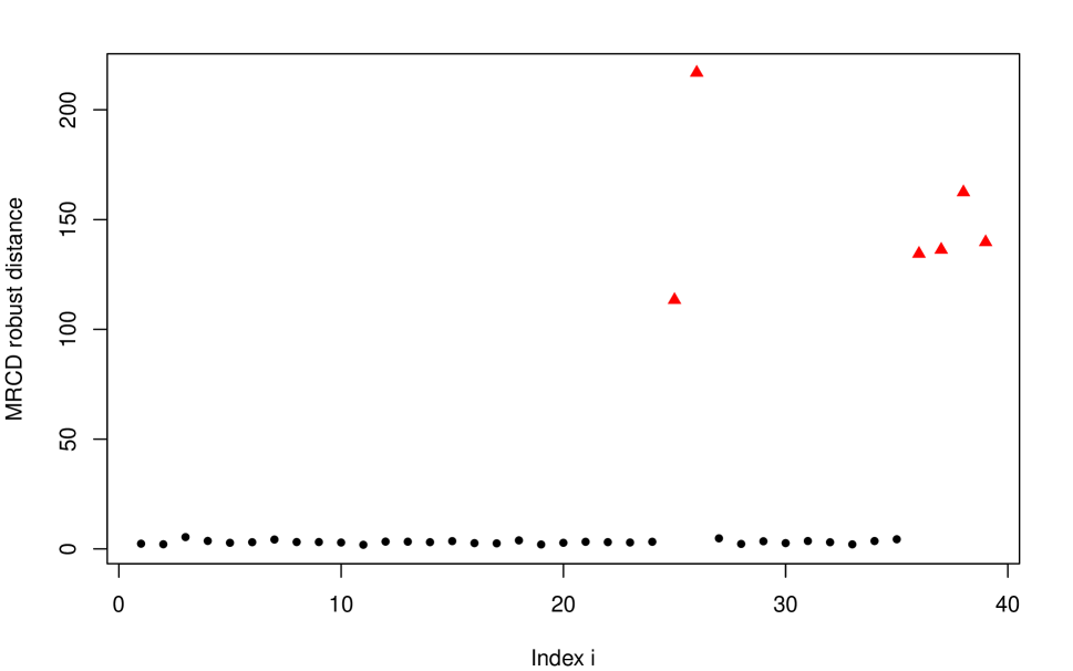
Figure 3: Robust distances of the octane data, based on the MRCD with $h=33$.

We then calculate the MRCD estimator with $h=33$, yielding $\rho=0.1149$. Figure 3 shows the corresponding robust distances

$$RD(\boldsymbol{x}_{i})=\sqrt{(\boldsymbol{x}_{i}-\mathbf{m}_{MRCD})^{\prime}\mathbf{K}_{MRCD}^{-1}(\boldsymbol{x}_{i}-\mathbf{m}_{MRCD})}$$ (20)

where $\mathbf{m}_{MRCD}$ and $\mathbf{K}_{MRCD}$ are the MRCD location and scatter estimates of (12). The flagged outliers (red triangles) stand out, showing the MRCD has correctly identified the 6 samples with added ethanol.

5.2 Murder rate data

Khan et al. (2007) regress the murder rate per 100,000 residents in the $n=50$ states of the US in 1980 on 25 demographic predictors, and mention that graphical tools reveal one clear outlier.

For lower-dimensional data, Rousseeuw et al. (2004) applied the MCD estimator to the response(s) and predictors together to robustly estimate a multivariate regression. Here we investigate whether for high-dimensional data the same type of analysis can be carried out based on the MRCD. In the murder rate data this yields a total of 26 variables.

As for the octane data, we compute the MRCD estimates for the candidate range of $h$. In Figure 5 we see a big jump in the objective function when going from $h=49$ to $h=50$. But in the plot of the Frobenius distance between successive MRCD scatter matrices (Figure 5) we see evidence of four outliers, which lead to a substantial change in the MRCD when included in the subset.

Figure 4: Murder rate data: MRCD objective value (10) for different values of $h$.

Figure 5: Murder rate data: Frobenius distance between MRCD scatter matrices on standardized data for $h-1$ and $h$.

As a conservative choice we set $h=44$, which allows for up to 6 outliers. We then partition the MRCD scatter matrix on all 26 variables as follows:

$$\mathbf{K}_{MRCD}=\left(\begin{array}[]{cc}\mathbf{K}_{xx}&\mathbf{K}_{xy}\\ \mathbf{K}_{xy}&\mathbf{K}_{yy}\end{array}\right),$$

where $x$ stands for the vector of predictors and $y$ is the response variable. The resulting estimate of the slope vector is then

$$\hat{\beta}_{MRCD}=\mathbf{K}_{xx}^{-1}\mathbf{K}_{xy}\;.$$

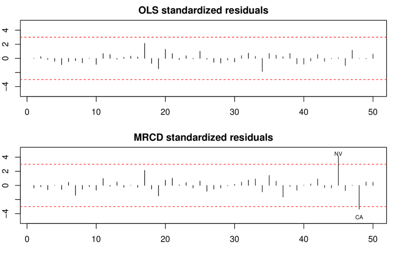
Figure 6: Standardized residuals of regressing the murder rate on demographic variables.

The resulting standardized residuals are shown in Figure 6. The standardized residuals obtained with OLS indicate that there are no outliers in the data since all residuals are clearly between the cut-off lines. In contrast, the MRCD regression flags Nevada as an upwards outlier and California as a downwards outlier. It is therefore recommended to study these states in more detail. Note that both states have very small residuals when using OLS. This is a clear example of the well known masking effect: classical methods can be affected by outliers so strongly that the resulting fitted model does not allow to detect the deviating observations.

Finally, we note that MRCD regression can be plugged into existing robust algorithms for variable selection, which avoids the limitation mentioned in Khan et al. (2007) that “a robust fit of the full model may not be feasible due to the numerical complexity of robust estimation when [the dimension] $d$ is large (e.g., $d$ $\geq$ 200) or simply because $d$ exceeds the number of cases, $n$.” The MRCD could be used in such situations because its computation remains feasible in higher dimensions.

6 Concluding remarks

In this paper we generalized the Minimum Covariance Determinant (MCD) estimation approach of Rousseeuw (1985) to higher dimensions, by regularizing the sample covariance matrices of subsets before minimizing their determinant. The resulting Minimum Regularized Covariance Determinant (MRCD) estimator is well-conditioned by construction, even when $p>n$, and preserves the good robustness of the MCD. We constructed a fast algorithm for the MRCD by generalizing the C-step used by the MCD, and proving that this generalized C-step is guaranteed to reduce the covariance determinant. We verified the performance of the MRCD estimator in an extensive simulation study including both clean and contaminated data. The simulation study also confirmed that the MRCD can be interpreted as a generalization of the MCD. When $n$ is sufficiently large compared to $p$ and the MCD is well-conditioned, the regularization parameter in MRCD becomes zero and the MRCD estimate coincides with the MCD. Finally, we illustrated the use of the MRCD for outlier detection and robust regression on two fat data applications from chemistry and criminology, for which $p>n/2$.

We believe that the MRCD is a valuable addition to the tool set for robust multivariate analysis, especially in high dimensions. Thanks to the function CovMrcd in the R package rrcov of Todorov and Filzmoser (2009), practitioners and academics can easily implement our methodology in practice. We look forward to further research on its use in principal component analysis where the original MCD has proved useful (Croux and Haesbroeck, 2000; Hubert et al., 2005), and analogously in factor analysis (Pison et al., 2003), classification (Hubert and Van Driessen, 2004), clustering (Hardin and Rocke, 2004), multivariate regression (Rousseeuw et al., 2004), penalized maximum likelihood estimation (Croux et al., 2012) and other multivariate techniques. A further research topic is to study the finite sample distribution of the robust distances computed from the MRCD. Our experiments have shown that the usual chi-square and F-distribution results for the MCD distances (Hardin and Rocke, 2005) are no longer good approximations when $p$ is large relatively to $n$. A better approximation would be useful for improving the accuracy of the MRCD by reweighting.

Appendix A: Proof of Theorem 1 Generate a $p$-variate sample $\mathbf{Z}$ with $p+1$ points for which $\mathbf{\Lambda}=\frac{1}{p+1}\sum_{j=1}^{p+1}(\boldsymbol{z}_{i}-\overline{z})(\boldsymbol{z}_{i}-\overline{z})^{\prime}$ is nonsingular and$\overline{z}=\frac{1}{p+1}\sum_{j=1}^{p+1}\boldsymbol{z}_{i}$. Then $\tilde{\boldsymbol{z}}_{i}=\mathbf{\Lambda}^{-1/2}(\boldsymbol{z}_{i}-\overline{z})$ has mean zero and covariance matrix $\mathbf{I}_{p}$. Now compute $\boldsymbol{y}_{i}=\mathbf{T}^{1/2}\tilde{\boldsymbol{z}}_{i}\;$, hence $\mathbf{Y}$ has mean zero and covariance matrix $\mathbf{T}$.

Next, create the artificial dataset

$$\tilde{\mathbf{X}}^{1}=\left(w_{1}(\boldsymbol{x}^{1}_{1}-\mathbf{m}_{1}),\ldots,w_{h}(\boldsymbol{x}^{1}_{h}-\mathbf{m}_{1}),w_{h+1}\boldsymbol{y}_{1},\ldots,w_{k}\boldsymbol{y}_{p+1}\right)$$

with $k=h+p+1$ points, where $\boldsymbol{x}^{1}_{1},\ldots,\boldsymbol{x}^{1}_{h}$ are the members of $H_{1}$. The factors $w_{i}$ are given by

$$w_{i}=\left\{\begin{array}[]{cl}\sqrt{k(1-\rho)/h}&\;\;\;\mbox{for}\ i=1,\ldots,h\\ \sqrt{k\rho/(p+1)}&\;\;\;\mbox{for}\ i=h+1,\ldots,k\;\;.\end{array}\right.$$

The mean and covariance matrix of $\mathbf{\tilde{X}}^{1}$ are then

$$\frac{1}{k}\sum_{i=1}^{k}\boldsymbol{\tilde{x}}^{1}_{i} =\sqrt{\frac{1-\rho}{kh}}\sum_{i=1}^{h}(\boldsymbol{x}^{1}_{i}-\mathbf{m}_{1})+\sqrt{\frac{\rho}{k(p+1)}}\sum_{j=1}^{p+1}\boldsymbol{y}_{j}=0$$

and

$$\frac{1}{k}\sum_{i=1}^{k}\boldsymbol{\tilde{x}}^{1}_{i}(\boldsymbol{\tilde{x}}^{1}_{i})^{\prime} =\frac{1-\rho}{h}\sum_{i=1}^{h}(\boldsymbol{x}^{1}_{i}-\mathbf{m}_{1})(\boldsymbol{x}^{1}_{i}-\mathbf{m}_{1})^{\prime}+\frac{\rho}{p+1}\sum_{j=1}^{p+1}\boldsymbol{y}_{j}\boldsymbol{y}^{\prime}_{j}$$

$$=(1-\rho)\mathbf{S}_{1}+\rho\mathbf{T}=\mathbf{K}_{1}\;\;.$$

The regularized covariance matrix $\mathbf{K}_{1}$ is thus the actual covariance matrix of the combined data set $\mathbf{\tilde{X}}^{1}\;$. Analogously we construct

$$\tilde{\mathbf{X}}^{2}=\left(w_{1}(\boldsymbol{x}^{2}_{1}-\mathbf{m}_{2}),\ldots,w_{h}(\boldsymbol{x}^{2}_{h}-\mathbf{m}_{2}),w_{h+1}\boldsymbol{y}_{1},\ldots,w_{k}\boldsymbol{y}_{p+1}\right)$$

where $\boldsymbol{x}^{2}_{1},\ldots,\boldsymbol{x}^{2}_{h}$ are the members of $H_{2}\;$. $\tilde{\mathbf{X}}_{2}$ has zero mean and covariance matrix $\mathbf{K}_{2}=(1-\rho)\mathbf{S}_{2}+\rho\mathbf{T}\;$.

Denote $d_{\mathbf{K}_{1}}(\boldsymbol{\tilde{x}})=\boldsymbol{\tilde{x}^{\prime}}(\mathbf{K}_{1})^{-1}\boldsymbol{\tilde{x}}$. We can then prove that:

$$\frac{1}{k}\sum_{i=1}^{h}d_{\mathbf{K}_{1}}(\boldsymbol{\tilde{x}}^{2}_{i}) =\frac{1-\rho}{h}\sum_{i=1}^{h}d_{\mathbf{K}_{1}}(\boldsymbol{x}^{2}_{i}-\mathbf{m}_{2})$$ (21)

$$\leq\frac{1-\rho}{h}\sum_{i=1}^{h}d_{\mathbf{K}_{1}}(\boldsymbol{x}^{2}_{i}-\mathbf{m}_{1})$$ (22)

$$\leq\frac{1-\rho}{h}\sum_{i=1}^{h}d_{\mathbf{K}_{1}}(\boldsymbol{x}^{1}_{i}-\mathbf{m}_{1})$$ (23)

$$=\frac{1}{k}\sum_{i=1}^{h}d_{\mathbf{K}_{1}}(\mathbf{\tilde{x}}^{1}_{i})$$ (24)

in which the second inequality (23) is the condition (18).

The first inequality (22) can be shown as follows. Put $\boldsymbol{z}_{i}=(\mathbf{K}_{1})^{-1/2}\boldsymbol{x}^{2}_{i}$ and $\tilde{\boldsymbol{z}}=(\mathbf{K}_{1})^{-1/2}\mathbf{m}_{1}$ and note that $\overline{\boldsymbol{z}}=(\mathbf{K}_{1})^{-1/2}\mathbf{m}_{2}$ is the average of the $\boldsymbol{z}_{i}$. Then (22) becomes

$$\sum_{i=1}^{h}\|\boldsymbol{z}_{i}-\overline{\boldsymbol{z}}\|^{2}\leq\sum_{i=1}^{h}\|\boldsymbol{z}_{i}-\tilde{\boldsymbol{z}}\|^{2},$$

which follows from the fact that $\tilde{\boldsymbol{z}}$ is the unique minimizer of the least squares objective $\sum_{i=1}^{k}\|\boldsymbol{z}_{i}-c\|^{2}$, so (22) becomes an equality if and only if $\tilde{\boldsymbol{z}}=\overline{\boldsymbol{z}}$ which is equivalent to $\mathbf{m}_{2}=\mathbf{m}_{1}$.
It follows that

$$\sum_{i=1}^{k}d_{\mathbf{K}_{1}}(\boldsymbol{\tilde{x}}^{2}_{i}) =\sum_{i=1}^{h}d_{\mathbf{K}_{1}}(\boldsymbol{\tilde{x}}^{2}_{i})+\frac{\rho}{p+1}\sum_{j=1}^{p+1}d_{\mathbf{K}_{1}}(\boldsymbol{y}_{j})$$

$$\leq\sum_{i=1}^{h}d_{\mathbf{K}_{1}}(\boldsymbol{\tilde{x}}^{1}_{i})+\frac{\rho}{p+1}\sum_{j=1}^{p+1}d_{\mathbf{K}_{1}}(\boldsymbol{y}_{j})$$

$$=\sum_{i=1}^{k}d_{\mathbf{K}_{1}}(\boldsymbol{\tilde{x}}^{1}_{i})\;\;.$$

Now put

$$b=\frac{\sum_{i=1}^{k}d_{\mathbf{K}_{1}}(\boldsymbol{\tilde{x}}^{2}_{i})}{\sum_{i=1}^{k}d_{\mathbf{K}_{1}}(\boldsymbol{\tilde{x}}^{1}_{i})}\leq 1\;\;.$$

If we now compute distances relative to $b\mathbf{K}_{1}\;$, we find

$$\frac{1}{k}\sum_{i=1}^{k}d_{b\mathbf{K}_{1}}(\boldsymbol{\tilde{x}}^{2}_{i})=\frac{1}{b}\frac{1}{k}\sum_{i=1}^{k}d_{\mathbf{K}_{1}}(\boldsymbol{\tilde{x}}^{2}_{i})=\frac{1}{k}\sum_{i=1}^{k}d_{\mathbf{K}_{1}}(\boldsymbol{\tilde{x}}^{1}_{i})=\frac{1}{k}\sum_{i=1}^{k}(\boldsymbol{\tilde{x}}^{1}_{i})^{\prime}(\mathbf{K}_{1})^{-1}\boldsymbol{\tilde{x}}^{1}_{i}$$

$$=\frac{1}{k}\sum_{i=1}^{k}(\mathbf{K}_{1}^{-1/2}\boldsymbol{\tilde{x}}^{1}_{i})^{\prime}(\mathbf{K}_{1}^{-1/2}\boldsymbol{\tilde{x}}^{1}_{i})=\mbox{Trace}\left(\frac{1}{k}\sum_{i=1}^{k}(\mathbf{K}_{1}^{-1/2}\boldsymbol{\tilde{x}}^{1}_{i})^{\prime}(\mathbf{K}_{1}^{-1/2}\boldsymbol{\tilde{x}}^{1}_{i})\right)$$

$$=\mbox{Trace}\left((\mathbf{K}_{1})^{-1/2}\left(\frac{1}{k}\sum_{i=1}^{k}(\boldsymbol{\tilde{x}}^{1}_{i})(\boldsymbol{\tilde{x}}^{1}_{i})^{\prime}\right)(\mathbf{K}_{1})^{-1/2}\right)=\mbox{Trace}(\mathbf{I}_{p})=p\;\;.$$

From the theorem in Grübel (1988), it follows that $\mathbf{K}_{2}$ is the unique minimizer of $\mbox{det}(\mathbf{S})$ among all $\mathbf{S}$ for which $\frac{1}{k}\sum_{i=1}^{k}d_{\mathbf{S}}(\boldsymbol{\tilde{x}}^{2}_{i})=p$ (note that the mean of $\boldsymbol{\tilde{x}}^{2}_{i}$ is zero). Therefore

$$\det(\mathbf{K}_{2})\leq\det(b\mathbf{K}_{1})\leq\det(\mathbf{K}_{1})\;\;.$$

We can only have $\mbox{det}(\mathbf{K}_{2})=\det(\mathbf{K}_{1})$ if both of these inequalities are equalities. For the first, by   uniqueness we can only have equality if $\mathbf{K}_{2}=b\mathbf{K}_{1}$. For the second inequality, equality holds if and only if $b=1$. Combining both yields $\mathbf{K}_{2}=\mathbf{K}_{1}$. Moreover, $b=1$ implies that (22) becomes an equality, hence $\mathbf{m}_{2}=\mathbf{m}_{1}$. This concludes the proof of Theorem 1.

Appendix B: The OGK estimator

Maronna and Zamar (2002) presented a general method to obtain positive definite and approximately affine equivariant robust scatter matrices starting from a robust bivariate scatter measure. This method was applied to the bivariate covariance estimate of Gnanadesikan and Kettenring (1972). The resulting multivariate location and scatter estimates are called orthogonalized Gnanadesikan-Kettenring (OGK) estimates and are calculated as follows:

1. Let $m(.)$ and $s(.)$ be robust univariate estimators of location and scale.

2. Construct $\boldsymbol{y}_{i}=\boldsymbol{D}^{-1}\boldsymbol{x}_{i}$ for $i=1,\ldots,n$ with $\boldsymbol{D}=\text{diag}(s(X_{1}),\ldots,s(X_{p}))\;$.

3. Compute the ‘pairwise correlation matrix’ $\boldsymbol{U}$ of the variables of $\boldsymbol{Y}=(Y_{1},\ldots,Y_{p})\;$, given by $u_{jk}=1/4(s(Y_{j}+Y_{k})^{2}-s(Y_{j}-Y_{k})^{2})\;$. This $\boldsymbol{U}$ is symmetric but not necessarily positive definite.

4. Compute the matrix $\boldsymbol{E}$ of eigenvectors of $\boldsymbol{U}$ and

   1. project the data on these eigenvectors, i.e. $\boldsymbol{V}=\boldsymbol{Y}\boldsymbol{E}\;$;

   2. compute ‘robust variances’ of $\boldsymbol{V}=(V_{1},\ldots,V_{p})\;$, i.e. $\boldsymbol{\Lambda}=\text{diag}(s^{2}(V_{1}),\ldots,s^{2}(V_{p}))\;$;

   3. set the $p\times 1$ vector $\hat{\boldsymbol{\mu}}(\boldsymbol{Y})=\boldsymbol{E}\boldsymbol{m}$ where $\boldsymbol{m}=(m(V_{1}),\ldots,m(V_{p}))^{T}\;$, and compute the positive definite matrix $\hat{\boldsymbol{\Sigma}}(\boldsymbol{Y})=\boldsymbol{E}\boldsymbol{\Lambda}\boldsymbol{E}^{T}\;$.

5. Transform back to $\boldsymbol{X}$, i.e. $\hat{\boldsymbol{\mu}}_{\textrm{OGK}}=\boldsymbol{D}\hat{\boldsymbol{\mu}}(\boldsymbol{Y})$ and $\hat{\boldsymbol{\Sigma}}_{\textrm{OGK}}=\boldsymbol{D}\hat{\boldsymbol{\Sigma}}(\boldsymbol{Y})\boldsymbol{D}^{T}\;$.

Step 2 makes the estimate location invariant and scale equivariant, whereas the next steps replace the eigenvalues of $\boldsymbol{U}$ (some of which may be negative) by positive numbers. In the simulation study and empirical analysis, we set $m(.)$ to the median and $s(.)$ to either the median absolute deviation or the Qn scale estimator. We use the implementation in the R package rrcov of Todorov and Filzmoser (2009).

Appendix C: The RMCD estimator

The RMCD as initially proposed by Croux et al. (2012) uses random subsets. Below we give its adaptation using deterministic subsets. We thank Christophe Croux and Gentiane Haesbrouck for their helpful guidelines in specifying the proposed detRMCD algorithm in which we follow closely the MRCD algorithm presented in Section 3. It uses the GLASSO algorithm of Friedman et al. (2008), as implemented in the package huge of Zhao et al. (2012).

—————————————————
(det)RMCD algorithm
—————————————————

1. Compute the standardized observations $\boldsymbol{u}_{i}$ as defined in (6) using the median and the Qn estimator for univariate location and scale.

2. Find the RMCD subset:

   1. Follow Subsection 3.1 in Hubert et al. (2012) to obtain six robust, well-conditioned initial location estimates $\boldsymbol{m}^{i}$ and scatter estimates $\mathbf{S}^{i}$ ($i=1,\ldots,6$). Use GLASSO to transform the scatter estimate into a precision matrix $\mathbf{P}^{i}$ and denote the corresponding regularization parameter by $\lambda^{i}$.

   2. Compute for each subset, the extended BIC criterion and set $\lambda$ to the $\lambda^{i}$ of the subset with lowest extended BIC criterion.

   3. For all initial subsets $H_{0}^{i}$, use $\lambda$ and repeat the generalized RMCD C-steps until convergence. Denote the resulting subsets as $H^{i}\;$.

   4. Let $H_{RMCD}$ be the subset with largest GLASSO objective function (penalized log-likelihood) among the candidate subsets.

3. From $H_{RMCD}$ compute the final RMCD estimates of location, scale and precision as in Croux et al. (2012).

References

- Agostinelli et al. (2015) Agostinelli, C., A. Leung, V. Yohai, and R. Zamar (2015). Robust estimation of multivariate location and scatter in the presence of cellwise and casewise contamination. Test 24(3), 441–461.
- Agulló et al. (2008) Agulló, J., C. Croux, and S. Van Aelst (2008). The multivariate least trimmed squares estimator. Journal of Multivariate Analysis 99, 311–338.
- Atkinson et al. (2004) Atkinson, A. C., M. Riani, and A. Cerioli (2004). Exploring multivariate data with the forward search. Springer-Verlag New York.
- Bartlett (1951) Bartlett, M. S. (1951). An inverse matrix adjustment arising in discriminant analysis. The Annals of Mathematical Statistics 22(1), 107–111.
- Boudt et al. (2012) Boudt, K., J. Cornelissen, and C. Croux (2012). Jump robust daily covariance estimation by disentangling variance and correlation components. Computational Statistics & Data Analysis 56(11), 2993–3005.
- Butler et al. (1993) Butler, R., P. Davies, and M. Jhun (1993). Asymptotics for the Minimum Covariance Determinant estimator. The Annals of Statistics 21(3), 1385–1400.
- Cator and Lopuhaä (2012) Cator, E. and H. Lopuhaä (2012). Central limit theorem and influence function for the MCD estimator at general multivariate distributions. Bernoulli 18(2), 520–551.
- Croux and Dehon (2010) Croux, C. and C. Dehon (2010). Influence functions of the Spearman and Kendall correlation measures. Statistical Methods & Applications 19(4), 497–515.
- Croux et al. (2012) Croux, C., S. Gelper, and G. Haesbroeck (2012). Regularized Minimum Covariance Determinant estimator. Mimeo.
- Croux and Haesbroeck (1999) Croux, C. and G. Haesbroeck (1999). Influence function and efficiency of the minimum covariance determinant scatter matrix estimator. Journal of Multivariate Analysis 71(2), 161–190.
- Croux and Haesbroeck (2000) Croux, C. and G. Haesbroeck (2000). Principal components analysis based on robust estimators of the covariance or correlation matrix: influence functions and efficiencies. Biometrika 87, 603–618.
- Esbensen et al. (1996) Esbensen, K., T. Midtgaard, and S. Schönkopf (1996). Multivariate Analysis in Practice: A Training Package. Camo As.
- Fan et al. (2008) Fan, J., Y. Fan, and J. Lv (2008). High dimensional covariance matrix estimation using a factor model. Journal of Econometrics 147, 186–197.
- Friedman et al. (2008) Friedman, J., T. Hastie, and R. Tibshirani (2008). Sparse inverse covariance estimation with the graphical lasso. Biostatistics 9(2), 432–441.
- Gnanadesikan and Kettenring (1972) Gnanadesikan, R. and J. Kettenring (1972). Robust estimates, residuals, and outlier detection with multiresponse data. Biometrics 28, 81–124.
- Grübel (1988) Grübel, R. (1988). A minimal characterization of the covariance matrix. Metrika 35(1), 49–52.
- Hardin and Rocke (2004) Hardin, J. and D. Rocke (2004). Outlier detection in the multiple cluster setting using the minimum covariance determinant estimator. Computational Statistics & Data Analysis 44, 625–638.
- Hardin and Rocke (2005) Hardin, J. and D. Rocke (2005). The distribution of robust distances. Journal of Computational and Graphical Statistics 14(4), 928–946.
- Hubert et al. (2008) Hubert, M., P. Rousseeuw, and S. Van Aelst (2008). High breakdown robust multivariate methods. Statistical Science 23, 92–119.
- Hubert et al. (2005) Hubert, M., P. Rousseeuw, and K. Vanden Branden (2005). ROBPCA: a new approach to robust principal components analysis. Technometrics 47, 64–79.
- Hubert et al. (2012) Hubert, M., P. Rousseeuw, and T. Verdonck (2012). A deterministic algorithm for robust location and scatter. Journal of Computational and Graphical Statistics 21(3), 618–637.
- Hubert and Van Driessen (2004) Hubert, M. and K. Van Driessen (2004). Fast and robust discriminant analysis. Computational Statistics and Data Analysis 45, 301–320.
- Ledoit and Wolf (2004) Ledoit, O. and M. Wolf (2004). A well-conditioned estimator for large-dimensional covariance matrices. Journal of Multivariate Analysis 88, 365–411.
- Khan et al. (2007) Khan, J., S. Van Aelst, and R. H. Zamar (2007). Robust linear model selection based on least angle regression. Journal of the American Statistical Association 102(480), 1289–1299.
- Lopuhaä and Rousseeuw (1991) Lopuhaä, H. and P. Rousseeuw (1991). Breakdown points of affine equivariant estimators of multivariate location and covariance matrices. The Annals of Statistics 19, 229–248.
- Maronna and Zamar (2002) Maronna, R. and R. H. Zamar (2002). Robust estimates of location and dispersion for high-dimensional datasets. Technometrics 44(4), 307–317.
- Todorov and Filzmoser (2009) Todorov, V. and P. Filzmoser (2009). An Object-Oriented Framework for Robust Multivariate Analysis. Journal of Statistical Software 32(3), 1–47.
- Öllerer and Croux (2015) Öllerer, V. and C. Croux (2015). Robust high-dimensional precision matrix estimation. In Modern Nonparametric, Robust and Multivariate Methods, pp. 325–350. Springer.
- Pison et al. (2003) Pison, G., P. Rousseeuw, P. Filzmoser, and C. Croux (2003). Robust factor analysis. Journal of Multivariate Analysis 84, 145–172.
- Rousseeuw (1984) Rousseeuw, P. (1984). Least median of squares regression. Journal of the American Statistical Association 79(388), 871–880.
- Rousseeuw (1985) Rousseeuw, P. (1985). Multivariate estimation with high breakdown point. In W. Grossmann, G. Pflug, I. Vincze, and W. Wertz (Eds.), Mathematical Statistics and Applications, Vol. B, pp. 283–297. Reidel Publishing Company, Dordrecht.
- Rousseeuw and Croux (1993) Rousseeuw, P. and C. Croux (1993). Alternatives to the median absolute deviation. Journal of the American Statistical Association 88(424), 1273–1283.
- Rousseeuw et al. (2012) Rousseeuw, P., C. Croux, V. Todorov, A. Ruckstuhl, M. Salibian-Barrera, T. Verbeke, M. Koller, and M. Maechler (2012). Robustbase: Basic Robust Statistics. R package version 0.92-3.
- Rousseeuw et al. (2004) Rousseeuw, P., S. Van Aelst, K. Van Driessen, and J. Agulló (2004). Robust multivariate regression. Technometrics 46, 293–305.
- Rousseeuw and Van Driessen (1999) Rousseeuw, P. and K. Van Driessen (1999). A fast algorithm for the Minimum Covariance Determinant estimator. Technometrics 41, 212–223.
- Rousseeuw and Van Zomeren (1990) Rousseeuw, P. and B. Van Zomeren (1990). Unmasking multivariate outliers and leverage points. Journal of the American Statistical Association 85(411), 633–639.
- SenGupta (1987) SenGupta, A. (1987). Tests for standardized generalized variances of multivariate normal populations of possibly different dimensions. Journal of Multivariate Analysis 23(2), 209–219.
- Sherman and Morrison (1950) Sherman, J. and W. J. Morrison (1950). Adjustment of an inverse matrix corresponding to a change in one element of a given matrix. The Annals of Mathematical Statistics 21(1), 124–127.
- Won et al. (2013) Won, J.-H., J. Lim, S.-J. Kim, and B. Rajaratnam (2013). Condition-number-regularized covariance estimation. Journal of the Royal Statistical Society: Series B (Statistical Methodology) 75(3), 427–450.
- Woodbury (1950) Woodbury, M. A. (1950). Inverting modified matrices. Memorandum report 42, 106.
- Zhao et al. (2012) Zhao, T., H. Liu, K. Roeder, J. Lafferty and L. Wasserman (2012). The huge package for high-dimensional undirected graph estimation in R. Journal of Machine Learning Research 13, 1059–1062.