Instability of the non-Fermi liquid state of the Sachdev-Ye-Kitaev Model

Abstract

We study a series of perturbations on the Sachdev-Ye-Kitaev (SYK) model. We show that the maximal chaotic non-Fermi liquid phase described by the ordinary $q=4$ SYK model has marginally relevant/irrelevant (depending on the sign of the coupling constants) four-fermion perturbations allowed by symmetry. Changing the sign of one of these four-fermion perturbations leads to a continuous chaotic-nonchaotic quantum phase transition of the system accompanied by a spontaneous time-reversal symmetry breaking. Starting with the SYK_q model with a $q-$fermion interaction, similar perturbations can lead to a series of new fixed points with continuously varying exponents.

I Introduction

Non-Fermi liquids usually occur at quantum critical points of itinerant electron systems Hertz (1976); Millis (1993); Löhneysen et al. (2007). Strong correlation and quantum critical fluctuation often make it challenging to study the non-fermi liquids through the standard diagrammatic approach, and various expansion methods have been developed for that purpose Lee (2009); Mross et al. (2010); Metlitski and Sachdev (2010a, b); Dalidovich and Lee (2013). Fortunately, there exist some exactly soluble models for non-Fermi liquid states which do not rely on perturbation theory. In 1993, Sachdev and Ye constructed one such example in $(0+1)d$ Sachdev and Ye (1993), which was reintroduced in a modified version lately by Kitaev Kitaev (2015). This model is now known as the Sachdev-Ye-Kitaev (SYK) model. The SYK model is a $(0+1)d$ system that consists of $N$ Majorana fermions with $q$-fermion random interactions. When $q=2$, the model is simply $N$ Majorana fermions with only random hopping terms, which can be solved completely using the random matrix theory. The $q=4$ SYK model (hereafter labelled as SYK₄ model) is most thoroughly studied. Its Hamiltonian is given by

$$H_{\text{SYK}_{4}}=\sum_{ijkl}\frac{J_{ijkl}}{4!}\chi_{i}\chi_{j}\chi_{k}\chi_{l},$$ (1)

where $\chi_{i,j,k,l}$ are Majorana fermion operators with index $i,j,k,l=1\cdots N$, and $J_{ijkl}$ is a fully anti-symmetric tensor whose each entry is drawn from a Gaussian distribution with zero mean and variance $\overline{J_{ijkl}^{2}}=3!J_{4}^{2}/N^{3}$. With large $N$ and low temperature, the SYK₄ model can be solved exactly via saddle point equations and exhibits an emergent conformal symmetry. The scaling dimension of the Fermion operator is $\Delta_{f}=1/4$, which suggests a non-Fermi liquid behavior without quasi-particle excitations Kitaev (2015); Maldacena and Stanford (2016).

Furthermore, the exact solution also suggests that the SYK₄ model is maximally chaotic, in the sense that its Lyapunov exponent Kitaev (2015); Maldacena and Stanford (2016), a measure of quantum chaos, saturates the universal upper bound established in Ref. Maldacena et al., 2016a. The saturation of the universal upper bound is also a feature of black holes. In fact, the exact solution also indicates that the SYK₄ model should indeed be holographically dual to a gravity theory Sachdev (2010, 2015); Polchinski and Rosenhaus (2016); Jensen (2016); Engelsöy et al. (2016); Maldacena and Stanford (2016); Maldacena et al. (2016b). All SYK_q models share the properties such as maximally chaotic non-Fermi liquid ground states (for $q>2$), emergent conformal symmetry at large-$N$ , etc. Many other aspects of the SYK model, including the numerical simulations, generalizations to models with higher symmetry, and higher dimensions, have been investigated recently Georges et al. (2001); You et al. (2016); Fu and Sachdev (2016); Cotler et al. (2016); García-García and Verbaarschot (2016); Sachdev (2015); Fu et al. (2016); Gu et al. (2016); Davison et al. (2016); Witten (2016); Klebanov and Tarnopolsky (2016); Turiaci and Verlinde (2017); Banerjee and Altman (2016); Gross and Rosenhaus (2016); Krishnan et al. (2016).

One peculiar feature of the SYK_q model with $q>2$ is that, in the large $N$ limit, the chaotic non-Fermi liquids all have finite entropy density even when the temperature approaches zero Georges et al. (2001); Sachdev (2015); Kitaev (2015); Maldacena and Stanford (2016). One might conjecture directly that the system has instabilities towards states with lower (or zero) zero-temperature entropy density upon perturbations. Indeed, in experimental systems, the non-Fermi liquid state at a quantum critical point is usually buried in a dome of ordered phase with spontaneous symmetry breaking at low temperature Metlitski et al. (2015). One usual scenario is the emergence of a superconducting dome around the quantum critical point, which occurs in cuprates, pnictides superconductors, and also some heavy fermion systems. Thus it is meaningful to ask whether the SYK_q model, especially the SYK₄ model is instable against spontaneous symmetry breaking. Or in other words, the SYK₄ model could be the parent state of ordered phases at the infrared .

In this paper, we study a class of perturbations on the SYK_q models. We will concentrate mostly on the case with $q=4$. Obviously, the non-Fermi liquid at the SYK₄ fixed point will be unstable against the SYK₂ perturbation. However, the SYK₄ has a time-reversal symmetry, under which all fermion bilinears are odd. The time-reversal symmetry $\mathcal{T}$ forbids perturbations like the SYK₂ term. Thus we only consider four-fermion terms which are symmetric under $\mathcal{T}$. As we will show, the non-Fermi liquid SYK₄ model is instable against a series of four-fermion interactions that preserve all the symmetries, and the system flows to a state with spontaneous breaking of $\mathcal{T}$.

A similar analysis can be generalized to the SYK_q non-Fermi liquid with $q>4$ perturbed by the four-Fermion interactions we design. Interestingly, the four fermion interactions can drive the SYK_q model to a series of new stable fixed points with conformal symmetry.

II A perturbed $q=4$ SYK model

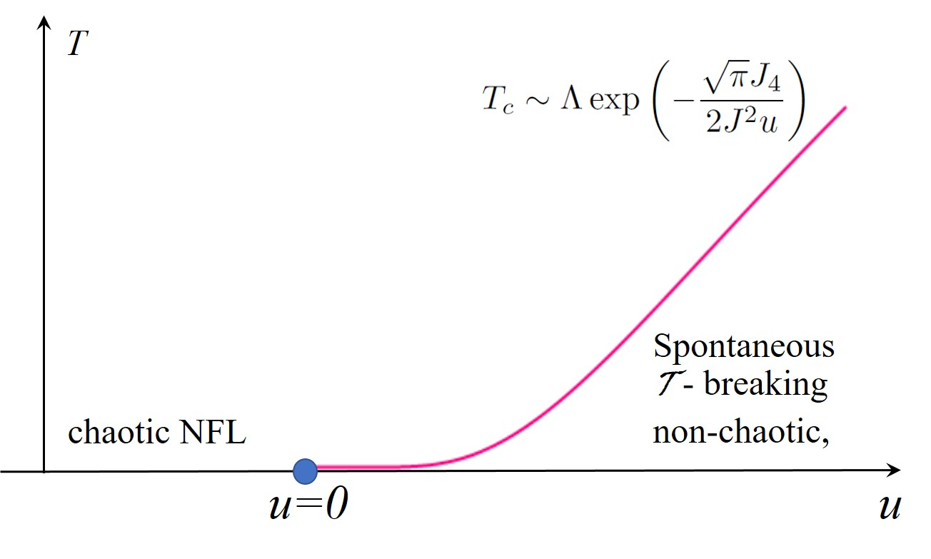
Figure 1: The phase diagram of Eq. 2.

The goal of the first section is to study the following generalized SYK model:

$$H=\frac{J_{ijkl}}{4!}\chi_{i}\chi_{j}\chi_{k}\chi_{l}+\frac{u}{2}C_{ij}C_{kl}\chi_{i}\chi_{j}\chi_{k}\chi_{l}$$ (2)

Both $J_{ijkl}$ and $C_{ij}$ are anti-symmetric random tensors drawn from a gaussian distribution. We choose the following normalization for $J_{ijkl}$ and $C_{ij}$:

$$\overline{J_{ijkl}}=0, \ \ \ N^{3}\overline{J_{ijkl}^{2}}=3!J_{4}^{2}$$

$$\overline{C_{ij}}=0, \ \ \ N^{2}\overline{C_{ij}C_{kl}}=J^{2}(\delta_{ik}\delta_{jl}-\delta_{il}\delta_{jk}).$$ (3)

Note that $J_{4}$ has the dimension of energy, while $J$ has the dimension of (energy)^1/2. The results of this section is summarized in phase diagram Fig. 1.

The two terms in Eq. 2 have the same symmetry: the time-reversal symmetry $\mathcal{T}$ which acts as $\chi_{j}\rightarrow\chi_{j}$, $i\rightarrow-i$ (it is the same time-reversal symmetry of the boundary states of the topological superconductor in the BDI class Kitaev (2009); Schnyder et al. (2009); Ryu et al. (2010)), and a statistical O($N$) symmetry. We will demonstrate that, by tuning $u$ from negative to positive, the system goes through a continuous phase transition from a chaotic phase to a nonchaotic phase. The critical properties of this transition are analogous to that of the Kosterlitz-Thouless transition, with exponent $\nu=+\infty$.

II.1 The $u-$term

Before we study Eq. 2, let us start with the Hamiltonian with only the second term:

$$H^{\prime}=\frac{u}{2}C_{ij}C_{kl}\chi_{i}\chi_{j}\chi_{k}\chi_{l}.$$ (4)

This Hamiltonian can be written as $H^{\prime}=-u\hat{b}^{2}/2$, with $\hat{b}=iC_{jk}\chi_{j}\chi_{k}$. Since $\hat{b}$ commutes with $H^{\prime}$, it is a conserved quantity. Thus every eigenstate of $H^{\prime}$ is an eigenstate of $\hat{b}$ with eigenvalue $b$. When $u>0$, the ground state of $H^{\prime}$ has the maximum eigenvalue of $\hat{b}$.

Now we can view $\hat{b}$ as a quadratic fermion Hamiltonian with random hopping. To maximize $\hat{b}$, the system fills all the negative (or positive) eigenvalues of the single fermion energy level $\varepsilon_{l}$, and $\mathrm{Max}[|b|]=|\sum\varepsilon_{l}|$ with $\varepsilon_{l}<0$.

The single particle energy levels $\varepsilon_{l}$ are the eigenvalues of the random Hermitian matrix $iC$. Based on the semi-circle law, the average number of eigenvalues of $iC$ in $(\varepsilon,\varepsilon+d\varepsilon)$ is given by $\rho(\varepsilon)d\varepsilon$ with

$$\rho(\varepsilon)=\frac{N^{2}}{2\pi J^{2}}\sqrt{\frac{4J^{2}}{N}-\varepsilon^{2}}.$$ (5)

Then we can obtain the average value of $\mathrm{Max}[|b|]$ as

$$\mathrm{Max}[|b|]=\Bigg{|}\int_{\varepsilon<0}d\varepsilon\varepsilon\rho(\varepsilon)\Bigg{|}=\frac{4JN^{\frac{1}{2}}}{3\pi}.$$ (6)

Therefore, the average ground state energy of $H^{\prime}$ is $E_{0}(H^{\prime})=-\frac{16uJ^{2}N}{9\pi^{2}}$. Thus just like the ordinary SYK model, $H^{\prime}$ normalized as in Eq. II is an order-$N$ term.

For $u<0$, all states with $b=0$ are ground states, and $b=0$ is a very “loose” condition. We will argue that $H^{\prime}$ with $u<0$ behaves like a completely free system with zero Hamiltonian. The (many-body) spectrum of $\hat{b}$ is given by $b=\sum_{\varepsilon_{l}>0}\varepsilon_{l}n_{l}$, where the occupation number $n_{l}=\pm 1$. This expression of $b$ is similar to an $\frac{N}{2}$-step random walk centered around $0$. The distribution of $b$ should therefore be Gaussian. The standard deviation $\sigma_{b}$ of this “random walk” is given by

$$\sigma_{b}^{2}=\sum_{\varepsilon_{l}>0}\varepsilon_{l}^{2}=\frac{1}{2}\text{Tr}\left((iC)^{\dagger}(iC)\right)=\sum_{i<j}|C_{ij}|^{2}=\frac{N-1}{2N}J^{2}.$$ (7)

The (many-body) density of states of $\hat{b}$ can be then approximated by

$$\rho(b)=2^{\frac{N}{2}}\sqrt{\frac{N}{\pi(N-1)J^{2}}}e^{-\frac{Nb^{2}}{(N-1)J^{2}}},$$ (8)

namely the number of eigenvalues of $\hat{b}$ in $(b,b+db)$ is given by $\rho(b)db$. The expression $\rho(b)$ of the density of states $\hat{b}$ is most accurate near $b=0$, which is exactly the region of interest when $u<0$. We can now calculate the partition function

$$\mathcal{Z}=\int db\rho(b)e^{\beta ub^{2}}=2^{\frac{N}{2}}\frac{1}{\sqrt{1+\beta|u|\frac{N-1}{N}J^{2}}}.$$ (9)

The entropy density $\mathcal{S}$ can be written as $\mathcal{S}=\frac{1}{N}\left(\log\mathcal{Z}-\beta\frac{\partial}{\partial\beta}\log\mathcal{Z}\right)$. Interestingly, we notice that, for any fixed $\beta$,

$$\lim_{N\rightarrow\infty}\mathcal{S}=\frac{1}{2}\log 2.$$ (10)

Therefore, if we take the large $N$ limit first before we take $\beta\rightarrow\infty$, we will conclude that the “ground state” entropy density is given by $\frac{1}{2}\log 2$. Such an entropy density is exactly the same as the system with zero Hamiltonian. Therefore, we argue that the system with $u<0$ behaves like a completely free system with zero Hamiltonian. Using the partition function, we can also calculate the specific heat of $H^{\prime}$ with $u<0$:

$$c_{v}=-\beta\frac{dS}{d\beta}=\frac{1}{2N}\left(\frac{\frac{N-1}{N}|u|J^{2}\beta}{1+\frac{N-1}{N}|u|J^{2}\beta}\right)^{2}.$$ (11)

II.2 Renormalization Group of $u$

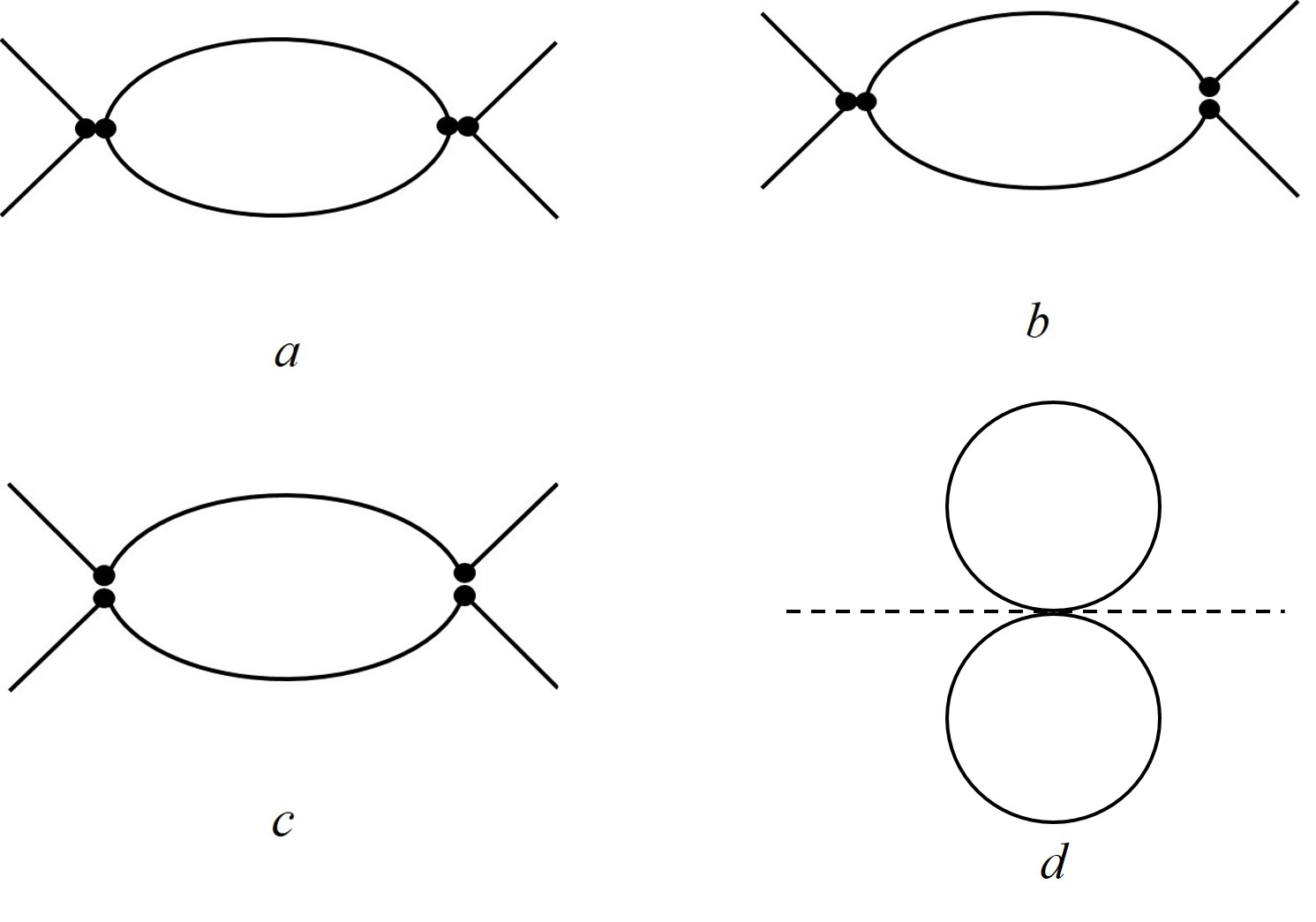
Figure 2: ($a$), ($b$), ($c$), the diagrams that we consider for the leading order RG for the coupling constant $u$ in Eq. 2. Only diagram ($a$) contributes in the large$-N$ limit. ($d$), the leading order RG for $u$ in Eq. 17, which is equivalent to ($a$), the solid and dashed lines are fermion and boson Green’s functions.

When $u$ is treated as a perturbation in Eq. 2, power counting indicates that it is a marginal perturbation at the SYK₄ fixed point. Now we perform a perturbative renormalization group calculation for $u$. We evaluate the fermion Green’s function at the SYK₄ fixed point:

$$G(\tau)=\left(\frac{1}{4\pi}\right)^{1/4}\frac{\mathrm{sgn}(\tau)}{|J_{4}\tau|^{1/2}},\ \ \ \ \ \ \ G(i\omega)=\pi^{1/4}\frac{i\mathrm{sgn}(\omega)}{|J_{4}\omega|^{1/2}}.$$ (12)

The diagram Fig. 2$a$ leads to the following beta function for $u$:

$$\beta(u)=\frac{du}{d\ln l}=\frac{2}{\sqrt{\pi}}\frac{1}{J_{4}}\sum_{i,j}|C_{ij}|^{2}u^{2}=\frac{2J^{2}}{\sqrt{\pi}J_{4}}u^{2}.$$ (13)

Here we have replaced $\sum_{i,j}|C_{ij}|^{2}$ by $J^{2}$, which is consistent with the distribution of $C_{ij}$, in the large $N$ limit.

Diagrams Fig. 2$b$ and $c$ will contribute at the subleading order of $1/N$. For example, Fig. 2$b$ will generate a term $\sim\sum_{m,n}C_{im}C_{mn}C_{nj}C_{kl}u^{2}\chi_{i}\chi_{j}\chi_{k}\chi_{l}$. This term is subleading in $1/N$ counting after disorder average.

The beta function indicates that the $H^{\prime}$ perturbation with $u>0$ ($u<0$) is marginally relevant (marginally irrelevant) at the SYK₄ fixed point. If we start with a small perturbation $u>0$, the RG equation implies that it will become order 1 at the energy scale $\tilde{\Lambda}$ where

$$\tilde{\Lambda}\sim\Lambda\exp\left(-\frac{\sqrt{\pi}J_{4}}{2J^{2}u}\right).$$ (14)

$\Lambda$ is the UV cut-off of the RG that we can roughly take as $\Lambda\sim J_{4}$. The standard scaling relation between the energy scale (mass gap) and the tuning parameter $r$ away from a critical point $r_{c}$ is $\tilde{\Lambda}\sim|r-r_{c}|^{\nu}$, thus the quantum phase transition led by tuning $u$ across zero has exponent $\nu=+\infty$, which is analogous to the Kosterlitz-Thouless transition Kosterlit and Thouless (1973).

This RG analysis predicts that the SYK model, although describes a non-Fermi liquid state, actually has similar instabilities as the ordinary Fermi liquid: there exists symmetry allowed four fermion terms that are marginally relevant/irreleavant depending on their sign. When $u$ is marginally relevant, our mean field solution in the next subsection (and the analysis of $H^{\prime}$ in the previous subsection) suggests that the fate of the SYK model is also similar to the ordinary Fermi liquid: the system develops long range correlation $\langle\hat{b}(0)\ \hat{b}(\tau)\rangle$, where $\hat{b}$ is the fermion-bilinear operator defined in the previous subsection. The physics here is analogous to the condensation of Cooper pair of the ordinary Fermi liquid theory.

The effective action of Eq. 2 after a Hubbard-Stratonovich transformation reads

$$\mathcal{S}_{eff} = \int d\tau\frac{1}{2}\sum_{i}\chi_{i}\partial_{\tau}\chi_{i}+\sum_{ijkl}\left\{\frac{J_{ijkl}}{4!}\chi_{i}\chi_{j}\chi_{k}\chi_{l}+\frac{u}{2}C_{ij}C_{kl}\chi_{i}\chi_{j}\chi_{k}\chi_{l}\right\}$$ (15)

$$= \int d\tau\left(\frac{1}{2}\chi_{i}\partial_{\tau}\chi_{i}+\frac{u}{2}b^{2}-iuC_{jk}b\chi_{j}\chi_{k}\right)+\frac{J_{ijkl}}{4!}\chi_{i}\chi_{j}\chi_{k}\chi_{l}$$ (16)

The Hubbard-Stratonovich field $b$ is a real field. Einstein summation convention is assumed in all the equations. The indices are summed from $1$ to $N$ with the constraint that different indices cannot take the same value. Now we can perform disorder average on $J_{ijkl}$ and $C_{jk}$ with the distribution Eq. II. Assuming everything is replica diagonal (justification of this assumption will be given in section IV), the disorder-averaged action is equivalent to the following form:

$$\mathcal{S}_{eff} = \int d\tau\frac{1}{2}\chi_{i}\partial_{\tau}\chi_{i}+\frac{u}{2}b^{2}-u^{2}\frac{J^{2}}{N^{2}}\int d\tau_{1}d\tau_{2}\ (b(\tau_{1})\ b(\tau_{2}))(\chi_{j}(\tau_{1})\chi_{j}(\tau_{2}))^{2}$$ (17)

$$-\frac{J_{4}^{2}}{8N^{3}}\int d\tau_{1}d\tau_{2}\ (\chi_{i}(\tau_{1})\chi_{i}(\tau_{2}))^{4}.$$

This disorder-averaged action has an explicit O($N$) symmetry, the fermion carries a vector representation of the O($N$).

The beta function for $u$ can also be computed based on Eq. 17. Fig. 2$d$ based on Eq. 17 makes the same contribution to the beta function as Fig. 2$a$. In the large$-N$ limit, the beta function Eq. 13 is actually exact. The higher order terms of the beta function can be ignored in the large$-N$ limit even when $u$ grows beyond order-1 (and hence becomes dominant) under the RG flow. For example the fermion wave function renormalization in Fig. 3 corresponds to a $u^{3}$ term in the beta function, and it carries a coefficient $1/N$. Other diagrams, such as the ladder diagrams for the four-point functions computed in Ref. Maldacena and Stanford, 2016, also contribute at the subleading $1/N$ order compared with Fig. 2$a$,$d$.

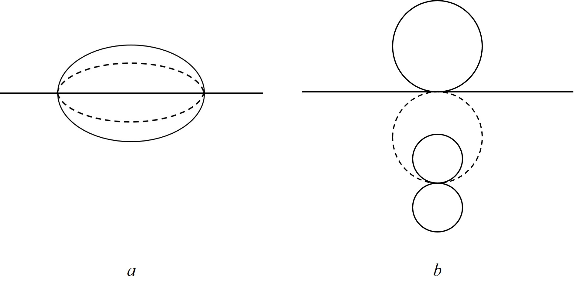
Figure 3: The fermion wave function renormalization based on Eq. 2 and Eq. 17 respectively. These diagrams correspond to a $u^{3}$ term in the beta function, and it carries a factor of $1/N$.

II.3 Mean field solution

We can introduce fermion Green’s function and Self-energy function $G$ and $\Sigma$ by inserting the following integral in the action ($G$ and $\Sigma$ are real fields):

$$\int\mathcal{D}\Sigma\mathcal{D}G\exp\left\{-\frac{N}{2}\Sigma(\tau_{1},\tau_{2})\left(G(\tau_{1},\tau_{2})-\frac{1}{N}\sum_{i}\chi_{i}(\tau_{1})\chi_{i}(\tau_{2})\right)\right\}$$ (18)

Then the action $S_{eff}$ is equivalent to:

$$\mathcal{S}_{eff} = -N\log\mathrm{Pf}\left(\partial_{\tau}-\Sigma\right)+\int d\tau\ \frac{u}{2}b^{2}-u^{2}J^{2}\int d\tau_{1}d\tau_{2}\ (b(\tau_{1})b(\tau_{2}))(G(\tau_{1},\tau_{2}))^{2}$$ (19)

$$-N\frac{J_{4}^{2}}{8}\int d\tau_{1}d\tau_{2}\ (G(\tau_{1},\tau_{2}))^{4}+N\int d\tau_{1}d\tau_{2}\ \frac{1}{2}\Sigma(\tau_{1},\tau_{2})G(\tau_{1},\tau_{2})$$

Since the $H^{\prime}$ term itself has long range correlation of $\hat{b}$, we expect that the phase with relevant $u$ perturbation also develops the long range correlation of $b(\tau)$. Since the ground state of $H^{\prime}$ has $b\sim N^{1/2}$, let us assume $\langle b(\tau_{1})b(\tau_{2})\rangle=Nw^{2}$, where $w$ takes order-1 value with no time dependence. Then we can derive the mean field equation for the Green’s function, the self-energy, and also $w$:

$$G(i\omega_{n})^{-1}=-i\omega_{n}-\Sigma(i\omega_{n})$$ (20)

$$\Sigma(\tau)=J_{4}^{2}G(\tau)^{3}+4u^{2}J^{2}w^{2}G(\tau)$$ (21)

$$\int d\tau\left(uJ^{2}G(\tau)^{2}-\frac{1}{2}\delta(\tau)\right)uw=0$$ (22)

The saddle point Eq. 22 has two possible solutions: $w=0$ or

$$\int d\tau\ G(\tau)^{2}=\frac{1}{2uJ^{2}}.$$ (23)

For the $w=0$ saddle point, these equations return to the saddle point equations for the pure $q=4$ SYK model. The system is in the chaotic non-Fermi liquid phase. However, when $w\neq 0$, in the low energy, the second term in Eq. 21 becomes dominant, and the system is effectively described by a random two fermion interaction and it is in a non-chaotic phase . In this phase, $G(\tau)$ will depend on the values of $w$, and we can self-consistently determine $w$ from Eq. 23. The chaotic-nonchaotic transition happens when $u$ is tuned from negative to positive through 0. When $u$ is negative, Eq. 23 has no solution and $w$ has to be $0$. For any positive $u$, at zero temperature there is always a solution with finite $w$. The state with long range correlation $\langle b(0)b(\tau)\rangle$ spontaneously breaks the time-reversal symmetry $\mathcal{T}:\chi_{j}\rightarrow\chi_{j}$.

There are two time scales in our problem, $\tau^{UV}_{2}\sim(uwJ)^{-1}$ and $\tau^{UV}_{4}\sim J_{4}^{-1}$. In the small $u$ limit, namely $\tau_{2}^{UV}\gg\tau_{4}^{UV}$, the contribution of the integral in Eq. 23 mainly comes from the region $\tau\in[\tau_{4}^{UV},\tau_{2}^{UV}]$, and in this region $G(\tau)$ takes the form of the ordinary SYK model:

$$\int d\tau\ G(\tau)^{2}\simeq\int_{\tau_{4}^{UV}}^{\tau_{2}^{UV}}d\tau\frac{2}{\sqrt{\pi}}\frac{1}{J_{4}\tau}=\frac{2}{\sqrt{\pi}J_{4}}\log(\frac{J_{4}}{uwJ})$$ (24)

Together with Eq. 23, we have

$$w\simeq\frac{J_{4}}{uJ}\exp\left(-\frac{\sqrt{\pi}J_{4}}{4uJ^{2}}\right).$$ (25)

This result is consistent with the observation that a positive $u$ is only marginally relevant. The size of the condensate is analogous to the superconductor gap of the BCS theory.

At finite $u$, the scale $\tilde{\Lambda}$ in Eq. 14 can be viewed as the critical temperature $T_{c}$ below which the system develops nonzero $w$ and hence spontaneously breaks time-reversal $\mathcal{T}$. Our numerical solution of the mean field equations Eq. 20,21,22 confirms the scaling between $T_{c}$ and $u$ (Fig. 4). In the numerical solution we have taken $J^{2}/J_{4}=1$. Our RG Eq. 14 predicts that $T_{c}\sim\exp(-\frac{\sqrt{\pi}}{2}\frac{1}{u})=\exp(-0.886/u)$, and our mean field solution gives $T_{c}\sim\exp(-0.897/u)$.

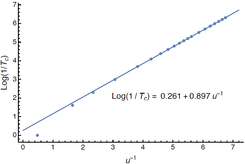
Figure 4: Transition temperature $T_{c}$ as a function of $u$ by numerically solving the mean field equations (20-22). This confirms the scaling relation in Eq. 14.

III Further generalized perturbations

Now let us consider a series of generalized Hamiltonians:

$$H=\mathrm{SYK}_{q}+H^{\prime},\ \ \ \ H^{\prime}=\frac{u}{2}\sum_{a=1}^{M}C^{a}_{ij}C^{a}_{kl}\chi_{i}\chi_{j}\chi_{k}\chi_{l},$$ (26)

with $M\sim N^{A}$. SYK_q is the generalized SYK model with a random $q-$fermion interaction, and $A\geq 0$. We first choose the following normalization of $C^{a}_{ij}$

$$N^{2}\ \overline{C^{a}_{ij}C^{b}_{kl}}=J^{2}\delta_{ab}(\delta_{ik}\delta_{jl}-\delta_{il}\delta_{jk}).$$ (27)

We still start with the beta function of $u$. If we evaluate the Green’s functions at the SYK_q fixed point, the beta function of $u$ reads

$$\beta(u)=\frac{du}{d\ln l}=(1-\frac{4}{q})u+Cu^{2}+\tilde{c}_{3}\frac{M}{N}u^{3}+\cdots$$ (28)

where $C>0$ is an order-1 constant.

III.1 cases with $A<1$

For $A<1$, we can keep just the linear and quadratic terms of the beta function, as all the higher order terms vanish in the large$-N$ limit, when $u$ is order-1 or smaller. For $A<1$ and $u>0$, $u$ is relevant at the SYK fixed point for $q>4$, and marginally relevant for $q=4$. We expect the system to behave similarly as the case with $M=1$ and $q=4$, namely the relevant $u$ perturbation drives the system into a nonchaotic phase with spontaneous $\mathcal{T}$ breaking: $\lim_{\tau\rightarrow\infty}\sum_{a}\langle b^{a}(0)\ b^{a}(\tau)\rangle\neq 0$, where $\hat{b}^{a}=iC^{a}_{jk}\chi_{j}\chi_{k}$. The same set of equations as Eq. 20,21,22 can be derived, and in this case $\sum_{a=1}^{M}\langle b^{a}(0)\ b^{a}(\tau)\rangle=Nw^{2}$, and $w$ is given by Eq. 25.

Exact diagonalization of the $H^{\prime}$ term in this case confirms our expectations. To detect the long range correlation of $\langle b^{a}(0)b^{a}(\tau)\rangle$, we measure the zero-frequency component of the boson spectral function. The spectral function is defined as

$$D(\omega)=\frac{1}{M}\sum_{a=1}^{M}\sum_{n}\big{|}\langle 0|\hat{b}^{a}|n\rangle\big{|}^{2}\delta(\omega-E_{n}+E_{0}),$$ (29)

where $E_{n}$ and $|n\rangle$ are eigenenergies and corresponding eigenstates of the Hamiltonian $H^{\prime}$, obtained from the exact diagonalization $H^{\prime}|n\rangle=E_{n}|n\rangle$ ($n=0,1,2,\cdots$). $n=0$ labels the ground state. The $C_{ij}^{a}$ normalization in Eq. 27 ensures that $\overline{\hat{b}^{a\dagger}\hat{b}^{a}}=1$ (the identity matrix) in the large $N$ limit, so that $D(\omega)$ has a well-defined thermodynamic limit. If the static correlation $D(\omega=0)$ remains finite in the thermodynamic limit $N\to\infty$, then the system will develop long range correlation and spontaneously break $\mathcal{T}$. The Fig. 5 shows the result of the static correlation $D(\omega=0)$ (in logarithmic scale) for different $N$ at $A=0.2$ and $u>0$. $\ln D(0)$ oscillates with $N$ in an eight-fold period due to the systematic change of random-matrix ensemble of $H^{\prime}$ as discussed in Ref. You et al., 2016. Apart from the oscillation, $D(\omega=0)$ remains at and converges to a finite level (roughly indicated by the dashed line in Fig. 5). Therefore our finite-sized calculation indeed supports a nonchaotic phase with spontaneous $\mathcal{T}$ breaking for the $A<1$ and $u>0$ case.

By contrast, for either $A>1$, or $A<1$ while $u<0$, ED shows $D(0)$ decreases rapidly with increasing $N$ (Fig. 6).

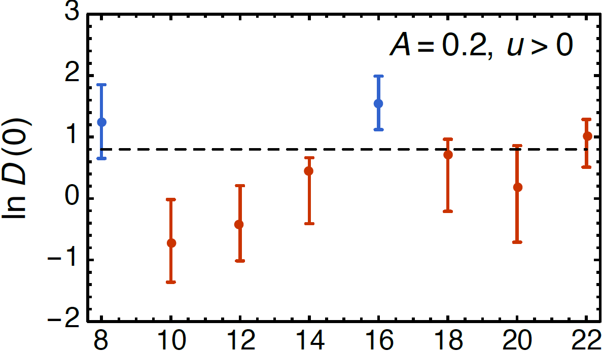
Figure 5: The logarithmic static correlation $\ln D(0)$ v.s. the fermion number $N$ for the case of $u>0$ and $A=0.2$. The error bar shows the statistical deviation over different random realizations of the coefficient $C_{ij}^{a}$. When $N\text{ mod }8=0$, $D(\omega=0)$ vanishes exactly, so we use the finite frequency extrapolation to obtain the static correlation $D(0)=\lim_{\omega\to 0}D(\omega)$ in these cases.

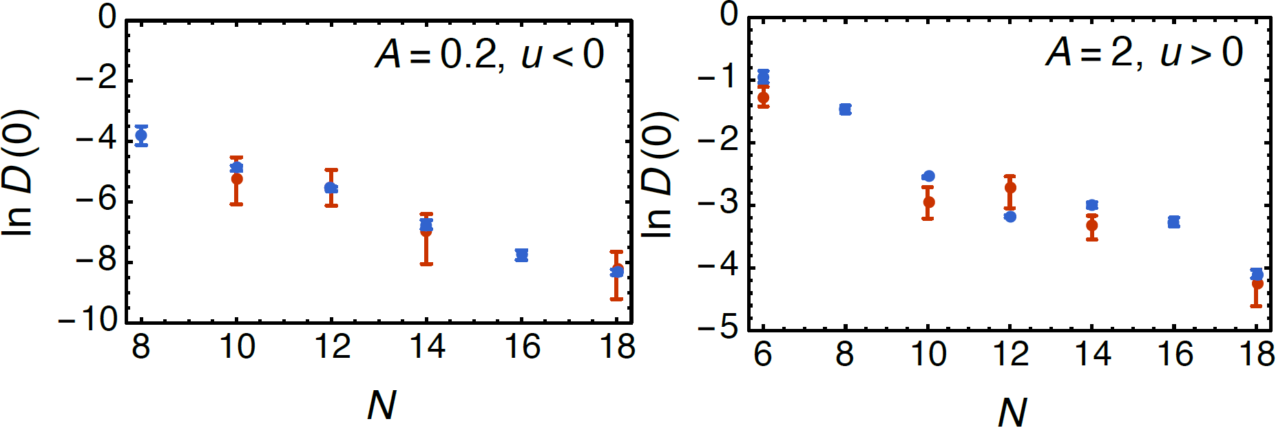
Figure 6: The logarithmic static correlation $\ln D(0)$ v.s. the fermion number $N$ for the case of $A=0.2$, $u<0$ (left), and $A=2$, $u>0$ (right). Neither case shows long range correlation of the bosonic field $b^{a}$. Both $D(\omega=0)$ (red) and $\lim_{\omega\to 0}D(\omega)$ (blue) are plotted in the figures.

For $A<1$ and $u<0$, the $u$ term flows to a stable fixed point $u^{\ast}\sim-(1-4/q)/C$. At this fixed point, since $u^{\ast}$ is an order-1 number, the fermion self-energy correction Fig. 3 is at the $M/N$ order, which vanishes in the large$-N$ limit for $A<1$. Thus the fermion scaling dimension remains the same as the SYK_q model: $\Delta_{f}=1/q$. But at this stable fixed point, the boson field $b^{a}\sim iC^{a}_{jk}\chi_{j}\chi_{k}$ acquires a correction, and has scaling dimension $\Delta_{b}=1-2/q$ in the large$-N$ limit. Starting with a SYK_q model with $q>4$, changing the sign of $u$ will drive a chaotic-nonchaotic transition with exponent $\nu=q/(q-4)$.

III.2 cases with $A>1$

For $A>1$, the RG equation is uncontrolled because the higher order terms in the beta function dominate in the large$-N$ limit. However, we can understand the model by taking the limit $M\rightarrow+\infty$ first. One intuitive way to think about this case is that according to the central limit theorem $\sum_{a=1}^{M}C^{a}_{ij}C^{a}_{kl}$ with $M\rightarrow+\infty$ follows the Gaussian distribution. So for either sign of $u$, Eq. 26 should behave the same as the $q=4$ SYK model. In order to explicitly demonstrate this statement, it is more convenient to use a different normalization of $C^{a}_{ij}$:

$$N^{(3+A)/2}\ \overline{C^{a}_{ij}C^{b}_{kl}}=J^{2}\delta_{ab}(\delta_{ik}\delta_{jl}-\delta_{il}\delta_{jk}).$$ (30)

We can perform the disorder average and integrating out $C^{a}_{ij}$, the leading order term in the large$-N$ limit is an eight-fermion interaction term $\sim\frac{u^{2}J^{4}}{N^{3}}\int\int d\tau d\tau^{\prime}(\chi_{i}(\tau)\chi_{i}(\tau^{\prime}))^{4}$, just like the disorder averaged $q=4$ SYK model, while all higher order $8n$-fermion interaction terms $\mathcal{S}^{(8n)}$ are suppressed $\sim\frac{(u^{2}J^{4})^{n}}{N^{3n+A(n-1)}}\left(\int\int d\tau d\tau^{\prime}(\chi_{i}(\tau)\chi_{i}(\tau^{\prime}))^{4}\right)^{n}$. Thus for $A>1$, the $u-$term actually behaves the same as the SYK model in the large$-N$ limit. This conclusion is consistent with the previous study of a similar generalization of the SYK model Danshita et al. (2016).

III.3 the $H^{\prime}$ term with $A=1$

$A=1$ is the critical situation, and the $H^{\prime}$ term itself (equivalent to taking $q=+\infty$ in Eq. 26) is already interesting enough when $A=1$. With the $H^{\prime}$ term only, we numerically solve the following coupled Schwinger-Dyson equations with the normalization from Eq. 30:

$$\tilde{G}_{f}(i\omega_{n})^{-1}=-i\omega_{n}-\tilde{\Sigma}_{f}(i\omega_{n}),\ \ \ \Sigma_{f}(\tau)=4\sqrt{\frac{M}{N}}u^{2}J^{2}G_{b}(\tau)G_{f}(\tau)$$ (31)

$$\tilde{G}_{b}(i\omega_{n})^{-1}=u-\tilde{\Sigma}_{b}(i\omega_{n}),\ \ \ \Sigma_{b}(\tau)=2\sqrt{\frac{N}{M}}u^{2}J^{2}G_{f}^{2}(\tau)$$ (32)

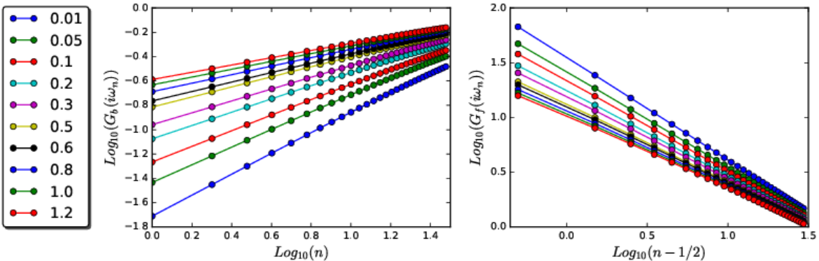
Figure 7: The numerical solution of Eq. 31,32, for $u=-1$, $J=1$, $\beta=300$ with different $M/N$, without assuming a conformal solution from the beginning. Both the boson and fermion Green’s functions have nice power-law scaling with the frequency, whose scaling dimensions depend on $M/N$.

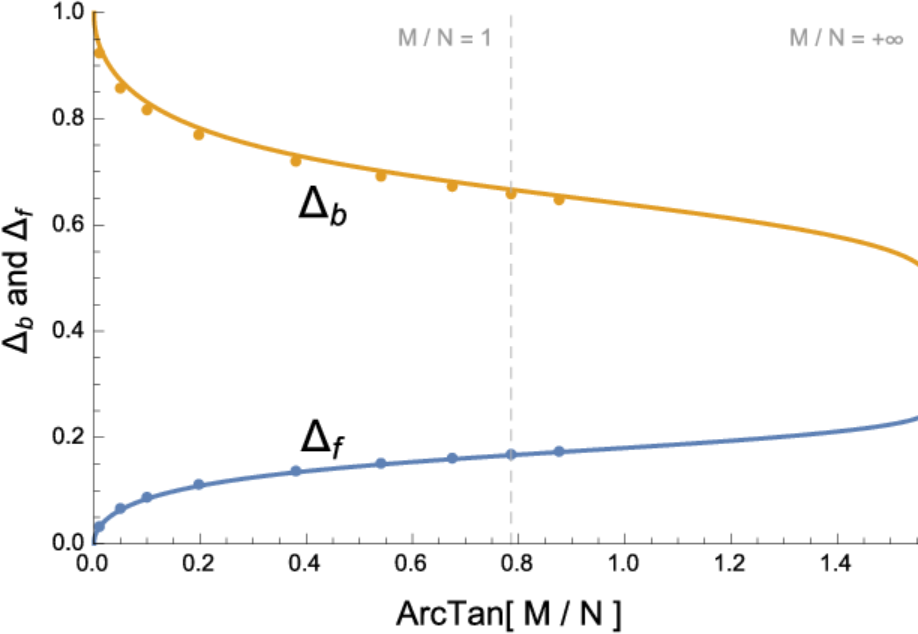
Figure 8: We numerically solve the Schwinger-Dyson equations (31-32) for $u=-1,J=1,\beta=300$ and fit the low frequency part as a power law. The scaling dimensions are continuous function of $M/N$, and for all the data points, the relation $2\Delta_{f}+\Delta_{b}=1$ is held. The solid curves plot the solution of the scaling dimensions based on Eq. 33. In particular, for $M/N=1$ (the dashed line), the scaling dimensions obtained from both the numerical and analytical solutions match with the prediction from the SUSY SYK model. Fu et al. (2016)

For the case with $A=1$ and $u<0$, the numerical solution of Eq. 31,32 generates well-converged power-law correlation functions for all $\alpha=M/N$, for both the fermion and boson fields (Fig. 7). And the scaling dimensions always satisfy $2\Delta_{f}+\Delta_{b}=1$.

Alternatively, by assuming that $G_{b}(\tau)\sim B/|\tau|^{2\Delta_{b}}$ and $G_{f}(\tau)\sim F\ \mathrm{sgn}(\tau)/|\tau|^{2\Delta_{f}}$ in the infrared limit, Eq. 31,32 reduce to the following equation for $\Delta_{b}$ for each ratio $M/N$:

$$2\frac{M}{N}\frac{\sin^{2}\left(\frac{\pi}{2}\Delta_{b}\right)}{\sin^{2}\left(\pi\Delta_{b}\right)}\frac{\Gamma(\Delta_{b})\Gamma(-\Delta_{b})}{\Gamma(2\Delta_{b})\Gamma(-2\Delta_{b})}\frac{2\Delta_{b}-1}{2\Delta_{b}}=-1.$$ (33)

$\Delta_{f}$ can be determined by $\Delta_{b}+2\Delta_{f}=1$. In particular, for $M/N=1$, our solution matches with the result of the SUSY SYK model Fu et al. (2016), where the model also has $M/N=1$ and $u<0$. The numerical solutions of Eq. 31,32 and analytical solution of Eq. 33 are both plotted in Fig. 8. With small $M/N$, $\Delta_{f}$ is approximately $\Delta_{f}\sim 1/\pi\sqrt{M/N}$.

IV Summary and Discussion

In this work we have demonstrated through various methods that the non-Fermi liquid fixed point of the SYK₄ model is instable against a class of marginally relevant four fermion perturbations, and these perturbations drive the system into a non-chaotic state with zero ground state entropy, and spontaneous time-reversal symmetry breaking. Because these perturbations are only marginally relevant, this effect occurs at exponentially low energy scale for a fixed strength of the perturbation. Spontaneous time-reversal symmetry breaking in experimental systems can be probed through Kerr rotation, which has been successfully applied to various condensed matter systems Kapitulnik et al. (2009); Spielman et al. (1990, 1992); Xia et al. (2006). Similar perturbations (with an opposite sign) can drive the SYK_q model with $q>4$ to a series of fixed points with continuously varying scaling dimensions.

So far we have ignored the replica index, for instance in Eq. 17. We will provide a self-consistent justification for this procedure. The usual argument for ignoring the replica index after disorder averaging the SYK interaction $J_{ijkl}$ is that, the replica off-diagonal terms are subleading in $1/N$ expansion Gu et al. (2016). Here we will investigate the replica index introduced after disorder averaging $C^{a}_{jk}$, and we only need to consider the case with $A\leq 1$, since as we have argued before, the case with $A>1$ is equivalent to the SYK₄ model.

Starting with the boson-fermion interaction term, $-iuC^{a}_{jk}b_{a}\chi_{j}\chi_{k}$, reinstating the replica index after disorder-average will lead to the following term

$$\sim-\frac{u^{2}J^{2}}{N^{2}}\sum_{\alpha,\beta}\int d\tau\int d\tau^{\prime}\sum_{a=1}^{M}b^{a}_{\alpha}(\tau)b^{a}_{\beta}(\tau^{\prime})\left(\chi^{\alpha}_{j}(\tau)\chi^{\beta}_{j}(\tau^{\prime})\right)^{2}.$$ (34)

In the phase where $b^{a}_{\alpha}$ does not condense (corresponds to $u<0$ in our case), the usual perturbation argument like Ref. Gu et al., 2016 will conclude that the replica off-diagonal terms will always make subleading contribution to the partition function compared with the diagonal terms. In the phase with $b^{a}$ condenses ($A<1$, $u>0$), the mean field solution tells us that $\sum_{a=1}^{M}\langle b^{a}_{\alpha}(\tau)b^{a}_{\beta}(\tau^{\prime})\rangle$ in Eq. 34 is at order of $N$. Then the perturbation argument will tell us when $u>0$ and $A<1$, the contribution from the replica off-diagonal terms is still subleading. Thus for all the main conclusions of this work, we can always make the replica diagonal assumption, and hence ignore the replica index.

The authors thank Wenbo Fu, Yingfei Gu, Xiao-Liang Qi, Subir Sachdev for very helpful discussions. Zhen Bi and Cenke Xu are supported by the David and Lucile Packard Foundation and NSF Grant No. DMR-1151208.

References

- Hertz (1976) J. A. Hertz, Phys. Rev. B 14, 1165 (1976), URL http://link.aps.org/doi/10.1103/PhysRevB.14.1165.
- Millis (1993) A. J. Millis, Phys. Rev. B 48, 7183 (1993), URL http://link.aps.org/doi/10.1103/PhysRevB.48.7183.
- Löhneysen et al. (2007) H. v. Löhneysen, A. Rosch, M. Vojta, and P. Wölfle, Rev. Mod. Phys. 79, 1015 (2007), URL http://link.aps.org/doi/10.1103/RevModPhys.79.1015.
- Lee (2009) S.-S. Lee, Phys. Rev. B 80, 165102 (2009), URL http://link.aps.org/doi/10.1103/PhysRevB.80.165102.
- Mross et al. (2010) D. F. Mross, J. McGreevy, H. Liu, and T. Senthil, Phys. Rev. B 82, 045121 (2010), URL http://link.aps.org/doi/10.1103/PhysRevB.82.045121.
- Metlitski and Sachdev (2010a) M. A. Metlitski and S. Sachdev, Phys. Rev. B 82, 075127 (2010a), URL http://link.aps.org/doi/10.1103/PhysRevB.82.075127.
- Metlitski and Sachdev (2010b) M. A. Metlitski and S. Sachdev, Phys. Rev. B 82, 075128 (2010b), URL http://link.aps.org/doi/10.1103/PhysRevB.82.075128.
- Dalidovich and Lee (2013) D. Dalidovich and S.-S. Lee, Phys. Rev. B 88, 245106 (2013), URL http://link.aps.org/doi/10.1103/PhysRevB.88.245106.
- Sachdev and Ye (1993) S. Sachdev and J. Ye, Physical Review Letters 70, 3339 (1993), eprint cond-mat/9212030.
- Kitaev (2015) A. Kitaev, A simple model of quantum holography, http://online.kitp.ucsb.edu/online/entangled15/kitaev/,http://online.kitp.ucsb.edu/online/entangled15/kitaev2/. (2015), Talks at KITP, April 7, 2015 and May 27, 2015.
- Maldacena and Stanford (2016) J. Maldacena and D. Stanford, Phys. Rev. D 94, 106002 (2016), eprint 1604.07818.
- Maldacena et al. (2016a) J. Maldacena, S. H. Shenker, and D. Stanford, Journal of High Energy Physics 8, 106 (2016a), eprint 1503.01409.
- Sachdev (2010) S. Sachdev, Phys. Rev. Lett. 105, 151602 (2010), URL http://link.aps.org/doi/10.1103/PhysRevLett.105.151602.
- Sachdev (2015) S. Sachdev, Physical Review X 5, 041025 (2015), eprint 1506.05111.
- Polchinski and Rosenhaus (2016) J. Polchinski and V. Rosenhaus, Journal of High Energy Physics 4, 1 (2016), eprint 1601.06768.
- Maldacena et al. (2016b) J. Maldacena, D. Stanford, and Z. Yang, ArXiv e-prints (2016b), eprint 1606.01857.
- Jensen (2016) K. Jensen, Phys. Rev. Lett. 117, 111601 (2016), URL http://link.aps.org/doi/10.1103/PhysRevLett.117.111601.
- Engelsöy et al. (2016) J. Engelsöy, T. G. Mertens, and H. Verlinde, Journal of High Energy Physics 2016, 139 (2016), ISSN 1029-8479, URL http://dx.doi.org/10.1007/JHEP07(2016)139.
- Georges et al. (2001) A. Georges, O. Parcollet, and S. Sachdev, Phys. Rev. B 63, 134406 (2001), eprint cond-mat/0009388.
- You et al. (2016) Y. Z. You, A. W. W. Ludwig, and C. Xu, arXiv:1602.06964 (2016).
- Fu and Sachdev (2016) W. Fu and S. Sachdev, Phys. Rev. B 94, 035135 (2016), eprint 1603.05246.
- Cotler et al. (2016) J. S. Cotler, G. Gur-Ari, M. Hanada, J. Polchinski, P. Saad, S. H. Shenker, D. Stanford, A. Streicher, and M. Tezuka, ArXiv e-prints (2016), eprint 1611.04650.
- Fu et al. (2016) W. Fu, D. Gaiotto, J. Maldacena, and S. Sachdev, ArXiv e-prints (2016), eprint 1610.08917.
- Gu et al. (2016) Y. Gu, X.-L. Qi, and D. Stanford, ArXiv e-prints (2016), eprint 1609.07832.
- Davison et al. (2016) R. A. Davison, W. Fu, A. Georges, Y. Gu, K. Jensen, and S. Sachdev, ArXiv e-prints (2016), eprint 1612.00849.
- Witten (2016) E. Witten, ArXiv e-prints (2016), eprint 1610.09758.
- Klebanov and Tarnopolsky (2016) I. R. Klebanov and G. Tarnopolsky, ArXiv e-prints (2016), eprint 1611.08915.
- Turiaci and Verlinde (2017) G. Turiaci and H. Verlinde, ArXiv e-prints (2017), eprint 1701.00528.
- Banerjee and Altman (2016) S. Banerjee and E. Altman, ArXiv e-prints (2016), eprint 1610.04619.
- Gross and Rosenhaus (2016) D. J. Gross and V. Rosenhaus, arXiv:1610.01569 (2016).
- García-García and Verbaarschot (2016) A. M. García-García and J. J. M. Verbaarschot, Phys. Rev. D 94, 126010 (2016), URL http://link.aps.org/doi/10.1103/PhysRevD.94.126010.
- Krishnan et al. (2016) C. Krishnan, S. Sanyal, and P. N. B. Subramanian, arXiv:1612.06330 (2016).
- Metlitski et al. (2015) M. A. Metlitski, D. F. Mross, S. Sachdev, and T. Senthil, Phys. Rev. B 91, 115111 (2015), URL http://link.aps.org/doi/10.1103/PhysRevB.91.115111.
- Kitaev (2009) A. Kitaev, AIP Conf. Proc 1134, 22 (2009).
- Schnyder et al. (2009) A. P. Schnyder, S. Ryu, A. Furusaki, and A. W. W. Ludwig, AIP Conf. Proc. 1134, 10 (2009).
- Ryu et al. (2010) S. Ryu, A. Schnyder, A. Furusaki, and A. Ludwig, New J. Phys. 12, 065010 (2010).
- Kosterlit and Thouless (1973) J. M. Kosterlit and D. J. Thouless, J. Phys. C: Solid State Phys 6, 1181 (1973).
- Danshita et al. (2016) I. Danshita, M. Hanada, and M. Tezuka, arXiv:1606.02454 (2016).
- Kapitulnik et al. (2009) A. Kapitulnik, J. Xia, E. Schemm, and A. Palevski, New Journal of Physics 11, 055060 (2009), URL http://stacks.iop.org/1367-2630/11/i=5/a=055060.
- Spielman et al. (1990) S. Spielman, K. Fesler, C. B. Eom, T. H. Geballe, M. M. Fejer, and A. Kapitulnik, Phys. Rev. Lett. 65, 123 (1990), URL https://link.aps.org/doi/10.1103/PhysRevLett.65.123.
- Spielman et al. (1992) S. Spielman, J. S. Dodge, L. W. Lombardo, C. B. Eom, M. M. Fejer, T. H. Geballe, and A. Kapitulnik, Phys. Rev. Lett. 68, 3472 (1992), URL https://link.aps.org/doi/10.1103/PhysRevLett.68.3472.
- Xia et al. (2006) J. Xia, Y. Maeno, P. T. Beyersdorf, M. M. Fejer, and A. Kapitulnik, Phys. Rev. Lett. 97, 167002 (2006), URL https://link.aps.org/doi/10.1103/PhysRevLett.97.167002.