Imaging Spectropolarimeter for Multi-application Solar Telescope at Udaipur Solar Observatory: Characterization of polarimeter and preliminary observations

1 Introduction

Solar activity is driven by spatio-temporal distribution of magnetic field (e.g. Solanki (2003), Borrero and Ichimoto (2011), Stix (2004)). Therefore, the precise measurements of the magnetic field in the solar atmosphere is of fundamental importance. The Zeeman effect (Zeeman, 1897) has been recognized as the most authentic tool for more than a century to derive the magnetic field of sunspots and pores in the photosphere (Stenflo, 2015, and references therein). With the advancement of instrumentation capabilities, one can now measure the Zeeman signals of a small-scale structure present in the photosphere as well as in the chromosphere (Trujillo Bueno, 2014; Wiegelmann, Petrie, and Riley, 2015). However, for the estimation of the weak field in the corona, the Zeeman effect becomes completely insensitive. Therefore, we rely on the Hanle effect (Hanle, 1924) for coronal magnetic field measurements. In special cases, both these effect can be combined to have magnetic field measurements in different atmospheric layers of the Sun (Lagg et al., 2015).

In the presence of magnetic field, light gets polarized and depolarized. The polarization of light is described in terms of the Stokes parameters I, Q, U, and V (Chandrasekhar, 1960; Born and Wolf, 1999) where I give the total intensity, Q and U represent the linear polarization and V represents the circular polarization. The spectropolarimeter consists of a filtergraph/spectrograph and a polarimeter, is employed to derive the solar vector magnetic fields by measuring Stokes I, Q, U, and V. Generally, two different techniques have been commonly used for spectral analysis: (1) imaging (filter) based (2) slit-based. For polarization analysis either single beam polarimeter or dual-beam polarimeter is employed. In imaging based spectropolarimetry, 2-D images are obtained in a sequence by tuning a narrow-band filter to different wavelengths along the spectral line profile of interest. Modern imaging spectropolarimeters employ either single or multiple Fabry-Perot (FP) etalon as narrow-band filters because of their high transmission and fast tuning capability. Few examples of the currently working imaging spectropolarimeters are: GREGOR Fabry-Perot instrument (GFPI; Denker et al. (2010)), KIS/IAA Visible Imaging Polarimeter (VIP; Beck et al. (2010)), CRisp Imaging Spectro-Polarimeter (CRISP, Scharmer et al. (2008)), the Gottingen spectropolarimeter (Bello González and Kneer, 2008), Interferometric BIdimensional Spectrometer (IBIS; Cavallini (2006)) and Imaging Vector Magnetograph (IVM; Mickey et al. (1996)). The Imaging Magnetograph eXperiment (IMaX; Martínez Pillet et al. (2011)) flown with the the Sunrise balloon mission (Barthol et al., 2011) is another example of imaging spectropolarimeter using a voltage tunable Lithium Niobate Fabry-Perot etalon. These instruments differ in the number of etalons and the optical configuration (telecentric or collimated). On the other hand, slit-based spectropolarimeter obtains the spectrum by scanning the required field-of-view (FOV) in sequence. Examples of slit-based spectropolarimeters are: Diffraction Limited Spectro-Polarimeter (DLSP; Sankarasubramanian et al. (2003)), the POlarimetric LIttrow Spectrograph (POLIS; Beck et al. (2005)), the Spectro-Polarimeter for Infrared and Optical Regions (SPINOR; Socas-Navarro et al. (2006)), and spectropolarimeter of the Solar Optical Telescope (SOT) onboard Hinode (Ichimoto et al. (2008), Tsuneta et al. (2008)). Based on the scientific requirement either of the above mentioned techniques are preferred. However, with the advances in the technology, both these techniques yield similar results.
In order to measure the vector magnetic field in the solar atmosphere, we have developed an imaging spectropolarimeter for Multi Application Solar Telescope (MAST) (Denis et al., 2008, 2010; Mathew, 2009) which is recently installed at the lake site of Udaipur Solar Observatory (USO). It is an off-axis Gregorian telescope with a 50 cm aperture. Along with adaptive optics system, the telescope is designed to provide near diffraction limited observations. One of the scientific objectives of MAST is to study the evolution of vector magnetic field in the solar atmosphere at different heights and its connection to various solar activities. Imaging spectropolarimeter for MAST consists of a narrow-band imager (Raja Bayanna et al., 2014) and a polarimeter which are used to measure the Stokes vector at two different wavelengths i.e. at 6173 Å and 8542 Å, corresponding to photospheric and chromospheric heights, respectively.
This paper has been arranged in the following manner. Section 2 describes the design of the polarimeter and the modulation scheme to measure the Stokes vector. The characterization of the liquid crystal variable retarders (LCVRs) with voltage and temperatures are discussed in Section 3. In Section 4 we explain the response matrix of the polarimeter derived using an experimental setup in the laboratory. Preliminary observations obtained with our instrument are presented in Section 5. Summary of the paper is provided in Section 6.

2 Polarimeter schematic and components

A polarimeter measures the polarization of the light by modulating the input polarization into measurable intensities. In general, the polarization analysis can be done in two ways (Del Toro Iniesta, 2003, and references therein): (a) Temporal polarization modulation/single beam polarimetry: Here, the different polarization measurements are obtained sequentially. The time gap between the measurements could introduce seeing related spurious signals in the difference image (Lites (1987); Leka and Rangarajan (2001)). This can be minimized either by compensating the atmospheric turbulence by adaptive optics or by implementing a very fast modulation scheme, wherein one modulation cycle is completed before atmospheric seeing changes completely, or by both. However, this imposes stringent requirements of the polarization modulator. (b) Spatial polarization modulation/Dual beam polarimetry (Lites, 1987): Here the orthogonal polarization states are separated by means of the polarizing beam splitter or displacer and both the beams are recorded simultaneously. This cancels out the fluctuations in the Stokes I to the other Stokes parameters caused due to atmospheric seeing (Martínez Pillet et al., 2011). Since both the beams are used for final computation of Stokes parameters, this method improves signal-noise-ratio (SNR) by a factor of $\sqrt{2}$ as compared to the single beam polarimetry. However, different optical paths for the measurements of two polarization states might introduce a systematic error; this puts a stringent requirement on the quality of the two optical paths in the experimental setup. It also requires a larger area of the detector to accommodate larger FOV.

Though the dual beam polarimetry is advantageous than the single beam polarimetry, we preferred to use single beam setup to perform the polarization analysis over a larger FOV. The fast modulation scheme with Liquid crystal variable retarders along with a matching fast camera readout, enable us to complete the modulation cycle before the seeing changes significantly. With suitable large format camera and a polarizing beam displacer, we plan to implement the dual beam spectropolarimetry with MAST at a later stage.

The main components of the MAST polarimeter are LCVRs for polarization modulation and Glan-Thompson polarizer as analyzer. Many of the recent polarization modulators also use liquid crystals, in which retardance (as in nematic liquid crystals) or fast axis (as in ferroelectric liquid crystals) can be changed by applying voltages (Heredero et al., 2007, and references therein). These modulators allow us to implement fast modulation schemes by avoiding mechanical motions and beam wobble as in the case of rotating retarders (Heredero et al., 2007). In MAST two sets of LCVRs along with a linear polarizer are used for obtaining the Stokes parameters. LCVRs for MAST polarimeter are custom made nematic liquid crystal devices with an aperture size of 80 mm, procured from Meadowlark Optics, USA. Figure 1 shows the schematic of MAST polarimeter. The fast axis of LCVR1 and LCVR2 are fixed at $0^{\circ}$ and $45^{\circ}$ with respect to the linear polarizer (LP), respectively. Light from the telescope enters through the LCVR1, passes through the LCVR2 and exits from the LP. Both LCVRs and the LP are mounted in rotating mounts to make the adjustment for the angles. The photograph of the installed system is shown in Figure 2. The temperature of the LCVRs is actively controlled using flexible heaters fixed on the holder; a temperature sensor in closed loop provides a thermal stability of $\pm$1${}^{\circ}C$.

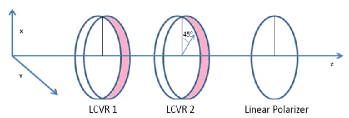
Figure 1.: Schematic layout of the polarimeter for MAST. The fast axis of LCVR1 and LCVR2 are kept at $0^{\circ}$ and $45^{\circ}$ with respect to the linear polarizer.

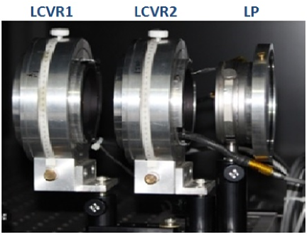
Figure 2.: Imaging polarimeter for MAST at USO. From left to right LCVR1, LCVR2 and linear polarizer. The LCVR1 and LCVR2 are kept at $0^{\circ}$ and $45^{\circ}$ with respect to the linear polarizer (LP), respectively.

The retardance of the LCVR can be changed by applying voltages. The modulation voltages for the LCVRs are supplied from a Meadowlark digital interface. The amplitude of the basic 2 KHz square waveform can be adjusted by an input DC voltage or counts provided from the software through a USB computer interface. Modulation voltages in the range of $0-10$ V with 16-bits accuracy can be applied to the LCVRs from this interface. C-programs have been written for the image acquisition in synchronization with the modulation voltages. The modulation scheme employed here is described in the following subsection.

2.1 Modulation scheme for the MAST polarimeter

As discussed in the previous section, the MAST polarimeter consists of two LCVRs and a linear polarizer. The Stokes vector of input light ($S_{in}$) at LCVR1 and the Stokes vector of output light at LP ($S_{out}$), are related using Mueller-matrix formalism by the following equation:

$$S_{out}=M_{P}M_{LC2}(\gamma,\theta_{2})M_{LC1}(\delta,\theta_{1})S_{in}=M_{S}S_{in}$$ (1)

where $M_{P}$, $M_{LC1}(\delta,\theta_{1})$, and $M_{LC2}(\gamma,\theta_{2})$ are the Mueller matrices of the linear polarizer, LCVR1 and LCVR2, respectively. The fast axis of LCVR1 and LCVR2 with respect to the transmission axis of the linear polarizer is represented by $\theta_{1}$ and $\theta_{2}$, respectively. The retardance of the LCVR1 and LCVR2 are given by $\delta$ and $\gamma$, respectively. $M_{S}$ is the resultant Mueller matrix of the polarimeter for a particular value of $\delta,\gamma,\theta_{1}$, and $\theta_{2}$.

Using the Mueller matrix of the retarder and polarizer in the Equation (1), intensity I, measured at CCD, can be expressed as a linear combination of all the input Stokes parameters as shown below.

$$I_{j}=S_{out}^{0}=1S_{in}^{0}+a_{j}S_{in}^{1}+b_{j}S_{in}^{2}+c_{j}S_{in}^{3},$$ (2)

where the parameters $[1,a_{j},b_{j},c_{j}]$ are the first row of $M_{S}$ which depend on $\theta_{1}$, $\theta_{2}$, $\delta$, and $\gamma$. Here j runs over the number of observations (from 1 to n). From Equation (2), we can measure n number of intensities for different combinations of retardances and fast axis orientations of both the LCVRs. However, it is always preferred to have a minimum number of intensity measurements to infer all the Stokes parameters (del Toro Iniesta and Collados, 2000). For vector polarimetry a minimum four measurements (n $\geq$ 4) are needed whereas longitudinal polarimetry can be done with two measurements (n $\geq$ 2) only. Therefore for n intensity measurements, a modulation scheme is fully characterized by a $(\textit{n}\times 4)$ modulation matrix O built from the n first rows of $M_{S}$,

$$I_{meas}=\textbf{O}S_{in}.$$ (3)

The Stokes vector is derived using the following Equation,

$$\textbf{S}_{in}=\textbf{O}^{-1}\textbf{I}_{meas}=\textbf{D}I_{meas}.$$ (4)

If n$=4$, then O is a $4\times 4$ matrix so its inverse will be unique. But, if n $=$ 6 then O is $6\times 4$ matrix, which is not a square matrix, and its inverse will not be unique. Hence, when D is not a square matrix, it is determined using the following Equation (del Toro Iniesta and Collados, 2000),

$$\textbf{D}=(\textbf{O}^{T}\textbf{O})^{-1}\textbf{O}^{T}.$$ (5)

The efficiency of the modulation scheme is defined as,

$$e_{i}=(\textit{n}\sum_{j=1}^{\textit{n}}\textbf{D}_{ij}^{2})^{-1/2},$$ (6)

where, $\textit{e}_{1}$, $\textit{e}_{2}$, $\textit{e}_{3}$, and $\textit{e}_{4}$ are the efficiencies for measuring the Stokes parameter I, Q, U, and V respectively.
For four measurement modulation scheme (n=4),

$$I_{meas}=\left[\begin{array}[]{c}I_{1}\\ I_{2}\\ I_{3}\\ I_{4}\end{array}\right]=\textbf{O}\left[\begin{array}[]{c}S_{in}^{0}\\ S_{in}^{1}\\ S_{in}^{2}\\ S_{in}^{3}\end{array}\right],$$ (7)

where O is the modulation matrix given as,

$$\textbf{O}=\begin{pmatrix}1&a_{1}&b_{1}&c_{1}\\ 1&a_{2}&b_{2}&c_{2}\\ 1&a_{3}&b_{3}&c_{3}\\ 1&a_{4}&b_{4}&c_{4}\end{pmatrix}.$$ (8)

For the polarimeter configuration shown in Figure 1 orientation of the fast axis of LCVR1 and LCVR2 is fixed at $\theta_{1}=0^{\circ}$, and $\theta_{2}=45^{\circ}$, respectively (Martinez Pillet et al., 2004). Using different combinations of retardances of LCVR1 and LCVR2, i.e., $\delta$ and $\gamma$, four and six measurement modulation schemes are implemented for vector polarimetry at MAST. The modulation schemes of four and six measurements are listed in Table 1 and 2.

Table 1.: Four measurement modulation scheme (Martinez Pillet et al., 2004) for vector polarimetry.

$\delta$	$\gamma$	Measured Intensity
(∘)	(∘)	$I_{meas}$
315.0	305.264	$I_{1}$$=$$I+Q/\sqrt{3}+U/\sqrt{3}+V/\sqrt{3}$
315.0	54.736	$I_{2}$$=$$I+Q/\sqrt{3}-U/\sqrt{3}-V/\sqrt{3}$
225.0	125.264	$I_{3}$$=$$I-Q/\sqrt{3}-U/\sqrt{3}+V/\sqrt{3}$
225.0	234.736	$I_{4}$$=$$I-Q/\sqrt{3}+U/\sqrt{3}-V/\sqrt{3}$

Table 2.: Six measurement modulation scheme (Tomczyk et al., 2010) for vector polarimetry.

$\delta$	$\gamma$	Measured Intensity
(∘)	(∘)	$I_{meas}$
180.0	360.0	$I_{1}=I+Q$
180.0	180.0	$I_{2}=I-Q$
090.0	090.0	$I_{3}=I+U$
090.0	270.0	$I_{4}=I-U$
180.0	090.0	$I_{5}=I+V$
180.0	270.0	$I_{6}=I-V$

The modulation matrix (O) for the four measurement modulation scheme is given by,

$$\textbf{O}=\begin{pmatrix}1&$0.57735$&$0.57735$&$0.57735$\\ 1&$0.57735$&$-0.57735$&$-0.57735$\\ 1&$-0.57735$&$-0.57735$&0.57735\\ 1&$-0.57735$&$0.57735$&$-0.57735$\end{pmatrix}.$$ (9)

For this modulation scheme, the maximum efficiencies are determined from Equations (5) and (6) as $\textit{e}_{1}=1$, $\textit{e}_{2}=0.57735$, $\textit{e}_{3}=0.57735$, and $\textit{e}_{4}=0.57735$.
Similarly, the modulation matrix for six measurement modulation scheme can be expressed as a $6\times 4$ matrix,

$$\textbf{O}=\begin{pmatrix}1&1&0&0\\ 1&$-1$&0&0\\ 1&0&1&0\\ 1&0&$-1$&0\\ 1&0&0&1\\ 1&0&0&$-1$\\ \end{pmatrix}.$$ (10)

For this modulation scheme, the maximum efficiencies are determined as $\textit{e}_{1}=1$, $\textit{e}_{2}=0.57735$, $\textit{e}_{3}=0.57735$, and $\textit{e}_{4}=0.57735$. These are the maximum efficiencies that an ideal polarimeter system can have (del Toro Iniesta and Collados, 2000).
Both the modulation schemes provide equal modulation efficiencies for the measurement of Q, U, and V (Del Toro Iniesta and Martínez Pillet, 2012). Either of these modulation schemes can be used for the measurement of all the Stokes parameters in vector polarimetry. Measurement of all the Stokes parameters is required to obtain the vector magnetic field, whereas the longitudinal magnetic field can be obtained from Stokes I and V only. The longitudinal measurement could be done by two intensity measurements. The modulation scheme for longitudinal polarimetry is listed in Table 3.

Table 3.: Modulation scheme for longitudinal polarimetry

$\delta$	$\gamma$	Measured Intensity
(∘)	(∘)	$I_{meas}$
360.0	90.0	$I_{1}=I-V$
360.0	270.0	$I_{2}=I+V$

The relation between the incoming Stokes vector and measured Stokes vector is given as (Beck et al., 2005),

$$S_{meas}=\textbf{X}.S_{in},$$ (11)

where X is the $4\times 4$ square matrix known as response matrix which includes all the processes for polarimetric measurement such as properties of optical components, modulation schemes and their demodulation (de Juan Ovelar et al., 2014; Beck et al., 2005). Furthermore, X can be expressed as

$$\textbf{X}=\textbf{D}\textbf{O}.$$ (12)

In the response matrix of an ideal polarimeter, the diagonal elements will be unity and the off-diagonal elements will be zero. However, in practice off-diagonal element of the response matrix will have non-zero values representing the cross-talk between the Stokes parameters introduced due to several reasons (de Juan Ovelar et al., 2014).

3 Characterization of the LCVRs

The retardance of the LCVRs can be tuned by applying voltages. The voltage dependence of retardance of LCVR is given by the following Equation (Saleh and Teich, 2007),

$$\delta=\frac{2\pi d}{\lambda}\left(\left(\frac{sin^{2}(\Theta)}{n_{o}^{2}}+\frac{cos^{2}(\Theta)}{n_{e}^{2}}\right)^{-\frac{1}{2}}-n_{e}\right),$$ (13)

where, $n_{o}$ and $n_{e}$ are the refractive indices of the ordinary and extraordinary beam and the equilibrium tilt angle $\Theta$ for liquid crystal molecules depends on the applied voltage, which is described by

$$\Theta =0,\hskip 5.69046pt\forall\hskip 5.69046ptV\leq V_{C}$$

$$=\frac{\pi}{2}-2\tan^{-1}\left(\exp\left(-\frac{V-V_{C}}{V_{0}}\right)\right),\hskip 5.69046pt\forall\hskip 5.69046ptV>V_{C},$$

where, $V$ is the applied voltage, $V_{C}$ is the critical voltage at which the tilting process begins, and $V_{0}$ is a constant.
The change in the retardance of LCVR due to temperature can be expressed by a semi-empirical formula (Li, Gauzia, and Wu, 2004; Capobianco et al., 2008),

$$\delta=\delta_{0}\,A=\delta_{0}\left(1-\frac{T}{T_{C}}\right)^{\alpha}$$ (14)

where $\delta_{0}$ is the retardance for A=1; A denotes an order parameter which describes the orientational order of nematic liquid crystal. For completely random and isotropic liquid crystals A=0, whereas for a perfectly aligned sample A=1 (Haller, 1975). For a typical liquid crystal sample, A is in the range of 0.3 to 0.8 and generally decreases with temperature (J. W. O-T., 1975; Shin-Tson Wu, 2001). In particular, a sharp drop of A to zero value is observed when the system undergoes a phase transition from the liquid crystal phase into the isotropic phase. Thus, $T_{C}$ is the nematic-isotropic transition temperature and $\alpha$ is critical exponent related to the phase transition. In order to use the LCVRs in the modulation scheme discussed in the previous Section, it is important to have the exact knowledge of retardance and its dependence on voltage and temperature.

3.1 Experimental setup and theory

Experimental setup for the characterization of LCVRs is shown in Figure 3. We have used a stabilized DC lamp as a white light source (S) along with a diffuser to get uniform intensity. A lens (C1) is placed in front of the pinhole to collimate the light. An interference filter (F1) is used to select the particular wavelength for which characterization of the LCVRs is carried out. The LCVR is placed in between two Glan-Thompson polarizing prisms (P1 & P2). Glan-Thompson polarizing prisms offers high extinction ratio (1$\times$$10^{-6}$) and high transmittance for a wavelength band between 3500-23000 Å (Hecht, 2001). Another lens (C2) is placed after the analyzer (P2) to image the beam onto a CCD camera to measure the intensity of output light. The incoming light is linearly polarized by the polarizer P1. After being retarded by the LCVR, whose fast axis is at 45^∘ the light is analyzed by the second polarizer P2. Polarizer P2 is mounted on a computer controlled rotation stage to measure the intensities at two different orientations.

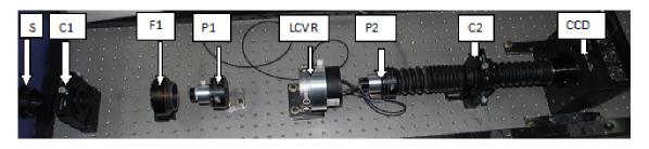
Figure 3.: Experimental setup for the calibration of LCVRs: In this setup, a light beam coming from a pinhole source is collimated using a lens C1. Then the collimating light passes through an interference filter (F1), linear polarizer (P1) and LCVR whose fast axis is kept at $45^{\circ}$ with respect to P1. Finally, light is imaged by imaging lens (C2) on CCD which is placed in the focal plane of the imaging lens after passing through analyzer P2.

The Stokes vector $S_{out}$ after P2 can be written as

$$\textbf{$S_{out}$}=M_{POL}M_{R}(\delta)\textbf{$S_{in}$},$$ (15)

where $S_{in}=[1100]^{T}$ represents the light linearly polarized by the polarizer P1. $M_{R}(\delta)$ and $M_{POL}$ are the Mueller matrix for the LCVR and the polarizer P2, respectively. $M_{R}(\delta)$ and $M_{POL}$ can be written as

$$M_{R}(\delta)=\begin{pmatrix}1&0&0&0\\ 0&cos^{2}2\phi+sin^{2}2\phi cos\delta&sin2\phi cos2\phi(1-cos\delta)&-sin2\phi sin\delta\\ 0&sin2\phi cos2\phi(1-cos\delta)&sin^{2}2\phi+cos^{2}2\phi cos\delta&cos2\phi sin\delta\\ 0&sin2\phi sin\delta&-cos2\phi sin\delta&cos\delta\end{pmatrix}.$$ (16)

$$M_{POL}(\theta)=\frac{1}{2}\begin{pmatrix}1&cos2\theta&sin2\theta&0\\ cos2\theta&cos^{2}2\theta&sin2\theta cos2\theta&0\\ sin2\theta&sin2\theta cos2\theta&sin^{2}{2}\theta&0\\ 0&0&0&0\end{pmatrix}.$$ (17)

where, $\phi$ is the orientation of the fast axis with respect to P1, $\delta$ is the retardance of LCVR due to the voltage applied, and $\theta$ is the orientation angle of P2 with respect to P1.
Substituting $M_{R}$, $M_{POL}$ and $S_{in}$ in Equation (15), the output intensity ($I_{out}$) measured by the CCD is

$$I_{out}=\frac{1}{2}\left[1+cos2\theta(cos^{2}2\phi+sin^{2}2\phi cos\delta)+sin2\theta sin2\phi cos2\phi(1-cos\delta)\right].$$ (18)

In our setup, we always keep $\phi$=$45^{\circ}$. Hence, Equation (18) becomes

$$I_{out}=\frac{1}{2}\left[1+cos2\theta cos\delta\right].$$ (19)

For $\theta=0^{\circ}$, where P2 is parallel to P1, output intensity is

$$I_{out}^{0}=\frac{1}{2}\left[1+cos\delta\right].$$ (20)

For $\theta=90^{\circ}$, where P2 is crossed to P1, the output intensity is

$$I_{out}^{90}=\frac{1}{2}\left[1-cos\delta\right].$$ (21)

Using Equations (20) and (21), retardance of LCVR can be obtained as

$$\delta=cos^{-1}\left(\frac{I_{out}^{0}-I_{out}^{90}}{I_{out}^{0}+I_{out}^{90}}\right).$$ (22)

Thus, by measuring the intensities $I_{out}$ for two different angles, $\theta=90^{\circ}$ and $\theta=0^{\circ}$, by rotating the polarizer P2, retardance $\delta$ of the LCVR can be estimated for different voltages. However, it requires prior knowledge of transmission axis of polarizers and the fast axis of LCVR. Hence, we determined the transmission axis of polarizers and the fast axis of LCVR using the same experimental setup before we carried out the characterization of LCVR.

Figure 4.: Variation of intensity with the rotation of polarizer P2 with respect to polarizer P1. The minimum intensity gives the angle at which both the polarizers are crossed to each other.

3.2 Determination of the crossed position of polarizers

In order to precisely align the axis of the polarizers P1 and P2, LCVR, shown in Figure 3, is removed from the optical path. By keeping polarizer P1 at a fixed position, polarizer P2 is rotated from $0^{\circ}$ to $180^{\circ}$ with respect to P1, with a step size of 1^∘ using a computer controlled rotation stage. For each angle, the intensity is measured using the CCD. The plot between the angle and the measured intensity is shown in Figure 4. Initially, when P1 and P2 are in parallel position the intensity is maximum. The intensity starts decreasing with the increase in the angle between them. At crossed position we get the minimum intensity which further starts increasing with the increase in the angle between P1 and P2. The above result satisfies the following equation

$$M_{P1}(\theta=0^{\circ}).M_{P2}(\theta=90^{\circ})=0.$$

3.3 Determination of the fast axis of LCVR

Knowing the crossed position of polarizers P1 and P2, we proceed to determine the fast axis of LCVR. For this purpose, polarizers P1 and P2 are kept in crossed position and LCVR is again placed between them. After that, output intensity is measured by rotating the LCVR. Figure 5 shows the plot between measured intensity and angle of the LCVR with respect to P1. The angle at which minimum intensity is observed is the angle at which fast axis of LCVR is parallel to P1. By knowing this angle, we rotate the fast axis of LCVR to 45^∘ with respect to P1 for further characterization of the LCVR. The above procedure can be easily understood by solving the following Mueller matrix Equation

$$M_{P1}(\theta=0^{\circ}).M_{LCVR}(\phi=0^{\circ},\delta).M_{P2}(\theta=90^{\circ})=0.$$

Figure 5.: Variation of intensity with the rotation of the fast axis of LCVR. The minimum intensity gives the position where the fast axis of LCVR is parallel with the polarizer P1.

  

                              

  

                              

Figure 6.: Calibration curves of the LCVR1 (top panels) and LCVR2 (bottom panels) at 6173 Å showing retardance as a function of voltage. Left (a and c) and right (b and d) panels show the voltages for the required retardance in vector and longitudinal modes, respectively. Vector mode will be used for the measurement of all the Stokes parameters and longitudinal mode will be used only for measuring Stokes parameters I and V.

  

                              

  

                              

Figure 7.: Calibration curves of the LCVR1 (top panels) and LCVR2 (bottom panels) at 8542 Å showing retardance as a function of voltage. Left (a and c) and right (b and d) panels show the voltages for the required retardance in vector and longitudinal modes, respectively. Vector mode will be used for the measurement of all the Stokes parameters and longitudinal mode will be used only for measuring Stokes parameters I and V.

3.4 LCVRs: Voltage versus retardance

After knowing the crossed position of polarizers and the fast axis of LCVRs, we characterize the dependence of voltage on the retardance of the LCVRs using the following procedure. Keeping the polarizers P1 and P2 in crossed position and the fast axis of LCVR at $45^{\circ}$ with respect to P1, we applied voltages from $0$ to $10$ V in steps of $0.05$ V to the LCVR. At each voltage five images were taken and computed the mean intensity to obtain $I_{out}^{90}$. Following the same procedure, $I_{out}^{0}$ as a function of voltage is obtained by rotating P2 such that P1 and P2 are in parallel position. In both the cases, the temperature of LCVR is kept constant at $28^{\circ}$C.

Table 4.: Obtained voltages for the required retardance at 6173 Å in the vector mode.

$\delta_{1}$	Voltage of LCVR1	$\delta_{2}$	Voltage of LCVR2
(∘)	(V)	(∘)	(V)
315.0	2.0977	305.264	2.2734
315.0	2.0977	054.736	5.0480
225.0	2.5984	125.264	3.6152
225.0	2.5984	234.736	2.6513

Table 5.: Obtained voltages for the required retardance at 6173 Å in the longitudinal mode.

$\delta_{1}$	Voltage of LCVR1	$\delta_{2}$	Voltage of LCVR2
(∘)	(V)	(∘)	(V)
360.0	1.8681	090.00	4.1608
360.0	1.8681	270.00	2.4539

With the measured $I_{out}^{0}$ and $I_{out}^{90}$ at each voltage, the retardance is calculated using Equation (22). The retardance of LCVRs (LCVR1 and LCVR2) with voltage for 6173 Å and 8542 Å are plotted and shown in Figure 6 and 7, respectively. The characteristics plots between retardance and voltage are used to estimate the voltages required in both the modulation schemes (vector and longitudinal). Figures 6 (a) and 6 (c) represent the corresponding voltages required for the retardance in vector mode modulation scheme (shown by circle on the characteristic curve) and Figures 6 (b) and 6 (d) represent the corresponding voltages required for the retardance in longitudinal mode modulation scheme, for LCVR1 and LCVR2 at wavelength 6173 Å, respectively.
Similarly, panels (a) and (c) of Figure 7 represent corresponding voltages required for the retardance in vector mode modulation scheme and panels (b) and (d) of Figure 7 represent corresponding voltages required for the retardance in longitudinal mode modulation scheme for LCVR1 and LCVR2 at wavelength 8542 Å, respectively.
The retardance and their corresponding voltages calibrated from Figures 6 and 7 are listed in Table $1-4$ for both the LCVRs according to their respective wavelengths. These values are used for the measurement of Stokes parameters with the polarimeter for MAST.

Table 6.: Obtained voltages for the required retardance at 8542 Å in the vector mode.

$\delta_{1}$	Voltage of LCVR1	$\delta_{2}$	Voltage of LCVR2
(∘)	$(V)$	(∘)	$(V)$
315.0	2.1139	305.264	1.8982
315.0	2.1139	054.736	4.3853
225.0	2.6038	125.264	3.1203
225.0	2.6038	234.736	2.2618

Table 7.: Obtained voltages for the required retardance at 8542 Å in the longitudinal mode.

$\delta_{1}$	Voltage of LCVR1	$\delta_{2}$	Voltage of LCVR2
(∘)	$(V)$	(∘)	$(V)$
360.0	1.8749	090.00	3.6031
360.0	1.8749	270.00	2.0736

Figure 8.: Variation of the retardance with the applied voltage of LCVR for four different temperatures. It is evident that as temperature increases the retardance of the LCVR decreases.

3.5 LCVRs: Temperature versus retardance

As evident from Equation (14) that the temperature also influences retardance of LCVRs, we have characterized voltage dependence of retardance of a LCVR at four different temperatures, i.e., $28^{\circ}$C, $30^{\circ}$C, $35^{\circ}$C, and $40^{\circ}$C. Figure 8 shows a change in retardance of LCVR with the voltage at different temperatures. As evident from Figure 8, retardance of the LCVR decreases as their temperature increases. The effect of temperature on the retardance of the LCVR can be clearly seen in Figure 9. It shows that the LCVR is more sensitive to the temperature when it is operated at low voltages $(0-4V)$ (Li, Gauzia, and Wu, 2004; Capobianco et al., 2008). Maximum change in the retardance with the temperature of $\sim-1.5^{\circ}$/^∘C is observed at $2.0$ V. At present the LCVRs are kept in a temperature enclosures provided by the vendor. Temperature stability of the enclosure is $\pm 1^{\circ}$C.
For precise polarimetric measurements, it is important to know the change in response matrix due to the fluctuations in the temperature enclosure. As mentioned above, $\pm 1.0^{\circ}$C variation in temperature causes a maximum change in retardance of $-$1.5^∘. Incorporating the change in retardance, the new response matrix can be written as,

$$\textbf{X \textprime}=\begin{pmatrix}0.99983&0.00017&0.01309&-0.01309\\ 0.00017&0.99983&-0.01309&0.01309\\ -0.01309&0.01309&0.99983&0.00017\\ 0.01309&-0.01309&0.00017&0.99983\end{pmatrix}.$$ (23)

Thus, the error in the measurement of response matrix is,

$$\Delta\textbf{X}=\textbf{X}-\textbf{X\textprime}=\begin{pmatrix}0.00017&-0.00017&-0.01309&0.01309\\ -0.00017&0.00017&0.01309&-0.01309\\ 0.01309&-0.01309&0.00017&-0.00017\\ -0.01309&0.01309&-0.00017&0.00017\end{pmatrix},$$

where X is unity matrix. The matrix element (3, 2), (4, 2), (4, 3) of $X\textprime$ shows the cross-talk among the Stokes parameters Q, U, and V. In this case, the cross-talk from Q to U and Q to V is same and equal to $1.3\times 10^{-2}$ and U to V cross-talk is $1.7\times 10^{-4}$. As the expected polarimetric accuracy is poorer, we calculated the change in polarimetric accuracy for different value of temperature accuracy. Table 8 summarises the calculations. For a temperature variation of $\pm 0.25^{\circ}$C (which can be obtained by optimizing the temperature control system), causes an error in retardance of $\pm 0.38^{\circ}$ (as shown in Table 8), the cross-talk will be in the order of $10^{-3}$ which would be acceptable for our scientific studies. Therefore a temperature control system which can maintain the temperature of LCVRs within $\pm 0.25^{\circ}$C will be constructed and used for the measurements of the Stokes parameters.

Table 8.: Polarimetric cross-talk due to change in the temperature stability ($\delta T$) of the temperature enclosure.

$\delta T$	Q $\rightarrow$ U	Q$\rightarrow$ V	$U\rightarrow V$
(∘C)	cross-talk	cross-talk	cross-talk
1.00	$1.3\times 10^{-2}$	$1.3\times 10^{-2}$	$1.7\times 10^{-4}$
0.50	$6.5\times 10^{-3}$	$6.5\times 10^{-3}$	$4.25\times 10^{-5}$
0.25	$3.2\times 10^{-3}$	$3,2\times 10^{-3}$	$1.04\times 10^{-5}$

  

Figure 9.: Left: Change in retardance with the change in temperature for different voltages. Right: retardance derivative with respect to the temperature as a function of voltage which shows that LCVR is insensitive to temperature for higher voltages.

3.6 LCVRs: Change in the orientation of the fast axis with the voltage

It is presumed that the angular position of the LCVR fast axis is independent of the voltage, only the retardation changes according to the voltage. But in practice, it is observed that the position of the fast axis also changes with the voltage (Terrier, Charbois, and Devlaminck, 2010). In order to see the effect of voltage on the orientation of the fast axis of LCVR, we performed the following experiment. Two polarizers P1 and P2 are placed in a collimated beam keeping P1 at a reference position and intensity is measured by rotating P2 from $0^{\circ}-180^{\circ}$. After knowing the crossed position of the polarizers P1 and P2, LCVR is placed between P1 and P2. The orientation of LCVR is adjusted such that the fast axis of LCVR becomes parallel to polarizer P1 (Figure 10). In this configuration, rotating the P2 gives exactly the same kind of intensity variation as in the case of crossed linear polarizers. Without changing the orientation of the LCVR, we apply different voltages (between 0-10 V) to LCVR and measured the intensity variation by rotating P2. We observed that (Figure 10, left) the intensity variation is sinusoidal again, and the sinusoid pattern for different voltages is shifted with respect to the reference sinusoid (no LCVR). The difference between the reference position (no LCVR or without voltage) and the actual position for different voltages is measured and plotted against the applied voltage for LCVR1 (see Figure 10, right).

  

Figure 10.: Left panel shows the variation of intensity with the change in angular position of polarizer P2 with reference to polarizer P1 for different voltages applied to the LCVR. The right panel shows the shift in the position of the fast axis with the voltage applied to the LCVR in which reference is taken as no LCVR position.

As shown in Figure 10 (right), the maximum shift obtained in the orientation of the fast axis of LCVR is $8^{\circ}$ at $2.5$ V. Thus, it is important to know the change in response matrix due to the shift in the orientation of fast axis. The new response matrix due to the change in the orientation of the fast axis ($8^{\circ}$) is,

$$\textbf{X\textprime}=\begin{pmatrix}0.99454&0.03327&0.05467&-0.08248\\ 0.03327&0.99454&0.05467&-0.08248\\ 0.30782&-0.20404&0.92874&-0.03252\\ 0.30782&-0.20404&-0.03252&0.92874\end{pmatrix}.$$ (24)

The error in the measurement of modulation matrix is,

$$\Delta\textbf{X}=\textbf{X}-\textbf{X\textprime}=\begin{pmatrix}0.00546&-0.03327&-0.05467&0.08248\\ -0.03327&0.00546&-0.05467&0.08248\\ -0.30782&0.20404&0.07126&0.03252\\ -0.30782&0.20404&0.03252&0.07126\end{pmatrix},$$

where X is unity matrix. The matrix element (3, 2), (4, 2), (4, 3) of $X\textprime$ shows the cross talk among the Stokes parameters Q, U, and V. In this case the cross-talk from Q to U and Q to V is same and equal to $2.0\times 10^{-1}$ and U to V cross-talk is $3.2\times 10^{-2}$.

As evident from the above analysis the cross-talk in the Stokes measurement resulting from the drift in the LCVR fast axis while applying voltages is considerably large and need to be taken care of. The theoretical modulation matrix O (Equation (9)) is modified by including the drift in the fast axis for corresponding voltages. This modified modulation matrix is used for the demodulation of the observed Stokes profiles (Terrier, Charbois, and Devlaminck, 2010).

4 Experimental determination of response matrix of the polarimeter

As discussed in Section 2.1, the relation between the incoming Stokes vector and measured Stokes vector can be written as

$$S_{meas}=\textbf{X}.S_{in},$$ (25)

where X is the $4\times 4$ element response matrix. The response matrix of the polarimeter can be determined experimentally from the measured Stokes parameters of the known input polarizations generated by calibration unit consisting of a zero order quarter wave plate (QWP) and a linear polarizer. We have computed the response matrix of the polarimeter in the laboratory using experimental setup shown in Figure 11 for both the wavelengths (6173 Å and 8542 Å).

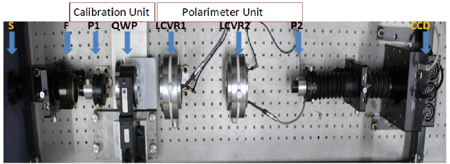
Figure 11.: Experimental setup for the calibration of response matrix for MAST polarimeter. In this setup, a light beam is collimated using lens L1 and then collimating light passes through an interference filter (F), calibration unit consists of a linear polarizer (P1) and a zero order quarter wave plate (QWP), and polarimeter consists of two LCVRs (LCVR1 and LCVR2) and a linear polarizer (P2). Finally, image is formed by imaging lens on CCD which is placed in the focal plane of the imaging lens.

For the response matrix calibration, the calibration unit (CU) is placed in the beam before the polarimeter module as shown in the Figure 8. The orientation of the axes has been determined with an accuracy of $\textpm 1^{\circ}$ for the linear polarizer, and $\textpm 0.5^{\circ}$ for the QWP of CU which has been fixed in a computer controlled rotating mount. To determine X of the polarimeter, 80 known polarization states are created by rotating QWP from $0^{\circ}-160^{\circ}$ with a step size of $2^{\circ}$ and measured by the polarimeter using four intensity measurement modulation scheme (Table 1) and six measurement modulation scheme (Table 2) as discussed in Section 2.1. We have computed the response matrix of the polarimeter using both the schemes. Here, we discuss the response matrix calibration using four measurement modulation scheme in detail.

  

                              

  

                              

Figure 12.: Plots of input Stokes parameters and demodulated Stokes parameters calculated at each position angles of QWP of CU for 6173 Å wavelength.

For the configuration shown in Figure 11, the input Stokes vector can be written as,

  

                              

  

                              

Figure 13.: Plots of input Stokes parameters and demodulated Stokes parameters calculated at each position angles of QWP of CU for 8542 Å wavelength.

$$S_{in}=M_{QWP}(\theta_{r},\delta).M_{P1}(\theta_{p}).[1000]^{T},$$

where, $\theta_{r}$ and $\theta_{p}$ are the orientation of the retarder and polarizer of the CU relative to the reference axis and $\delta$ is the retardance of QWP. In our case, we fixed $\theta_{p}$ at $0^{\circ}$, then the input Stokes parameters for different retarder orientation is given by,

$$\left.\begin{aligned} I=1,\\ Q=cos^{2}(2\theta)+sin^{2}(2\theta).cos(\delta),\\ U=sin(2\theta).cos(2\theta).(1-cos(\delta)),\\ V=-sin(2\theta).sin(\delta).\end{aligned}\right\}$$ (26)

For n orientations of CU retarder, polarimeter response matrix is calibrated from the measurements after rearranging the Stokes vector into n$\times$4 matrices by a solution of the linear problem,

$$S_{meas}=X.S_{in},$$

Multiplying by $S_{in}^{T}$ from the right in above Equation

$$S_{meas}.S_{in}^{T}=X.S_{in}.S_{in}^{T}=X.D,$$

where

$$D=S_{in}.S_{in}^{T}.$$

Therefore, the final expression for response matrix is

$$X=S_{meas}.S_{in}^{T}.D^{-1}.$$ (27)

Hence, response matrix for 6173 Å is determined from the above Equation using input and measured Stokes vector is given by

$$X_{4}^{6173}=\begin{pmatrix}1.0000&-0.0507&-0.0054&-0.0595\\ -0.0090&0.8946&-0.1618&-0.0369\\ -0.0447&-0.0639&0.8314&0.0734\\ -0.0474&-0.1494&0.0647&0.9665\\ \end{pmatrix}$$ (28)

Thus, the real incoming Stokes vector ${\mathbfit S_{in}}$ can be calculated from the observed Stokes vector and measured response matrix as follows,

$${\mathbfit S_{in}}=X^{-1}.S_{meas}.$$

The input and the demodulated Stokes parameters at each CU retarder orientation are shown in Figure 12.
Similarly, we have determined the response matrix of the polarimeter at 8542 Å wavelength and given by,

$$X_{4}^{8542}=\begin{pmatrix}1.0000&0.0006&0.0349&-0.0965\\ -0.0009&0.8931&-0.1053&0.0041\\ -0.0135&-0.0616&0.9073&-0.1809\\ 0.0873&0.0452&0.1948&0.9115\\ \end{pmatrix},$$ (29)

and plots for the input and demodulated input Stokes parameters are shown in Figure 13.

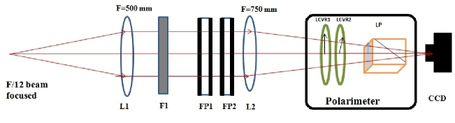
Figure 14.: Schematic diagram of the imaging polarimeter for MAST. In this setup a F/12 beam from the telescope is collimated using the lens L1. The collimating beam passes through narrow-band imager consists of two Fabry-Perot etalons (FP1 and FP2) and prefilter F1. Polarimeter consist of two LCVR and a Glan-Thompson polarizer is kept in between the CCD and imaging lens (L2) in the converging beam. The F-number of the converging beam is 18.

4.1 Response matrix for six measurement modulation scheme

Similarly, we have also computed X when Stokes parameters were obtained by six measurement modulation scheme and the other procedures were same as discussed above. The response matrix of the polarimeter for 6173 Å is,

$$X_{6}^{6173}=\begin{pmatrix}1.0000&-0.0084&0.0153&-0.0016\\ 0.0009&0.9493&0.0265&0.1462\\ -0.0171&0.0254&0.9573&0.9491\\ 0.0043&-0.1829&-0.0808&0.9491\\ \end{pmatrix}.$$ (30)

Similarly, the response matrix of the polarimeter for 8542 Å is,

$$X_{6}^{8542}=\begin{pmatrix}1.0000&0.0062&-0.0177&0.0044\\ -0.0056&0.9251&0.0665&0.1308\\ -0.0652&0.0396&0.9454&0.0791\\ 0.0344&-0.1379&-0.1509&0.9176\\ \end{pmatrix}.$$ (31)

5 Preliminary observations of Stokes profiles

Preliminary observations were obtained using the imaging spectropolarimeter for MAST, consisting of a narrow-band imager and a polarimeter. The narrow-band imager is designed around two z-cut $LiNbO_{3}$ Fabry-Perot etalons placed in tandem to provide a better spectral resolution. The wavelength characterization of the components of the narrow band imager is described in a previous paper (Raja Bayanna et al., 2014). The integration and test results of the imager obtained with MAST will be presented in a separate paper (Mathew et al., (in preparation)). The full-width at half maximum (FWHM) of the FP combination is $\sim$95 mÅ at 6173 Å with an effective free-spectral range (FSR) of 6 Å. A blocking filter of 2.5 Å is introduced to restrict the FP channel of the desired wavelength. For the Ca II 8542 Å line we use only one etalon, with 175 mÅ FWHM. As explained earlier, polarimeter consists of a two LCVRs and a linear polarizer (Glan-Thompson polarizer).

The optical setup of the spectropolarimeter is shown in Figure 14. F$\#$12 beam from the telescope and its re-imaging optics is collimated using a lens (L1) of focal length 500 mm. The FPs are placed in this collimated beam in order to reduce the wavelength shift produced by the finite angle of incidence arising from the FOV. Collimated output through the FPs is imaged using a lens (L2) of focal length 750 mm, which forms a plate scale of $0.145^{\prime\prime}$pixel^-1 at the CCD plane. The polarimeter is placed in this converging beam after the lens L2, to accommodate smaller Glan-Thompson polarizer. The acceptance angles of the LCVRs are large enough to work with resultant F$\#$18 beam. Since the z-cut etalons with a small angle of incidence produce negligible polarization effects, we have not separately considered the effect of the etalons in polarization measurements. The fast axes of the first and second LCVRs are kept at $0^{\circ}$ and $45^{\circ}$ with respect to the polarization axis of the linear polarizer as described in section 2. The temperatures of the LCVRs are kept at $28^{\circ}C$.

For the present set of observations, we are modulating polarization first and wavelength later to minimize the seeing influence. The response time of LCVRs (for the change of one polarization state to other) is 22 ms. Change in wavelength position requires 100 ms and 200 ms for a spectral sampling of 15 mÅ, and 30 mÅ, respectively as the tuning speed of the FPs is nearly 1000 Vs^-1.

We capture 20 images for each polarizaton state to bulid-up the signal. Overall time taken for one modulation cycle (i.e. for obtaining IQUV at one wavelength poistion) is around 8 seconds considering an exposure time of 60 ms (at 6173 Å). Depending on the number of wavelength position the time cadance of the vector magnetogram varies; for e.g., the cadance varies from 40 seconds to 216 seconds for 5 to 27 wavelength positions, respectively. The number of wavelength points which determine the time cadance can be selected as required by the scientific objectives. A cadance of more than a minute is sufficent enough to study the evolution of active regions and energy build-up due to the foot point motions (Wiegelmann and Sakurai, 2012, and references therein). Magnetograms (by tuning the filter to a single wavelength position) can be obtained in 10 seconds cadance, which could be used for studying the magnetic field evolution of small scale moving magnetic features seen around the sunspot (Ma et al., 2015, and references therein). A six wavelength step scan, which takes around 50 seconds can reproduce the line profile as seen in SDO/HMI, suitable for the vector magnetic field retrieval , as long as the horizontal speed of the moving feature is below 3 kms^-1.

For the initial tests, we have scanned the spectral profile of 6173 Å line with a step of 15 mÅ and 30 mÅ, for a total of 27 and 20 positions, respectively in longitudinal and vector modes. The number of wavelength positions could be considerably reduced by an optimization after inverting the profiles, which will be carried out after further analysis. We obtained observations in longitudinal and vector modes described in Section 2.1.

  

                                     

  

                              

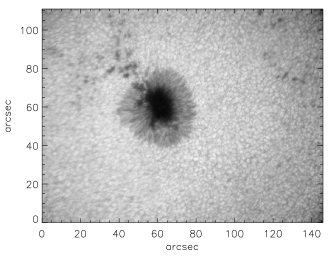
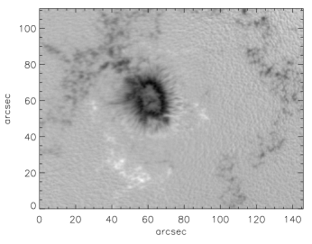
Figure 15.: LOS mode of observations of the active region NOAA AR 12436 observed on 24th October 2015 between 4:00 UT and 5:30 UT using MAST polarimeter. In the first row, the left Figure shows one of the mean intensity images whereas the right Figure is for the corresponding mean Stokes I profiles. The Stokes I profile is deduced separately for the magnetic (solid line) and for the non-magnetic (dashed lines) regions whereas in the second row, left Figure displays the mean Stokes V image for a wavelength position at $+75$ mÅ from line center and right plot indicates the mean Stokes V profile for both the magnetic and non-magnetic regions. Because of the limitation of the voltage tuning of both the etalons in tandem, line profile shifted more toward blue side.

5.1 Longitudinal mode

The observations described in this section were obtained for a sunspot in the active region NOAA AR 12436 taken on 24th October 2015 between 4:00 UT and 5:30 UT, when the seeing was moderate. The active region was slightly away from the disk center located at N09 and W20. FP etalons of the narrow-band imager were sequentially tuned to 27 positions on the 6173Å line, with 15 mÅ wavelength spacing. A pair of two images in left- and right- circular polarizations (LCP & RCP) was obtained by applying appropriate voltages (listed in Table 5) to the LCVR 1 and 2. For these measurements, the voltage of the LCVR1 is changed alternately, whereas the LCVR2 is kept constant to provide a retardance of 1$\lambda$. For each wavelength position, 20 pairs of LCP and RCP images were obtained with an exposure time of 65 ms to increase the signal to noise ratio (SNR). Figure 16 shows the results of the above observation. The top left Figure shows one of the mean intensity image whereas the right Figure is for the corresponding mean Stokes I profiles. The mean Stokes I profile is deduced separately for both the magnetic (solid line, where the V signal is more than $10^{-3}$) and for the non-magnetic (dashed line) regions. The broadening of the profile due to the magnetic field is evident in these plots. The bottom left Figure displays the mean Stokes V image for a wavelength position at $+75$ mÅ from line center whereas the right plot indicates the mean Stokes V profile for both the magnetic and non-magnetic regions.

5.2 Comparison of Stokes V images from SDO/HMI and USO/MAST

We also carried out a comparison of our results with the magnetograms availed from Helioseismic Magnetic Imager (HMI) instrument (Scherrer et al., 2012; Schou et al., 2012) onboard the Solar Dynamics Observatory (SDO) (Pesnell, Thompson, and Chamberlin, 2012). For comparison, the images from MAST and HMI were taken at around the same time (04:42 UT on 24th October 2015). The comparison was possible as the spectral line used by both the instruments is same, even though the spectral resolution of each instrument differs. SDO/HMI images are available for both the continuum and the line-of-sight (LOS) magnetic field, and also for the Stokes I, Q, U and V parameters as for right, left, circular and linear polarization images. For our present comparison, we constrained only to SDO/HMI LOS magnetograms and Stokes V images, since our polarization measurements need further instrumental polarization corrections. Even though the stokes V profiles could also get contaminated by the instrumental polarization, for a preliminary comparison the Stokes V images are suitable as the cross-talk from the linear polarization mostly introduce only a bias.
The images obtained from the SDO/HMI is resized, and the USO/MAST image is registered with respect to SDO/HMI image. The right and left images in the top panel of Figure 17 shows the cropped continuum images taken with SDO/HMI and USO/MAST instruments, respectively. The images are cropped in such a way that it include the sunspot and a part of the nearby area. The middle panel show the Stokes V images of SDO/HMI (left) and USO/MAST polarimeter (right), respectively for a selected wavelength position $+75$ mÅ (from the line center). It is evident from Figures that most of the magnetic features in the Stokes V map of SDO/HMI matches well with the Stokes V map of USO/MAST polarimeter. The advantage of the space-based observation is clearly visible in the SDO/HMI images as evident from the low background features.

Unlike SDO/HMI observations, the USO/MAST images are affected by the atmospheric seeing during the image acquisition which results in a considerable I$\rightarrow$V cross-talk (Del Toro Iniesta, 2003; Lites, 1987) thus a higher background noise. This I$\rightarrow$V cross-talk is evident from the granulation pattern in Stokes V images of USO/MAST.

The bottom Figures are for the Stokes V signal obtained at a wavelength position $+75$ mÅ (from the line center) plotted against the SDO/HMI LOS magnetic field strength. The plot shown in the left panel is for the USO/MAST Stokes V whereas the right is for the SDO/HMI Stokes V at a close by wavelength position against the SDO/HMI LOS magnetic field strength. The region shown with the red contain points mostly from the umbra, where the linearity between the Stokes V amplitude and the magnetic field strength doesn’t hold. As it is evident in Figure 16, other than the scatter which could be partly due to the seeing related I$\rightarrow$V cross-talk, the trend matches closely.

We also found a factor of around 2 in the Stokes V signal between the SDO/HMI and the USO/MAST images. This can be explained by the influence of finite width of the narrow band filter in scanning the line profile and the difference in the overall instrumental profiles used in the HMI and MAST imager. The finite width of the filter results in a convolution of the spectral line profile, which introduces an apparant increase in the width and decrease in the depth of the line profile. This effectively reduces the amplitude of the Stokes V signal. In order to check this we have computed, synthetic line profiles using M-E inversion code, taking realistic solar atmospheric parameters. Convolution of the Stokes V parameter with the filter profile of 95 mÅ FWHM shows a reduction in the peak of Stokes V amplitude by a similar factor, i.e., 2. This effect can be taken care while inverting the Stokes profiles; i.e., convolution of the synthetic profile with filter profile is carried out before fitting that with observed Stokes profiles. Other than the above differences, the overall comparison between the SDO/HMI and the USO/MAST Stokes V measurements provide the confidence in our measurements.

  

                                     

  

  

                              

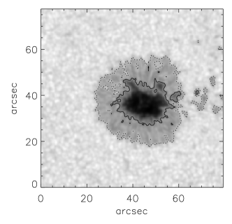
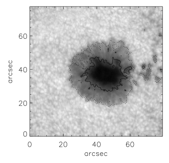
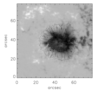
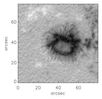
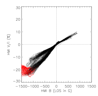
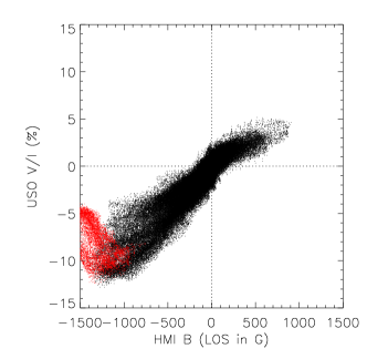
Figure 16.: Top row: Stokes I image taken by SDO/HMI (left) and USO/MAST (right); Middle row: Stokes V image at wavelength position $+75$ mÅ from line center taken by SDO/HMI (left) and USO/MAST (right); bottom row: scatter plot made between Stokes V of SDO/HMI and longitudinal magnetic field of SDO/HMI (left) and scatter plot made between Stokes V of USO/MAST and longitudinal magnetic field of SDO/HMI (right).

5.3 Vector mode

By operating the imaging polarimeter in vector mode, we have carried out observations on $19^{th}$ December 2015. The active region NOAA AR12470 (N15, W07) was observed during the period 06:00 UT and 07:30 UT. Four images were obtained sequentially by applying appropriate voltages (listed in Table 4) to the LCVRs. From the observed intensity images Stokes, I, Q, U and V images were computed for each wavelength position. Similar to the longitudinal mode the images in vector mode acquired by scanning the line profile with 15 mÅ spacing and at 27 wavelength positions. Figure 17 shows the images, top left and right panels shows the Stokes I, and Q, the bottom left and right panels show the U and V images, respectively. The Stokes U, Q, and V images are shown for a wavelength position at $+75$ mÅ from line center on the line profile. The bottom panel shows respective Stokes profiles for the single point marked by a star in the Stokes I image. A thorough analysis and demodulation of the linear polarization measurement requires the knowledge of the instrumental polarization. For this purpose, we are currently introducing a large (50 cm) sheet linear polarizer which can be rotated, in front of the primary mirror. This will enable us to characterize the telescope polarization before extracting the Stokes information from these measurements.

  

                              

  

                              

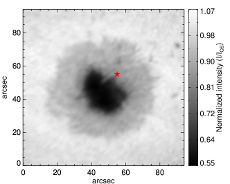
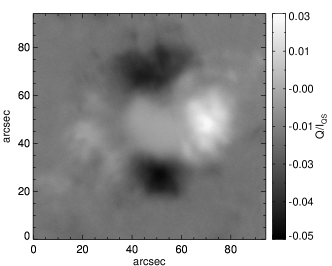
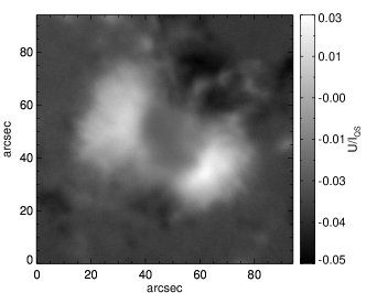
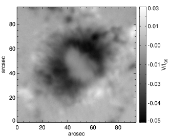
Figure 17.: Stokes images obtained using vector mode of operation for NOAA AR 12470 at 6173 Å are shown here. Top panels show Stokes I (left), Q (right). Bottom panels show Stokes U (left) and V (right).

Figure 18.: Profiles of Stokes parameters I, Q, U, and V at a point in the penumbra of NOAA AR 12470 corresponding to the star mark in Figure 17.

5.4 Observations on 16 April, 2016

As evident in the Stokes I profile in the top panel of Figure 15, the starting point for the wavelength scanning has a limited coverage in the blue wing side of the Fe I 6173 Å line profile. This was due to the limited tuning range of the Fabry-Perot filters, which was restricted due to the maximum voltage which could be applied to the etalons, and the operating temperatures of the etalons. As it is important to cover the entire wavelength range in order to obtain the continuum intensity at both sides of the line profile, we have carried out a re-tuning of the etalons to optimally cover the continuum at both the sides. Since the maximum allowed voltage which could be applied to the etalon is restricted, the re-tuning was done by changing the operating temperature. The re-tuning allowed us to start the line profile scan from a wavelength point further blue in the continuum. The following example of the Stokes V scan was carried after the re-tuning of the filters. These observations were taken on $16^{th}$ April 2016. Here the sunspot in the active region NOAA AR 12529 (N10, W38) was observed with the polarimeter. The observations were obtained between 07:00 UT and 07:30 UT. During data acquisition, the seeing was again moderate. Unlike the previous observations, instead of 27 wavelength positions, we increased the wavelength spacing to 30 mÅ which resulted in around 20 spectral positions on 6173 Å line for the wavelength scan. Figure 19 shows the images for the wavelength position $+75$ mÅ from the line center and the corresponding mean Stokes V profile (right) for the entire FOV. In this case, the wavelength scan started well in the blue continuum, and the Stokes V signal also covers enough continuum wavelength points.

  

                              

  

                              

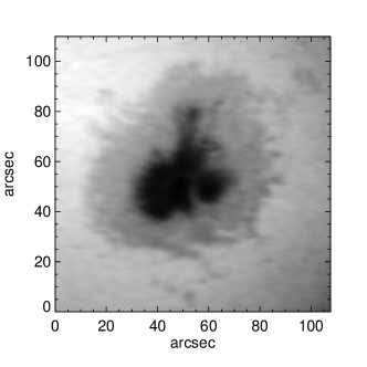
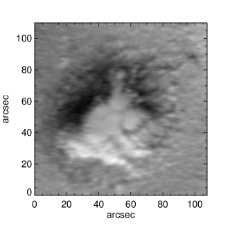
Figure 19.: Stokes I and V observations of the active region NOAA AR 12529 in the spectral line 6173 Å. Top Row: Mean intensity (Stokes I) image (left) and its mean intensity profile (right). Bottom Row: Mean Stokes V image (left) and its mean profile (right).

5.5 Stokes V measurement in CaII 8542 Å line

In this section, we report the circular polarization measurements obtained in the chromospheric CaII 8542 Å line. The measurements were carried out with the second pair of LCVRs specifically procured for this wavelength. The imager is tuned to the blue wing $-150$ mÅ from the line center. The LCVR is sequentially switched between voltages corresponding to the modulation voltages for the left and right circular polarizations. A pair of 100 images were obtained for this measurement with an exposure time of 120 ms for each image. In Figure 20, left image shows one of the selected I+V images from these observations, whereas the right panel shows the mean V image at the above wavelength point. A clear Stokes V signal is present in the difference image (Figure 20, right), the seeing variations and the long exposure times produce artifacts, which will definitely reduce by the ongoing adaptive optics installation. In the above observations, the images were taken only at one wavelength position, but the filter can be tuned to a considerable part of the CaII 8542 Å line profile, which will be done in the future observations. The linear polarization measurement is also planned for this line.

  

                                     

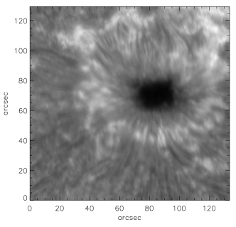
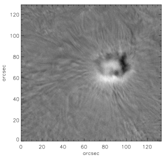
Figure 20.: Chromospheric observations in LOS mode of the active region NOAA AR 12546 (S07, E19) observed on $18^{th}$ May, 2016 between 08:30 UT and 08:36 UT using MAST polarimeter. Images of I+V (left) and mean Stokes parameter V (right) at a wavelength position $-150$ mÅ from the line center.

6 Summary

The imaging spectropolarimeter for MAST has been developed for obtaining the magnetic field information of the Sun in the spectral lines 6173 Å and 8542 Å, which are formed in photosphere and chromosphere, respectively. The spectropolarimeter includes an FP-based narrow-band filter, and a polarimeter consists of a pair of nematic LCVRs and a linear polarizer. In this paper, we have presented the characterization of the LCVRs, its retardance as a function of voltage and temperature.Response matrix of the polarimeter is obtained using an experimental setup. We have also discussed the implementation of four and six measurement schemes that are normally employed in obtaining the spectropolarimetric observations. Using the information obtained from the characterization of LCVRs, we have obtained preliminary observations in Fe I 6173 Å. For the testing purpose, these observations are acquired by scanning the line profile of Fe I 6173 Å at 27 wavelength positions with a sample of 15 mÅ. We plan to minimize the number of wavelength positions to $8-12$ to improve the cadence of the observations. As HMI also provides the similar observations, we compared the Stokes I and V observations from MAST with that of SDO/HMI. Qualitatively, both the observations are in good agreement with each other, considering the fact that MAST observations are seeing limited.

In order to obtain the vector magnetic fields of the active region, Stokes Q, and U along with Stokes I, and V are also obtained. However, we have not derived the magnetic fields from these observations as it requires information regarding instrument induced polarization. In this regard, it is important to note that MAST is a nine mirror system with two off-axis parabolic mirrors and 7 plane oblique mirrors. We have planned to obtain the instrument induced polarization both theoretically (Anche et al., 2015; Sen and Kakati, 1997) and experimentally (Selbing, 2010). In this paper, we have also presented the Stokes I and V observations of an active region in Ca II 8542 Å, which is formed in the chromosphere.

7 Acknowledgement

We sincerely thank the referee for valuable comments, which helped us to improve the content in the manuscript. The HMI data used here are courtesy of NASA/SDO and the HMI science team. We thank the HMI science team for making available the processed data of $I-V$ (LCP) and $I+V$ (RCP) for our comparative study. We also acknowledge the work of Mukesh M Sardava of USO in the design and fabrication of the mount for LCVRs and polarizers.

References

- Anche et al. (2015) Anche, R.M., Anupama, G.C., Reddy, K., Sen, A., Sankarasubramanian, K., Ramaprakash, A.N., Sengupta, S., Skidmore, W., Atwood, J., Tirupathi, S., Pandey, S.B.: 2015, Analytical modelling of Thirty Meter Telescope optics polarization. In: International Conference on Optics and Photonics 2015, Proc. SPIE 9654, 965408. DOI. ADS.
- Barthol et al. (2011) Barthol, P., Gandorfer, A., Solanki, S.K., Schüssler, M., Chares, B., Curdt, W., Deutsch, W., Feller, A., Germerott, D., Grauf, B., Heerlein, K., Hirzberger, J., Kolleck, M., Meller, R., Müller, R., Riethmüller, T.L., Tomasch, G., Knölker, M., Lites, B.W., Card, G., Elmore, D., Fox, J., Lecinski, A., Nelson, P., Summers, R., Watt, A., Martínez Pillet, V., Bonet, J.A., Schmidt, W., Berkefeld, T., Title, A.M., Domingo, V., Gasent Blesa, J.L., Del Toro Iniesta, J.C., López Jiménez, A., Álvarez-Herrero, A., Sabau-Graziati, L., Widani, C., Haberler, P., Härtel, K., Kampf, D., Levin, T., Pérez Grande, I., Sanz-Andrés, A., Schmidt, E.: 2011, The Sunrise Mission. Sol. Phys. 268, 1. DOI. ADS.
- Beck et al. (2005) Beck, C., Schmidt, W., Kentischer, T., Elmore, D.: 2005, Polarimetric Littrow Spectrograph - instrument calibration and first measurements. A&A 437, 1159. DOI. ADS.
- Beck et al. (2010) Beck, C., Bellot Rubio, L.R., Kentischer, T.J., Tritschler, A., Del Toro Iniesta, J.C.: 2010, Two-dimensional solar spectropolarimetry with the KIS/IAA Visible Imaging Polarimeter. A&A 520, A115. DOI. ADS.
- Bello González and Kneer (2008) Bello González, N., Kneer, F.: 2008, Narrow-band full Stokes polarimetry of small structures on the Sun with speckle methods. A&A 480, 265. DOI. ADS.
- Born and Wolf (1999) Born, M., Wolf, E.: 1999, Principles of optics, 7th edn. Cambridge University Press, ???.
- Borrero and Ichimoto (2011) Borrero, J.M., Ichimoto, K.: 2011, Magnetic Structure of Sunspots. Living Reviews in Solar Physics 8, 4. DOI. ADS.
- Capobianco et al. (2008) Capobianco, G., Crudelini, F., Zangrilli, L., Buscemi, C., Fineschi, S.: 2008, E-KPol Temperature Calibration. ADS.
- Cavallini (2006) Cavallini, F.: 2006, IBIS: A New Post-Focus Instrument for Solar Imaging Spectroscopy. Sol. Phys. 236, 415. DOI. ADS.
- Chandrasekhar (1960) Chandrasekhar, S.: 1960, Radiative transfer. ADS.
- de Juan Ovelar et al. (2014) de Juan Ovelar, M., Snik, F., Keller, C.U., Venema, L.: 2014, Instrumental polarisation at the Nasmyth focus of the E-ELT. A&A 562, A8. DOI. ADS.
- Del Toro Iniesta (2003) Del Toro Iniesta, J.C.: 2003, Introduction to Spectropolarimetry, 244. ADS.
- del Toro Iniesta and Collados (2000) del Toro Iniesta, J.C., Collados, M.: 2000, Optimum Modulation and Demodulation Matrices for Solar Polarimetry. Applied Optics 39, 1637. DOI. ADS.
- Del Toro Iniesta and Martínez Pillet (2012) Del Toro Iniesta, J.C., Martínez Pillet, V.: 2012, Assessing the Behavior of Modern Solar Magnetographs and Spectropolarimeters. ApJS 201, 22. DOI. ADS.
- Denis et al. (2008) Denis, S., Coucke, P., Gabriel, E., Delrez, C., Venkatakrishnan, P.: 2008, Optomechanical and thermal design of the Multi-Application Solar Telescope for USO. In: Ground-based and Airborne Telescopes II, Proc. SPIE 7012, 701235. DOI. ADS.
- Denis et al. (2010) Denis, S., Coucke, P., Gabriel, E., Delrez, C., Venkatakrishnan, P.: 2010, Multi-Application Solar Telescope: assembly, integration, and testing. In: Ground-based and Airborne Telescopes III, Proc. SPIE 7733, 773335. DOI. ADS.
- Denker et al. (2010) Denker, C., Balthasar, H., Hofmann, A., Bello González, N., Volkmer, R.: 2010, The GREGOR Fabry-Perot interferometer: a new instrument for high-resolution solar observations. In: Society of Photo-Optical Instrumentation Engineers (SPIE) Conference Series, Society of Photo-Optical Instrumentation Engineers (SPIE) Conference Series 7735, 6. DOI. ADS.
- Haller (1975) Haller, I.: 1975, Thermodynamic and static properties of liquid crystals. Progress in Solid State Chemistry 10, 103 . DOI. http://www.sciencedirect.com/science/article/pii/0079678675900084.
- Hanle (1924) Hanle, W.: 1924, Über magnetische Beeinflussung der Polarisation der Resonanzfluoreszenz. Zeitschrift fur Physik 30, 93. DOI. ADS.
- Hecht (2001) Hecht, E.: 2001, Optics 4th edition. ADS.
- Heredero et al. (2007) Heredero, R.L., Uribe-Patarroyo, N., Belenguer, T., Ramos, G., Sánchez, A., Reina, M., Martínez Pillet, V., Álvarez-Herrero, A.: 2007, Liquid-crystal variable retarders for aerospace polarimetry applications. Applied Optics 46, 689. DOI. ADS.
- Ichimoto et al. (2008) Ichimoto, K., Lites, B., Elmore, D., Suematsu, Y., Tsuneta, S., Katsukawa, Y., Shimizu, T., Shine, R., Tarbell, T., Title, A., Kiyohara, J., Shinoda, K., Card, G., Lecinski, A., Streander, K., Nakagiri, M., Miyashita, M., Noguchi, M., Hoffmann, C., Cruz, T.: 2008, Polarization Calibration of the Solar Optical Telescope onboard Hinode. Sol. Phys. 249, 233. DOI. ADS.
- J. W. O-T. (1975) J. W. O-T.: 1975, The Physics of Liquid Crystals . by P.G. de Gennes, Clarendon Press, Oxford, 1974. Journal of Molecular Structure 29, 190. DOI. ADS.
- Lagg et al. (2015) Lagg, A., Lites, B., Harvey, J., Gosain, S., Centeno, R.: 2015, Measurements of Photospheric and Chromospheric Magnetic Fields. ArXiv e-prints. ADS.
- Leka and Rangarajan (2001) Leka, K.D., Rangarajan, K.E.: 2001, Effects of ‘Seeing’ on Vector Magnetograph Measurements. Sol. Phys. 203, 239. DOI. ADS.
- Li, Gauzia, and Wu (2004) Li, J., Gauzia, S., Wu, S.-T.: 2004, High temperature-gradient refractive index liquid crystals. Optics Express 12, 2002. DOI. ADS.
- Lites (1987) Lites, B.W.: 1987, Rotating waveplates as polarization modulators for Stokes polarimetry of the sun - Evaluation of seeing-induced crosstalk errors. Applied Optics 26, 3838. DOI. ADS.
- Ma et al. (2015) Ma, L., Zhou, W., Zhou, G., Zhang, J.: 2015, The evolution of arch filament systems and moving magnetic features around a sunspot. A&A 583, A110. DOI. ADS.
- Martinez Pillet et al. (2004) Martinez Pillet, V., Bonet, J.A., Collados, M.V., Jochum, L., Mathew, S., Medina Trujillo, J.L., Ruiz Cobo, B., del Toro Iniesta, J.C., Lopez Jimenez, A.C., Castillo Lorenzo, J., Herranz, M., Jeronimo, J.M., Mellado, P., Morales, R., Rodriguez, J., Alvarez-Herrero, A., Belenguer, T., Heredero, R.L., Menendez, M., Ramos, G., Reina, M., Pastor, C., Sanchez, A., Villanueva, J., Domingo, V., Gasent, J.L., Rodriguez, P.: 2004, The imaging magnetograph eXperiment for the SUNRISE balloon Antarctica project. In: Mather, J.C. (ed.) Optical, Infrared, and Millimeter Space Telescopes, Society of Photo-Optical Instrumentation Engineers (SPIE) Conference Series 5487, 1152. DOI. ADS.
- Martínez Pillet et al. (2011) Martínez Pillet, V., Del Toro Iniesta, J.C., Álvarez-Herrero, A., Domingo, V., Bonet, J.A., González Fernández, L., López Jiménez, A., Pastor, C., Gasent Blesa, J.L., Mellado, P., Piqueras, J., Aparicio, B., Balaguer, M., Ballesteros, E., Belenguer, T., Bellot Rubio, L.R., Berkefeld, T., Collados, M., Deutsch, W., Feller, A., Girela, F., Grauf, B., Heredero, R.L., Herranz, M., Jerónimo, J.M., Laguna, H., Meller, R., Menéndez, M., Morales, R., Orozco Suárez, D., Ramos, G., Reina, M., Ramos, J.L., Rodríguez, P., Sánchez, A., Uribe-Patarroyo, N., Barthol, P., Gandorfer, A., Knoelker, M., Schmidt, W., Solanki, S.K., Vargas Domínguez, S.: 2011, The Imaging Magnetograph eXperiment (IMaX) for the Sunrise Balloon-Borne Solar Observatory. Sol. Phys. 268, 57. DOI. ADS.
- Mathew (2009) Mathew, S.K.: 2009, A New 0.5m Telescope (MAST) for Solar Imaging and Polarimetry. In: Berdyugina, S.V., Nagendra, K.N., Ramelli, R. (eds.) Solar Polarization 5: In Honor of Jan Stenflo, Astronomical Society of the Pacific Conference Series 405, 461. ADS.
- Mickey et al. (1996) Mickey, D.L., Canfield, R.C., Labonte, B.J., Leka, K.D., Waterson, M.F., Weber, H.M.: 1996, The Imaging Vector Magnetograph at Haleakala. Sol. Phys. 168, 229. DOI. ADS.
- Pesnell, Thompson, and Chamberlin (2012) Pesnell, W.D., Thompson, B.J., Chamberlin, P.C.: 2012, The Solar Dynamics Observatory (SDO). Sol. Phys. 275, 3. DOI. ADS.
- Raja Bayanna et al. (2014) Raja Bayanna, A., Mathew, S.K., Venkatakrishnan, P., Srivastava, N.: 2014, Narrow-Band Imaging System for the Multi-application Solar Telescope at Udaipur Solar Observatory: Characterization of Lithium Niobate Etalons. Sol. Phys. 289, 4007. DOI. ADS.
- Saleh and Teich (2007) Saleh, B.E.A., Teich, M.C.: 2007, Fundamentals of photonics. JOHN WILEY & SONS, INC. Chap. 18. 978-0471358329.
- Sankarasubramanian et al. (2003) Sankarasubramanian, K., Elmore, D.F., Lites, B.W., Sigwarth, M., Rimmele, T.R., Hegwer, S.L., Gregory, S., Streander, K.V., Wilkins, L.M., Richards, K., Berst, C.: 2003, Diffraction limited spectro-polarimeter - Phase I. In: Fineschi, S. (ed.) Polarimetry in Astronomy, Society of Photo-Optical Instrumentation Engineers (SPIE) Conference Series 4843, 414. DOI. ADS.
- Scharmer et al. (2008) Scharmer, G.B., Narayan, G., Hillberg, T., de la Cruz Rodríguez, J., Löfdahl, M.G., Kiselman, D., Sütterlin, P., van Noort, M., Lagg, A.: 2008, CRISP Spectropolarimetric Imaging of Penumbral Fine Structure. ApJ 689, L69. DOI. ADS.
- Scherrer et al. (2012) Scherrer, P.H., Schou, J., Bush, R.I., Kosovichev, A.G., Bogart, R.S., Hoeksema, J.T., Liu, Y., Duvall, T.L., Zhao, J., Title, A.M., Schrijver, C.J., Tarbell, T.D., Tomczyk, S.: 2012, The Helioseismic and Magnetic Imager (HMI) Investigation for the Solar Dynamics Observatory (SDO). Sol. Phys. 275, 207. DOI. ADS.
- Schou et al. (2012) Schou, J., Scherrer, P.H., Bush, R.I., Wachter, R., Couvidat, S., Rabello-Soares, M.C., Bogart, R.S., Hoeksema, J.T., Liu, Y., Duvall, T.L., Akin, D.J., Allard, B.A., Miles, J.W., Rairden, R., Shine, R.A., Tarbell, T.D., Title, A.M., Wolfson, C.J., Elmore, D.F., Norton, A.A., Tomczyk, S.: 2012, Design and Ground Calibration of the Helioseismic and Magnetic Imager (HMI) Instrument on the Solar Dynamics Observatory (SDO). Sol. Phys. 275, 229. DOI. ADS.
- Selbing (2010) Selbing, J.: 2010, SST polarization model and polarimeter calibration.
- Sen and Kakati (1997) Sen, A.K., Kakati, M.: 1997, Instrumental polarization caused by telescope optics during wide field imaging. A&AS 126. DOI. ADS.
- Shin-Tson Wu (2001) Shin-Tson Wu, D.-K.Y.: 2001, Reflective Liquid Crystal Displays, John Wiley and Sons, ???.
- Socas-Navarro et al. (2006) Socas-Navarro, H., Elmore, D., Pietarila, A., Darnell, A., Lites, B.W., Tomczyk, S., Hegwer, S.: 2006, Spinor: Visible and Infrared Spectro-Polarimetry at the National Solar Observatory. Sol. Phys. 235, 55. DOI. ADS.
- Solanki (2003) Solanki, S.K.: 2003, Sunspots: An overview. A&A Rev. 11, 153. DOI. ADS.
- Stenflo (2015) Stenflo, J.O.: 2015, History of Solar Magnetic Fields Since George Ellery Hale. Space Sci. Rev.. DOI. ADS.
- Stix (2004) Stix, M.: 2004, The sun, 2nd edn. Springer-verlag Gmbh, ???.
- Terrier, Charbois, and Devlaminck (2010) Terrier, P., Charbois, J.M., Devlaminck, V.: 2010, Fast-axis orientation dependence on driving voltage for a Stokes polarimeter based on concrete liquid-crystal variable retarders. Applied Optics 49, 4278. DOI. ADS.
- Tomczyk et al. (2010) Tomczyk, S., Casini, R., de Wijn, A.G., Nelson, P.G.: 2010, Wavelength-diverse polarization modulators for Stokes polarimetry. Applied Optics 49, 3580. DOI. ADS.
- Trujillo Bueno (2014) Trujillo Bueno, J.: 2014, Polarized Radiation Observables for Probing the Magnetism of the Outer Solar Atmosphere. In: Nagendra, K.N., Stenflo, J.O., Qu, Q., Samooprna, M. (eds.) Solar Polarization 7, Astronomical Society of the Pacific Conference Series 489, 137. ADS.
- Tsuneta et al. (2008) Tsuneta, S., Ichimoto, K., Katsukawa, Y., Nagata, S., Otsubo, M., Shimizu, T., Suematsu, Y., Nakagiri, M., Noguchi, M., Tarbell, T., Title, A., Shine, R., Rosenberg, W., Hoffmann, C., Jurcevich, B., Kushner, G., Levay, M., Lites, B., Elmore, D., Matsushita, T., Kawaguchi, N., Saito, H., Mikami, I., Hill, L.D., Owens, J.K.: 2008, The Solar Optical Telescope for the Hinode Mission: An Overview. Sol. Phys. 249, 167. DOI. ADS.
- Wiegelmann and Sakurai (2012) Wiegelmann, T., Sakurai, T.: 2012, Solar force-free magnetic fields. Living Reviews in Solar Physics 9(5). DOI. http://www.livingreviews.org/lrsp-2012-5.
- Wiegelmann, Petrie, and Riley (2015) Wiegelmann, T., Petrie, G.J.D., Riley, P.: 2015, Coronal Magnetic Field Models. Space Sci. Rev.. DOI. ADS.
- Zeeman (1897) Zeeman, P.: 1897, On the Influence of Magnetism on the Nature of the Light Emitted by a Substance. ApJ 5, 332. DOI. ADS.