SparseStep: Approximating the Counting Norm for Sparse Regularization

Abstract

The SparseStep algorithm is presented for the estimation of a sparse parameter vector in the linear regression problem. The algorithm works by adding an approximation of the exact counting norm as a constraint on the model parameters and iteratively strengthening this approximation to arrive at a sparse solution. Theoretical analysis of the penalty function shows that the estimator yields unbiased estimates of the parameter vector. An iterative majorization algorithm is derived which has a straightforward implementation reminiscent of ridge regression. In addition, the SparseStep algorithm is compared with similar methods through a rigorous simulation study which shows it often outperforms existing methods in both model fit and prediction accuracy.
Keywords: Sparse Regression, Feature Selection, Iterative Majorization

1 Introduction

In many modeling problems it is desirable to restrict the number of nonzero elements in the parameter vector to reduce the model complexity. Achieving this so-called sparsity in the model parameters for the regression problem is known to be NP-hard (Natarajan, 1995). Many alternatives have been presented in the literature which approximate the true sparse solution by applying shrinkage to the parameter vector, such as for instance the lasso estimator (Tibshirani, 1996). However, this shrinkage can underestimate the true effect of explanatory variables on the model outcome. Here, an algorithm is presented which creates sparse model estimates but does not apply shrinkage to the parameter estimates. This feature is obtained by approximating the exact counting norm and making this approximation increasingly more accurate.

Traditional methods for solving the exact sparse linear regression problem include best subset selection, forward and backward stepwise regression, and forward stagewise regression. These approaches may not always be feasible for problems with a large number of predictors and may display a high degree of variance with out-of-sample predictions (Hastie et al., 2009). Alternatively, penalized least-squares methods add a regularization term to the regression problem, to curb variability through shrinkage or induce sparsity, or both. Of the many more recent approaches to this problem, the most well-known are perhaps the SCAD penalty (Fan and Li, 2001) and the MC+ penalty (Zhang, 2010). In both of these approaches, a penalty is added such that the overall size of the model parameters can be controlled.

Figure 1 shows an illustration of the different penalty functions discussed above. Note that all penalty functions are symmetric around zero, including the SparseStep penalty introduced below. It can be seen that the shapes of the SCAD and MC+ penalties closely resemble each other. The different shapes of the penalty function for the SCAD and MC+ penalty are due to the parameter $a$, which can be optimized over for a given dataset. In contrast, the different shapes of the SparseStep penalty show subsequent approximations of the exact $\ell_{0}$ penalty, as described below.

This paper is organized as follows. In Section 2 the theory behind the SparseStep penalty is introduced and analyzed. Section 3 derives the SparseStep algorithm using the Iterative Majorization technique and describes the implementation of the algorithm. Experiments comparing SparseStep with existing methods are described extensively in the following section. Section 5 concludes.

(a) Ridge & Lasso

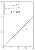
(b) SCAD

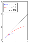
(c) MC+

(d) SparseStep

Figure 1: Illustrations of different penalty functions, with regularization parameter $\lambda=1$ where applicable. With the exception of the Ridge penalty all penalties can induce sparsity in the parameter vector. All penalties are symmetric around the origin. Note that out of all penalties shown here only the Ridge and SparseStep penalties have continuous first derivatives at the origin. For the SCAD penalty the axes are rescaled to accommodate the requirement that $a>2$ for this penalty.

2 Theory

Below the theory of norms and regularized regression is briefly reviewed, after which the SparseStep norm approximation is presented and analyzed.

2.1 Norms

Let the $\ell_{p}$ norm of a vector $\boldsymbol{\beta}\in\mathbb{R}^{m}$ be defined as

$$\|\boldsymbol{\beta}\|_{p}\equiv\left(\sum_{j=1}^{m}|\beta_{j}|^{p}\right)^{1/p}.$$

For $p=2$, the well known Euclidean norm is obtained, whereas for $p=1$ the distance measured is known as the Manhattan distance. When $p=0$, using the definition $0^{0}=0$, this function seizes to be a proper norm due to the lack of homogeneity and is equal to the number of nonzero elements of $\boldsymbol{\beta}$ (Peetre and Sparr, 1972, Donoho, 2006). Therefore, let us denote by $\ell_{0}$ the pseudonorm given by,

$$\|\boldsymbol{\beta}\|_{0}=\sum_{j=1}^{m}\pi[\beta_{j}\neq 0],$$

where $\pi(\cdot)$ is an indicator function which is 1 if it’s argument is true and 0 otherwise. For simplicity the $\ell_{0}$ pseudonorm will be referred to as the counting norm throughout this paper, even though it is not a proper norm in the mathematical sense. The counting norm is shown graphically in Figure 2 for the two dimensional case. It can be seen that this norm is discontinuous and nonconvex.

Figure 2: Illustration of the exact $\ell_{0}$ counting norm in two dimensions. Note the strong discontinuities along both axes, as indicated by the color of the points. The variables $\beta_{1}$ and $\beta_{2}$ may vary continuously along the axes, but for convenience the counting norm is computed here on a grid of values.

2.2 Regularization

Let $\mathcal{D}=\{(\mathbf{x}_{i}^{\prime},y_{i})\}_{i=1,\ldots,n}$ denote the data for the regression problem, with explanatory variables $\mathbf{x}_{i}=(x_{i1},\ldots,x_{im})^{\prime}\in\mathbb{R}^{m}$ and outcome $y_{i}\in\mathbb{R}$. Let $\mathbf{X}\in\mathbb{R}^{n\times m}$ denote the data matrix with rows $\mathbf{x}_{i}^{\prime}$. Assume that the vector of outcomes $\mathbf{y}\in\mathbb{R}^{n}$ is centered, so that the intercept term can be ignored. The least-squares regression problem can then be written as

$$\hat{\boldsymbol{\beta}}=\operatorname*{arg\,min}_{\boldsymbol{\beta}}\|\mathbf{y}-\mathbf{X}\boldsymbol{\beta}\|^{2}.$$

The $\ell_{p}$-regularized least-squares problem can be defined through the loss function

$$L(\boldsymbol{\beta})=\|\mathbf{y}-\mathbf{X}\boldsymbol{\beta}\|^{2}+\lambda\sum_{j=1}^{m}|\beta_{j}|^{p},$$

with $\lambda\geq 0$ a regularization parameter. Two well-known special cases of these regularized least-squares problems are ridge regression (Hoerl and Kennard, 1970) corresponding to $p=2$ and the lasso estimator (Tibshirani, 1996) corresponding to $p=1$. When $p=0$ is used the regularization term turns into the counting norm of the $\beta_{j}$. Note that in this case no shrinkage of the $\beta_{j}$ occurs because the number of nonzero $\beta_{j}$ is controlled and not their size.

2.3 Norm Approximation

Recently, an approximation to the $\ell_{0}$ norm was proposed by de Rooi and Eilers (2011), where the indicator function of an element $\beta_{j}$ is approximated as

$$|\beta_{j}|^{0}=\pi[\beta_{j}\neq 0]\approx\frac{\beta_{j}^{2}}{\beta_{j}^{2}+\gamma^{2}},$$

where $\gamma\geq 0$ is a positive constant. Note that if $\gamma=0$ the approximation becomes exact. By decreasing the value of the $\gamma$ parameter the approximation of the counting norm becomes increasingly more accurate. Figures 3(a) and 3(b) show the approximation for both large and small values of $\gamma$, respectively. It can be seen that for decreasing values of $\gamma$ the approximation indeed converges to the exact counting norm shown in Figure 2.

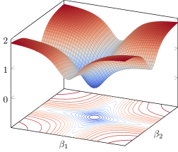
(a) $\gamma^{2}=0.3$

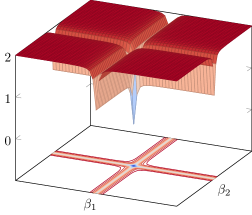
(b) $\gamma^{2}=0.05$

Figure 3: Three-dimensional illustrations of the norm approximation proposed by de Rooi and Eilers (2011) for two different values of $\gamma$. It can be seen that for a smaller value of $\gamma$ the approximation more closely resembles the exact $\ell_{0}$ norm illustrated in Figure 2.

In the following, the approximation will be used to define the SparseStep penalty as

$$P_{\lambda}(\beta_{j})=\lambda\frac{\beta_{j}^{2}}{\beta_{j}^{2}+\gamma^{2}}.$$

To prove that this penalty results in unbiased estimates of the true $\beta_{j}$ parameter, the approach of Fan and Li (2001) is followed. For unbiasedness it is required that the derivative of the penalty term is zero for large values of $\left|\beta_{j}\right|$. The derivative of the SparseStep penalty is

$$P_{\lambda}^{\prime}(\beta_{j})=\lambda\frac{2\gamma^{2}\beta_{j}}{(\beta_{j}^{2}+\gamma^{2})^{2}},$$

hence, it must hold that

$$\lim_{\left|\beta_{j}\right|\rightarrow\infty}P_{\lambda}^{\prime}(\left|\beta_{j}\right|)=\lim_{\left|\beta_{j}\right|\rightarrow\infty}\lambda\frac{2\gamma^{2}\left|\beta_{j}\right|}{(\left|\beta_{j}\right|^{2}+\gamma^{2})^{2}}=0,$$

which is indeed the case, proving that the SparseStep penalty results in unbiased estimates.

Additionally, Fan and Li (2001) derive sufficient conditions for a penalty function to have the Oracle Property. This property means that under certain regularity conditions a method correctly identifies the sparsity in the predictor variables correctly, as the number of observations goes to infinity. One sufficient condition for this is that the derivative of the penalty function should be positive at the origin. This does not hold exactly for SparseStep, but does hold in an arbitrarily small region around the origin, due to the value of $\gamma$. We therefore conjecture that the Oracle Property also holds for SparseStep, but further research is necessary.

The above leads naturally to the formulation of the SparseStep regression problem, with loss function

$$L(\boldsymbol{\beta})=\|\mathbf{y}-\mathbf{X}\boldsymbol{\beta}\|^{2}+\lambda\sum_{j=1}^{m}\frac{\beta_{j}^{2}}{\beta_{j}^{2}+\gamma^{2}}.$$

In the next section, an Iterative Majorization algorithm will be derived for minimizing this loss function.

3 Methodology

With the theoretical underpinnings of SparseStep established above, it is now possible to derive the optimization algorithm necessary to minimize the SparseStep regression loss function. The approach used here is that of the iterative majorization algorithm. A brief introduction is given first, followed by the derivation of the SparseStep algorithm.

3.1 Iterative Majorization

The Iterative Majorization (IM) algorithm is a general optimization algorithm based on surrogate functions, first described by Ortega and Rheinboldt (1970). It is also known as the Majorization Minimization algorithm and is a generalization of the popular Expectation Maximization algorithm (see e.g. Hunter and Lange, 2004). A brief description of the algorithm follows.

Let $f:\mathcal{X}\rightarrow\mathcal{Y}$ with $\mathcal{X}\subseteq\mathbb{R}^{d}$ and $\mathcal{Y}\subseteq\mathbb{R}$ be the function that needs to be optimized. Construct a majorizing function $g:\mathcal{X}\times\mathcal{X}\rightarrow\mathcal{Y}$ such that

$$f(y) =g(y,y),$$

$$f(x) \leq g(x,y)\textrm{ for all }x,y\in\mathcal{X},$$

where $y$ is the so-called supporting point. Differentiability of $f$ at $y$ implies that $\nabla f(y)=\nabla g(y,y)$. Given a majorizing function $g$ the following procedure results in a stationary point of $f$:

1. Let $y=x_{0}$, with $x_{0}$ a starting point

2. Minimize $g(x,y)$ and let $x^{+}=\operatorname*{arg\,min}g(x,y)$

3. Stop if a stopping criterion is reached, otherwise let $y=x^{+}$ and go to step 2.

This procedure yields a guaranteed descent algorithm where $f(x^{+})\leq f(y)$, with a linear convergence rate (De Leeuw, 1994). However, a well-known property of the IM algorithm is that in the first few iterations often large improvements in the loss function can be made (Havel, 1991). This property makes it ideally suited for the SparseStep algorithm described below. Generally, a sufficiently simple functional form is chosen for the majorizing function such that Step 2 in the above procedure can be done swiftly. In the case of the SparseStep regression problem, a quadratic majorizing function is most appropriate.

3.2 Majorization Derivation

The majorizing function of the SparseStep penalty function will be derived here. For ease of notation let $f(x)$ denote the penalty function, with $x\in\mathbb{R}$ and let $g(x,y)$ denote the majorizing function, with $x,y\in\mathbb{R}$. Then,

$$f(x) =\frac{x^{2}}{x^{2}+\gamma^{2}},$$

$$g(x,y) =ax^{2}-2bx+c,$$

where the coefficients of $g(x,y)$ generally depend on $y$. Taking first derivatives yields

$$f^{\prime}(x) =\frac{2x\gamma^{2}}{(x^{2}+\gamma^{2})^{2}},$$

$$g^{\prime}(x,y) =2ax-2b.$$

Since the SparseStep penalty is symmetric, it is desirable that $g(x,y)$ is symmetric as well and thus has its minimum at $x=0$. From this it follows that $g^{\prime}(0,y)=0$, which implies $b=0$. Next, the majorizing function must be tangent to the penalty function at the supporting point $x=y$, thus it is required that $g^{\prime}(y,y)=f^{\prime}(y)$, which yields

$$a =\frac{\gamma^{2}}{(y^{2}+\gamma^{2})^{2}}.$$

Finally, the majorizing function must have the same function value at the supporting point, thus $g(y,y)=f(y)$, this gives

$$\frac{\gamma^{2}}{(y^{2}+\gamma^{2})^{2}}\,y^{2}+c =\frac{y^{2}}{y^{2}+\gamma^{2}}$$

$$c =\frac{y^{4}}{(y^{2}+\gamma^{2})^{2}}.$$

Thus, $g(x,y)$ becomes

$$g(x,y)=\frac{\gamma^{2}}{(y^{2}+\gamma^{2})^{2}}x^{2}+\frac{y^{4}}{(y^{2}+\gamma^{2})^{2}}=\frac{\gamma^{2}x^{2}+y^{4}}{(y^{2}+\gamma^{2})^{2}}.$$

It now remains to be shown that the majorizing function is everywhere above the penalty function, $g(x,y)\geq f(x)$ for all $x\in\mathbb{R}$. This can be done as follows,

$$g(x,y) \geq f(x) \Leftrightarrow$$

$$\frac{\gamma^{2}x^{2}+y^{4}}{(y^{2}+\gamma^{2})^{2}} \geq\frac{x^{2}}{x^{2}+\gamma^{2}} \Leftrightarrow$$

$$(\gamma^{2}x^{2}+y^{4})(x^{2}+\gamma^{2}) \geq x^{2}(y^{2}+\gamma^{2})^{2} \Leftrightarrow$$

$$x^{4}+y^{4}-2x^{2}y^{2} \geq 0 \Leftrightarrow$$

$$(x^{2}-y^{2})^{2} \geq 0. \square$$

Figure 4 shows the majorizing function and the SparseStep penalty function for different values of the supporting point. Note that the majorizing function is indeed symmetric around 0, as desired.

Figure 4: Illustrations of the majorizing function $g(x,y)$ (interrupted lines) of the SparseStep penalty $f(x)$ (solid line), with $\gamma^{2}=0.1$. The majorizing function is shown for various values of the supporting point: the dotted red line at $y=0$, the dash dotted blue line at $y=0.25$, and the dashed green line at $y=0.5$. The vertical lines mark these supporting points for the latter two values.

The above derivation ensures that a majorizing function for the SparseStep loss function can be derived. Recall that the SparseStep loss function is given by

$$L(\boldsymbol{\beta})=\|\mathbf{y}-\mathbf{X}\boldsymbol{\beta}\|^{2}+\lambda\sum_{j=1}^{m}\frac{\beta_{j}^{2}}{\beta_{j}^{2}+\gamma^{2}}.$$

Let $\alpha_{j}$ denote the previous value of $\beta_{j}$ in the IM algorithm (the supporting point). Then, using the majorizing function derived above it is clear that the following inequality holds

$$L(\boldsymbol{\beta})\leq\|\mathbf{y}-\mathbf{X}\boldsymbol{\beta}\|^{2}+\lambda\sum_{j=1}^{m}\frac{\gamma^{2}\beta_{j}^{2}+\alpha_{j}^{4}}{(\alpha_{j}^{2}+\gamma^{2})^{2}}=G(\boldsymbol{\beta},\boldsymbol{\alpha}),$$

where $G(\boldsymbol{\beta},\boldsymbol{\alpha})$ denotes the majorizing function of $L(\boldsymbol{\beta})$. Taking the derivative of $G(\boldsymbol{\beta},\boldsymbol{\alpha})$ with respect to $\boldsymbol{\beta}$ yields an explicit expression for the update of $\boldsymbol{\beta}$ in the IM algorithm. Before taking the derivative of the majorizing function however, let us define

$$\boldsymbol{\Omega}_{jj} =\frac{\gamma^{2}}{(\alpha_{j}^{2}+\gamma^{2})^{2}}$$ (1)

$$\delta_{j} =\alpha_{j}^{2}/\gamma,$$

such that $\boldsymbol{\Omega}$ is an $m\times m$ diagonal matrix with elements $\boldsymbol{\Omega}_{jj}$ and $\boldsymbol{\delta}\in\mathbb{R}^{m}$ a vector with elements $\delta_{j}$. With these definitions, the regularization term becomes

$$\lambda\sum_{j=1}^{m}\frac{\gamma^{2}\beta_{j}^{2}+\alpha_{j}^{4}}{(\alpha_{j}^{2}+\gamma^{2})^{2}}=\lambda(\boldsymbol{\beta}^{\prime}\boldsymbol{\Omega}\boldsymbol{\beta}+\boldsymbol{\delta}^{\prime}\boldsymbol{\Omega}\boldsymbol{\delta}).$$

By expanding the norm and using this form for the regularization term, it is possible to write $G(\boldsymbol{\beta},\boldsymbol{\alpha})$ as

$$G(\boldsymbol{\beta},\boldsymbol{\alpha})=\mathbf{y}^{\prime}\mathbf{y}-2\mathbf{y}^{\prime}\mathbf{X}\boldsymbol{\beta}+\boldsymbol{\beta}^{\prime}(\mathbf{X}^{\prime}\mathbf{X}+\lambda\boldsymbol{\Omega})\boldsymbol{\beta}+\lambda\boldsymbol{\delta}^{\prime}\boldsymbol{\Omega}\boldsymbol{\delta}.$$

Taking the derivative to $\boldsymbol{\beta}$ and setting this to zero, yields

$$-2\mathbf{X}^{\prime}\mathbf{y}+2(\mathbf{X}^{\prime}\mathbf{X}+\lambda\boldsymbol{\Omega})\boldsymbol{\beta}=0$$

Thus, the update of the majorization algorithm is simply

$$\boldsymbol{\beta}=\left(\mathbf{X}^{\prime}\mathbf{X}+\lambda\boldsymbol{\Omega}\right)^{-1}\mathbf{X}^{\prime}\mathbf{y}.$$

Since $\boldsymbol{\Omega}$ is a diagonal matrix this expression is remarkably similar to the solution of the ridge regression problem, in which $\boldsymbol{\Omega}$ is simply the identity matrix.

3.3 SparseStep Algorithm

With the derivation of the IM algorithm for minimizing the SparseStep regression loss function, it is now possible to formulate the SparseStep algorithm. To avoid local minima, the SparseStep penalty is introduced slowly by starting with a large value of $\gamma$, so that the penalty is very smooth and behaves like a ridge penalty. Then, the $\gamma$ value is reduced so that the irregularity and nonconvexity is introduced slowly. The value of $\gamma$ is reduced until it is close to zero. By slowly introducing the nonsmoothness in the penalty and taking only a few steps of the IM algorithm for each $\gamma$, the SparseStep algorithm aims to avoid local minima and tries to reach the global minimum of the regression problem with the counting norm penalty. The pseudocode for SparseStep regression is given in Algorithm 1.

The algorithm starts by initializing $\boldsymbol{\beta}$ and $\gamma$ from given values $\boldsymbol{\beta}_{0}$ and $\gamma_{0}$ respectively. For each value of $\gamma$ the parameter estimates are updated $t_{max}$ times using the IM algorithm. Subsequently $\gamma$ is reduced by a factor $\gamma_{step}$. This process is continued until $\gamma$ reaches a provided stopping value $\gamma_{stop}$. In the end, sufficiently small elements of $\boldsymbol{\beta}$ are set to absolute zero by comparing to a small constant $\epsilon$. This is done to avoid numerical precision errors and can be a method for enhancing the sparsity inducing properties of SparseStep. The value of $\epsilon$ and that of $\gamma_{stop}$ are related. Note that in an actual implementation the matrices $\mathbf{X}^{\prime}\mathbf{X}$ and $\mathbf{X}^{\prime}\mathbf{y}$ should be cached for computational efficiency.

Algorithm 1 SparseStep Regression

  Input: $\mathbf{X}$, $\mathbf{y}$, $\boldsymbol{\beta}_{0}$, $\gamma_{0}$, $\gamma_{stop}$, $\gamma_{step}$, $t_{max}$, $\epsilon$

  Output: $\boldsymbol{\beta}$

  $\boldsymbol{\beta}\leftarrow\boldsymbol{\beta}_{0}$

  $\gamma\leftarrow\gamma_{0}$

  while $\gamma>\gamma_{stop}$ do

     for $t=1$ to $t_{max}$ do

        Construct $\boldsymbol{\Omega}$ according to (1)

        $\boldsymbol{\beta}\leftarrow\left(\mathbf{X}^{\prime}\mathbf{X}+\lambda\boldsymbol{\Omega}\right)^{-1}\mathbf{X}^{\prime}\mathbf{y}$

     end for

     $\gamma\leftarrow\gamma/\gamma_{step}$

  end while

  for $j\in\{1,\ldots,m\}$ do

     if $|\beta_{j}|<\epsilon$ then

        $\beta_{j}\leftarrow 0$

     end if

  end for

4 Experiments

To verify the performance of the SparseStep algorithm in correctly identifying the nonzero predictor variables in a regression problem, a simulation study was performed. The aim of this simulation study is to mimic as much as possible a practical setting where a researcher is interested in both the predictive accuracy of a regression model and the correct identification of variables with nonzero coefficients. Moreover, this simulation study allows verification of the performance of the SparseStep algorithm for datasets with varying statistical properties such as the number of variables, the signal-to-noise ratio (SNR), the correlation between the variables, and the degree of sparsity in the true coefficient vector.

A second goal of this simulation study is to compare the performance of the SparseStep algorithm with existing regression methods. These competing methods are: ordinary least-squares, lasso (Tibshirani, 1996), ridge regression (Hoerl and Kennard, 1970), SCAD (Fan and Li, 2001), and MC+ (Zhang, 2010). Thus, the focus here is on comparing SparseStep with other penalized regression methods, including some that induce sparsity through penalization. In order to accurately evaluate the predictive accuracy of these methods and to find the best regularization parameter for each method, separate training and testing datasets will be used. The procedure is then to find for each method the regularization parameter which performs best on the training dataset, as measured using 10-fold cross-validation. Next, each method is trained one more time on the entire training dataset using this optimal regularization parameter and the obtained model is used to predict the test dataset. Predictive accuracy is measured using the mean squared error (MSE) on the test dataset.

The accuracy of the estimated parameter vector ${\boldsymbol{\hat{\beta}}}$ will be evaluated on two measures: the mean squared error with respect to the true $\boldsymbol{\beta}$ and the sparsity hitrate. The sparsity hitrate is calculated simply as the sum of the correctly identified zero elements of $\boldsymbol{\beta}$ and the correctly identified nonzero elements, divided by the total number of elements of $\boldsymbol{\beta}$.

For the simulation study the following data generating process will be used. Let $\mathbf{X}\in\mathbb{R}^{n\times m}$ denote the data matrix drawn from a multivariate normal distribution with mean vector $\boldsymbol{\mu}\in\mathbb{R}^{m}$ and correlation matrix $\boldsymbol{\Sigma}\in\mathbb{R}^{m\times m}$, such that the rows $\mathbf{x}_{i}^{\prime}\sim\mathcal{N}(\boldsymbol{\mu},\boldsymbol{\Sigma})$. The data matrix $\mathbf{X}$ was scaled such that each column had mean 0 and unit variance. In all simulated datasets $\boldsymbol{\mu}$ is drawn from an $m$-dimensional standard uniform distribution. For the correlation matrix $\boldsymbol{\Sigma}$ three different scenarios are used: uncorrelated, constantly correlated, and noise correlated. In the uncorrelated case the $\boldsymbol{\Sigma}$ matrix is simply the identity matrix, in the constantly correlated case all variables have a correlation of .5 with each other, whereas in the noise correlated case a correlation matrix is generated by adding realistic noise to the identity matrix using the method of Hardin et al. (2013). Next, a parameter vector $\boldsymbol{\beta}\in\mathbb{R}^{m}$ is drawn from a uniform distribution with elements $\beta_{j}\in[-1,1]$. The last $z$ elements of $\boldsymbol{\beta}$ are set to zero to simulate sparsity. Finally, to obtain realistic data with a known signal-to-noise ratio, the simulated outcome variable $\mathbf{y}$ is calculated as

$$\mathbf{y}=\mathbf{X}\boldsymbol{\beta}+\mathbf{e},$$

where $\mathbf{e}\in\mathbb{R}^{n}$ is a noise term which contains $n$ elements drawn from a univariate normal distribution with mean zero and standard deviation such that the SNR given by $\boldsymbol{\beta}^{\prime}\mathbf{X}^{\prime}\mathbf{X}\boldsymbol{\beta}/\mathbf{e}^{\prime}\mathbf{e}$ is as desired.

Table 1: Overview of the values for different parameters in the data generating process of the simulation study. Datasets were generated for each possible combination of these values, resulting in 180 datasets.

Parameter	Values
Variables ($m$)	$10,50,100,500$
Sparsity ($\zeta\%$)	$0,25,50,75,95$
SNR	$0.1,1.0,10.0$
Correlation	uncorrelated, constant, noise

Table 1 gives an overview of how the different parameters of the data generating process were varied among datasets. Using these parameters a total of 180 datasets were generated. For all datasets the number of instances $n$ was set to 30,000, which was then split into 20,000 instances in the training dataset and 10,000 in the testing dataset. Note that the degree of sparsity in the table is expressed as a percentage of the number of variables $m$. In practice, the number of zeroes in $\boldsymbol{\beta}$ corresponds to $z=\lfloor m\cdot\zeta/100\rfloor$, where $\zeta$ is a number taken from the second row of the table.

The simulation study was set up such that each method was trained on exactly the same cross-validation sample when the same value of $\lambda$ was supplied. The grid of $\lambda$ parameters for the regularized methods came from a logarithmically spaced vector of 101 values between $2^{-15}$ and $2^{15}$. For SparseStep, the input parameters were chosen as $\gamma_{0}=10^{6}$, $\gamma_{stop}=10^{-8}$, $\gamma_{step}=2$, $t_{max}=2$, $\epsilon=10^{-7}$, and $\boldsymbol{\beta}_{0}=\mathbf{0}$ (see Algorithm 1). Default input parameters where chosen for the other methods where applicable. The R language (R Core Team, 2015) was used for the SCAD and MC+ methods, with SCAD implemented through the ncvreg package (Breheny and Huang, 2011), and MC+ through the SparseNet package (Mazumder et al., 2011). The other methods were implemented in the Python language (van Rossum, 1995) using the scikit-learn package (Pedregosa et al., 2011). For the MC+ penalty the secondary regularization parameter $a$ was optimized for the training dataset using the CV implementation of the SparseNet package. For SCAD $a$ was set to 3.7 as per the default settings of ncvreg and Fan and Li (2001).

To determine statistically significant differences between the performance of each of the methods, recommendations on benchmarking machine learning methods will be used as formulated by Demšar (2006). Specifically, rank tests will be applied to evaluate whether SparseStep outperforms other methods significantly. For each dataset, fractional ranks are calculated for each performance measure with a smaller rank indicating a better performance. Methods are considered to have equal performance if the difference on a performance metric is smaller than $10^{-4}$. A Friedman rank test can be done on the calculated ranks to test for equal performance of the methods (Friedman, 1937, 1940) and Holm’s step down procedure can be used to test for significant differences between SparseStep and other methods (Holm, 1979).

Figure 5 shows the average ranks of the six evaluated methods on four different metrics. From Figure 5(a), which shows the average ranks on the MSE of $\boldsymbol{\hat{\beta}}$, it can be seen that SparseStep is most often the best method for fitting $\boldsymbol{\beta}$, followed closely by SCAD, MC+, and the Lasso. The sparsity hitrate of $\boldsymbol{\hat{\beta}}$ is on average the best for the MC+ penalty, followed by SparseStep and SCAD, as illustrated in Figure 5(b). For the out-of-sample performance on the test data, shown in 5(c), a similar order of the methods can be observed as for the MSE on $\boldsymbol{\hat{\beta}}$, although the difference between SCAD and MC+ is larger here. SparseStep again outperforms the other methods on this measure.

(a) MSE of $\boldsymbol{\hat{\beta}}$

(b) Sparsity hitrate $\boldsymbol{\hat{\beta}}$

(c) MSE of $\mathbf{\hat{y}}$ on test datasets

(d) Average computation time

Figure 5: Rank plots showing the average performance of the six evaluated methods on the 180 simulated datasets. Points on the line show the fractional rank of the methods averaged over all datasets, with a smaller rank indicating a better performance. It can therefore be seen that SparseStep performs very favorably in both predicting the size and sparsity of $\boldsymbol{\beta}$, as well as on predicting the outcome out-of-sample. Graph (d) shows the rank graph for the average computation time for each method.

Computation time was also measured for each method on each dataset. The rank plot of the average computation time per dataset is given in Figure 5(d). It can be seen that SparseStep performs well on average. The average computation time of SparseStep for a single value of $\lambda$ is comparable to computing a single OLS solution. An important caveat with regards to the computation times is that in order to have the same CV splits for each method with a certain $\lambda$, the path algorithms of the Lasso, SCAD, and MC+ penalty could not be used. The computation time of these methods is therefore overestimated.

Apart from the ranks averaged over all datasets, it is also interesting to look at how often a method is the best method on a dataset and how often it is the worst method. Looking at the MSE of $\boldsymbol{\hat{\beta}}$, Ridge is most often the best method, followed closely by the penalized methods. As expected OLS is most often the worst method in this regard. Next, SparseStep most often obtains the highest sparsity hitrate of $\boldsymbol{\beta}$, on 30 out of 180 datasets. MC+ is the best method on this metric on 26 datasets and SCAD on 11 datasets. Finally, when considering the MSE on the outcome of the test dataset all the penalized methods are the best method with similar frequency. An exception to this is OLS, which is the best method on only 7 datasets and the worst method on 52 of them. MC+ is the worst method on 32 datasets, whereas SparseStep is the worst method the smallest number of times, on only 6 datasets. Clearly, OLS and Ridge only perform well on datasets without sparsity in $\boldsymbol{\beta}$. For the other methods no clear relationship between the dataset characteristics and the performance of the method could be found.

As suggested by Demšar (2006) an $F$-test can be done on the average ranks to evaluate if significant differences exist between the different methods. This is the case for the four measures discussed above, all with p-value $<0.0001$. Furthermore, Holm’s procedure can be performed to uncover significant differences between the methods and a reference method, in this case SparseStep. From this it is found that on the performance metrics other than computation time, SparseStep significantly outperforms OLS and Ridge, but that the difference between SparseStep and the other penalized methods is not significant at the 5% level. On the computation time metric SparseStep significantly outperforms SCAD and MC+ at the 5% level, but the caveat mentioned above should be taken into account here. The lack of a significant difference between SparseStep and SCAD and MC+ on the other metrics can be due to either a lack of any theoretical difference, or an insufficient number of datasets in the simulation study.

5 Discussion

This paper introduces the SparseStep algorithm which induces sparsity in the regression problem by iteratively improving an approximation of the $\ell_{0}$ norm. An iterative majorization algorithm has been derived which is straightforward to implement. The practical relevance of SparseStep is evaluated through a thorough simulation study on 180 datasets with varying characteristics. Results of the simulation study indicate that SparseStep often outperforms existing methods, both for identifying the parameter vector $\boldsymbol{\beta}$ as for out-of-sample prediction of the outcome variable. Future research will focus on furthering the understanding of the theoretical properties of the SparseStep algorithm, such as the criteria for convergence to a global optimum.

References

- Breheny and Huang [2011] P. Breheny and J. Huang. Coordinate descent algorithms for nonconvex penalized regression, with applications to biological feature selection. The Annals of Applied Statistics, 5(1):232, 2011.
- De Leeuw [1994] J. De Leeuw. Block-relaxation algorithms in statistics. In Information systems and data analysis, pages 308–324. Springer, 1994.
- de Rooi and Eilers [2011] J. de Rooi and P. Eilers. Deconvolution of pulse trains with the penalty. Analytica Chimica Acta, 705(1):218–226, 2011.
- Demšar [2006] J. Demšar. Statistical comparisons of classifiers over multiple data sets. The Journal of Machine Learning Research, 7:1–30, 2006.
- Donoho [2006] D.L. Donoho. Compressed sensing. Information Theory, IEEE Transactions on, 52(4):1289–1306, 2006.
- Fan and Li [2001] J. Fan and R. Li. Variable selection via nonconcave penalized likelihood and its oracle properties. Journal of the American statistical Association, 96(456):1348–1360, 2001.
- Friedman [1937] M. Friedman. The use of ranks to avoid the assumption of normality implicit in the analysis of variance. Journal of the American Statistical Association, 32(200):675–701, 1937.
- Friedman [1940] M. Friedman. A comparison of alternative tests of significance for the problem of rankings. The Annals of Mathematical Statistics, 11(1):86–92, 1940.
- Hardin et al. [2013] J. Hardin, S. R. Garcia, and D. Golan. A method for generating realistic correlation matrices. The Annals of Applied Statistics, 7(3):1733–1762, 2013.
- Hastie et al. [2009] T. Hastie, R. Tibshirani, and J. Friedman. The Elements of Statistical Learning. Springer, New York, 2nd edition, 2009.
- Havel [1991] T. F. Havel. An evaluation of computational strategies for use in the determination of protein structure from distance constraints obtained by nuclear magnetic resonance. Progress in Biophysics and Molecular Biology, 56(1):43–78, 1991.
- Hoerl and Kennard [1970] A. E. Hoerl and R. W. Kennard. Ridge regression: Biased estimation for nonorthogonal problems. Technometrics, 12(1):55–67, 1970.
- Holm [1979] S. Holm. A simple sequentially rejective multiple test procedure. Scandinavian Journal of Statistics, 6(2):65–70, 1979.
- Hunter and Lange [2004] D. R. Hunter and K. Lange. A tutorial on MM algorithms. The American Statistician, 58(1):30–37, 2004.
- Mazumder et al. [2011] R. Mazumder, J.H. Friedman, and T. Hastie. SparseNet: Coordinate descent with nonconvex penalties. Journal of the American Statistical Association, 106(495), 2011.
- Natarajan [1995] B. K. Natarajan. Sparse approximate solutions to linear systems. SIAM Journal on Computing, 24(2):227–234, 1995.
- Ortega and Rheinboldt [1970] J.M. Ortega and W.C. Rheinboldt. Iterative Solutions of Nonlinear Equations in Several Variables. New York: Academic Press, 1970.
- Pedregosa et al. [2011] F. Pedregosa, G. Varoquaux, A. Gramfort, V. Michel, B. Thirion, O. Grisel, M. Blondel, P. Prettenhofer, R. Weiss, V. Dubourg, J. Vanderplas, A. Passos, D. Cournapeau, M. Brucher, M. Perrot, and E. Duchesnay. Scikit-learn: Machine learning in Python. The Journal of Machine Learning Research, 12:2825–2830, 2011.
- Peetre and Sparr [1972] J. Peetre and G. Sparr. Interpolation of normed abelian groups. Annali di Matematica Pura ed Applicata, 92(1):217–262, 1972.
- R Core Team [2015] R Core Team. R: A Language and Environment for Statistical Computing. R Foundation for Statistical Computing, Vienna, Austria, 2015.
- Tibshirani [1996] R. Tibshirani. Regression shrinkage and selection via the lasso. Journal of the Royal Statistical Society. Series B (Methodological), 58(1):267–288, 1996.
- van Rossum [1995] G. van Rossum. Python tutorial. Technical Report CS-R9526, CWI (Centre for Mathematics and Computer Science), Amsterdam, The Netherlands, 1995.
- Zhang [2010] C.-H. Zhang. Nearly unbiased variable selection under minimax concave penalty. The Annals of Statistics, 38:894–942, 2010.