Observational effects of varying speed of light in quadratic gravity cosmological models

Abstract

We study different manifestations of the speed of light in theories of gravity where metric and connection are regarded as independent fields. We find that for a generic gravity theory in a frame with locally vanishing affine connection, the usual degeneracy between different manifestations of the speed of light is broken. In particular, the space–time causal structure constant ($c_{ST}$) may become variable in that local frame. For theories of the form $f(\mathcal{R},\mathcal{R}^{\mu\nu}\mathcal{R}_{\mu\nu})$, this variation in $c_{ST}$ has an impact on the definition of the luminosity distance (and distance modulus), which can be used to confront the predictions of particular models against Supernovae type Ia (SN Ia) data. We carry out this test for a quadratic gravity model without cosmological constant assuming i) a constant speed of light and ii) a varying speed of light, and find that the latter scenario is favored by the data.
Keywords:   Palatini formalism, Modified gravity, Causal structure constant, Varying speed of light.

1 Introduction

One of the major challenges faced by current cosmological models is the late-time accelerating expansion of the universe. According to the extensive observational evidence based on Type Ia supernovae (SN Ia) [1, 2], and standard rulers [3, 4], our universe seems to be undergoing an accelerating expansion phase. In order to explain this phenomenon, two general classes of models have been put forward. In the first class, the acceleration is attributed to new energy sources with repulsive gravitational properties, which is dubbed dark energy. The second class of models seeks for self-accelerating solutions of the field equations by modifying the dynamics of general relativity (GR) on purely geometrical grounds or through the interpretation of cosmological observations from a different perspective [5].

The second approach offers a variety of alternatives to modify Einstein’s theory of gravity. These fall into different categories such as scalar-tensor theories, tensor-vector-scalar theories, higher dimensional theories, theories with modified Lagrangians of the type $f(\mathcal{R},\mathcal{R}^{\mu\nu}\mathcal{R}_{\mu\nu})$, extensions that consider non-minimal matter-curvature couplings, and even more exotic alternatives. In addition, all these theories can be investigated in different variational scenarios, such as the (usual) metric approach, the Palatini/metric-affine formalism [6, 7, 8, 4], and also from a hybrid metric-Palatini perspective [9].

When extensions of the standard model for gravity are considered, special attention should be paid to the origin and role of some fundamental constants. In particular, in metric-affine scenarios, where the metric and affine structures are a priori independent, it is necessary to clarify the different roles that the speed of light might play. This opens the possibility of distinguishing between several inequivalent manifestations which are degenerate in the framework of GR [10]. In this sense, one must distinguish between the following:

• $c_{ST}$ : the space–time causal structure constant, which appears in the space-time line element and determines the local null cones.

• $c_{GW}$ : the velocity that appears in the equations that describe gravitational waves.

• $c_{EM}$ : the velocity that appears in electromagnetic waves equation.

• $c_{E}$ : the gravity-matter coupling constant appearing on the right-hand side of Einstein’s equations.

To the above, one could also add the clock synchronization speed $(c_{C})$, which is the speed of the signal used to synchronize faraway clocks. Assuming Maxwell’s electrodynamics and Einstein’s gravity, the Newtonian limit requires $\frac{c_{E}}{c_{0}}=\frac{c_{GW}}{c_{0}}=\frac{c_{EM}}{c_{0}}=\frac{c_{ST}}{c_{0}}=1$, where $c_{0}$ is a constant with dimensions, which we choose as $3\times 10^{8}m/s$ in MKS units.

It should be noted that beyond the Newtonian approximation there is no compelling reason to consider all the above manifestations of the speed of light to be the same in all theories and formalisms inasmuch as this quantity appears in many physical laws with different and a priori unrelated origins.

In the context of Palatini/metric-affine theories, the existence of a connection a priori independent of the metric puts forward that the $c_{ST}$ associated to the frames in which the metric is locally Minkowskian does not need to be the same as the quantity in a frame, in which the geodesics of the independent connection appear as straight lines. This is rather obvious for those cases in which there exists a nontrivial non-metricity tensor $Q_{\alpha\mu\nu}\equiv\nabla_{\alpha}^{\Gamma}g_{\mu\nu}$, where $\nabla_{\alpha}^{\Gamma}$ denotes the covariant derivative of the independent connection. Given that $Q_{\alpha\mu\nu}$ is a tensor, the local coordinate transformation that brings the metric into Minkowskian form does not force the $Q_{\alpha\mu\nu}$ to vanish at the same time. As a consequence, though the Christoffel symbols ${\alpha\brace\mu\nu}$ of the metric vanish in those coordinates, the connection coefficients $\Gamma^{\alpha}_{\mu\nu}={\alpha\brace\mu\nu}-\frac{g^{\alpha\lambda}}{2}\left(Q_{\mu\lambda\nu}+Q_{\nu\lambda\mu}-Q_{\lambda\mu\nu}\right)$ do not, in general. Thus, locally $c_{ST}$ could be different from the propagation speed of light rays.

In relation to this, the velocity of gravitational waves, $c_{GW}$ is another magnitude that deviates from the usual speed of light in theories beyond GR. In the case of Palatini theories whose Lagrangian is based on the metric and the Ricci tensor, it was recently shown that tensorial perturbations in cosmological scenarios satisfy an equation formally identical to that found in GR, in which the background variables represent the auxiliary metric associated to the independent connection [11]. This means that in the geometrical optics approximation, these gravitational waves follow the geodesics of $\Gamma^{\alpha}_{\mu\nu}$ rather than those of ${\alpha\brace\mu\nu}$. Though cosmological backgrounds of gravitational waves are not yet accessible to observation, the recent direct detection of aLIGO [12] opens a new window on the exploration of this new source of radiation and, in particular, for measuring and testing $\frac{c_{GW}}{c_{EM}}$ [13, 14].

The main purpose of this work, therefore, is to explore the impact of relaxing the universality of the different manifestations of the speed of light in the definition of cosmological distances in the modified gravity scenario of Palatini extensions of GR. For concreteness, we will consider $f(\mathcal{R})$ and $f(\mathcal{R},\mathcal{R}_{(\mu\nu)}\mathcal{R}^{(\mu\nu)})$ theories with minimal matter couplings. We will comment on the different forms in which the speed of light enters in the equations that describe the background evolution of these theories and use observational data to study the effect of a varying speed of light on the supernovae luminosity distance. This analysis will allow us to determine if it is possible to find a modified gravity model with a varying speed of light able to fit the supernovae data and be in good agreement with the concordance model results without explicitly considering a cosmological constant or sources of dark energy.

2 Speed of light in metric-affine theories

In a very lucid work, Ellis and Uzan [10] presented different scenarios in which a quantity with dimensions of squared velocity appears and is typically interpreted as the same magnitude, namely, the speed of light. This assumption is nontrivial and comparable to the equivalence between inertial and gravitational mass. A deeper understanding of the latter led Einstein to formulate his now well accepted equivalence principle. A careful analysis of the different facets of the speed of light could lead also to a better understanding of the scenarios where it appears and their interrelations.

Though the relativistic formulation of physical laws was motivated by properties of the electromagnetic field, it is now well understood that the principle of relativity transcends Maxwell’s theory and affects all the other known interactions. In this sense, the limiting speed $c_{ST}$ that determines the causal structure of Minkowski space-time, $ds^{2}=c_{ST}^{2}dt^{2}-d\vec{x}^{2}$, needs not be the same as the speed $c_{EM}$ that appears in the equations for electromagnetic waves. The speed of light that appears on the right-hand side of Einsteins equations may also, in principle, be different from $c_{EM}$ and $c_{ST}$. These examples put forward that a careful analysis of the different facets typically attributed to the speed of light is necessary.

The above discussion becomes particularly relevant in gravitational scenarios where the metric and affine structures of space-time are regarded as a priori independent. In such theories the local value of $c_{ST}$ may be subject to variation depending on how local observers are defined. This definition must be addressed carefully, as the dynamics of these theories may introduce operational subtleties not perceived in a purely kinematical analysis. To see this, let us consider first the kinematic description. In this approach, one may take the viewpoint that local measurements are performed by observers for which the geodesics of the metric $g_{\mu\nu}$ appear as straight lines around a given point. This simply requires performing a nonlinear coordinate transformation such that the original Christoffel symbols ${\alpha\brace\mu\nu}$ of the metric vanish. With an additional (linear) change of coordinates, $g_{\mu\nu}$ can be made Minkowskian at the chosen point, with the leading order corrections generated by the external matter fields being quadratic in the background curvature. If the total energy of the local gravitating system is small, then the Minkowskian approximation is valid locally in those coordinates. Alternatively, one may consider the family of local observers for which the geodesics of the independent connection, $\Gamma^{\alpha}_{\beta\gamma}$, are straight lines. In this case it is also possible to make the metric look locally Minkowskian by considering a local linear transformation that preserves the condition $\Gamma^{\alpha}_{\beta\gamma}=0$. Thus, it seems possible, in principle, to make the metric look Minkowskian at any desired point regardless of whether the connection is metric-compatible (Christoffel symbols of $g_{\mu\nu}$) or not. Obviously, the relation between the coordinates that make ${\alpha\brace\mu\nu}=0$ and those for which $\Gamma^{\alpha}_{\beta\gamma}=0$ is nonlinear, which implies that they have a certain relative acceleration (determined by the tensor $\Gamma^{\alpha}_{\beta\gamma}-{\alpha\brace\beta\gamma}$). In other words, if one picks up a frame where only the Christoffel symbol of the metric is zero at some point, then the full Riemann tensor would not be zero at that point.

Now, the point is that once the dynamical relation between $g_{\mu\nu}$ and $\Gamma^{\alpha}_{\beta\gamma}$ is obtained, it is not immediate to guarantee that the Minkowskian condition can always be satisfied locally for $g_{\mu\nu}$. An explanation is in order. In these theories, one typically finds that $\Gamma^{\alpha}_{\beta\gamma}$ can be written as the Christoffel symbols of an auxiliary metric $h_{\mu\nu}$. This $h_{\mu\nu}$ is governed by a set of equations of the form ${\mathcal{R}_{\mu}}^{\nu}(h)={\tau_{\mu}}^{\nu}$, where ${\mathcal{R}_{\mu}}^{\nu}(h)=R_{\mu\alpha}h^{\alpha\nu}$, $\mathcal{R}_{\mu\alpha}$ is the Ricci tensor of $h_{\mu\nu}$, and ${\tau_{\mu}}^{\nu}$ represents an effective stress-energy tensor which is completely determined by $h_{\mu\nu}$ and the matter fields. This implies that locally (or in the absence of external gravitational fields) any departure of $h_{\mu\nu}$ from $\eta_{\mu\nu}$ is determined by an integration over the local matter sources, i.e., by the total energy of the local system (similarly as in GR). The point is that the relation between $h_{\mu\nu}$ and $g_{\mu\nu}$ depends on the local stress-energy density via a transformation of the form $g_{\mu\nu}={{\Omega^{-1}}_{\mu}}^{\alpha}h_{\alpha\nu}$, with ${{\Omega^{-1}}_{\mu}}^{\alpha}$ specified by the stress-energy tensor of the local sources. For $f(\mathcal{R})$ theories, for instance, ${{\Omega^{-1}}_{\mu}}^{\alpha}=\frac{1}{f_{\mathcal{R}}(T)}{\delta_{\mu}}^{\alpha}$, where $f_{\mathcal{R}}=df/d\mathcal{R}$ and the dependence on the trace $T$ of the stress-energy tensor is determined by the equation $\mathcal{R}f_{\mathcal{R}}-2f(\mathcal{R})=\kappa^{2}T$. Thus, if the total energy-momentum of a local system is small but its stress-energy density distribution is not negligible, one could only justify that $h_{\mu\nu}\approx\eta_{\mu\nu}$ but $g_{\mu\nu}\approx\frac{1}{f_{\mathcal{R}}(T)}\eta_{\mu\nu}$. This property has been used to rule out models with inverse curvature terms due to nontrivial effects on atomic systems [16, 17, 18]. Obviously, at every single point of the local system (in space and in time) one could find a coordinate transformation that removes the density dependence from the metric at that instant and location. However, the notion of observer as a point-like, structureless entity is not valid in this context. For extended sources with fluctuating stress-energy tensor or for regions crossed by different radiation fields, such a local (point-like, structureless) and instantaneous choice of coordinates is of no use. One can thus, at most, screen the external effects of gravity by the choice of a frame in which $h_{\mu\nu}$ appears as Minkowskian. The effects of the local stress-energy density, however, cannot be eliminated in that way.

Turning back to the definition of $c_{ST}$, one finds that in the case of $f(\mathcal{R})$ theories, $c_{ST}$ is insensitive to the form of the function $f_{\mathcal{R}}(T)$ because the two metrics are conformally related. In other metric-affine theories, such as in the case of quadratic gravity, $\mathcal{R}+\alpha\mathcal{R}^{2}+\beta\mathcal{R}_{(\mu\nu)}\mathcal{R}^{(\mu\nu)}$, or in Born-Infeld inspired gravity models, the deformation matrix ${{\Omega^{-1}}_{\mu}}^{\alpha}$ has two (or more) different eigenvalues, which induces nontrivial modifications in $c_{ST}$. As discussed in [19, 20] for FLRW cosmological models driven by perfect fluids in gravity theories of the form $\mathcal{R}+f(\mathcal{R}^{\mu\nu}\mathcal{R}_{\mu\nu})$, one finds ${{\Omega^{-1}}_{\mu}}^{\alpha}=\text{diag}(1/(\lambda\omega),1/\lambda,1/\lambda,1/\lambda)$, where $\lambda$ and $\omega$ are functions of the fluid pressure and energy density, which are functions of cosmic time. In the local frame $e^{\mu}_{a}$ in which $h_{\mu\nu}e^{\mu}_{a}e^{\nu}_{b}=\eta_{ab}$, one has $g_{\mu\nu}e^{\mu}_{a}e^{\nu}_{b}=\text{diag}(1/(\lambda\omega),-1/\lambda,-1/\lambda,-1/\lambda)$. As a result, the line element $ds^{2}=g_{\mu\nu}dx^{\mu}dx^{\nu}$ becomes $ds^{2}=c_{0}^{2}dt^{2}-d\vec{x}^{2}$ in its own local frame but turns into $ds^{2}=c_{0}^{2}/(\lambda\omega)dt^{2}-d\vec{x}^{2}/\lambda$ in the local frame of $h_{\mu\nu}$. Thus, in the $h$-frame, we have $c_{ST}^{2}=c_{0}^{2}/\omega$. This puts forward that $c_{ST}$ may be subject to a time variation induced by the evolution of the cosmic expansion and modulated by the specific form of the gravity Lagrangian.

3 Dynamics of Palatini $f(\mathcal{R})$ and $f(\mathcal{R},\mathcal{R}^{\mu\nu}\mathcal{R}_{\mu\nu})$ theories

For the sake of concreteness, in this section we study two well-known families of theories whose Lagrangians are arbitrary functions of the form $f(\mathcal{R})$ and $f(\mathcal{R},\mathcal{R}^{\mu\nu}\mathcal{R}_{\mu\nu})$ (from now on we assume symmetrization of the indices in the Ricci tensor). Their field equations will be derived assuming that metric and connection are independent. For simplicity in the discussion, we will consider $c_{E}=c_{0}$ so that $\kappa=\frac{8\pi G}{c_{0}^{4}}$.

The Lagrangian density of the non-linear Ricci scalar gravity model is chosen to be an arbitrary function of the scalar curvature,

$$\mathcal{L}=\frac{1}{2\kappa}f(\mathcal{R}[g,\Gamma])+\mathcal{L}_{m}$$ (1)

in which $\kappa=8\pi G/c_{0}^{4}$, and the matter Lagrangian density, $\mathcal{L}_{m}$, does not depend on the connection for simplicity. Variation of the action leads to

$$f^{\prime}(\mathcal{R})\mathcal{R}_{\mu\nu}-\frac{1}{2}f(\mathcal{R})g_{\mu\nu}=\kappa T_{\mu\nu}\ ,$$ (2)

whose trace with respect to the metric yields the algebraic relation $\mathcal{R}f_{\mathcal{R}}-2f=\kappa T$. The connection equation can be simplified to

$$\nabla_{\alpha}^{\Gamma}\left(\sqrt{-g}f^{\prime}g^{\mu\nu}\right)=0\ ,$$ (3)

where $\nabla_{\mu}^{\Gamma}X^{\nu}=\partial_{\mu}X^{\nu}+\Gamma^{\nu}_{\alpha\mu}X^{\alpha}$. It is easy to verify that the connection that solves this last equation coincides with the Levi-Civita connection of a metric $h_{\mu\nu}=f^{\prime}g_{\mu\nu}$, such that

$$\Gamma^{\alpha}_{\mu\nu}={\alpha\brace\mu\nu}+\gamma^{\alpha}_{\mu\nu}={\alpha\brace\mu\nu}+\frac{1}{2f^{\prime}}\left[2\delta^{\alpha}_{(\mu}\partial_{\nu)}f^{\prime}-g_{\mu\nu}g^{\alpha\beta}\partial_{\beta}f^{\prime}\right]\ .$$ (4)

For the case of $f(\mathcal{R},\mathcal{R}_{\mu\nu}\mathcal{R}^{\mu\nu})=\mathcal{R}+f(\mathcal{R}^{\mu\nu}\mathcal{R}_{\mu\nu})$ theories, it can be shown that variation of the action with respect to the metric and the independent affine connection leads to [15]

$$\mathcal{R}_{\mu\nu}+2F\mathcal{R}_{\mu}^{\alpha}\mathcal{R}_{\nu\alpha}-\frac{1}{2}g_{\mu\nu}[\mathcal{R}+f]=\kappa T_{\mu\nu}$$ (5)

$$\nabla_{\sigma}^{\Gamma}\left[\sqrt{-g}(g^{\mu\nu}+2Fg^{\mu\alpha}\mathcal{R}_{\alpha\beta}g^{\nu\beta})\right]=0\ .$$ (6)

After ADM decomposition, the energy–momentum tensor can be written as below [19, 21]:

$$T_{\mu\nu}=\rho u_{\mu}u_{\nu}+2q_{(\mu}u_{\nu)}-p\tilde{g}_{\mu\nu}+\pi_{\mu\nu},$$ (7)

in which $u^{\mu}=\frac{dx^{\mu}}{d\tau}$ is the 4-velocity normalized as $u^{\mu}u_{\mu}=1$, $\tilde{g}_{\mu\nu}=g_{\mu\nu}-u_{\mu}u_{\nu}$ which determines the orthogonal metric properties of observers moving with 4-velocity $u^{\mu}$, $\pi_{\mu\nu}=\tilde{g}^{\alpha}_{\mu}\tilde{g}^{\beta}_{\nu}T_{\alpha\beta}$ is the projected symmetric trace free anisotropic pressure, $\rho=T_{\mu\nu}u^{\mu}u^{\nu}$ is the relativistic energy density relative to $u^{\mu}$, $q_{\mu}=\tilde{g}^{\alpha}_{\mu}u^{\beta}T_{\beta\alpha}$ is the relativistic momentum density, and $p=\frac{-1}{3}\tilde{g}^{\mu\nu}T_{\mu\nu}$ is the isotropic pressure.
Since the modified Einstein equation (5) is an algebraic equation, to go further let us write the symmetric Ricci tensor $\mathcal{R}_{\mu\nu}$ in a general way as

$$\mathcal{R}_{\mu\nu}=\Delta u_{\mu}u_{\nu}+\Xi\tilde{g}_{\mu\nu}+2u_{(\mu}\gamma_{\nu)}+\varSigma_{\mu\nu}.$$ (8)

Substituting (7) and (8) in the modified Einstein equation (5) leads to the four below equations:

$$\Delta+2F\Delta^{2}-\frac{1}{2}(\Delta+3\Xi+f)=\kappa\rho c_{E}^{2}$$ (9)

$$\Xi+2F\Xi^{2}-\frac{1}{2}(\Delta+3\Xi+f)=-\kappa p$$ (10)

$$[1+2F(\Delta+\Xi)]\Upsilon_{\mu}=\kappa q_{\mu}$$ (11)

$$(1+4F\Xi)\Sigma_{\mu\nu}=\kappa\pi_{\mu\nu}$$ (12)

where, recall, $f$ and $F$ are functions of $\mathcal{R}^{\mu\nu}\mathcal{R}_{\mu\nu}=\Delta^{2}+3\Xi^{2}$. For FLRW cosmological background $q^{\mu}=\pi^{\mu\nu}=0$ and accordingly we have $\Upsilon_{\mu}=\Sigma_{\mu\nu}=0$. Therefore, given the specified form of $f(\mathcal{R}_{\mu\nu}\mathcal{R}^{\mu\nu})$ and the values of the density $\rho$ and the pressure $p$, all unknown coefficients in the above equations can be determined (at least numerically).

4 Speed of light in $f(\mathcal{R},\mathcal{R}^{\mu\nu}\mathcal{R}_{\mu\nu})$ theories

Let us now investigate the properties of the speed of light in Palatini theories of the form $\mathcal{R}+f(\mathcal{R}^{\mu\nu}\mathcal{R}_{\mu\nu})$. As shown in [19] and discussed above, in the local frame in which the affine connection is locally vanishing, the degeneracy of different aspects of the speed of light is broken. In particular, for nonlinear Ricci squared cosmological models, the causal structure constant in the local frame where the independent connection vanishes takes the form

$$c_{ST}=\frac{c_{0}}{\sqrt{\omega}}.$$ (13)

In order to find $c_{ST}$ , one needs to know $\omega$ as a function of the density $\rho$:

$$\omega=\frac{1+2F\Xi}{1+2F\Delta}.$$ (14)

Here $F$ is the derivative of $f(\mathcal{R}^{\mu\nu}\mathcal{R}_{\mu\nu})$ with respect to $\mathcal{R}^{\mu\nu}\mathcal{R}_{\mu\nu}$ and $\Xi$ and $\Delta$ can be obtained from the equations below:

$$\Delta+2F\Delta^{2}-\frac{1}{2}(\Delta+3\Xi+f)=\kappa\rho c_{E}^{2}$$ (15)

$$\Xi+2F\Xi^{2}-\frac{1}{2}(\Delta+3\Xi+f)=-\kappa p.$$ (16)

Given the values of $\rho$ and $p$, the $\Delta$ and $\Xi$ coefficients and $\mathcal{R}^{\mu\nu}\mathcal{R}_{\mu\nu}=\Delta^{2}+3\Xi^{2}$ can be obtained from the above equations.

For the present model, the Hubble parameter is obtained by solving the modified Einstein field equation (5) in FLRW background.

$$(H+\frac{\dot{\lambda}}{2\lambda})^{2}=\frac{c_{0}^{2}}{6}(\Delta-3\omega\Xi).$$ (17)

Since $\lambda$ is a function of $\rho$, consequently the above equation can be expressed as

$$H^{2}(1-s\frac{\lambda^{\prime}\rho}{2\lambda})^{2}=\frac{c_{0}^{2}}{6}(\Delta-3\omega\Xi),$$ (18)

in which $c_{0}=c_{E}$, $\lambda=\sqrt{(1+2F\Delta)(1+2F\Xi)}$, $\lambda^{\prime}=\frac{\partial\lambda}{\partial\rho}$, and $s=3$, $4$ for matter and radiation eras, respectively [21].
For our specified model, the quantity $\omega$ can be obtained in the different cosmological eras. For the matter dominated era,

$$\frac{1}{\sqrt{\omega}}=\sqrt{\frac{1+\kappa F\rho_{m}^{0}c_{0}^{2}(1+z)^{3}}{1-\kappa F\rho_{m}^{0}c_{0}^{2}(1+z)^{3}}}$$ (19)

And $\omega\rightarrow 1$ for the present/future de Sitter era. It is important to mention that $c_{ST}$ has been larger than its present value in the past [19].

As mentioned in the introduction, from the analysis of the propagation of gravitational waves in metric-affine theories based on the Ricci tensor [11], one finds that gravitational waves in the geometrical optics approximation, propagate along the lines associated to the independent connection $\Gamma^{\alpha}_{\beta\gamma}$. This is a convincing motivation for us to investigate how the equations describing cosmological observables would be modified considering that $c_{ST}$ has not always been $c_{0}$.
Given that in these theories the potential varying effects are due to the presence of local stress-energy densities, in vacuum space-times such as in the Schwarzschild case, there is no potential conflict because both the independent affine connection and the Christoffel symbols of $g_{\mu\nu}$ coincide. Therefore, for local tests outside the matter distribution ($T_{\mu\nu}=0$) no variation can be detected. However, in regions where the matter density is not zero, such as in cosmological models, the choice of local frame becomes nontrivial in metric-affine theories.

5 Luminosity distance, $c_{ST}$, and Supernovae type Ia

In standard cosmology, the luminosity distance, $d_{L}$, is defined in such a way as to preserve the Euclidean inverse-square law for the weakening of light with distance from a point source [3]:

$$d_{L}=f(\chi)\sqrt{\frac{L_{s}}{L_{o}}}=\frac{(1+z)c}{H_{0}\sqrt{\Omega^{0}_{k}}}\sinh\left(\frac{\sqrt{\Omega^{0}_{k}}}{c}\int\frac{cdz}{E(z)}\right)\ ,$$ (20)

in which $\sqrt{\frac{L_{s}}{L_{o}}}=(\frac{\Delta\nu_{1}}{\Delta\nu_{0}})=(1+z)$, $f(\chi)=\frac{c}{H_{0}\sqrt{\Omega^{0}_{k}}}\sinh\Big{(}\frac{\sqrt{\Omega^{0}_{k}}}{c}\int\frac{cdz}{E(z)}\Big{)}$, $E(z)=H(z)/H_{0}$, and $H(z)$ is the Hubble function, with $H_{0}$ being its observed value today. Here the density parameter is defined as $\Omega_{k}^{0}=\frac{-kc^{2}}{(a_{0}H_{0})^{2}}$ and $k$ denotes the curvature of the spatial sections: open when $k=-1$, flat for $k=0$, or closed if $k=+1$. From an observational point of view, the luminosity distance is typically written as [22]

$$d_{L}=10^{1+\mu/5}pc,$$ (22)

in which $\mu=m-M$ is the distance modulus, $m$ is the apparent magnitude, and $M$ is the absolute magnitude.

When the degeneracy between the different manifestations of the speed of light is broken, the definition of the luminosity distance must be reconsidered. Due to the fact that the definition of distance and specifically the luminosity distance comes from the definition of the line element, therefore, we should replace $c$ in the equation (20) by $c_{ST}$. Accordingly, Eq.(20) must be replaced by

$$d_{L}=\frac{(1+z)c_{ST}}{H_{0}\sqrt{\Omega_{k}^{0}}}\sinh\left(\frac{\sqrt{\Omega_{k}^{0}}}{c_{ST}}\int_{0}^{z}{c_{ST}\frac{d{z}}{E({z})}}\right),$$ (23)

which for a flat universe boils down to

$$d_{L}=(1+z)\int_{0}^{z}{c_{ST}\frac{d{z}}{H}}\ ,$$ (24)

with $H$ given by equation (18).

At this moment, back to the section $2$, choosing an appropriate local frame plays a key role. If we choose a frame, in which the Christoffel symbol of the metric is locally vanishing, there is no variation in the speed of light, which implies $c_{ST}=c_{0}$. Hence, the above equation for a flat universe takes the standard form

$$d_{L}=(1+z)\int_{0}^{z}{c_{0}\frac{d{z}}{H}}\ ,$$ (25)

where $c_{ST}$ has just been replaced by $c_{0}$.

When the local frame is taken as that in which the independent affine connection is locally vanishing, the story is different because this is the frame in which the degeneracy of the different manifestations of the speed of light is automatically broken. Even so, for Palatini $f(\mathcal{R})$ models we showed before that in the local frame $c_{ST}$ coincides with $c_{0}$, implying no new observational effects as far as light propagation measurements are concerned. On the contrary, when $f(\mathcal{R}^{\mu\nu}\mathcal{R}_{\mu\nu})$ corrections are considered, the varying character of $c_{ST}$ leads to potentially observable effects. To explore them, we consider as an example a Ricci-squared correction to the GR Lagrangian of the form

$$f(\mathcal{R}_{\mu\nu}\mathcal{R}^{\mu\nu})=F\mathcal{R}_{\mu\nu}\mathcal{R}^{\mu\nu}\ ,$$ (26)

with free parameter $F$, which has the dimension of $L^{2}$. For numerical convenience, we rewrite $F=\gamma\Gamma$, in which $\Gamma=2.743\times 10^{5}\ Mpc^{2}$. Our purpose now is to confront recent SN Ia data with the above model (26) to see how, from a statistical perspective, a varying speed of light cosmology performs as compared to the case of a strictly constant $c_{ST}$. The fits will also be compared with the standard $\Lambda$CDM model, for which we take $\Omega^{0}_{m}=0.328$ and also $H_{0}=65.1\ kms^{-1}Mpc^{-1}$, where the zero indices denote the value in the present era [23]. For this purpose, the $580$ measurements on SN Ia luminosity distance in the union 2.1 data set are used [24].

5.1 Confronting models with observations

For the confrontation of models with observations we use the $\chi^{2}$ minimization test. The observed distance modulus $\mu_{obs}=5\ logd_{L}+25$ and its uncertainty, $\Delta\mu_{obs}$, for individual SN Ia is supplied by the measurements [24]. Therefore, the standard $\chi^{2}$ minimization, which is defined by

$$\chi^{2}=\sum_{i=1}^{580}\frac{(\mu^{i}_{obs}-\mu^{i})^{2}}{(\Delta\mu^{i}_{obs})^{2}}$$ (27)

can be implemented, where $\mu$ is the theoretically predicted distance modulus for a model.

We study the following models: (i) The concordance model ($\Omega^{0}_{m}=0.329$ and $\Omega^{0}_{\Lambda}=0.671$ [23]) (ii) The Modified Einstein-de Sitter (MEdS) model ($\Omega^{0}_{m}=1$ together with (18) and (25)) and the VSL model ($\Omega^{0}_{m}=1$ together with (18) and (24)). The last two models allow to compare the difference between simply having a modified Lagrangian and a modified Lagrangian with a broken degeneracy between $c_{ST}$  and $c_{0}$.

For the concordance model, $\chi^{2}$ minimization leads to $\chi^{2}_{CM}=936.801$. For the MEdS model assuming a constant speed of light [see Eq.(25)], we find the minimum $\chi^{2}$ at $\chi^{2}_{min,MEdS}=922.712$ for $\gamma=1.107$. Within the $68\%$ confidence level, this leads to $62.8<H_{0}<63$, which is at odds with Planck observations ($63.2<H_{0}<66.8$ at the $68\%$ confidence level [23]). So we conclude here that within the $68\%$ confidence level, MEdS model is inconsistent with Planck data for $H_{0}$ value. When the varying speed of light relation (24) is imposed on the model (26), one finds $\chi^{2}_{min,VSL}=955.465$ for $\gamma=0.513$, which within the $68\%$ confidence level makes $64<H_{0}<64.2$.

Comparing the VSL model to the concordance model, it should be noted that for this value of $\gamma$ and in the redshift interval used in union 2.1 data set $0.015<z<1.414$ [24], the contribution of the quadratic term (26), is always smaller than the cosmological constant term, i.e. $0.004<\frac{F\mathcal{R}^{\mu\nu}\mathcal{R}_{\mu\nu}}{\Lambda}<0.635$. In this sense, though the $\chi^{2}_{min,VSL}$ is higher than $\chi^{2}_{CM}$, it is fair to say that this model is still in the vicinity of the concordance model. Given that the mechanism driving the late-time expansion in this model is quite different from an effective cosmological constant, we believe that the statistical proximity between the models is remarkable and suggests that other mechanisms such as a varying speed of light could be relevant to interpret the observational data.

Figure 1 shows the distance modulus for the VSL model with the best fit of $\gamma$, compared to the concordance model and also the union 2.1 data set.

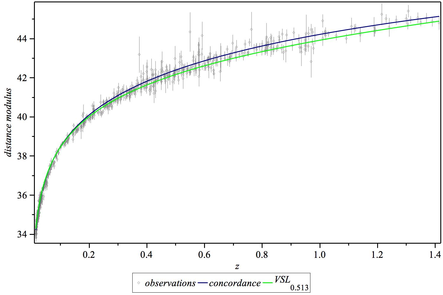
Figure 1: Distance modulus for i) union 2.1 data set [24] ii) concordance model iii) VSL model with $\gamma=0.513$.

As shown in equation (13), $c_{ST}$  varies with redshift for the best fit of $\gamma$. This is shown in Figure 2 .

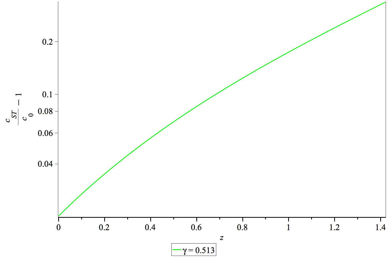
Figure 2: $c_{ST}$  variations vs. redshift for $\gamma=0.513$.

6 Summary and conclusions

In this work we have retaken the debate on the different manifestations of the speed of light in gravitational scenarios. Considering theories formulated in both the Palatini and metric-affine approaches, where the notion of local inertial frame has some subtleties due to the independence of metric and connection, it is possible to explicitly break some of the known degeneracies. In particular, we have pointed out that for the determination of distance, which needs both measuring time and a signal going from one point to another, it is important to distinguish between $c_{ST}$ and $c_{EM}$.

Focusing on the definition of $c_{ST}$, one finds that in the case of $f(\mathcal{R})$ theories $c_{ST}$ is insensitive to the form of the function $f_{\mathcal{R}}(T)$ because the two metrics are conformally related. In other Palatini theories, such as in the case of quadratic gravity, $\mathcal{R}+\alpha\mathcal{R}^{2}+\beta\mathcal{R}_{\mu\nu}\mathcal{R}^{\mu\nu}$, or in Born-Infeld inspired gravity models, $c_{ST}$ may vary in the local frame due to effects of the local stress-energy density which manifest in a non-conformal way. For inverse curvature models, this local density dependence is known to have a nontrivial impact in microscopic systems due to violations of the equivalence principle [16, 17].

Due to the fact that measured distance is not a gauge covariant quantity, the definition of the distance modulus in cosmology is sensitive to the variation of $c_{ST}$ . We have discussed how this quantity should be defined in the varying speed of light case [see Eq.(23)], and have used that definition and the usual one to confront a certain quadratic gravity toy model with supernovae data. The results appear in Sec. 5.1.

The numerical results indicate that the obtained $\chi^{2}_{CM}$ (for $\Lambda$CDM) is comparable with $\chi^{2}_{min,VSL}$ and $\chi^{2}_{min,MEdS}$. However, the MEdS model is inconsistent with Planck data, [23], within the $68\%$ confidence level. So due to the statistical results on the MEdS model, we conclude that the local frame in which the affine connection vanishes is observationally preferred. Although according to the data, $\Lambda$CDM is statistically preferred over the VSL model, it should be noted that the $\Lambda$CDM model involves the ad hoc introduction of a cosmological constant term (of unknown origin) which dominates the energy density of the universe, whereas the VSL model simply assumes a quadratic curvature correction, which could be accommodated within an effective field theory approach. Extension of the analysis presented here to more general gravity Lagrangians will be the subject of future work.

A comment regarding the effective nature of the model (26) and the unusual magnitude of the coupling constant $\Gamma$ considered here is in order. The relation between Palatini geometry and condensed matter physics presented in [25] indicates that in a gravitational context the matter fields can be seen as the analogous of structural defects in crystals. As a result, the effective description of matter at different scales necessarily leads to different types of structural defects, which could imply a dependence of the resulting effective dynamics on the scale. Since different defects in different crystals lead to different properties (such as elasticity, plasticity, conductivity, …) it is legitimate to admit the possibility that the gravitational dynamics governing microscopic scales could be very different from that governing larger scales simply because the structural defects (or, equivalently, the effective matter fields) proper of a scale might be completely different from those present at other scales. The kind of effective geometry (or crystal) corresponding to a certain scale (such as an atom or the solar system, where empty space dominates the total volume) could thus be very different from that corresponding to cosmological models, where a continuous fluid distribution fills all the space. Note, in this sense, that the precise averaging procedure to go from local scales to cosmology is not well understood in GR, let alone in the class of theories considered here, where the connection induces additional nonlinearities in the matter sector. Therefore, the fact that the quadratic model considered in this paper requires a coupling constant $F$ of an unusual magnitude does not necessarily imply that the model could be in conflict with local gravity experiments, where a much smaller coupling constant would be expected. In our view, at those scales the corresponding effective theory of gravity could be very different from that applicable to cosmic scales. For that reason, the viability of this model should be assessed only through its implications at the cosmological level.

Summarizing, though the statistical analysis somehow favors the $\Lambda$CDM model, from a theoretical perspective the quadratic gravity approach is more appealing. Due to the small difference between the $\chi^{2}$ of the concordance and the VSL model, it is not justified to observationally favor one model over the other. Since VSL models can affect the scenario of generating primordial perturbations and structure growth, it is important to study their compatibility with CMB and LSS observations (for more details see [26, 27, 28, 29]). Further research aimed at testing the VSL model with those and other observations is currently underway.

References

- [1] A.G. Riess, A.V. Filippenko, P. Challis, A. Clocchiatti, A. Diercks, P.M. Garnavich, R.L. Gilliland, C.J. Hogan, S. Jha, R.P. Kirshner, B. Leibundgut, M.M. Phillips, D. Reiss, B.P. Schmidt, R.A. Schommer, R.C. Smith, J. Spyromilio, C. Stubbs, N.B. Suntzeff, J. Tonry, The Astronomical Journal 116, 1009 (1998). DOI 10.1086/300499
- [2] S. Perlmutter, G. Aldering, G. Goldhaber, R.A. Knop, P. Nugent, P.G. Castro, S. Deustua, S. Fabbro, A. Goobar, D.E. Groom, I.M. Hook, A.G. Kim, M.Y. Kim, J.C. Lee, N.J. Nunes, R. Pain, C.R. Pennypacker, R. Quimby, C. Lidman, R.S. Ellis, M. Irwin, R.G. McMahon, P. Ruiz-Lapuente, N. Walton, B. Schaefer, B.J. Boyle, A.V. Filippenko, T. Matheson, A.S. Fruchter, N. Panagia, H.J.M. Newberg, W.J. Couch, T.S.C. Project, Astrophysical Journal517, 565 (1999). DOI 10.1086/307221
- [3] L. Amendola, S. Tsujikawa, Dark Energy: Theory and Observations (2010)
- [4] M. Bastero-Gil, M. Borunda, B. Janssen, in American Institute of Physics Conference Series, American Institute of Physics Conference Series, vol. 1122, ed. by K.E. Kunze, M. Mars, M.A. Vázquez-Mozo (2009), American Institute of Physics Conference Series, vol. 1122, pp. 189–192. DOI 10.1063/1.3141250
- [5] J.P. Uzan, in Phi in the Sky: The Quest for Cosmological Scalar Fields, American Institute of Physics Conference Series, vol. 736, ed. by C.J.A.P. Martins, P.P. Avelino, M.S. Costa, K. Mack, M.F. Mota, M. Parry (2004), American Institute of Physics Conference Series, vol. 736, pp. 3–20. DOI 10.1063/1.1835171
- [6] G.J. Olmo, International Journal of Modern Physics D 20, 413 (2011). DOI 10.1142/S0218271811018925
- [7] T.P. Sotiriou, V. Faraoni, Reviews of Modern Physics 82, 451 (2010). DOI 10.1103/RevModPhys.82.451
- [8] S. Nojiri, S.D. Odintsov, Physics Reports505, 59 (2011). DOI 10.1016/j.physrep.2011.04.001
- [9] S. Capozziello, T. Harko, T. Koivisto, F. Lobo, G. Olmo, Universe 1, 199 (2015). DOI 10.3390/universe1020199
- [10] G.F.R. Ellis, J.P. Uzan, American Journal of Physics 73, 240 (2005). DOI 10.1119/1.1819929
- [11] J. Beltran Jimenez, L. Heisenberg, G.J. Olmo, JCAP 1506, 026 (2015). DOI 10.1088/1475-7516/2015/06/026
- [12] B.P. Abbott, R. Abbott, T.D. Abbott, M.R. Abernathy, F. Acernese, K. Ackley, C. Adams, T. Adams, P. Addesso, R.X. Adhikari, et al., Physical Review Letters 116(6), 061102 (2016). DOI 10.1103/PhysRevLett.116.061102
- [13] T.E. Collett, D. Bacon, ArXiv e-prints 1602.05882 (2016)
- [14] D. Blas, M.M. Ivanov, I. Sawicki, S. Sibiryakov, ArXiv e-prints 1602.04188 (2016)
- [15] V.I. Afonso, C. Bejarano, B. Jimenez, G.J. Olmo, E. Orazi, ArXiv e-prints 1705.03806 (2017)
- [16] G.J. Olmo, Phys. Rev. D77, 084021 (2008). DOI 10.1103/PhysRevD.77.084021
- [17] G.J. Olmo, Phys. Rev. Lett. 98, 061101 (2007). DOI 10.1103/PhysRevLett.98.061101
- [18] E.E. Flanagan, Phys. Rev. Lett. 92, 071101 (2004). DOI 10.1103/PhysRevLett.92.071101
- [19] A. Izadi, A. Shojai, Classical and Quantum Gravity 26(19), 195006 (2009). DOI 10.1088/0264-9381/26/19/195006
- [20] A. Izadi, A. Shojai, General Relativity and Gravitation 45, 229 (2013). DOI 10.1007/s10714-012-1467-8
- [21] B. Li, J.D. Barrow, D.F. Mota, Physical Review D76(10), 104047 (2007). DOI 10.1103/PhysRevD.76.104047
- [22] P. Coles, F. Lucchin, Cosmology: The Origin and Evolution of Cosmic Structure, Second Edition (2002)
- [23] Planck Collaboration, P.A.R. Ade, et al., Astronomy and Astrophysics580, A22 (2015). DOI 10.1051/0004-6361/201424496
- [24] N. Suzuki, et. al., Astrophysical Journal746, 85 (2012). DOI 10.1088/0004-637X/746/1/85
- [25] F.S.N. Lobo, G.J. Olmo, D. Rubiera-Garcia, Physical Review D91(12), 124001 (2015). DOI 10.1103/PhysRevD.91.124001
- [26] V. Salzano, M.P. Dabrowski, R. Lazkoz, Physical Review Letters 114(10), 101304 (2015). DOI 10.1103/PhysRevLett.114.101304
- [27] V. Salzano, M.P. Dabrowski, R. Lazkoz, Physical Review D93(6), 063521 (2016). DOI 10.1103/PhysRevD.93.063521
- [28] J.W. Moffat, European Physical Journal C 76, 130 (2016). DOI 10.1140/epjc/s10052-016-3971-6
- [29] W. Lin, M. Ishak, Physical Review D94(12), 123011 (2016). DOI 10.1103/PhysRevD.94.123011