Transitional natural convection with conjugate heat transfer
over smooth and rough walls

Abstract

We study turbulent natural convection in enclosures with conjugate heat transfer. The simplest way to increase the heat transfer in this flow is through rough surfaces. In numerical simulations often the constant temperature is assigned at the walls in contact with the fluid, which is unrealistic in laboratory experiments. The DNS (Direct Numerical Simulation), to be of help to experimentalists, should consider the heat conduction in the solid walls together with the turbulent flow between the hot and the cold walls. Here the cold wall, $0.5h$ thick (where $h$ is the channel half-height) is smooth, and the hot wall has two- and three-dimensional elements of thickness $0.2h$ above a solid layer $0.3h$ thick. The independence of the results on the box size has been verified. A bi-periodic domain $4h$ wide allows to have a sufficient resolution with a limited number of grid points. It has been found that, among the different kind of surfaces at a Rayleigh number $Ra\approx 2\cdot 10^{6}$, the one with staggered wedges has the highest heat transfer. A large number of simulations varying the $Ra$ from $10^{3}$ to $10^{7}$ were performed to find the different ranges of the Nusselt number ($Nu$) relationship as a function of $Ra$. Flow visualizations allow to explain the differences in the $Nu(Ra)$ relationship. Two values of the thermal conductivity were chosen, one corresponding to copper and the other ten times higher. It has been found that the Nusselt number behaves as $Nu=\alpha Ra^{\gamma}$, with $\alpha$ and $\gamma$ independent on the solid conductivity, and dependent on the roughness shape.

I Introduction

Rayleigh-Benard convection is the basic flow to understand several phenomena occurring in nature and in technological applications. This flow has been largely studied theoretically, experimentally and numerically. It is impossible to reference the large number of research papers, these can be found in the review papers by Chillà and Schumacher (2012) and by Lohse and Xia (2010). Before dealing with turbulent flows it is worth understanding the transition from a laminar conducting condition with constant layers of temperature parallel to the cold and hot walls, to a condition where the mutual interaction between temperature and velocity fields generates complex flow structures. In practical applications the solid walls are thick and made of materials with thermal conductivity depending on the applications of interest (Bergman et al., 2011). At low conductivity, the temperature decreases considerably in the solid, while at high conductivity a mild decrease of the temperature in the solid is followed by a large reduction in the fluid. In laminar flows the linear profiles of temperature in the solid and in the fluid have slopes linked to the thermal diffusivity of the solid and of the fluid. This condition is desired in the insulation of buildings, in particular for those covered by glass surfaces. A thin gap between the two glass layers prevent any motion of the air.

In other circumstances the increase of the heat transfer is desired, therefore, once the solid material has been chosen, the heat transfer can be controlled by acting on the shape of the surface between solid and fluid or by letting the fluid to move inside the gap. In both ways changes on the flow structures are promoted. The different shapes of the thermal and flow structures reported in the review paper by Bodenschatz et al. (2000) suggest that, in the presence of smooth walls, for a box with large aspect ratio $\Gamma=l/H$ ($H$ is the gap thickness and $l$ the lateral dimensions of the plates) the first transition generates longitudinal rollers. The transitional Rayleigh number ($Ra=g\alpha\Delta TH^{3}/k\nu$) in the experiments agrees with the value ${Ra_{c}}=1707$ found theoretically by Chandrasekhar (1961). In the expression of $Ra$ $\nu$ is the kinematic viscosity, $k$ the thermal diffusivity of the fluid, $g$ the gravity acceleration, $\alpha$ the thermal expansion coefficient and $\Delta T$ the temperature differences of the two surfaces in contact with the fluid separated by the distance $H$. The spanwise size of the rollers is about $2H$, suggesting that in direct numerical simulations (DNS) in order to capture one convective cell the box size should have at least an aspect ratio $\Gamma=2$. In these circumstances the DNS require limited computational resources to have the sufficient resolution to reproduce the transition from a laminar to an unsteady or to a fully turbulent regime. However it is necessary to demonstrate that the flow structures for $Ra>Ra_{c}$ do not vary with $\Gamma$, and that in fully turbulent conditions ($Ra>>Ra_{c}$), the flow statistics are not affected.

In the fully turbulent regime theoretical and experimental results found that the Nusselt number should vary as $Nu=Q/(k\Delta T/H)\approx Ra^{n}$ ($Q$ is the total heat flux), with the exponent $n$ varying with the Rayleigh number. The present study is focused on the transitional and on the first part of the fully turbulent regime, that is for $Ra_{c}<Ra<10^{6}$. For smooth walls Chandrasekhar (1961) reported the data of Silveston’s experiment (Silveston, 1958), confirming the agreement between the experimental transitional Rayleigh and the theoretical $Ra_{c}=1707$ value. This value was found for rigid boundaries, corresponding to the most unstable wave length $a=3.117H$. By increasing the Rayleigh number, $Nu$ was found to grow as $1+(Ra-Ra_{c})/Ra_{c})^{1/2}$. In Chandrasekhar’s book pictures of the convective cells were also shown, these, being generated between two large circular plates were affected by the side walls. However, it was clear that the width of the cell was about twice the dept of the layer. The picture of the cells reported in figure 15 of Chandrasekhar’s book were not so clear as those given by in figure 5 of Bodenschatz et al. (2000), where the straight rolls at a certain value of $\epsilon=(Ra-Ra_{c})/Ra_{c}$ showed a further instability of wave length smaller than the size of the cell.

From these papers dealing with smooth walls it was clear the mechanism of multiple instabilities leading to a fully turbulent state. Much less is known in the presence of rough surfaces. Numerical simulations in two spatial dimensions (Shishkina and Wagner, 2011) and in a cylindrical container (Stringano et al., 2006) in cylindrical container did not fully clarify the effects of the shape of the roughness surfaces on the flow structures. In fact they did not consider surfaces of different shapes. In numerical and laboratory experiments flow visualization can provide insight on the dependence of the flow structures on the shape of the surface. In real experiments the visualizations require particular care, especially near solid walls. In numerical experiments instead any quantity can be easily visualized and the relative statistics can be calculated. From previous studies it was found a strong flow anisotropy near the surface which reduces moving towards the centre of the container. Temperature and velocity spectra may provide insight on the flow anisotropy, in different regions of the container. In cylindrical containers, frequency spectra do not allow to have a direct link with the flow structures, although these were used by Verzicco and Camussi (1999) to compare their results with those in the experiments. This was emphasized in the review article of Kadanoff (2001) on the structures and scaling in turbulent heat flows. On the other hand, one-dimensional longitudinal and transverse spectra can be calculated at different distances from the walls by using a computational box with two periodic directions. The global effect of the shape of the surface should affect the $Nu(Ra)$ relationship. Roche et al. (2001) observed the ultimate regime ($Nu\approx Ra^{1/2}$) for $Ra>10^{12}$ by inserting a $V$-shaped surface in a cylindrical container. So far, this regime has never been clearly observed in the presence of smooth walls. Du and Tong (2000) compared the $Nu(Ra)$ behavior in a cylindrical cell in the presence of smooth and rough surfaces, and for $10^{9}<Ra<10^{11}$ they observed the same $Nu\approx Ra^{2/7}$ law, however with an increase of more than $76\%$ in the presence of rough walls. Through flow visualizations they found that the dynamics of the thermal plumes over rough surfaces is different from that near smooth surfaces. Stringano et al. (2006) performed numerical simulations for a set-up very similar to that used by Du and Tong (2000), and observed a different $Nu=cRa^{n}$ relationship for smooth and rough surfaces. In particular, for $Ra<10^{7}$ they observed the same behavior for smooth and grooved walls, whereas at higher $Ra$ a steeper growth (with $n=0.37$) was observed for rough walls than for smooth walls (having $n=0.31$). Flow visualizations near the rough surfaces confirmed a plume dynamics similar to that of Du and Tong (2000). Ciliberto and Laroche (1999) considered a rectangular contained with copper walls covered with glass spheres, and obtained the same value of $n$ as for smooth copper plates, but smaller multiplicative constant $c$. The reason should be related to the insulating material of the roughness elements. From these results and from figure 1 of Stringano et al. (2006) it is clear that more investigations are necessary to better understand the influence of the shape and of the material of rough surfaces.

The present study is limited to the transitional regime. Numerical simulations have been performed in a box with two homogeneous directions in order to have the spectra which together with flow visualizations allow to get a clear picture of the flow and thermal structures. The study has been extended to flows with the hot wall corrugated by two- and three-dimensional elements. For this purpose an efficient numerical method to reproduce flows past complex geometries has been used. This tool allows to understand the complex flow physics in the presence of rough walls through the evaluation of any flow quantity. The numerical method developed by Orlandi and Leonardi (2006) has been validated by comparing the results with those obtained by Burattini et al. (2008) in experiments designed to reproduce the numerical simulations. The numerical and laboratory experiments considered turbulent flows in channels with one rough wall with two-dimensional transverse square bars with different values of $w/k$ ($w$ is the separation distance between square bars with height $k$) and different values of the Reynolds number. The method has been extended to simulate conjugate heat transfer including the heat diffusion in the solid layer with smooth and rough walls Orlandi etal 2005 and Orlandi et al. (2016). At high Reynolds numbers part of the viscous, together with the non-linear terms, can be treated explicitly to save computational time. At low $Re$ numbers the viscous restriction $\Delta t/(Re\Delta x^{2})<1/2$ is penalising the efficiency of the simulation, therefore the implicit treatment of the viscous terms is mandatory. However, at low $Re$ coarse grids can be used. Dealing with complex surfaces the resolution is dictated by the requirement to resolve the wall corrugation with a sufficient number of points.

II Physical model and numerical method

II.1 Governing equations

The momentum and continuity equations for the perturbation velocity components and temperature for incompressible flows and within the Boussinesq approximation, are reported by Chillà and Schumacher (2012)

$$\frac{\partial U_{i}}{\partial t}+\frac{\partial U_{i}U_{j}}{\partial x_{j}}=-\frac{1}{\rho_{0}}\frac{\partial P}{\partial x_{i}}+\nu\frac{\partial^{2}U_{i}}{\partial x_{j}^{2}}+g\alpha(T-T_{ref})\delta_{i2};\ \ \ \ \ \ \ \ \ \frac{\partial U_{j}}{\partial x_{j}}=0,$$ (1)

where $U_{i}$ are the components of the velocity vector in the $i$ directions, $p$ is the pressure variations about the hydrostatic equilibrium profile, $x_{1}$, $x_{2}$ and $x_{3}$ are the streamwise, wall-normal and spanwise directions respectively, $\rho_{0}$ is the reference density determined by $-\partial\rho_{0}/\partial x_{2}+\rho_{0}g=0$, $g$ the gravity acceleration, $\nu$ the kinematic viscosity, $\alpha$ the isobaric thermal expansion coefficient, and $T$ the total temperature which is obtained by

$$\frac{\partial T}{\partial t}+\frac{\partial TU_{j}}{\partial x_{j}}=\frac{\partial}{\partial x_{j}}\kappa_{M}\frac{\partial T}{\partial x_{j}}\$$ (2)

here $\kappa_{M}$ is the thermal diffusivity. In this study not only the fluid is considered but also the solid, therefore $\kappa_{M}$ can be either the fluid thermal diffusivity $\kappa_{F}=k/(\rho_{0}C_{p})$, or the thermal diffusivity of the material used for the solid walls, say $\kappa_{S}$. Dimensionless variables are used by introducing as reference quantities the distance between the upper smooth wall and the center of the box $h$, the free-fall velocity $U_{f}=\sqrt{g\alpha\Delta Th}$, and the reference pressure $\rho_{0}U_{f}^{2}$. By introducing the dimensionless temperature $\theta=(T-T_{ref})/\Delta T$ the governing equations become

$$\frac{\partial u_{i}}{\partial t}+\frac{\partial u_{i}u_{j}}{\partial x_{j}}=-\frac{\partial p}{\partial x_{i}}+\frac{1}{Re}\frac{\partial^{2}u_{i}}{\partial x_{j}^{2}}+\theta\delta_{i2};\ \ \ \ \ \ \ \ \ \frac{\partial u_{j}}{\partial x_{j}}=0,$$ (3)

$$\frac{\partial\theta}{\partial t}+\frac{\partial\theta u_{j}}{\partial x_{j}}=\frac{\partial}{\partial x_{j}}\frac{1}{RePr_{M}}\frac{\partial\theta}{\partial x_{j}}\$$ (4)

where $Re=hU_{f}/\nu$, and $2\Delta T$ is the assigned temperature difference between the outer boundary of the lower hot wall and of the upper cold wall, respectively at $x_{2}=1.5h$ and at $x_{2}=-1.5h$. The Reynolds number is linked to the Rayleigh number through the relation $Ra=Re^{2}$ only for perfectly conducting walls or with zero thickness. In the region with the fluid $Pr_{M}=Pr_{F}=1$ has been assumed. For the materials of the solid two different values of $Pr_{M}=Pr_{S}=\kappa_{S}/\kappa_{F}$ have been set, one for the copper $Pr_{S}=0.134$ and the other for a material ten times more conductive, with $Pr_{S}=0.0134$. In the case of smooth walls and for the surface covered by wedges, simulations have also been performed with low conductivity materials $Pr_{S}=1.34$. The total heat flux $Q$ (which is constant along the $x_{2}$ direction) is given by the sum of the turbulent $Q_{T}=<u_{2}\theta^{\prime}>$ and the conductive contribution $Q_{F}=\frac{1}{RePr_{M}}\frac{\partial<\theta>}{\partial x_{2}}$. In the present condition $Q$ is also equal to $Q_{F}=\frac{1}{RePr_{S}}\frac{\partial<\theta>}{\partial x_{2}}$ evaluated in the thick upper solid wall. The overall physical box has dimensions $L_{1}=4h,L_{2}=3h$ and $L_{3}=4h$. The upper (smooth) smooth wall is at $x_{2}=h$, overlaid by a layer of material with thickness $0.5h$. The lower wall is rough, with the plane of crests at $x_{2}=-h$, the roughness thickness is $0.2h$, with a further layer of material underneath with thickness $0.3h$.

At $t=0$, the non-dimensional temperature $\theta$ has been set equal to $\pm 1$ in the two solid layers from $x_{2}=\pm 1.5$ to $x_{2}=\pm 1.$. In the fluid layer the profile of $\theta$ is linear. Random disturbances have been assigned to the velocity field with amplitude equal to $0.02U_{f}$. After a certain time, depending on $Re$, the disturbances may grow or decrease. For laminar flows a large-scale cell forms, and the amplitude of the velocity fluctuations tends to zero. In the transitional regime, after a transient when the initial random fluctuations as well as the $rms$ values decrease, the fluctuations grow exponentially for a short time lapse. The transitional Reynolds number is evaluated by extrapolating to zero the values of the growth rate at different $Re$.

The aspect ratio in the homogeneous directions can affect the results. Kerr (1996), in a range of $Ra$ number similar to that here considered used a domain $L=L_{1}=L_{3}=12h$, wider than used here. This aspect ratio in the presence of roughness elements should require too many grid points, if at least $10$ points are used to represent the surface of each element. The present simulations are devoted to investigating how the shape of the heated rough surface changes the heat transfer, the velocity and temperature structures with respect to those generated by smooth walls. Therefore, it is mandatory to prove that for smooth walls the results of simulations in a wider domain do not change with respect to those performed in the square domain of size $L=4h$.

The system of equations (3), (4) with periodic conditions in the direction $x_{1}$ and $x_{3}$ have been discretized by a finite difference scheme combined with the immersed boundary technique described by Orlandi et al. (2016). The equations were integrated in time with a third-order Runge Kutta low-storage scheme for the explicit nonlinear terms. In the previous simulations an implicit Crank Nicholson procedure based on a factorization of the wide banded matrices was used. For parallel implementation the computational box was subdivided in layers parallel to the walls by limiting the use of a large number of processors. On the other hand, by subdividing the domain in rectangular pencils a greater number of processors can be used. When the factorization is applied the CPU time necessary to transfer data among the processors increases. The implicit treatment of the viscous terms is required at low $Re$ to avoid the viscous stability condition $\Delta t/(Re\Delta x^{2})<2$, which is more restrictive than the Courant-Friedrichs-Lewy (CFL) restriction $|U_{i}\Delta t/\Delta x_{i}|<1$. However, at low $Re$, a coarse grid reduces the amount of data transfer among the processors. At high $Re$, a fine grid is necessary to resolve all the scales and the computational time is kept reasonable by using an explicit scheme for the viscous terms in the momentum equations. For the $\theta$ equation the viscous terms in the homogeneous directions are handled explicitly. Instead the term in the $x_{2}$ direction, due to the large variations of the temperature gradients at the solid/fluid interface, is handled implicitly.

The assumption of a cold wall at the top generates a heat flux from the rough to the smooth wall. Equation (4) holds in the region with the fluid and does not require any condition at the interface between the fluid and the solid because it is solved together with the transport equation for $\theta$ in the solid layers. In these layers $u_{j}=0$, and only the temperature equation is solved, with $Pr_{M}=Pr_{S}$. At the interface the heat flux in the fluid and in the solid sides must be equal; to reach this goal it is convenient to define the $\theta$ at the same location of $u_{2}$ and the diffusivity at the centre of the cell. To account for the difference between fluid and solid a function $f(x_{2})$ is used equal to $1$ in the solid and to $0$ in the fluid. The convective term and $Pr_{F}$ are then multiplied by $(1-f(x_{2}))$ and $Pr_{S}$ by $f(x_{2})$, and the transport equation for $\theta$ becomes

$$\frac{\partial\theta}{\partial t}+(1-f)\frac{\partial\theta U_{j}}{\partial x_{j}}=\frac{\partial}{\partial x_{j}}\frac{1}{Re\;(Pr_{F}(1-f)+Pr_{S}f)}\frac{\partial\theta}{\partial x_{j}}$$ (5)

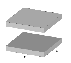
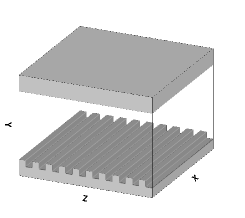
(a) (b) (c)
(d) (e) (f)

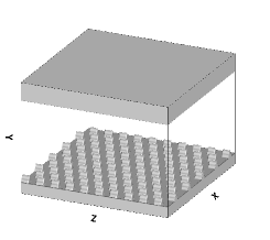
Figure 1: Computational domain for flow over smooth walls SM (a), longitudinal squares bars LSB (b), longitudinal triangular bars LTB (c), transversal triangular bars TTB (d), staggered cubes bars CS (e), and staggered wedges WS (f). The grey shades denote the solid material.

The resolution depends on the Reynolds number. At intermediate values of $Re$ ($Re>75$) the computational grid is $320\times 256\times 320$ points in $x_{1}$, $x_{2}$, $x_{3}$ respectively. The mesh is uniform in the horizontal directions, and non-uniform in the $x_{2}$ direction to increase the resolution at the interface between solid and fluid. For each of the solid layers $32$ grid points were used, and among them $20$ were allocated for the roughness layer. The shape of the roughness elements in the $x_{1}$ and $x_{3}$ directions is reproduced by $16$ grid points. Two-dimensional roughness elements with different orientation as well as three-dimensional elements have been considered to investigate the influence of the shape of the roughness on the heat transfer. The different geometries are indicated as follows (also see figure 1): $LSB$ for square bars with $w/b=1$ oriented along the $x_{1}$ direction, $LTB$ for triangular bars with $w/b=0$ parallel to $x_{1}$, $TTB$ for bars of same shape oriented along the $x_{3}$, $CS$ for staggered cubes with ratio $R_{A}=A_{S}/A_{F}=2$, where $A_{S}=b^{2}$ is the solid area and $A_{F}$ is the fluid area, and $WS$ for a geometry with the same layout, with cubes replaced by wedges. The results are compared with those obtained with two smooth walls, and indicated with $SM$. For the $SM$ and the $WS$ geometry the simulations were performed in a large range of Reynolds number to investigate the $Nu(Ra)$ dependence in the laminar, transitional and fully turbulent regime.

In the present simulations with a strong coupling of the thermal field in the solid and in the fluid layers, the relationship between $Re$ and $Ra$ is not unique. Hence, to compare the results with those in literature it is necessary to relate the Rayleigh number to the Reynolds number in the momentum transport equation. In the present work we select as the relevant temperature difference $\Delta\theta_{F}=<\theta>_{R}-<\theta>_{S}$, with $<\theta>_{R}$ and $<\theta>_{S}$ respectively the mean temperature at the plane of the crest of the roughness elements, and at the top wall. Defining the relevant Rayleigh number as $Ra=g\alpha\Delta T_{F}(2h)^{3}/k\nu$, we get $Ra=4Re^{2}/\Delta\theta_{F}$. The Nusselt number is also defined as $Nu=Q/(\Delta\theta_{F}/(RePr_{F}))$. These expressions point out that in the present simulations $Ra$ can not be fixed a priori, but rather is an output of the simulations, also depending on $Re$ and $Pr_{S}$.

III Results

Large effort was directed numerically, theoretically and experimentally to determine the $Nu(Ra)$ relationship for smooth surfaces. However, much less effort has been put into looking at their dependence in the presence of rough surfaces. Before investigating the effects of the roughness on the $Nu(Ra)$ relationship in the transitional regime, is worth demonstrating the independence of the statistics on the size of the computational box. As previously mentioned, if an influence occurs, it should be more appreciable for smooth walls.

III.1 Domain dependence

$L/h$	$N_{1}\times N_{2}\times N_{3}$	$Ra$	$Nu$	$q_{1}$	$q_{2}$	$q_{3}$	$T_{\theta}$
4	$200\times 128\times 200$	0.51588E+08	0.26712E+02	0.24338E-01	0.50116E-01	0.40605E-01	0.37564E-02
4	$320\times 256\times 320$	0.51672E+08	0.26610E+02	0.24415E-01	0.54737E-01	0.46763E-01	0.39403E-02
8	$640\times 256\times 640$	0.52150E+08	0.25694E+02	0.24080E-01	0.57262E-01	0.55241E-01	0.39125E-02

Table 1: Grid and box sensitivity study: computational parameters and main results. All simulation are carried out for smooth walls, with $Re=3000$, $Pr_{S}=0.134$.

To investigate whether the assumption of a box size with lateral dimensions $L=L_{1}=L_{3}=4h$ is satisfactory to get good results the check has been performed at a value of $Re=3000$, with solid layers made of copper ($Pr_{S}=0.134$). At this Reynolds number the effects of the thermal plumes coexist with those of the large-scale rollers, the former being linked to the resolution, and the latter to the size of the domain. The check consists in the comparison among the results of a simulation with $320\times 256\times 320$ grid points and $L=4h$ and those obtained with the same resolution in a domain with $L=8h$. To check the adequacy of the resolution a further simulation with $L=4h$ and a $200\times 128\times 200$ was performed. The results of the latter have been used to compare the spectra and the profiles of the $u_{2}$ and $\theta$ variances. Flow visualizations of the fluctuations of the same variables are shown at the same distances from the wall where the spectra are calculated. Near the wall the thermal plumes should affect the spectra and the visualizations. The rollers should be better visualised at the center. The simulations were initiated with random disturbances in the velocity components, and it was observed that the rollers may change their orientation during the time evolution.

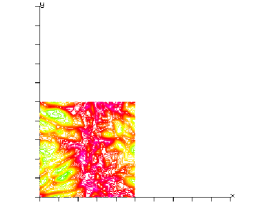
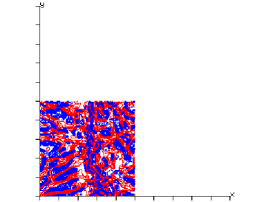
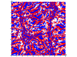
a)                                      b)                                      c)                                      d)

Figure 2: Visualizations of $\theta$ (a,c) and $u_{2}$ (b,d), for $Re=3000$ and $Pr_{S}=0.134$ at $x_{2}=-0.9992$, for box size $L=4h$ (a,b), and $L=8h$ (c,d). Contour levels are given in intervals $\Delta u_{2}=0.001$ (blue negative, red positive), $\Delta\theta=0.01$ from $\theta=0$ and colours from blue to red.

The global results given in table 1 show a difference of $4\%$ between $Nu$ and $Ra$ in large and small boxes. In addition, the results do not differ by changing the resolution, with the meaning that all the flow scales are well resolved also in the coarse simulation. This is better proved by looking at the spectra in Kolmogorov units. Greater but still marginal differences are observed in the values of the integrated variances, $q_{i}=\int<u_{i}^{2}>dx_{2}$, $T_{\theta}=\int<\theta^{\prime 2}>dx_{2}$. The $<\ >$ indicates averages in time and in the two homogeneous directions. The greatest difference in the values of $q_{3}$ are due to the fact that the simulation with $L=8$ hadn’t reached yet a statistically steady state. This comparison was aimed at looking at the instantaneous structures, as shown in figure 2 (near the rough wall) and in figure 3 (at the channel centerline). Figure 2a, indeed shows that one of the two rollers well depicted by $\theta$ contours in figure 2c for the large box, is also captured in the small box. The plumes with red contours of $\theta$ are elongated and correspond to regions of positive $u_{2}$. The elongated plumes which emanate from the interface between the rollers are more clearly visualized by contours of $\theta^{\prime}$ demonstrating that near the wall the contribution $\theta^{\prime}u_{2}$ to the turbulent heat transfer component starts to grow. On the side of these positive thermal plumes there are thermal structures of circular shape due to the descending fluid. Both structures contribute to the component of the turbulent heat flux $Q_{T}=<u_{2}\theta^{\prime}>$. Due to the different evolution the fields at a given time in the small domain cannot exactly reproduce one fourth of the field in the large domain. However, the qualitative comparison between figure 2a and figure 2c, and between figure 2b and figure 2d shows that the flow characteristics near the wall are captured by the simulations in the box of size $4h$. The rollers are well depicted in $x_{1}-x_{3}$ planes at the center of the box, as it is shown in figure 3.

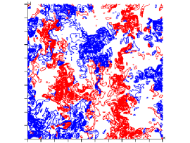
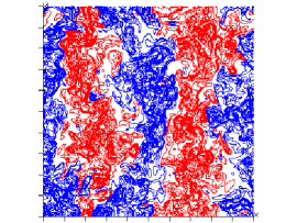
a)                                      b)                                      c)                                      d)

Figure 3: Visualizations of $\theta$ (a,c) and $u_{2}$ (b,d), for $Re=3000$ and $Pr_{S}=0.134$ at $x_{2}=0$, for box size $L=4h$ (a,b), and $L=8h$ (c,d). Contour levels are given in intervals $\Delta u_{2}=0.05$ (blue negative, red positive), $\Delta\theta=0.01$ from $\theta=-.15$ with blue for negative and red for positive.

A proof that the large and the small scales are satisfactorily described by the box with $L=4h$ can be demonstrated by showing the $u_{2}$ and the $\theta$ one-dimensional spectra at the same locations as the visualizations in figure 2 and 3. The calculation of the spectra was done by a large number of fields saved every time unit. To point out the isotropy or anisotropy of the fields at the two different locations the spectra are given in Kolmogorov units, indicated with the superscript $*$. The scaled wavenumber is defined as $k^{*}=k\eta$ with $\eta=(1/(Re^{2}\Omega)^{1/4}$. $\Omega=<\omega_{i}^{2}>$, the scaled velocity spectra are defined as $E^{*}_{{u_{i}}l}=E_{{u_{i}}l}/(\Omega^{2}\eta^{5}/Re^{2})^{1/3}$, and the dimensionless temperature spectra are defined as $E^{*}_{{\theta}l}=E_{{\theta}l}/(\chi(\Omega/Re)^{-1/3}\eta^{5/3})$ with $\chi=\langle(\frac{\partial\theta}{\partial x_{i}})^{2}\rangle$ the rate of temperature dissipation. Near the wall the spectra are expected to be far from isotropic. On the other hand at the channel centerplane ($x_{2}=0$) an isotropic condition should be expected. To investigate whether this is achieved, the velocity spectra are compared with those obtained by Jiménez et al. (1993) and the temperature spectra with the scalar spectra by Donzis et al. (2010). Figure 4a, near the wall, and figure 4b, at the center, show that the velocity and the temperature spectra do not depend on the box size, and, that, in particular, at the intermediate and small scales there is no dependence on the direction. Near the wall $u_{2}$ is very small and increases for the effect of the buoyancy, therefore in figure 4a the amplitude of the $u_{2}$ and the $\theta$ spectra are very different. The magnitude of both the $\theta$ spectra are different from those of forced isotropic turbulence and are greater than both the $u_{2}$ spectra. From the spectra at several distances from the wall, not shown for lack of space, it was observed a rapid tendency to the isotropy. In fact at $x_{2}=0.5$ the spectra are similar to those in figure 4b. A remarkable similarity between the present and the forced isotropic simulations spectra is also obtained in this figure. The same differences between the exponential decay range for the temperature and the $u_{2}$ are reproduced, in particular at the end of the inertial range. This behavior independent on the type of flows indicates that the $\theta$ and $u_{2}$ structures contributing to the terminal part of the inertial range (the so-called bottle-neck) should be very different.

\psfrag{ylab}{$E^{*}_{{\theta}l},\ \ E^{*}_{{u_{2}}l}$}\psfrag{xlab}{$k^{*}$}\includegraphics[width=243.27115pt]{FIG3/fig3a.eps}

\psfrag{ylab}{$E^{*}_{{\theta}l},\ \ E^{*}_{{u_{2}}l}$}\psfrag{xlab}{$k^{*}$}\psfrag{ylab}{$$}\psfrag{xlab}{$k^{*}$}\includegraphics[width=243.27115pt]{FIG3/fig3b.eps}

a)                                                       b)

Figure 4: Flow at $Re=3000$ and $Pr_{S}=0.134$: $u_{2}$ and $\theta$ spectra in the $x_{1}$ direction $l=1$ and in the $x_{3}$ direction at a) $x_{2}=-0.998$ and b) at $x_{2}=0$ compared with the transverse spectra of Jiménez et al. (1993) black and with the scalar spectra by Donzis et al. (2010) blue symbols; the square are $E^{*}_{{u_{2}}1}$ and the circles $E^{*}_{{u_{2}}3}$ the down triangles are $E^{*}_{{\theta}1}$ and the up triangles $E^{*}_{{\theta}3}$. Solid symbols are used for $L=8h$, and open symbols for $L=4h$.

To further demonstrate the independence of the box size, the profiles of the variance of $u_{2}$ and $\theta$ were calculated. In addition to showing that the grid $320\times 256\times 320$ is resolving all the flow scales, the results are compared with those obtained with a grid $200\times 128\times 200$. The good resolution can be further appreciated in figure 4 where the spectra extend up to $k^{*}>2$. Figure 5 shows collapse of the profiles irrespective of the grid and the box size. In this figure the statistics are plotted versus the distance from the walls, therefore the perfect symmetry of the profiles emerges. In addition the large difference in figure 5a between the values of $<u_{2}^{2}>$ and $<\theta^{2}>$ in the near wall region explains why large differences in the spectra at $x_{2}=-0.998$ in figure 4a were observed. The reason of the different behavior between $<\theta^{2}>$ and $<u_{2}^{2}>$ is due to the conductivity of the solid that strictly connect the $\theta$ fluctuations inside the solid to those generated by the turbulent flow motion. In the simulations with isothermal temperature at $x_{2}\pm 1$ $<\theta^{2}>=<u_{2}^{2}>=0$. The profiles in figure 5a accounts for the large scales, as well as the profile of the turbulent kinetic energy $q=<u_{i}^{2}>$ in figure 5b. The satisfactory resolution of the small scales can be appreciated by the profiles of $\Omega$ and $\chi$ which are necessary to evaluate the spectra in Kolmogorov units in figure 4. The relative profiles are shown in figure 5b, which demonstrate that, also in this case there is an independence of the profiles from the resolution and from the size of the computational box. The enstrophy and the rate of temperature dissipation achieve the highest values near the wall and then have a complete different behavior, with $\chi$ nearly constant in the entire domain, while the enstrophy does not largely change near the wall, and decays approximately as $\Omega\approx y^{-1.25}$ within the box.

\psfrag{ylab}{$<u_{2}^{2}>,\ \ <\theta^{2}>$}\psfrag{xlab}{$y/h$}\includegraphics[width=243.27115pt]{FIG4/fig4b.eps}

\psfrag{ylab}{$<u_{2}^{2}>,\ \ <\theta^{2}>$}\psfrag{xlab}{$y/h$}\psfrag{ylab}{$q,\Omega,\chi$}\psfrag{xlab}{$y/h$}\includegraphics[width=243.27115pt]{FIG4/fig4a_pw.eps}

a)                                                       b)

Figure 5: Flow at $Re=3000$ and $Pr_{S}=0.134$. Vertical profiles of: a) $<u_{2}^{2}>$ (red) and $<\theta^{2}>$ (black); b) $q$ (blue), $\Omega$ (red) and $\chi$ (green). Open symbols indicate results obtained with $L=4h$ $320\times 256\times 320$, solid symbols with $L=8h$ $640\times 256\times 640$, and lines with $L=4h$ $200\times 128\times 200$. The dashed line denotes $\approx y^{-1.25}$. The values of the respective Rayleigh numbers are given in table 1.

Having demonstrated that for natural convection in the presence of heat conducting smooth walls at $Re=3000$, when the flow can be considered fully turbulent, the results do not depend on the lateral size of the box, in the next section we investigated the influence of the roughness shape at lower value of the Reynolds number.

III.2 Roughness influence

Geometry	$Ra$	$Nu$	$q_{1}$	$q_{2}$	$q_{3}$	$T_{\theta}$
$SM$	0.22664E+07	0.11389E+02	0.79858E-01	0.11134E+00	0.44864E-01	0.20216E-01
$WS$	0.14870E+07	0.19359E+02	0.76241E-01	0.11775E+00	0.47854E-01	0.23993E-01
$SC$	0.16399E+07	0.17266E+02	0.59798E-01	0.10997E+00	0.56664E-01	0.24381E-01
$LSB$	0.18326E+07	0.15142E+02	0.97332E-01	0.12395E+00	0.38397E-01	0.25379E-01
$LTB$	0.16993E+07	0.15890E+02	0.10787E+00	0.13016E+00	0.33158E-01	0.24042E-01
$TTB$	0.17334E+07	0.15264E+02	0.53122E-01	0.11165E+00	0.63454E-01	0.21516E-01

Table 2: Values of some of the global quantities obtained for numerical simulations over rough walls at $Re=500$,d $Pr_{S}=0.134$.

The global results for the six types of surfaces mentioned above (see figure 1) are given in table 2. The simulations were performed by fixing the Reynolds number $Re=500$ and the solid layer is considered to be made of copper ($Pr_{S}=0.134$). Although $Re$ is fixed, table 2 indicates a large dependence of $Ra$ and $Nu$ on the shape of the surface roughness. In particular, the values of $Nu$ are greater than those obtained by smooth walls, and surfaces with three-dimensional elements lead to higher heat transfer than achieved with two-dimensional bars. As should be expected, the $90^{0}$ change of orientation of bars with the same shape produces values of $Nu$ not too different. The slight increase of $Nu$ obtained for the $LTB$ with respect to the $LSB$ surface implies that the edges of the triangular bars improve the heat transfer. The higher efficiency of the wedges is demonstrated by comparing $Nu$ for the $SC$ and $WS$ surfaces. The influence of the orientation of the two-dimensional elements can be appreciated by comparing the values of $q_{1}$ and $q_{3}$ in table 2.

The qualitative influence of the shape of roughness on the flow structures can be appreciated by surface contours of $u_{2}$ and $\theta^{\prime}$. Three-dimensional plots in the region above the rough surfaces are shown at the values of $Re$ and $Pr_{S}$ reported in the caption of table 2. The surfaces of $\theta^{\prime}=\theta-\overline{\theta}=\pm 0.1$ in figure 6b-f for the five rough surfaces, are compared with those of the smooth wall given in figure 6a. For these visualizations the averages, indicated by an overbar, are performed in the $x_{1}$ and $x_{3}$ homogeneous directions by taking only one field. At $Re=500$ there is a marginal influence of the small scale turbulence on the large scale structures that are mainly related to the shape of the surface.

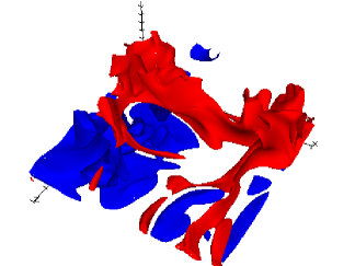
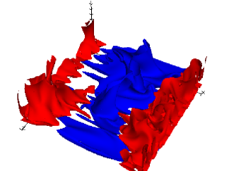
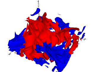
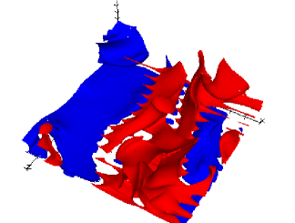
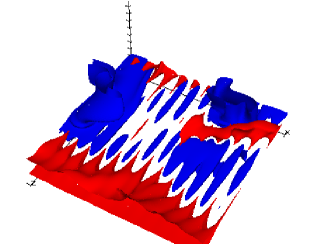
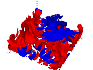
a)                                              b)                                              c)            d)                                              e)                                              f)

Figure 6: Fluctuating $\theta$ surface contours, red $\theta^{\prime}=+0.1$ blue $\theta^{\prime}=-0.1$ above the heated surface at $Re=500$ and $Pr_{S}=0.134$: a) smooth $SM$, b) longitudinal square bars $LSB$, c) three-dimensional staggered cubes $CS$, d) longitudinal triangular bars $LTB$, e) transverse triangular bars $TTB$, f) three-dimensional staggered wedges $WS$.

In figure 6a the rollers for the $SM$ surface, previously described at a higher Reynolds number, are oriented in the $x_{1}$ direction. Some unstable small structures are visible, which at this value of $Re$ have a size comparable to that of the rollers. Longitudinal square bars $LSB$, in figure 6b promote a longitudinal motion within the bars with the effect of orienting the rollers in the $x_{3}$ direction. This effect is corroborated by the orientation induced by the triangular longitudinal bars $LTB$ in figure 6d. The triangular shape of the elements promotes a greater penetration of the hot rollers in the space between the bars, leading to a greater value of $q_{1}$ for $LTB$ than that for $LSB$ in table 2.

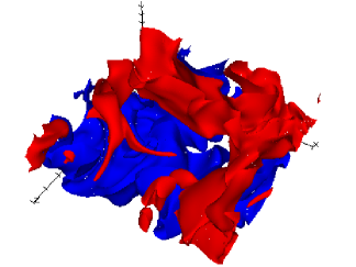
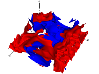
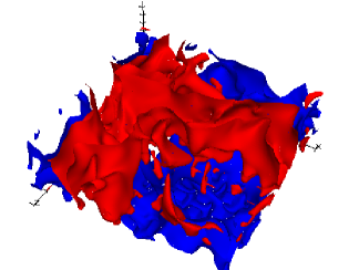
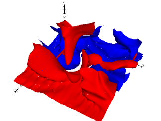
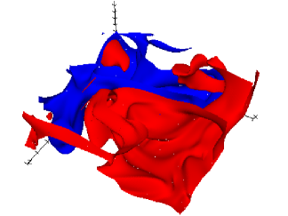
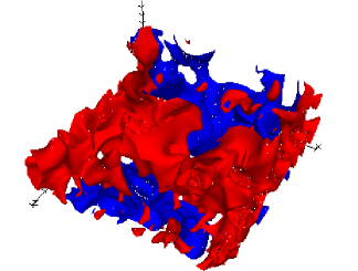
a)                                              b)                                              c)            d)                                              e)                                              f)

Figure 7: Fluctuating $u_{2}$ surface contours, red $u_{2}^{\prime}=+0.1$ blue $u_{2}^{\prime}=-0.1$ above the heated surface at $Re=500$ and $Pr_{S}=0.134$: a) smooth $SM$, b) longitudinal square bars $LSB$, c) three-dimensional staggered cubes $CS$, d) longitudinal triangular bars $LTB$, e) transverse triangular bars $TTB$, f) three-dimensional staggered wedges $WS$.

These two surfaces produce values of $q_{1}$ greater than those of the other surfaces (see table 2). The influence of the bars orientation on the shape of the structures is depicted by the $90$ degree change of the orientation from $LTB$ (figure 6b). to $TTB$ (figure 6e). Depending on the time chosen for the visualizations of the three-dimensional elements, both for cubes $CS$ (figure 6c) and wedges $WS$ (figure 6f) the rollers can be oriented in different directions.

The surface contours of $u_{2}$ given in figure 7 lead to the same conclusions concerning the orientation of the structures. In addition, comparing figure 6 and 7, the qualitative conclusion of a higher correlation between $u_{2}$ and $\theta^{\prime}$ for the three-dimensional surfaces can be drawn. It seems also that for the other surfaces these two quantities are less correlated. A more quantitative result is obtained by evaluating the correlation coefficient $C_{v\theta}=<u_{2}\theta^{\prime}>/\sqrt{<u_{2}^{2}><\theta^{\prime}2>}$ evaluated over a large number of fields, which is plotted in figure 8c. The values of $C_{v\theta}$ ($C_{v\theta}=0.4$) are low at the plane of the crest for $SM$ and for the geometries with two-dimensional bars. On the other hand $C_{v\theta}$ is more uniform in the near-wall region for walls with three-dimensional roughness, implying that the velocity fluctuations begin to be linked to the thermal fluctuations in the region within the solid elements. The $C_{v\theta}$ correlations grow in the region above the surface and reach their maximum at the location where the production of $<\theta^{\prime 2}>$ ($<u_{2}\theta^{\prime}>\frac{\partial<\theta>}{\partial x_{2}}$ has a maximum. This point is located within the thermal boundary layer, which is however only well defined for smooth surfaces.

Profiles of the vertical velocity variance $v_{2}=<u_{2}^{2}>^{1/2}$ and of the temperature variance $T^{\prime}=<\theta^{\prime 2}>^{1/2}$ obtained by averaging in the homogeneous direction and in time show a different trend near rough surfaces. The $v_{2}^{2}$ start from different values at the plane of the crest (figure 8a), depending on the shape of the hot surfaces, and reach the highest value at the center (figure 8a). As expected, three-dimensional roughness produces stronger values of $v_{2}$ at the plane of the crests than those generated by two-dimensional roughness. The main effect of the $u_{2}$ disturbances at the plane of the crest is to promote a growth of $v_{2}$ proportional to $y$ ($y=1-|x_{2}|$ for $|x_{2}|<1$), namely the distance from the surface. In the near-wall region of the smooth surfaces instead it has been observed that $v_{2}\approx y^{2}$, as shown in the inset of figure 8a, where the lines are evaluated in the region near the smooth upper wall. The temperature variances $T^{\prime}$ depicted in figure 8b have a rather complex behavior inside the roughness layer and near the plane of the crests ($x_{2}=-1$). The differences among the values of $T^{\prime}$ for $x_{2}<-1.2$ implies that the flow within the elements and the shape of the solid elements do affect the thermal field in the solid layer on which the elements are mounted. Due to the enhancement of the lateral heat transfer within the three-dimensional elements the maximum of $T^{\prime}$ is typically below $x_{2}=-1$. For the two-dimensional surfaces the maximum, above the plane of the crests, moves closer to $x_{2}=-1$ with respect to that of $SM$ located at the location of the maximum production of $<\theta^{\prime 2}>$. This behavior, as mentioned before discussing figure 8a, implies that in the presence of rough surfaces the definition of a thermal boundary layer thickness is no longer appropriate. Figure 8b in addition shows that nearly the same value of $T^{\prime}$ at the center is reached for all geometries.

The strong correlation between $\theta^{\prime}$ and $u_{2}$ producing the prevalence of $Q_{T}$ in the interior of the fluid region can be understood in more detail by looking at figure 6 and figure 7, in which a strong correspondence of red and blue regions of $u_{2}$ and $\theta^{\prime}$ can be appreciated, meaning that the turbulent heat transfer is associated with hot ascending and cold descending plumes. In addition it appears that $u_{2}$ surfaces reproduce rather well the formation and orientation of the large-scale rollers. Qualitatively the strong correlation between $u_{2}$ and $\theta^{\prime}$ more uniformly distributed near the three-dimensional surfaces and extending deeply in the flow helps to understand why the heat transfer is enhanced. The quantitative measure is obtained by the values of the $Nu$ numbers in table 2. The present simulations have demonstrated that the highest heat transfer obtained by three-dimensional wedges is due the formation of strong plumes at the cusp of the solid elements. Therefore it is worth investigating in greater detail the differences between the statistics and the structures generated by the $WS$ surface with respect to those by the smooth wall when $Re$ and $Pr_{S}$ are changed.

\psfrag{ylab}{$<u_{2}^{2}>^{1/2}$}\psfrag{xlab}{$x_{2}$}\includegraphics[width=143.6865pt]{FIG7/fig7a.eps}

\psfrag{ylab}{$<u_{2}^{2}>^{1/2}$}\psfrag{xlab}{$x_{2}$}\psfrag{ylab}{$<\theta^{\prime 2}>^{1/2}$}\psfrag{xlab}{$x_{2}$}\includegraphics[width=143.6865pt]{FIG7/fig7b.eps}

\psfrag{ylab}{$<u_{2}^{2}>^{1/2}$}\psfrag{xlab}{$x_{2}$}\psfrag{ylab}{$<\theta^{\prime 2}>^{1/2}$}\psfrag{xlab}{$x_{2}$}\psfrag{ylab}{$C_{v\theta}$}\psfrag{xlab}{$x_{2}$}\includegraphics[width=143.6865pt]{FIG7/fig7c.eps}

a)                                              b)                                              c)

Figure 8: Profiles of a) vertical velocity variance, b) temperature variance, and c) $v\theta$ correlation coefficient, for different surfaces as indicated by the insets in panels b) and c).

III.3 Transitional regime

III.3.1 Time evolution and visualizations

To investigate the transitional regime simulations at low and intermediate values of the Reynolds number should be performed. At low $Re$ the numerical procedure requires implicit treatment of the viscous terms to avoid the time step restriction $\Delta t/\Delta xRe<2$. The increase of CPU due to the inversion of tridiagonal matrices and to the enhancement of the data transfer among the processor is not so penalising, at low $Re$, because the small velocity and temperature gradients require less resolution.

The experiments of Silveston (1958) confirmed the theoretical value $Ra_{c}=1707$, of the transitional Rayleigh number for smooth walls. In addition, the experiments showed that $Nu$ was growing as $Ra^{n}$, with large variations of $n$ for $1078<Ra<10^{6}$. To investigate whether the present numerical simulations with conducting solid walls reproduce these observations, at $t=0$ a uniform temperature distribution along the $x_{1}$ and $x_{3}$ directions is imposed in the fluid layer with $\frac{\partial\theta}{\partial x_{2}}=1$, and the flow instability is triggered by assigning random velocity disturbances. The time evolution of the integrated velocity disturbances $q_{i}=\int\overline{u_{i}^{2}}^{1/2}dx_{2}$ are analysed in figure 9. Initially, the velocity disturbances decrease due to viscous energy dissipation at the small scales. The large viscosity at low Reynolds number, also dissipates energy at the large scales leading to a laminar state characterised by a linear temperature profile, irrespective of the shape of the surface. For smooth conducting surfaces at $Pr_{S}=0.0134$ (highly conductive material) the temperature at the walls are found to be $\pm 0.993$. For the $WS$ surface we find $\theta_{R}=0.84$ at the plane of the crest, and $\theta_{S}=-0.94$ at the opposite smooth wall. To understand why $|\theta_{R}|<|\theta_{S}|$, for $Ra<Ra_{c}$, it should be recalled that inside the solid elements the temperature decreases less than in the fluid regions surrounding the solid elements, as $Pr_{F}>Pr_{S}$. The different decrease of temperature in the layer with the solid elements produces undulations of $\theta$ in the fluid layer near the plane of the crests, whose amplitude rapidly decreases moving towards the centre. Regarding the flow structures at $Ra<Ra_{c}$, the contours of the velocity components $u_{1}$ and $u_{2}$ show at a certain time the formation of two convective cells whose strength decreases in time in the case of smooth walls. This can be appreciated by the time evolution of $q_{2}$ in figure 9a. For $WS$ the motion within the rough elements does not largely affect the large-scale cells. The three-dimensional velocity and temperature disturbances generated by the $WS$ surfaces are not strong enough to trigger the spanwise motion on the large scale cells. The flow structures occurring in the initial time evolution for $Ra<Ra_{c}$ are not presented, being similar to those at $Re=20$, discussed later on.

\psfrag{ylab}{$q_{2}$}\psfrag{xlab}{$t$}\includegraphics[width=220.50885pt]{FIG8/fig8a.eps}

\psfrag{ylab}{$q_{2}$}\psfrag{xlab}{$t$}\psfrag{ylab}{$q_{3}$}\psfrag{xlab}{$t$}\includegraphics[width=220.50885pt]{FIG8/fig8b.eps}

a)                                                         b)

Figure 9: Time history of integrated squared velocity disturbances: a) $q_{2}$ and b) $q_{3}$ at red $Re=10$, green $Re=12.5$, magenta $Re=20$, cyan $Re=50$, blue $Re=75$, and black $Re=250$; symbols $WS$, lines $SM$.

Figure 9 shows the time history of the $q_{i}$ ($q_{1}$ is not plotted being similar to that of $q_{3}$). The discussion about the large values found for the correlation coefficient $C_{v\theta}$ suggests to get an exponential growth of $q_{\theta}$ close to that of $q_{2}$. Indeed this has been observed with a time behavior for $q_{\theta}$ similar to that in figure 9a. The difference is in the initial evolution because of the absence of $\theta$ fluctuations at $t=0$. At any $Re$ (the corresponding values of $Ra$, at the end of the simulations, are given in the figure caption), the decrease in the short initial period, occurs for the dissipation at different rates of the different scales contributing to $q_{i}$. At $Re=10$, $q_{2}$ in figure 9a reaches a constant level which depends on the shape of the surface. On the other hand, at $Re=12.5$, while $q_{2}$ tends to a constant for $SM$, it grows exponentially for $WS$. This is a first indication that the critical Rayleigh number for $WS$ is smaller than than for smooth wall. In figure 9b it is seen that at $Re<50$, for both geometries $q_{3}$ does not reach values close to $q_{2}$, which is the condition supporting the formation of large amplitude three-dimensional instabilities. For the $WS$ geometry at $Re=12.5$ (green symbols) the value $q_{3}=0.00001$ at $t=100$ accounts for the three-dimensional disturbances within the roughness, which affect a thin layer of fluid near the plane of the crests.

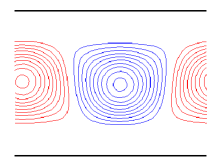
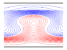
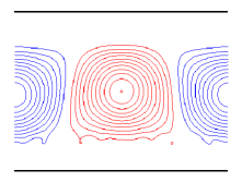
a)                     b)                     c)                     d)

Figure 10: Flow at $Re=20$, $Pr_{S}=0.134$: Contour plots in a $x_{1}-x_{2}$ plane at $x_{3}=2$ of $u_{2}$ (b, d) and of $\theta$ (a, c), for smooth walls (a, b) and for the $WS$ geometry (c, d). Contours are given in intervals $\delta=0.05$, blue negative, red positive.

At $Re=20$ both flows have a similar growth of $q_{2}$ (magenta in figure 9a), and the corresponding flow structures at $t=100$ are depicted in figure 10 trough $\theta$ and $u_{2}$ contour plots in a $x_{1}-x_{2}$ plane at $x_{3}=2$. The temperature distribution inside the solid are better visualized at $Pr_{S}=0.134$ than at $Pr_{S}=0.0134$, where the contours are clustered near the plane of the crests. The $u_{2}$ contours in figure 10b ($SM$) and figure 10d ($WS$) are similar except for a spatial shift. In the latter case the small disturbances emerging from the interior of the rough surface are barely appreciated, and do not affect the contours in the central part of the domain. The strong $\theta$ undulations inside the roughness (figure 10c) do not protrude into the flow, in fact, far from the plane of the crests the contours of $\theta$ in figure 10a are similar to those in figure 10c.

In figure 9a the time history of $q_{2}$ at $Re=20$ (magenta) and $Re=50$ (cyan) for the $SM$ flow are very similar, however the visualizations at $Re=50$ (not shown) show two vertically oriented cells rather than a single cell. The same number of cells also appear for $WS$, with the $u_{2}$ and $\theta$ disturbances due to the three-dimensional surface, as at $Re=20$, localised in a thin layer of fluid near the plane of the crest. This was observed at $t=30$, at the end of the exponential growth.

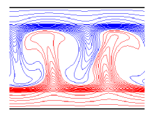
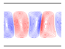
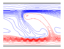
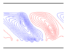
a)                     b)                     c)                     d)

Figure 11: Flow at $Re=75$, $Pr_{S}=0.134$: Contour plots in a $x_{1}-x_{2}$ plane at $x_{3}=2$ of $u_{2}$ (b, d) and of $\theta$ (a, c), for smooth walls (a, b) and for the $WS$ geometry (c, d). Contours are given in intervals $\delta=0.05$, blue negative, red positive.

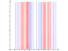
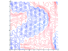
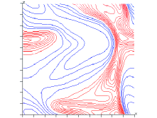
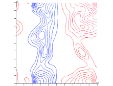
a)                     b)                     c)                     d)

Figure 12: Flow at $Re=75$, $Pr_{S}=0.134$: Contour plots of $\theta^{\prime}$ in a $x_{1}-x_{3}$ plane at $x_{2}=-0.76$ for $SM$ (a) and $WS$ (b), at $x_{2}=-0.99$ for $WS$ (c), and at $x_{2}=0$ for $WS$. Contours are given in intervals $\delta=0.05$, blue negative, red positive.

The undulations of the $q_{i}$, after the exponential growth, in particular in figure 9 are related to the unsteadiness of the structures. In this figure the second growth for $q_{3}$ at $Re=50$ for $WS$ (cyan symbols) is due to the formation of disturbances oriented in the spanwise direction. In figure 9b there is a similarity between the evolution of $q_{3}$ for $Re=75$ (blue symbols) and for $Re=50$; the difference is the time when the fast growth is initiated. The higher amplitudes of $q_{3}$ for $Re=75$ allow better visualizations. Figure 11a and figure 11b indeed shows, for smooth walls, the formation of two slightly inclined cells. The cells oscillate from left to right in time producing the small undulations of the blue line in figure 9a. For this flow the spanwise disturbances (indicated by $q_{3}$) grow for a short time ($8<t<16$) to reach a small value ($q_{3}=0.0001$), and then sharply decrease (blue line in figure 7b). Differently, for the $WS$ flow the spanwise velocity disturbances grow continuously in time, with resulting change in the shape of the main rollers. Figures 11c and figure 11d indeed depict the formation of strong inclined thermal plumes. In these circumstances the flow has a chaotic behavior as emerges from the oscillations in figure 9b, therefore the spanwise disturbances do not have a well defined wavenumber.

Contour plots of $\theta^{\prime}$ in wall-parallel $x_{1}-x_{3}$ planes at different $x_{2}$ locations, better emphasize the shape of the spanwise structures. Indeed the parallel straight lines in figure 12a evaluated at $x_{2}=-0.76$ demonstrate the absence of thin temperature plumes with ordered or disordered for the $SM$ geometry. The visualization at $x_{2}=0$ (not reported) is similar, with the lines shifted to the left or to the right, indicating that the thermal plumes in figure 11a oscillate in the $x_{1}$ direction. On the other hand, the velocity and thermal disturbances generated by the three-dimensional surface affect the shape of the plumes in a complicated way, as shown in figure 12(b,c,d). The interaction between the disturbance of each wedge, at $x_{2}=-0.99$ (figure 12b) causes the bending of the large-scale rollers, and, in certain regions strong temperature gradients are created, with local increase of the heat flux. At $x_{2}=-0.76$ (figure 12c) the effect of the single solid element disappears but the shape of the rollers, and the sharp $\theta^{\prime}$ gradients are still visible. At $x_{2}=0$ (figure 12d) the rollers have wave-like disturbances aligned along the $x_{3}$ direction. Near the smooth top surface, at $x_{2}=0.76$ contours similar to those in figure 12c are obtained with blue and red interchanged, therefore this picture is not shown.

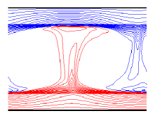
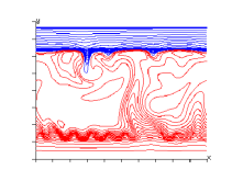
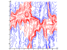
a)                     b)                     c)                     d)

Figure 13: Flow at $Re=250$, $Pr_{S}=0.134$: Contour plots of $\theta^{\prime}$ in a $x_{1}-x_{2}$ plane at $x_{3}=2$ for $SM$ (a) and $WS$ (c), and in a $x_{1}-x_{3}$ plane at $x_{2}=-0.976$ for $SM$ (b) and $WS$ (d). Contours are given in intervals $\delta=0.05$, blue negative, red positive.

At $Re=250$ the $SM$ and the $WS$ surfaces produce only one cell with high temperature gradients near the walls, with that for $SM$, in figure 13a, better defined than than for $WS$ in figure 13c. The visualizations in the $x_{1}-x_{2}$ planes, for the $SM$ surface do not allow to make conjectures on the formation of spanwise disturbances. The formation, growth and persistence of these disturbances is the key process leading to have a fully turbulent regime when the Reynolds number increases. Indeed the appearance of the spanwise disturbances at $Re=250$ for $SM$ could be conjectured based on the time evolution of $q_{3}$ in figure 9b. In fact the black line for $SM$ at $t>30$ was tending to a constant value smaller than for $WS$. To better see the shape of the spanwise disturbances the contours of $\theta$ in $x_{1}-x_{3}$ planes are presented at $x_{2}=-0.76$ in figure 13b for $SM$ and in figure 13d for $WS$. For $SM$ a short wave instability in the $x_{3}$ direction is visible, whereas for $WS$ a more complex thermal structure than previously discussed at $Re=75$ (figure 12c), can be observed at $x_{2}=-0.76$. As in figure 12c, at this distance from the wall, the imprinting of the solid elements is barely appreciated.

As previously shown at $Re=500$ in figure 6 and in figure 7 the shape of $\theta^{\prime}$ surfaces (smoother than that of $u_{2}$) does not largely differ from that of $u_{2}$, and with a correspondence of the negative and of the positive values. At $Re=500$ the surfaces were corrugated implying that flows with a wide range of scales were generated, and the spectra were highlighting the energy and thermal distribution among the scales.

\psfrag{ylab}{$Q_{T},Q_{F}$}\psfrag{xlab}{$x_{2}$}\includegraphics[width=206.28247pt]{FIG13/fig13a.eps}

\psfrag{ylab}{$Q_{T},Q_{F}$}\psfrag{xlab}{$x_{2}$}\psfrag{ylab}{$Nu_{T},Nu_{F}$}\psfrag{xlab}{$x_{2}$}\includegraphics[width=206.28247pt]{FIG13/fig13b.eps}

a)                                                       b) \psfrag{ylab}{$Q_{T},Q_{F}$}\psfrag{xlab}{$x_{2}$}\psfrag{ylab}{$Nu_{T},Nu_{F}$}\psfrag{xlab}{$x_{2}$}\includegraphics[width=120.92421pt]{FIG13/fig13c.eps} \psfrag{ylab}{$Q_{T},Q_{F}$}\psfrag{xlab}{$x_{2}$}\psfrag{ylab}{$Nu_{T},Nu_{F}$}\psfrag{xlab}{$x_{2}$}\includegraphics[width=120.92421pt]{FIG13/fig13d.eps} \psfrag{ylab}{$Q_{T},Q_{F}$}\psfrag{xlab}{$x_{2}$}\psfrag{ylab}{$Nu_{T},Nu_{F}$}\psfrag{xlab}{$x_{2}$}\includegraphics[width=120.92421pt]{FIG13/fig13e.eps} \psfrag{ylab}{$Q_{T},Q_{F}$}\psfrag{xlab}{$x_{2}$}\psfrag{ylab}{$Nu_{T},Nu_{F}$}\psfrag{xlab}{$x_{2}$}\includegraphics[width=120.92421pt]{FIG13/fig13f.eps}    c)                     d)                     e)                     f) \psfrag{ylab}{$Q_{T},Q_{F}$}\psfrag{xlab}{$x_{2}$}\psfrag{ylab}{$Nu_{T},Nu_{F}$}\psfrag{xlab}{$x_{2}$}\includegraphics[width=120.92421pt]{FIG13/fig13g.eps} \psfrag{ylab}{$Q_{T},Q_{F}$}\psfrag{xlab}{$x_{2}$}\psfrag{ylab}{$Nu_{T},Nu_{F}$}\psfrag{xlab}{$x_{2}$}\includegraphics[width=120.92421pt]{FIG13/fig13h.eps} \psfrag{ylab}{$Q_{T},Q_{F}$}\psfrag{xlab}{$x_{2}$}\psfrag{ylab}{$Nu_{T},Nu_{F}$}\psfrag{xlab}{$x_{2}$}\includegraphics[width=120.92421pt]{FIG13/fig13i.eps} \psfrag{ylab}{$Q_{T},Q_{F}$}\psfrag{xlab}{$x_{2}$}\psfrag{ylab}{$Nu_{T},Nu_{F}$}\psfrag{xlab}{$x_{2}$}\includegraphics[width=120.92421pt]{FIG13/fig13j.eps}    g)                     h)                     i)                     j)

Figure 14: Flow at $Re=250$, $Pr_{S}=0.134$: profiles of the heat fluxes $Q_{T}$ and $Q_{F}$ (a) and of their contribution to the Nusselt number (b). The solid symbols denote statistics taken by averaging over one realisation, in the text indicated by $\overline{}$; solid lines denote time averaged. Red stands for $SM$, and black for $WS$. Visualizations through surface contours are shown in panels b-f, for $u_{2}$ (c,g), $\theta^{\prime}$ (d,h), $\frac{1}{Re}\frac{\partial{\theta}}{\partial x_{2}}$ (e,i), ${\theta^{\prime}u_{2}}$ (f,j). Data are shown for $SM$ in (c,d,e,f) and for $WS$ in (g,h,i,j). Blue and red contours correspond to negative red positive values, respectively, with value $\pm 0.1$ (c,d,g,h) and $\pm 0.01$ (e,f,i,j).

From the spectra, not shown here for lack of space, it was possible to see that at this Reynolds number the influence of the shape of the surface was barely detected at the location of maximum production of $<\theta^{\prime 2}>$. In the spectra at $Re=250$ at the centerline there are differences between the $SM$ and the $WS$, that did not appear at $Re=500$. At the higher Reynolds number the one-dimensional spectra of $u_{2}$ and $\theta$ in $x_{1}$ coincided with those in $x_{3}$ at the center. On the other hand, at $Re=250$ in the spectra along $x_{3}$ a clear signature of discrete wavenumber was detected. This occurrence suggests that the well organised structures in figure 13b extend up to the center of the box. Therefore to understand in greater detail, at this Reynolds number, the heat transfer mechanism due to well organised structures for $SM$, and to a wider range of scales for $WS$ a global picture of the quantities contributing to the total heat flux ($Q_{T}$ and $Q_{F}$) are shown.

The visualizations are evaluated with a single field, which approximates within a certain measure the averaged heat transfer. The profiles of the two contributions in figure 14a prove that for $SM$ the approximation is better than that for $WS$ surfaces, implying a stronger dynamics of the turbulent component $\overline{Q_{T}}$ generated by the flow motion within the roughness elements. This difference in fact is not observed in the profiles of $\overline{Q_{T}}$ and $\overline{Q_{F}}$ near the top surface. This figure emphasizes that the averaged heat fluxes for the two surfaces do not largely differ, with the exception of the thin region near the plane of the crests. On the other hand when the respective contributions to the Nusselt number are calculated ($\overline{Nu_{T}}=\overline{Q_{T}}/Q_{K}$ and $Nu_{F}=\overline{Q_{F}}/Q_{K}$ with $Q_{K}=\frac{\overline{\theta_{R}}-\overline{\theta_{S}}}{Re}$) a large difference between the $SM$ and the $WS$ surfaces appears in the central region in figure 14b. This is due to the large differences in the values of $Q_{K}$ for the $SM$ and $WS$ surfaces. From these two figures and in particular from the behavior in the near-wall region of $\overline{Q_{T}}$ and $\overline{Q_{F}}$ it turns out that large differences in the distribution of the two fluxes between the $SM$ and $WS$ surfaces should occur. To explain why this happens, the surface contours of $u_{2}$, $\theta^{\prime}$, $u_{2}\theta^{\prime}$ and $\frac{1}{Re}\frac{\partial{\theta}}{\partial x_{2}}$ in figure 14 are given. The $\theta^{\prime}$ and $u_{2}$ surfaces in figure 14c and figure 14d show that the corrugation in the presence of the smooth surface is regular and it consist on four thermal plumes due to the exponential growth of the secondary instability of the $u_{3}$ disturbances. These disturbances extend in a large region above the wall. The rather good correspondence between red and blue regions of $u_{2}$ and $\theta^{\prime}$ cause the formation of large regions of positive turbulent heat flux$\theta^{\prime}u_{2}$ depicted in figure 14f. The blue regions have a limited extension. Figure 14e shows that the conductive heat flux $\frac{1}{Re}\frac{\partial{\theta}}{\partial x_{2}}$ is localised near the smooth wall, with reduced effect of the spanwise disturbances. The comparison between the profiles of the averaged and the instantaneous contributions emphasizes that at this value of $Re$ in the presence of smooth surfaces the dynamics is rather slow. The visualizations of the same quantities for the $WS$ surfaces, on the other hand, show a thicker layer where the disturbances emanating from the roughness affect the turbulent heat flux. This is particularly evident by the wider and taller red regions in figure 14j with respect to those in figure 14f. The dynamics of this thick layer produces at this time an overshoot of $\overline{Q_{T}}$ with respect to the averaged $Q_{T}$ linked to a high correlation between $u_{2}$ and $\theta^{\prime}$. It has been found that at a previous time there was an undershoot caused by a reduction of the $\theta^{\prime}u_{2}$ correlation, in fact a reduced dynamics was observed in the profiles of $\overline{u_{2}^{2}}$ and of $\overline{\theta^{\prime 2}}$. The imprinting of the roughness elements is evident in figure 14i, and not on the distribution of $u_{2}$ in figure 14g and of $\theta^{\prime}$ in figure 14h.

III.3.2 Rayleigh dependence of the heat fluxes and rms profiles

\psfrag{ylab}{$Nu$}\psfrag{xlab}{$Ra$}\includegraphics[width=334.31987pt]{FIG14/fig14.eps}

Figure 15: Nusselt number versus Rayleigh number for $SM$ at $Pr_{S}=0.134$ (open red circles), $Pr_{S}=0.0134$ (solid red circles), $SM$ for $Re=250$ at $Pr_{S}=0.0134$, $Pr_{S}=0.0134$ and $Pr_{S}=1.34$ (blue solid circles), $WS$ at $Pr_{S}=0.134$ (green solid squares), $WS$ for $Re=250$ at $Pr_{S}=0.0134$, $Pr_{S}=0.0134$ and $Pr_{S}=1.34$ (blue solid squares). The black open circles indicate experimental data by Silveston (Chandrasekhar, 1961, p. 69). The solid black line is $0.0074Ra^{0.4}$, the dashed black line is $0.21Ra^{0.275}$, the red line is $0.229Ra^{0.252}$. In the inset the solid triangles are for $WS$ and the open triangles for $SM$ the blue line is $0.0004Ra^{2}$.

From the time evolution of the global rms in figure 9 and from the visualizations it is possible to understand the different stages of natural convection flows starting from a laminar status by increasing the Reynolds number. In the presence of smooth walls a first transition generates rollers without spanwise disturbances, with one or two cells depending on the $Re$ number. The structures with two cells are less stable and may merge. A successive transition leads to the growth of short wavelength disturbances in the spanwise directions which generate thin layers with high temperature gradients, the precursors of the intense plumes characteristic of the turbulent regime. The spanwise disturbances facilitate the formation of one cell. In presence of rough walls with three-dimensional elements the growth of the spanwise disturbances is enhanced, and therefore the transition to a turbulent regime is faster than in the presence of smooth walls. The global result of the growth of the instabilities described in figure 9 produces large variations in the values of the Nusselt number at increasing Rayleigh number. In figure 15 several regimes can be detected. In the first regime, for $Ra<Ra_{c}$, the value $Nu=1$ is achieved for any type of surface. For the $SM$ geometry, at $Ra_{c}<Ra<3000$, $Nu$ grows with $Ra$ faster than the linear trend reported by Silveston (Chandrasekhar, 1961, p. 69). The inset in figure 15 shows that in this range of Rayleigh numbers the $SM$ and $WS$ data differ, however both show a rapid growth. The present simulations predict for $SM$ a critical Rayleigh number $Ra_{c}=2500$, and for $WS$ $Ra_{c}=1800$. For smooth walls the value of $Ra_{c}$ differs from the theoretical value ($Ra=1700$), as we have assumed a finite width of the computational box $L_{1}=L_{3}=4$. Having two cells in this box the most unstable mode is given by $a=2$. The theoretical value of $Ra_{c}$ was obtained for $a=3.117$. Since the growth depends on the value of $a$, it can be understood why the two values differ. At higher values of $Ra$ a reduction of the growth of $Nu$ versus $Ra$, for $SM$ and for $WS$, can be appreciated in figure 15 ($4000<Ra<10000$). A $Nu\approx Ra^{n}$ power-law well fits the data with $n=0.4$ for $WS$ and by $n=0.25$ for $SM$ at higher values of $Ra$. From the previous discussion on the $q_{i}$ temporal growth (figure 9) and on the flow structures reported in the following figures, it is possible to infer why there is the change in slopes around $Ra=4000$ for both surfaces. To connect the results in figure 9 and the $Nu(Ra)$ relationship, the same colours of figure 9 are used for the open ($SM$) and for the closed ($WS$) triangles in the inset of figure 15. The visualization in figure 10b at $Re=20$ ($Ra=5556$) show a relative strong convective cell advecting $\theta$ and producing ascending hot and the descending cold layers. This results (see figure 16a) in steep mean temperature gradients near the two smooth walls and negative $<\theta>$ gradients at the center. Negative values of the temperature gradients at $x_{2}=0$ do not occur at $Re=13.75$, ($Ra=2758$) and at $Re=15$ ($Ra=3213$). At these values of $Ra$ the inset of figure 15 shows fast growth of $Nu$ ($Nu\approx Ra^{2}$). Figure 16a emphasizes that for $Re<20$ the growth of $Nu$ is mainly due to the contribution of $Nu_{F}$. In fact, in this figure the $Nu_{T}$ contribution at the centre, due to the convective cell, does not overcome $Nu=Nu_{S}$. On the other hand, starting from $Re=20$ the contribution of $Nu_{F}$ at the center are negative and therefore $Nu_{T}>Nu_{S}$. This explains the change of the growth rate in the $Nu(Ra)$ relationship. Figure 16a in addition emphasize that at $Re=25$ ($Ra=8513$) the negative $Nu_{F}$ at the centre increases with respect to that at $Re=20$, and that a further increase of the Reynolds number $Re=50$ ($Ra=32215$) reduces the amplitude of the peak, with a widening of the region with predominance of $Nu_{T}$.

\psfrag{ylab}{$Nu_{F},Nu_{T}$}\psfrag{xlab}{$$}\includegraphics[width=199.16928pt]{FIG15/fig15a.eps}

\psfrag{ylab}{$Nu_{F},Nu_{T}$}\psfrag{xlab}{$$}\psfrag{ylab}{$$}\psfrag{xlab}{$$}\includegraphics[width=199.16928pt]{FIG15/fig15b.eps}

a)                                                         b) \psfrag{ylab}{$Nu_{F},Nu_{T}$}\psfrag{xlab}{$$}\psfrag{ylab}{$$}\psfrag{xlab}{$$}\psfrag{ylab}{$Q_{F},Q_{T}$}\psfrag{xlab}{$x_{2}$}\includegraphics[width=199.16928pt]{FIG15/fig15c.eps} \psfrag{ylab}{$Nu_{F},Nu_{T}$}\psfrag{xlab}{$$}\psfrag{ylab}{$$}\psfrag{xlab}{$$}\psfrag{ylab}{$Q_{F},Q_{T}$}\psfrag{xlab}{$x_{2}$}\psfrag{ylab}{$$}\psfrag{xlab}{$x_{2}$}\includegraphics[width=199.16928pt]{FIG15/fig15d.eps}                                              c)                                                         d)

Figure 16: Results for $SM$ surface: a) profiles of conductive ($Nu_{F}$, solid symbols) and turbulent ($Nu_{T}$, lines with same color) contribution to Nusselt number at low $Re$ for low-conducting walls with $Pr_{S}=0.134$. b) same data compared with data at $Pr_{S}=0.0134$ (open symbols for $Nu_{F}$, lines with same color for $Nu_{T}$). Panels c) and d) provide the same information for $Q_{F}$, $Q_{T}$. The values of $Re$ are given in the inset ($L$ and $H$ stand for $Pr_{S}=0.134$ and $Pr_{S}=0.0134$, respectively.

Usually the Nusselt number and the heat flux are function of the fluid Prandtl and Reynolds numbers, ($Nu_{T}=Q_{T}/Q_{K}$, with $Q_{K}=\frac{\Delta T}{RePr_{F}}$) because of the scaling of the temperature with the temperature difference between the hot and cold walls. In the present simulations, which also account for the heat transfer in the solid, as previously mentioned the $Q_{K}$ depends on the parameter of the walls (the thickness, the shape, and the values of $Pr_{S}$) and on the fluid parameters ( $Re$ and $Pr_{F}$) . Therefore what has been described in figure 16a regarding the contributions to the Nusselt number can not be directly extended to the heat fluxes, $Q_{T}$ and $Q_{F}$. The profiles of the heat fluxes shown in figure 16c have a complicated behavior, in fact, as for the Nusselt profiles, there is a growth up to $Re=15$. At higher Reynolds number $Q$ decrease, therefore the growth of $Nu$ is due to the decrease of $Q_{K}$. From this figure it can be further asserted that the change of slope in figure 15 occurs at the Rayleigh number where the $Q_{F}$ start to decrease with the Reynolds number.

This behavior of the heat flux or Nusselt number contributions is indirectly linked to the values of $Pr_{S}$. The direct dependence is analysed in figure 16b, with the quantities calculated at three values of $Re$. Regards to the contributions to the Nusselt number, figure 16b shows that only at $Re\approx 50$ a detectable increase of $Nu$ is obtained with materials of very high conductivity. Highly conducting materials lead to get in figure 15 the same $Nu(Ra)$ relationship, with the data aligned on the same $Ra^{n}$ fitting line. The values of $Nu$ are shifted on the right by reducing and on the left by increasing $Pr_{S}$. This can be appreciated in figure 15 by the blue solid circle symbols obtained at $Re=250$, with $Pr_{S}=1.34$ on the left of the central with $Pr_{S}=0.134$ and the one on the right with $Pr_{S}=0.0134$. The comparison between figure 16b and figure 16d shows that the variation of the conductivity of the walls at low Reynolds number does not largely affect the components of the Nusselt number. On the other hand, a decrease of $Pr_{S}$ leads to a large increase of $Q_{T}$ and $Q_{F}$. It is important to note that this figure indicates a decrease of $Q$ when $Re$ increases.

\psfrag{ylab}{$<u_{1}^{\prime 2>}$}\psfrag{xlab}{$$}\includegraphics[width=199.16928pt]{FIG16/fig16a.eps}

\psfrag{ylab}{$<u_{1}^{\prime 2>}$}\psfrag{xlab}{$$}\psfrag{ylab}{$<u_{2}^{\prime 2>}$}\psfrag{xlab}{$$}\includegraphics[width=199.16928pt]{FIG16/fig16b.eps}

a)                                                         b) \psfrag{ylab}{$<u_{1}^{\prime 2>}$}\psfrag{xlab}{$$}\psfrag{ylab}{$<u_{2}^{\prime 2>}$}\psfrag{xlab}{$$}\psfrag{ylab}{$<u_{3}^{\prime 2>}$}\psfrag{xlab}{$x_{2}$}\includegraphics[width=199.16928pt]{FIG16/fig16c.eps} \psfrag{ylab}{$<u_{1}^{\prime 2>}$}\psfrag{xlab}{$$}\psfrag{ylab}{$<u_{2}^{\prime 2>}$}\psfrag{xlab}{$$}\psfrag{ylab}{$<u_{3}^{\prime 2>}$}\psfrag{xlab}{$x_{2}$}\psfrag{ylab}{$<\theta^{\prime 2}>$}\psfrag{xlab}{$x_{2}$}\includegraphics[width=199.16928pt]{FIG16/fig16d.eps}                                              c)                                                         d)

Figure 17: Results for $SM$ surfaces: profiles of velocity and temperature rms at different Reynolds number (as listed in the inset) for $Pr_{S}=0.134$ (solid symbols), and for $Re=250$, $Pr_{S}=0.0134$ (solid line): a) $<u_{1}^{\prime 2>}$ b) $<u_{2}^{\prime 2>}$ c) $<u_{3}^{\prime 2>}$ d) $<\theta^{\prime 2}>$.

The two ranges with different growth of the $Nu(Ra)$ relationship are characterised by different behavior of the profiles of $<u_{l}^{\prime 2}>$ and $<\theta^{\prime 2}>$. The profiles of figure 17b show that for $Ra>Ra_{c}$, $<u_{2}^{\prime 2}>$ grows everywhere up to $Re=75$ in a very consistent way. On the other hand, the profiles of $<\theta^{\prime 2}>$ in figure 17d behave differently. In fact, up to $Re=15$ the maximum at the centre increases, and, in agreement with the arguments in figure 16, at $Re>15$ the thermal boundary layers are visible, with the thickness of the boundary layers reducing when $Re$ increases. For high conducting materials ($Pr_{S}=0.0134$) at $Re=250$ the amplitude of the fluctuations inside the solid reduces and the intensity of the peak near the wall increases. Figure 17a shows the formation of boundary layers for $<u_{1}^{\prime 2}>$ with thickness reducing by increasing the Reynolds number. The large decrease of the $<u_{1}^{\prime 2}>$ peak going from $Re=25$ to $Re=50$ is due to the formation of two cells at $Re=50$. As above mentioned two cells are more unsteady and these begin to oscillate with an amplitude linked to the Reynolds number. At $Re=75$ the oscillations (figure 11a and figure 11b) are rather strong and squeeze the cells near the walls producing an intense peak of $<u_{1}^{\prime 2}>$ closer to the walls than that at $Re=50$. Finally by increasing the Reynolds number the formation of ordered spanwise disturbances (see figure 17c), depicted in figure 13 and in figure 14, reach the central region leading to a more uniform distribution of $<u_{1}^{\prime 2}>$. The analysis of the different behavior for transitional natural convection in the presence of smooth wall leads to conclude that the transition from a pure conductive regime to a convective regime is due to the formation of two-dimensional cells. In a short range of Reynolds number the cells are not strong enough to largely distort the temperature field and therefore there is a fast growth of $Nu$ with $Ra$. At higher $Ra$ the increase of strength of the cells, their unsteadiness and the growth of spanwise disturbances produce boundary layers near the walls which yield the $Nu=0.21Ra^{0.275}$ law.

\psfrag{ylab}{$Nu_{F},Nu_{T}$}\psfrag{xlab}{$x_{2}$}\includegraphics[width=199.16928pt]{FIG17/fig17a.eps}

\psfrag{ylab}{$Nu_{F},Nu_{T}$}\psfrag{xlab}{$x_{2}$}\psfrag{ylab}{$$}\psfrag{xlab}{$x_{2}$}\includegraphics[width=199.16928pt]{FIG17/fig17b.eps}

a)                                                         b)

Figure 18: a) Profiles of conductive ($Nu_{F}$, solid symbols) and turbulent ($Nu_{T}$, lines with same color) contribution to Nusselt number $WS$ surfaces at low Reynolds number (the values are given in the inset) for low-conducting walls with $Pr_{S}=0.134$, b) profiles at the two values of $Pr_{S}$, $Pr_{S}=0.134$ closed symbols $Nu_{F}$, lines with the same colour $Nu_{T}$, $Pr_{S}=0.0134$ open symbols $Nu_{F}$, lines with the same colour $Nu_{T}$.

To investigate why, in figure 15, for $WS$ a different relationship $Nu(Ra)$ with respect to that for $SM$ was obtained, the profiles of the contributions to $Nu$ at $Re$ numbers close to that for $SM$ are plotted in figure 18a. Since it has been observed that for $WS$ the same arguments regard the different behaviors of $Q$ and $Nu$ hold, the figures with the profiles of the contribution to $Q$ are not presented. As shown in figure 15, at $Re=12.5$ ($Ra=2104)$ for $WS$ $Nu>1$, the condition for which the convective cells appear. The heat fluxes are similar to those for $SM$ at $Re=13.75$ ($Ra=2590$) in figure 17a. Also for the $WS$ surface at this $Re$ there is no change of sign in the mean temperature gradient at the center. The change of sign occurs at about the same Rayleigh number for both surfaces, confirming that changes of the slope of the $Nu(Ra)$ relationship in figure 15, occur at the same Rayleigh numbers. From the profiles of the heat fluxes we also observe that, as for $SM$, $Q_{F}$ grows up to $Re=15$, and decreases at higher $Re$. At $Re=50$ ($Ra=25790$) figure 18a further shows that the negative temperature gradient extends over a wider region, suggesting that the convective cells are stronger and greater than those generated by smooth walls. The comparison between figure 18a and figure 16a highlights that, at $Re=50$, the increase from $Nu=3.6$ for $SM$ to $Nu=4.5$ for $WS$ is due to the decrease of $Q_{T}$ and of $Q_{K}$. To investigate the effects of the $Pr_{S}$ of the solid, and to show that for each value of $Pr_{S}$ there is an increase of $Nu$ for $WS$ with respect to that for $SM$, the components of $Nu$ for the two surfaces are compared, at $Re=250$, in figure 18b. The three values of $Pr_{S}$, previously mentioned, gave the blue solid circles for $SM$ and the blue squared symbols for $WS$ in figure 15. Independently of the values of $Pr_{S}$, these points are aligned with $Nu\approx Ra^{0.275}$ for $SM$ and with $Nu\approx Ra^{0.4}$ for $WS$ lines. The profiles in figure 18b demonstrate that at the centre of the box the temperature gradient does not vary with the type of surface, therefore $Nu_{T}$ is the component driving the changes in $Nu$.

\psfrag{ylab}{$<u_{1}^{\prime 2>}$}\psfrag{xlab}{$$}\includegraphics[width=199.16928pt]{FIG18/fig18a.eps}

\psfrag{ylab}{$<u_{1}^{\prime 2>}$}\psfrag{xlab}{$$}\psfrag{ylab}{$<u_{2}^{\prime 2>}$}\psfrag{xlab}{$$}\includegraphics[width=199.16928pt]{FIG18/fig18b.eps}

a)                                                         b) \psfrag{ylab}{$<u_{1}^{\prime 2>}$}\psfrag{xlab}{$$}\psfrag{ylab}{$<u_{2}^{\prime 2>}$}\psfrag{xlab}{$$}\psfrag{ylab}{$<u_{3}^{\prime 2>}$}\psfrag{xlab}{$x_{2}$}\includegraphics[width=199.16928pt]{FIG18/fig18c.eps} \psfrag{ylab}{$<u_{1}^{\prime 2>}$}\psfrag{xlab}{$$}\psfrag{ylab}{$<u_{2}^{\prime 2>}$}\psfrag{xlab}{$$}\psfrag{ylab}{$<u_{3}^{\prime 2>}$}\psfrag{xlab}{$x_{2}$}\psfrag{ylab}{$<\theta^{\prime 2}>$}\psfrag{xlab}{$x_{2}$}\includegraphics[width=199.16928pt]{FIG18/fig18d.eps}                                              c)                                                         d)

Figure 19: Profiles of velocity and temperature rms for $Re=250$, at different values of $Pr_{T}$ (as listed in the inset), for $SM$ surfaces (lines) and $WS$ surfaces (solid symbols with same color): a) $<u_{1}^{\prime 2>}$ b) $<u_{2}^{\prime 2>}$ c) $<u_{3}^{\prime 2>}$ d) $<\theta^{\prime 2}>$.

The profiles of the rms of the velocity and temperature components for the $WS$ surfaces in the same range of Reynolds number do not largely differ from those given in figure 17 for the $SM$ surface, therefore are not reported. Instead the profiles for both surfaces at $Re=250$ and at different $Pr_{S}$ are compared in figure 19. The first observation is that for walls made of low-conducting materials ($Pr_{S}=1.34$, indicated by blue lines and symbols) the rms are rather small. In particular at $Pr_{S}=1.34$ the profiles of $<\theta^{\prime 2}>$ (figure 19d) near the plane of the crest do not largely depend on the shape of the wall. For $Pr_{S}=1.34$ the more uniform profile of $<\theta^{\prime 2}>$ implies that the $\theta^{\prime}$ fluctuations are small, consequently small $u_{2}{\prime}$ fluctuations are produced. Despite this large decrease of the $\theta$ and $u_{2}$ fluctuations, a large decrease of $Nu_{T}$ in figure 18b was not found. This fact can be understood by looking at the profiles of the correlation coefficients $C_{v\theta}$ reported in the inset of figure 19d. These profiles are almost constant in the central region. It is also interesting to see that the $WS$ surfaces produce greater correlation coefficients near the plane of the crest, in fact the profiles with solid symbols do not reduce, as those with lines, in a thin region near the boundary at $x_{2}=-1$. The trend near the top wall suggests that for smooth wall a small thick layer is necessary to have a high correlation between $\theta^{\prime}$ and $u_{2}$ fluctuations. This was previously visualised in figure 14a and in figure 14b. The independence of $C_{v\theta}$ on the solid conductivity indicates that small temperature fluctuations, for the effect of the buoyancy term in the transport equation of $U_{2}$, generate $u_{2}$ fluctuations. This process requires the formation of flow structures. The flow around the roughness elements facilitates the formation of structures, therefore at the plane of the crests $\theta^{\prime}$ and $u_{2}$ fluctuations are well correlated. In presence of smooth walls the flow structures form in a thin thermal boundary layer. The orientation of the large rollers near the surface causes the formation of profiles of $<u_{3}^{\prime 2}>$ with amplitude greater than that of $<u_{1}^{\prime 2}>$ in the presence of the $WS$ surface, in fact as it was observed in figure 13d and in figure 14b through the fluctuating temperature visualizations there is a preferential motion along the $x_{3}$ direction.

IV Conclusions

The interest in natural convention has been focused on laboratory, numerical experiments and theory, mainly to understand the variations of the Nusselt number at high values of the Rayleigh number in the presence of smooth walls. Also the difference between smooth and rough surfaces was investigated at high values of the Rayleigh number. In the experiments the control of the flow parameters, and the measurements have limitations. On the other hand, in the numerical simulations, once the numerics has been validated, any quantity can be measured and all the parameters can be exactly controlled. This is of particular importance at low $Ra$, when velocity and temperature fluctuations are small. Usually in the numerical simulations the temperature is assigned at the wall, therefore there is a close relationship between the Nussuelt number and the total heat flux. This is no longer true when heat transfer within the solid walls is considered, and therefore the difference between the hot and cold walls varies with the Reynolds and Prandtl number of the flow, and with the thermal conductivity of the material of the solid. In these condition is not granted that to an increase of $Nu$ corresponds an increase of the total heat flux.

To understand in detail the effect of the shape of surfaces is important to consider several geometries. In this paper the results obtained by five different geometries have been compared with those of smooth walls at intermediate values of the Rayleigh number ($Ra=O(10^{7})$). The thickness and the thermal conductivity of the solid, here assumed to be that of the copper, have been kept fixed. The conclusion has been that surfaces with three-dimensional elements are more efficient to achieve high $Nu$. In particular, it has been found that surfaces constituted by staggered wedges are more efficient than cubic staggered elements. Flow visualizations allow to understand why different results were achieved by changing the shape of the surfaces. In addition velocity and temperature spectra in the homogeneous direction demonstrated that the velocity spectra at the center of the box did not differ from those of forced isotropic turbulence. Differences, were found instead for the temperature spectra. This is less important at low, but it should be interesting at high Rayleigh numbers. It was also found that the shape of the surfaces affects the small flow scales in a thin layer near the plane of the crests. This effect is rapidly lost, and at relatively short distance from the plane of the crests the small scale do not differ from those of isotropic turbulence.

The comprehension of the transition from a pure conducting state, without flow and thermal structures, to an organized stage with, did not attract large interest in the past. This motivated the present study to perform a large number of simulations for smooth and for surfaces with three-dimensional wedges. Flow visualizations and statistics of the conductive and turbulent contributions to the heat transfer have allowed to explain the observed transition from an initial rapid to a reduced growth of $Nu(Ra)=Ra^{n}$. The value of $Ra$ where $n$ sharply decreases does not depend on the shape of the surfaces. Instead the values of $n$ after this ”secondary” transition slightly depends on the shape of the surfaces. In the range $4000<Ra<10000$ where this secondary transition occurs, spanwise disturbances did not grow, therefore the small differences between the two surfaces are due to the three-dimensional disturbances present in the near-wall region not strong enough to modify the shape of the large-scale roller filling the entire gap. Further increasing the Rayleigh numbers a tertiary transition, given by the formation of complex three-dimensional structures, was observed. In this range of Rayleigh numbers the values of $n$ for smooth walls is $n=0.275$, that for the wedges is $n=0.4$. The main difference between the two surfaces consists in the formation of a thermal boundary layer in the case of smooth walls. In this layer the turbulent heat flux $<u_{2}\theta^{\prime}>$ grows and the conductive flux $\frac{1}{Re}\frac{\partial<\theta>}{\partial x_{2}}$ is reduced. In presence of rough surfaces this behavior is no longer present, therefore the prevalence of the turbulent heat flux promotes the higher value $n=0.4$. It has been also found by simulations with different values of the thermal conductivity of the solids that the values of $n$ do not depend on this parameter. On the other hand it has been observed that large effects on the heat fluxes appear.

Simulations at much higher values of $Ra$ up to $Ra\approx 10^{11}$ have also been performed, but were not presented here because our view is that large changes in the flow physics occur in the transitional regime. The results at high $Ra$ will be reported in a forthcoming paper.

References

- Chillà and Schumacher (2012) F. Chillà and J. Schumacher, “New perspectives in turbulent Rayleigh-Bénard convection,” Europ. Phys. J. E 35, 1–25 (2012).
- Lohse and Xia (2010) Detlef Lohse and Ke-Qing Xia, “Small-scale properties of turbulent Rayleigh-Bénard convection,” Annu. Rev. Fluid Mech. 42, 335–364 (2010).
- Bergman et al. (2011) T.L. Bergman, A.S. Lavine, F.P. Incropera, and D.P. DeWitt, Introduction to heat transfer (John Wiley & Sons, 2011).
- Bodenschatz et al. (2000) E. Bodenschatz, W. Pesch, and G. Ahlers, “Recent developments in Rayleigh-Bénard convection,” Annu. Rev. Fluid Mech. 32, 709–778 (2000).
- Chandrasekhar (1961) S. Chandrasekhar, Hydrodynamic and Hydromagnetic Stability (Oxford Univ. Press, 1961).
- Silveston (1958) P.L. Silveston, “Wärmedurchgang in waagerechten flüssigkeitsschichten,” Forschung auf dem Gebiet des Ingenieurwesens A 24, 29–32 (1958).
- Shishkina and Wagner (2011) O. Shishkina and C. Wagner, “Modelling the influence of wall roughness on heat transfer in thermal convection,” J. Fluid Mech. 686, 568–582 (2011).
- Stringano et al. (2006) G Stringano, G Pascazio, and R Verzicco, “Turbulent thermal convection over grooved plates,” J. Fluid Mech. 557, 307–336 (2006).
- Verzicco and Camussi (1999) R Verzicco and R Camussi, “Prandtl number effects in convective turbulence,” J. Fluid Mech. 383, 55–73 (1999).
- Kadanoff (2001) Leo P Kadanoff, “Turbulent heat flow: Structures and scaling,” Physics Today 54, 34–39 (2001).
- Roche et al. (2001) P.-E. Roche, B. Castaing, B. Chabaud, and B. Hébral, “Observation of the power law in Rayleigh-Bénard convection,” Phys. Rev. E 63, 045303 (2001).
- Du and Tong (2000) Y-B Du and Penger Tong, “Turbulent thermal convection in a cell with ordered rough boundaries,” J. Fluid Mech. 407, 57–84 (2000).
- Ciliberto and Laroche (1999) S Ciliberto and C Laroche, “Random roughness of boundary increases the turbulent convection scaling exponent,” Phys. Rev. Lett. 82, 3998 (1999).
- Orlandi and Leonardi (2006) P. Orlandi and S. Leonardi, “DNS of turbulent channel flows with two-and three-dimensional roughness,” J. Turbul. 7, N73 (2006).
- Burattini et al. (2008) P. Burattini, S. Leonardi, P. Orlandi, and R.A. Antonia, “Comparison between experiments and direct numerical simulations in a channel flow with roughness on one wall,” J. Fluid Mech. 600, 403–426 (2008).
- Orlandi et al. (2016) P Orlandi, D Sassun, and S Leonardi, “DNS of conjugate heat transfer in presence of rough surfaces,” Int. J. Heat Mass Tran. 100, 250–266 (2016).
- Kerr (1996) RM Kerr, “Rayleigh number scaling in numerical convection,” J. Fluid Mech. 310, 139–179 (1996).
- Jiménez et al. (1993) J. Jiménez, A. A. Wray, P. G. Saffman, and R. S. Rogallo, “The structure of intense vorticity in isotropic turbulence,” J. Fluid Mech. 255, 65–90 (1993).
- Donzis et al. (2010) D. A. Donzis, K.R. Sreenivasan, and P.K. Yeung, “The Batchelor spectrum for mixing of passive scalars in isotropic turbulence,” Flow Turbul. Combust. 85, 549–566 (2010).