Dimension Splitting and a Long Time-Step Multi-Dimensional Scheme for Atmospheric Transport

Abstract

Dimensionally split advection schemes are attractive for atmospheric modelling due to their efficiency and accuracy in each spatial dimension. Accurate long time steps can be achieved without significant cost using the flux-form semi-Lagrangian technique. The dimensionally split scheme used in this paper is constructed from the one-dimensional Piecewise Parabolic Method and extended to two dimensions using COSMIC splitting. The dimensionally split scheme is compared with a genuinely multi-dimensional, method of lines scheme with implicit time-stepping which is stable for very large Courant numbers.

Two-dimensional advection test cases on Cartesian planes are proposed that avoid the complexities of a spherical domain or multi-panel meshes. These are solid body rotation, horizontal advection over orography and deformational flow. The test cases use distorted meshes either to represent sloping terrain or to mimic the distortions of a cubed sphere.

Such mesh distortions are expected to accentuate the errors associated with dimension splitting, however, the dimensionally split scheme is very accurate on orthogonal meshes and accuracy decreases only a little in the presence of large mesh distortions. The dimensionally split scheme also loses some accuracy when long time-steps are used. The multi-dimensional scheme is almost entirely insensitive to mesh distortions and asymptotes to second-order accuracy at high resolution. As is expected for implicit time-stepping, phase errors occur when using long time-steps but the spatially well resolved features are advected at the correct speed and the multi-dimensional scheme is always stable.

A naive estimate of computational cost (number of multiplies) reveals that the implicit scheme is the most expensive, particularly for large Courant numbers. If the multi-dimensional scheme is used instead with explicit time-stepping, the Courant number is restricted to less than one but the cost becomes similar to the dimensionally split scheme.

1 Introduction

Weather and climate models are being developed on quasi-uniform meshes in order to better exploit modern computers (eg WTC12; Lauritzen et al., 2014; ST12; Skamarock and Gassmann, 2011; K.K. et al., 2015) and so accurate and efficient transport (or advection) schemes on non-orthogonal meshes are required. There is an abundance of desirable properties of advection schemes, including:

1. Inherent local conservation of the advected quantity.

2. Stability in the presence of large Courant numbers.

3. Accuracy in the presence of large Courant numbers.

4. High order-accuracy.

5. Low computational cost, good parallel scaling and multi-tracer efficiency.

6. Low phase and dispersion errors (advection of all wavenumbers of the advected quantity at close to the correct speed).

7. Low diffusion errors (maintaining amplitude of all wavenumbers of the advected quantity).

8. Boundedness, monotonicity, positivity and maintaining correlations between multiple advected tracers.

Four (important) properties are listed together in the final item because they will not be addressed here. In this paper, we address the issue of conservative, accurate, efficient advection schemes for logically rectangular, non-orthogonal meshes which are stable in the presence of large Courant numbers. These schemes would be particularly relevant for cubed-sphere meshes and for terrain following meshes. Another novel aspect of this paper is that, for simplicity, we test advection schemes entirely on planar meshes rather than on the sphere, proposing test cases to challenge advection schemes on non-orthogonal meshes without the need to implement meshes in spherical geometry.

Dimensionally split schemes (operating separately in each spatial dimension) are attractive for atmospheric modelling due to their efficiency and high accuracy in each spatial dimension (eg. Lin and Rood, 1996a; Leonard et al., 1996a; Brassington and Sanderson, 1999; Putman and Lin, 2007; K.K. et al., 2015). Inherent conservation is guaranteed by using the flux-form semi-Lagrangian (FFSL or forward in time) technique (eg. Colella and Woodward, 1984a) which integrates the dependent variable over a swept distance upstream of every face in order to calculate fluxes in and out of cells. Accurate long time steps can be achieved without significant cost by calculating cumulative mass fluxes along the domain (LLM95). This is done without remapping which can be an expensive procedure, finding a conservative map between fields on overlapping meshes. One-dimensional schemes can be used with operator splitting to create dimensionally split, second-order accurate schemes (eg Leonard et al., 1996a) on logically rectangular, multidimensional meshes. Dimensionally split schemes have been found to give good accuracy on non-orthogonal meshes such as the cubed-sphere (Putman and Lin, 2007; K.K. et al., 2015) with special treatment over cube edges. Putman and Lin (2007) use the average of two one-sided schemes at cube edges whereas K.K. et al. (2015) create ghost cells outside each cube panel boundary. Without this special treatment, dimensionally split schemes do not account properly for mesh distortion and errors may occur. Accuracy between second and fourth order was found in practice on a range of test cases on the cubed-sphere by K.K. et al. (2015).

The same problems occur when using dimensionally split schemes over orography since terrain following layers become non-orthogonal over orography and special treatment cannot be used everywhere where there is orography. A common solution has been to make the terrain following layers as smooth as possible, reducing non-orthogonality (eg SLF+02) or to use floating Lagrangian vertical co-ordinates (Lin04). Dimension splitting may account for some of the errors over orography reported by KUJ14 although they do not cite this as a reason for errors.

Dimension splitting errors on distorted meshes can be eliminated by using genuinely multi-dimensional advection schemes. These can be either FFSL (ie swept area, eg. Lashley, 2002; Lipscomb and Ringler, 2005; Miura, 2007; Thuburn et al., 2014), method of lines (MOL, discretising space and time separetely, eg. Weller et al., 2009; Skamarock and Gassmann, 2011; K.K. et al., 2015; SWMD1x) or conservative semi-Lagrangian (with conservative re-mapping, eg Iske and Kaser, 2004; Lauritzen et al., 2010; Zerroukat et al., 2004). The FFSL and MOL multi-dimensional schemes have not previously been extended to work with Courant numbers significantly larger than one. FFSL multi-dimensional schemes could be extended to handle large time-steps by integrating the upstream swept volume over a large upstream volume, interacting with a large number of upstream cells. However the cost would be proportional to the time-step since the larger the Courant number, the more cells the upstream swept volume would need to overlap with. This technique therefore offers no advantage over using a smaller time-step. MOL multi-dimensional schemes can be extended to work with Courant numbers larger than one by using implicit time-stepping. This will increase the computational cost per tracer advected since the solution of a matrix equation would be needed for every advected tracer. Two other disadvantages of implicit time-stepping are the large phase errors when long time-steps are used (eg DB12; LWW14) and the difficulty of achieving monotonicity. This is in contrast to semi-Lagrangian or FFSL schemes which maintain accuracy with long time-steps (Pur76; PS84; LLM95) although monotonocity with long time-steps is still challenging (Bott10). Conservative semi-Lagrangian naturally extends to long time-steps but the conservative remapping is complicated and expensive, particularly on non-rectangular meshes and will not be investigated here. Lauritzen et al. (2014) described how the FFSL technique with a long time-step can be made equivalent to the conservative semi-Lagrangian.

It is therefore not clear what approach should be taken for achieving long time-steps when advecting multiple tracers on distorted meshes. In this paper, we show the effect of dimension splitting errors using a FFSL dimensionally split scheme on a number of test-cases which use distorted meshes and compare with a genuinely multi-dimensional implicit MOL scheme using large and small Courant numbers.

The theoretical properties of dimensionally split advection schemes are often tested on uniform, orthogonal meshes (eg Leonard et al., 1996a). On the cubed-sphere, special treatment is needed for the cube edges (eg Lin and Rood, 1996a; K.K. et al., 2015). Developing a transport scheme to the extent that it can be used on a multi-panel cubed-sphere with special treatment of cube edges is a considerable undertaking. Hence there is a need for more challenging advection test cases which are simpler to implement, without the need for spherical meshes. We therefore propose some modifications of existing test cases to use distorted meshes, or distorted co-ordinate systems, on a logically rectangular, two-dimensional plane.

The long time-step permitting, dimensionally split scheme and the long time-step permitting multi-dimensional scheme are defined in section 2. In section 3 we present results of three advection test cases on distorted meshes in two-dimensional planes using Courant numbers above and below one. These are the solid body rotation test case of Leonard et al. (1996a) modified to use a mesh (or co-ordinate system) with distortions similar to a cubed-sphere (section 3.1), the horizontal advection test case over orography (SLF+02), examining sensitivity to time-step, resolution and mountain height, all on the maximally distorted basic terrain following mesh (section 3.2) and a modification of the deformational flow test case of Lauritzen et al. (2012b) for a periodic rectangular plane (section 3.3). Some estimates are made of computational cost in section 3.4 and final conclusions are drawn in section 4.

2 Transport Schemes

We present two conservative advection schemes suitable for long time-steps (stable for Courant numbers significantly larger than one) for solving the linear advection equation:

$$\frac{\partial\phi}{\partial t}+\nabla\cdot\mathbf{u}\phi=0$$ (1)

where the dependent variable $\phi$ is advected by velocity field $\mathbf{u}(\mathbf{x},t)$. The dimensionally split scheme is the piecewise parabolic method (PPM Colella and Woodward, 1984a) which uses the flux-form semi-Lagrangian approach extended to long time-steps following LLM95 with COSMIC splitting (Leonard et al., 1996a) to extend PPM to two dimensions. The multi-dimensional scheme uses the method of lines approach (treating space and time independently). The second-order accurate spatial discretistaion of Weller and Shahrokhi (2014) is combined with implicit, Crank-Nicholson time-stepping to allow long time-steps. Neither scheme has monotonicity or positivity preservation.

The code for dimensionally splitting scheme is available at https://github.com/yumengch/COSMIC-splitting. The multi-dimensional scheme is implemented using OpenFOAM16 and is available at https://github.com/AtmosFOAM/.

2.1 One-dimensional PPM with Long Time-steps

We describe a long time-step version of PPM for solving the one-dimensional advection equation:

$$\frac{\partial\phi}{\partial t}+\frac{\partial u\phi}{\partial x}=0.$$ (2)

Colella and Woodward (1984a) defined PPM with monotonicity constraints and for variable resolution but for simplicity (and for comparison with the multi-dimensional scheme) we will define PPM without monotonicity constraints and for a fixed resolution, $\Delta x$, and time-step, $\Delta t$. With these restrictions, PPM should be fourth-order accurate in one dimension for vanishing time-step. We define the dependent variable, $\phi_{i}^{(n)}$, to be the mean value of $\phi$ in cell $i$ at time-level $n$ where $x_{i}=i\Delta x$ and $t=n\Delta t$. Since PPM is a flux-form finite volume method, $\phi_{i}^{(n)}$ is updated using:

$$\phi_{i}^{(n+1)}=\phi_{i}^{(n)}+X_{C}\left(\phi\right)=\phi_{i}^{(n)}-\frac{u_{i+1/2}\phi_{i+1/2}-u_{i-1/2}\phi_{i-1/2}}{\Delta x}$$ (3)

where $X_{C}\left(\phi\right)$ is the conservative advection operator for $\phi$ in the $x$ direction. The fluxes, $u_{i\pm 1/2}\phi_{i\pm 1/2}$, are found by integrating a piecewise polynomial, $p$, along the distance travelled in each time-step upwind of cell boundary $x_{i\pm 1/2}$. The polynomial is defined in each cell, $i$, such that:

$$\phi_{i}=\frac{1}{\Delta x}\int_{x_{i-1/2}}^{x_{i+1/2}}p_{i}(x)\ dx$$ (4)

by

$$p_{i}(x)=p_{i-1/2}+\xi\left(p_{i+1/2}-p_{i-1/2}+\left(1-\xi\right)6\left(\phi_{i}-\frac{1}{2}\left(p_{i-1/2}+p_{i+1/2}\right)\right)\right)$$ (5)

where $\xi=(x-x_{i-1/2})/\Delta x$ and

$$p_{i+1/2}=\frac{7}{12}(\phi_{i}+\phi_{i+1})-\frac{1}{12}(\phi_{i+2}+\phi_{i-1})$$ (6)

In order to cope with long time-steps, we follow LLM95 and divide the Courant number into a signed integer part, $c_{N}$, and a remainder, $c_{r}$. The departure point of location $x_{i-\frac{1}{2}}$ is thus computed as $x_{d}=x_{i-\frac{1}{2}}-u_{i-\frac{1}{2}}\Delta t$ and the departure cell, for cell edge $i-\frac{1}{2}$, is $i_{d}=i-c_{N}-1$ for $u_{i-\frac{1}{2}}>0$ and $i_{d}=i-c_{N}$ for $u_{i-\frac{1}{2}}<0$. Then for $u_{i-\frac{1}{2}}>0$ the flux through $x_{i-1/2}$ between times $n\Delta t$ and $(n+1)\Delta t$ is:

$$u_{i-\frac{1}{2}}\phi_{i-\frac{1}{2}}=\frac{1}{\Delta t}\int_{x_{d}}^{x_{i-1/2}}p(x)\ dx=\frac{1}{\Delta t}\left(M_{i-1/2}-M_{i-c_{N}-1/2}+\int_{x_{i-1/2-c_{N}}-c_{r}\Delta x}^{x_{i-1/2-c_{N}}}p(x)\ dx\right)$$ (7)

where $M_{i-1/2}$ is the cumulative mass from the start point to position $x_{i-1/2}$:

$$M_{i-1/2}=\sum_{k<i}\Delta x\phi_{k}.$$ (8)

This departure point calculation assumes that the velocity is uniform on the computational mesh which has a first-order error which could be particularly damaging for long Courant numbers, when the wrong departure cell could be found.

The velocity is derived from a stream function and the Jacobian of the co-ordinate transform:

$$\left(\begin{array}[]{c}u\\ v\end{array}\right)=J\left(\begin{array}[]{c}\;\Psi_{y}\\ -\Psi_{x}\end{array}\right)$$ (9)

For stability, the time-step is restricted by the deformational Courant number:

$$c_{d}=\Delta t\max\left(\biggl{|}\frac{\partial u}{\partial x}\biggr{|},\biggl{|}\frac{\partial u}{\partial y}\biggr{|},\biggl{|}\frac{\partial u}{\partial z}\biggr{|},\biggl{|}\frac{\partial v}{\partial x}\biggr{|},\biggl{|}\frac{\partial v}{\partial y}\biggr{|},\biggl{|}\frac{\partial v}{\partial z}\biggr{|},\biggl{|}\frac{\partial w}{\partial x}\biggr{|},\biggl{|}\frac{\partial w}{\partial y}\biggr{|},\biggl{|}\frac{\partial w}{\partial z}\biggr{|}\right)$$ (10)

(PS84) such that $c_{d}\leq 1$.

2.2 COSMIC Splitting

COSMIC operator splitting (Leonard et al., 1996a) allows single stage, one-dimensional schemes such as PPM to be used stably in two or more dimensions whilst retaining conservation, constancy preservation and second-order accuracy (on orthogonal meshes). As we are now considering two spatial dimensions, we define $\phi_{ij}$, $u_{ij}$ and $v_{ij}$, the values of $\phi$ and the velocity components, $u$ and $v$ in cell $(i,j)$ where $x=i\Delta x$ and $y=j\Delta y$. COSMIC splitting uses both advective and conservative advection operators in the $x$ and $y$ directions:

$$X_{C}(\phi)=-\frac{1}{\Delta x}\left(u_{e}\phi_{e}-u_{w}\phi_{w}\right) Y_{C}(\phi)=-\frac{1}{\Delta y}\left(v_{n}\phi_{n}-v_{s}\phi_{s}\right)$$ (11)

$$X_{A}(\phi)=X_{c}(\phi)+\frac{\phi_{ij}}{\Delta x}\left(u_{e}-u_{w}\right) Y_{A}(\phi)=Y_{c}(\phi)+\frac{\phi_{ij}}{\Delta y}\left(v_{n}-v_{s}\right)$$ (12)

where $\phi_{n}=\phi_{i,j+1/2}$, $\phi_{s}=\phi_{i,j-1/2}$, $\phi_{e}=\phi_{i+1/2,j}$ , $\phi_{w}=\phi_{i-1/2,j}$, $v_{n}=v_{i,j+1/2}$, $v_{s}=v_{i,j-1/2}$, $u_{e}=u_{i+1/2,j}$ and $u_{w}=u_{i-1/2,j}$ are the values of $\phi$, $u$ and $v$ at the cell boundaries. If COSMIC is being used to extend PPM to two spatial dimensions then $\phi_{n,s,e,w}$ are calculated from equation 7. Assuming C-grid staggering, $v_{n}$, $v_{s}$, $u_{e}$ and $u_{w}$ are dependent variables. Instead of using cell centered velocity (Lin and Rood, 1996a) or upwind velocity (Leonard et al., 1996a), the advective operators are calculated in a similar manner to Lin04.

Mesh distortions can be included in the advection equation with a co-ordinate transform with Jacobian $J$:

$$\frac{\partial|J|^{-1}\phi}{\partial t}+\frac{\partial|J|^{-1}u\phi}{\partial x}+\frac{\partial|J|^{-1}v\phi}{\partial y}=0.$$ (13)

The operators $X_{c}$, $Y_{c}$ $X_{A}$ and $Y_{A}$ are then:

$$X_{C}(\phi)=-\frac{1}{\Delta x}\left(|J|_{e}^{-1}u_{e}\phi_{e}-|J|_{w}^{-1}u_{w}\phi_{w}\right) Y_{C}(\phi)=-\frac{1}{\Delta y}\left(|J|_{n}^{-1}v_{n}\phi_{n}-|J|_{s}^{-1}v_{s}\phi_{s}\right)$$ (14)

$$X_{A}(\phi)=X_{c}(\phi)+\frac{\phi_{ij}}{\Delta x}\left(|J|_{e}^{-1}u_{e}-|J|_{w}^{-1}u_{w}\right) Y_{A}(\phi)=Y_{c}(\phi)+\frac{\phi_{ij}}{\Delta y}\left(|J|_{n}^{-1}v_{n}-|J|_{s}^{-1}v_{s}\right)$$ (15)

which are combined to update $\phi_{ij}$ in each cell by:

$$\phi_{ij}^{(n+1)}=\phi_{ij}^{n}+|J|_{ij}X_{C}\left(\phi_{ij}^{(n)}+\frac{|J|_{ij}}{2}Y_{A}\left(\phi_{ij}^{(n)}\right)\right)+|J|_{ij}Y_{C}\left(\phi_{ij}^{(n)}+\frac{|J|_{ij}}{2}X_{A}\left(\phi_{ij}^{(n)}\right)\right).$$ (16)

where $|J|_{ij}$ is the determinant of Jacobian at the center of cell $(i,j)$, and $\Delta x$ and $\Delta y$ give the cell size in uniform computational domain.

2.3 Multi-dimensional Method of Lines (MOL) Scheme

The MOL scheme uses the finite volume method for arbitrary meshes and is implemented in (OpenFOAM16). This uses a cubic upwind spatial discretisation (Weller and Shahrokhi, 2014; SWMD1x) combined with Crank-Nicholson in time. Although the interpolation uses a cubic polynomial, cell centre values are approximated as cell average values and face centre values are approximated as face average values so the method is limited to 2nd order accuracy in space. The advection scheme uses Gauss’s divergence theorem to approximate the divergence term of the advection equation:

$$\nabla\cdot\mathbf{u}\phi\approx\frac{1}{V}\sum_{f\in c}\phi_{f}\mathbf{u}_{f}\cdot\mathbf{S}_{f}$$ (17)

where $V$ is the cell volume, the summation is over all faces, $f$, of cell $c$, $\phi_{f}$ is the value of the dependent variable, $\phi$ interpolated onto face $f$, $\mathbf{u}_{f}$ is the velocity at face $f$ and $\mathbf{S}_{f}$ is the vector normal to face $f$ with magnitude equal to the area of face $f$ (ie the face area vector). The advection scheme uses a fit to a 2d (or 3d) polynomial using an upwind-biased stencil of cells (fig 1) in order to interpolate from known cell values onto a face. In 2d, the cubic polynomial is:

$$\phi=a+bx+cy+dx^{2}+exy+fy^{2}+gx^{3}+hx^{2}y+ixy^{2}$$ (18)

omitting the $y^{3}$ term, where $x$ is the direction normal to a cell face and $y$ is perpendicular to $x$. (The $y^{3}$ term is omitted because it cannot be set with a stencil that is narrow in the direction of the flow.) Coefficients $a$ to $i$ are set from a least squares fit to the cell data in the stencil. The least-squares problem involves a $9\times m$ matrix singular value decomposition (where $m$ is the size of the stencil) for every face and for both orientations of each face . However this is purely a geometric calculation and is therefore a pre-processing activity since the mesh is fixed. This generates a set of weights for calculating $\phi_{f}$ from the cell values in the stencil, leaving $m$ multiplies for each face for each call of the advection operator. The stencils are found for three-dimensional, arbitrarily structured meshes by finding the face(s) closest to upwind of the face we are interpolating onto, taking the two cells either side of the upwind face(s) and then taking the vertex neighbours of those central cells (fig 1). For each face there are two possible stencils depending on the upwind direction. Both of the stencils are stored and the interpolation weights for both stencils are calculated.

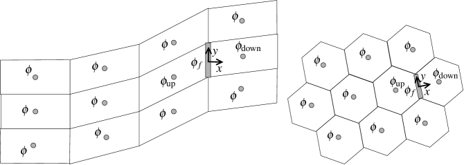
Figure 1: Stencils of upwind-biased cells for interpolating onto face $f$ using a 2d cubic polynomial for two different mesh structures.

In order to ensure that the fit is accurate in the cells either side of face $f$ and to ensure that the values in these adjacent cells have the strongest control over $\phi_{f}$, rows associated with these values in the least squares fit matrix are weighted a factor of 1000 relative to the other rows (following Lashley, 2002). This does not affect the order of accuracy. Mathematically, an arbitrarily large value of the weight can be used to ensure that the fit goes exactly through the upwind and downwind cell. However if a value too large is used, the singular value problem becomes ill conditioned. We do not use any of the other stabilisation procedures as described by SWMD1x. The value $\phi_{f}$ is then calculated as a higher-order correction to first-order upwind:

$$\phi_{f}=\phi_{\text{up}}+\sum_{c}w_{c}\phi_{c}$$ (19)

where $w_{c}$ are the weights for each cell of the stencil calculated from the least squares fit, with $w_{\text{up}}$ reduced by 1 to make the fit a correction on upwind.

2.3.1 Implicit Solution, Matrix Solvers and Tolerances

The trapezoidal implicit or Crank-Nicholson time-stepping leads to a matrix equation which needs to be solved to find all the $\phi$s at the next time-step. In order to ensure that the matrix is diagonally dominant for arbitrary time-steps, the cubic interpolation applied is a deferred correction on first-order upwind so that only the coefficient corresponding to the upwind cells are included in the matrix. This means that more than one implicit solves are needed per time-step so that the higher-order terms are solved to be second-order accurate in time. If the Courant number is less than or close to one, we use two implicit solves per time-step. Consequently, assuming that the velocity field and mesh are constant in time, the time-stepping scheme is defined as:

$$\frac{\phi^{\prime}-\phi^{n}}{\Delta t} = -\frac{1}{2V}\sum_{f\in c}\left(\phi_{\text{up}}^{n}+\phi_{\text{up}}^{\prime}+2\sum_{c}w_{c}\phi_{c}^{n}\right)\mathbf{u}_{f}\cdot\mathbf{S}_{f}$$ (20)

$$\frac{\phi^{n+1}-\phi^{n}}{\Delta t} = -\frac{1}{2V}\sum_{f\in c}\left(\phi_{\text{up}}^{n}+\phi_{\text{up}}^{n+1}+\sum_{c}w_{c}\phi_{c}^{n}+\sum_{c}w_{c}\phi_{c}^{\prime}\right)\mathbf{u}_{f}\cdot\mathbf{S}_{f}.$$ (21)

For larger Courant numbers we use four implicit solves per time-step although sensitivity to this choice has not been investigated.

If this implicit scheme is applied on a logically rectangular, two-dimensional mesh with horizontal and vertical Courant numbers $c_{x}$ and $c_{z}$, then the diagonal coefficients of the matrix would be $1+c_{x}/2+c_{z}/2$ and, assuming two upwind directions, there would be exactly two off-diagonal elements, $-c_{x}/2$ and $-c_{z}/2$. Consequently the matrix is very sparse, asymmetric and diagonally dominant for all time-steps. It is solved using the OpenFOAM bi-conjugate gradient solver using DILU pre-conditioning to a tolerance of $10^{-8}$ every iteration. Sensitivity to the solver or solver tolerance have not been investigated. Information about the number of solver iterations for different test cases in given in section 3.4.

3 Results of Test Cases in Planar Geometry

In order to make test cases as simple as possible without the need for incorporating spherical geometry, multi-panel meshes or non-rectangular cells, our computational domain consists of a periodic two-dimensional plane with deformations in the co-ordinate system (or mesh) mimicking the kind of distortions which are produced by a cubed-sphere mesh. We also use a two-dimensional vertical slice test case over orography using terrain following co-ordinates (or terrain following meshes).

A range of test cases are undertaken on uniform and distorted meshes using the dimensionally split scheme and the multi-dimensional scheme in order to evaluate the influences of mesh distortions, the validity of using a dimensionally split scheme on a distorted mesh and the schemes’ accuracy and stability for long time-steps.

3.1 Solid Body Rotation

The solid body rotation test case of Leonard et al. (1996a) is used to compare the accuracy of the dimensionally split and multi-dimensional schemes on orthogonal and non-orthogonal meshes. We define this test case on a domain that is $10^{4}\times 10^{4}\text{ m}^{2}$. The velocity is defined by numerically differentiating the streamfunction which can be defined at mesh vertices, $\mathbf{x}$, by:

$$\psi(\mathbf{x},t)=A|\mathbf{x}-\mathbf{x}_{c}|^{2}$$ (22)

where $\mathbf{x}_{c}$ is the centre of the domain, and $A=5\pi/3000\text{ s}^{-1}$ so that the angular velocity is $2A$. The initial tracer takes a Gaussian distribution in order to ensure that all advection schemes achieve their theoretical order of accuracy:

$$\phi(\mathbf{x})=\exp\left(-\frac{1}{2}\frac{|\mathbf{x}-\mathbf{x}_{\phi}|^{2}}{r_{\phi}^{2}}\right)$$ (23)

where $\mathbf{x}_{\phi}=\mathbf{x}_{c}+r_{c\phi}\mathbf{j}$ is the initial centre of the tracer distribution, $r_{c\phi}=2500\text{ m}$, $r_{\phi}=500\text{ m}$ and $\mathbf{j}$ is the unit vector in the $y$ direction. The analytic solution has the same tracer distribution but with the centre of the tracer at:

$$\mathbf{x}_{\phi}=\mathbf{x}_{c}+r_{c\phi}\left(\begin{array}[]{c}\cos(\pi/2+2At)\\ \sin(\pi/2+2At)\end{array}\right)$$ (24)

and the Gaussian rotates anti-clockwise exactly one revolution in $600\text{ s}$.

The solid body rotation test case is performed on a uniform, orthogonal mesh and on a non-orthogonal mesh on a plane with non-orthogonality similar to that of a cubed-sphere mesh. For the dimensionally split scheme, non-orthogonality is achieved using the co-ordinate transform:

$$\begin{array}[]{ccc}X=x&&Y=\begin{cases}y_{m}\left(1+\frac{y-f}{2y_{m}-f}\right)&\text{ for }y\geq f\\ y_{m}\left(1+\frac{y-f}{f}\right)&\text{ for }y<f\end{cases}\end{array}$$ (25)

where $y_{m}=5000\text{ m}$ and $f$ is the equation for a $y$ position of uniform $Y$ half way up the domain. In order to create angles of $120^{o}$ in the mesh, similar to a cubed-sphere, $f$ is given by:

$$f=\begin{cases}y_{m}\left(1+\frac{1}{2\sqrt{3}}\right)-\frac{x}{\sqrt{3}}&\text{ for }x\leq x_{m}\\ y_{m}\left(1-\frac{1}{2\sqrt{3}}\right)+\frac{x-x_{m}}{\sqrt{3}}&\text{ for }x>x_{m}\end{cases}.$$ (26)

where $x_{m}=5000$ m. For a $50\times 50$ mesh this gives the $x$ and $y$ co-ordinate locations as shown in figure 2. The multi-dimensional scheme model uses Cartesian co-ordinates and a distorted mesh rather than a non-orthogonal co-ordinate system on a Cartesian mesh. However this does not affect the numerical results assuming that the co-ordinate transforms are implemented in a consistent way to the distorted mesh in Cartesian co-ordinates.

For the dimensionally split scheme, bi-periodic boundary conditions are applied. For the multi-dimensional scheme, it was more straightforward to impose fixed value boundary conditions of $\phi=0$ where the velocity is into the domain and zero normal gradient where the velocity is out of the domain. However $\phi$ remains almost zero near the boundaries so these boundary conditions do not affect the accuracy.

Figure 2: Two non-orthogonal mesh on a plane with $50\times 50$ mesh points and angles up to $120^{\text{o}}$ designed to have similar angles to a cubed-sphere mesh.

Results of this test case on the orthogonal and non-orthogonal meshes of $100\times 100$ cells with $\Delta t=1\text{ s}$ are shown in figure 3 for both advection schemes (which gives a maximum Courant number close to one). The contours show the tracer value every 100 seconds and the colours show the errors summed every 100 seconds. The dimensionally split scheme outperforms the multi-dimensional scheme on both meshes due to the higher-order accuracy of the split scheme. The dimensionally split scheme introduces a small error at 300 seconds where the tracer goes through the change in direction of the mesh which would be ameliorated if we were using monotonicity constraints. The second-order, multi-dimensional scheme shows phase lag but errors are almost entirely insensitive the mesh distortions.

Figure 3: Results of the solid body rotation test case on orthogonal and non-orthogonal meshes every 100 seconds for meshes of $100\times 100$ cells and $\Delta t=1\text{ s}$ giving a maximum Courant number of around 1. The contours show the tracer value from 0.1 every 0.1 to 0.9 and the colours show the errors. The dashed contour shows the initial conditions. The min and max text in each plot gives the minimum and maximum errors.

The multi-dimensional and dimensionally split schemes take very different approaches to handling large Courant numbers. The multi-dimensional scheme uses implicit time-stepping whereas the dimensionally split scheme uses a flux-form semi-Lagrangian approach, integrating over a line of cells in order to calculate the flux across a face. Implicit schemes are known to suffer from phase errors (eg DB12; LWW14) for long time-steps whereas the accuracy of semi-Lagrangian is less sensitive to time-step (PS84). Therefore we present results of both schemes on orthogonal and non-orthogonal meshes for time-steps 10 times those used in figure 3 ($\Delta t=10\text{ s}$) giving maximum Courant numbers of around 10 using $100\times 100$ cells in figure 4. The error of the multi-dimensional scheme is again much larger than the dimensionally split scheme on both meshes. The dimensionally split scheme is accurate at large Courant numbers despite the first-order calculation of departure points. However, the dimensionally split scheme introduces oscillations on the non-orthogonal mesh, particularly where the mesh changes direction whereas for the multi-dimensional scheme, errors are not strongly affected by the non-orthogonality. Figure 4 clearly shows phase errors of the implicit time-stepping but, despite the large Courant number, the well resolved part of the profile is propagating at close to the correct speed. Dispersion analysis (LWW14) shows that high frequency oscillations (which are poorly resolved in time and space) will be slowed dramatically but fast moving features which are well resolved in space will propagate at a much more realistic speed, supporting the results shown in figure 4.

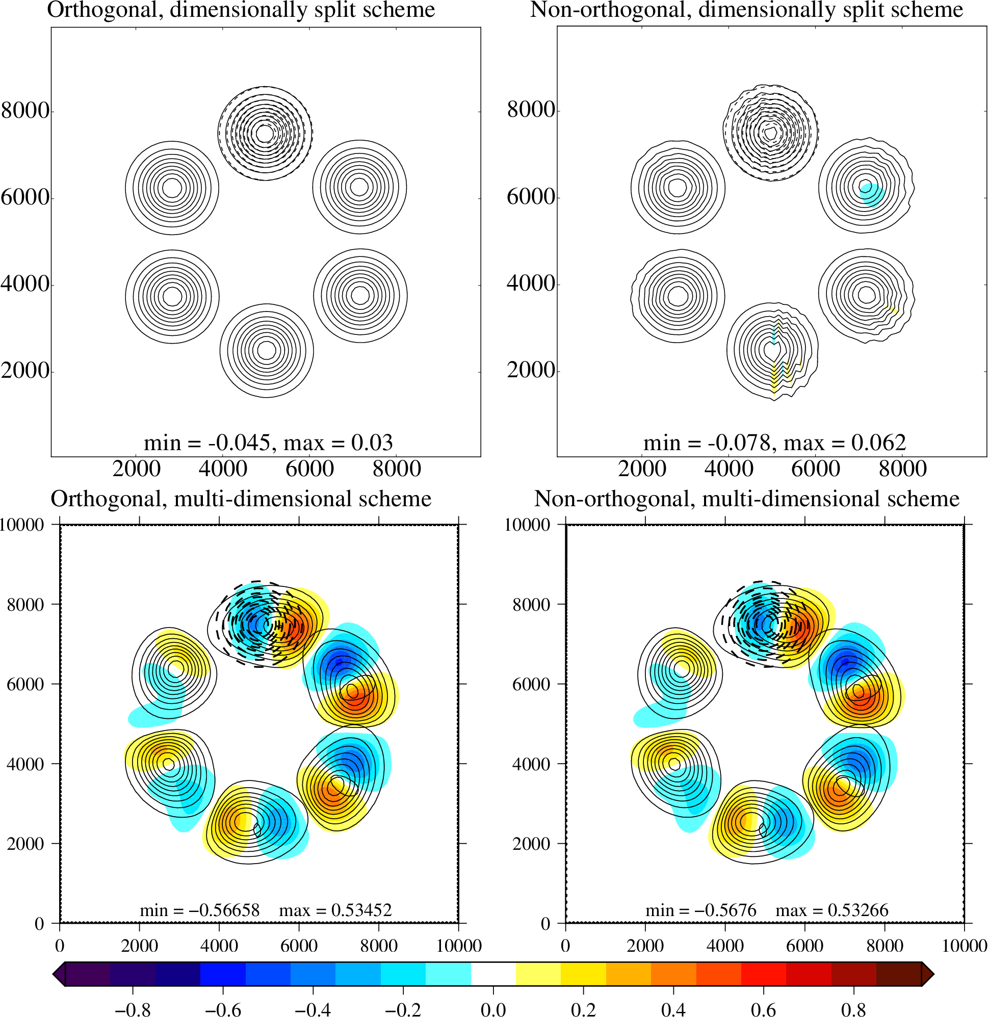
Figure 4: Results of the solid body rotation test case on orthogonal and non-orthogonalmeshes every 100 seconds for meshes of $100\times 100$ cells and $\Delta t=10\text{ s}$ giving a maximum Courant number of around 10. The contours show the tracer value from 0.1 every 0.1 to 0.9 and the colours show the errors. The dashed contour shows the initial conditions. The min and max text in each plot gives the minimum and maximum errors.

In order to compare convergence with resolution of the different numerical methods, we use the $\ell_{2}$ and $\ell_{\infty}$ error norms defined in the usual way:

$$\ell_{2} = \sqrt{\int_{V}\left(\phi-\phi_{T}\right)^{2}dV\bigg{/}\int_{V}\phi_{T}^{2}\ dV}$$ (27)

$$\ell_{\infty} = \max|\phi-\phi_{T}|\big{/}\max|\phi_{T}|$$ (28)

where $\phi_{T}$ is the analytic solution and the integrations and maxima are over the whole domain, with volume $V$. Figure 5 shows convergence with resolution of the $\ell_{2}$ and $\ell_{\infty}$ error measures for meshes of $50\times 50$, $100\times 100$, $200\times 200$ and $400\times 400$ cells with time-steps scaled in order to maintain a maximum Courant number of 1 ($\Delta t=2,\ 1,\ 0.5,\ 0.25\text{ s}$) or scaled to achieve a maximum Courant number of 10 ($\Delta t=20,\ 10,\ 5,\ 2.5\text{ s}$). The error norms are calculated at $t=500\ \text{seconds}$, when the tracer has made $5/6$ of one revolution in order to avoid error cancellation. On both orthogonal and non-orthogonal meshes, the multi-dimensional scheme has second order convergence once errors are low enough to avoid error saturation (stable errors are bounded at around one). With a large Courant number, both schemes are less accurate. For the multi-dimensional scheme, this is due to phase errors of the implicit time-stepping whereas for the multi-dimensional scheme the first-order errors in calculating the departure point and trajectory will be emerging and there could also be significant errors from the second-order COSMIC splitting. On the orthogonal mesh, the dimensionally split scheme has third order convergence for the Courant number close to one and second order for the larger Courant number (consistent with the results of Colella and Woodward, 1984a; Leonard et al., 1996a). On the non-orthogonal mesh, the dimensionally split scheme has second order converges for both Courant numbers.

Figure 5: Convergence with spatial resolution of the $\ell_{2}$ and $\ell_{\infty}$ errors for the solid body rotation test case at $t=500\ \text{seconds}$ ($5/6$ of one revolution) on orthogonal and non-orthogonal meshes using multi-dimensional and dimensionally split schemes.

The different time-stepping schemes of the two models also affect accuracy. The $\ell_{2}$ and $\ell_{\infty}$ error measures as a function of time-step for meshes of $100\times 100$ cells are shown in figure 6. The dimensionally split scheme, which uses flux-form semi-Lagrangian time-stepping, has errors reducing as time-step increases, up to a Courant number of 2 ($\Delta t=2\ \text{s}$) whereas the multi-dimensional scheme, which uses the method of lines to treat space and time separately, always has error reducing as time-steps reduces. The flux-form semi-Lagrangian technique discretises space and time together and the error is not very sensitive to time-step. However, the shorter the time-step, the more time-steps need to be taken so errors can actually accumulate more by taking more time-steps. (This is consistent with the order of accuracy of semi-Lagrangian being $\Delta x^{p}/\Delta t$ for interpolation using polynomials of degree $p$, as described by Dur10.)

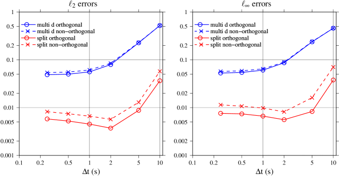
Figure 6: Convergence with temporal resolution of the $\ell_{2}$ and $\ell_{\infty}$errors for the solid body rotation test case at $t=500\ \text{seconds}$ ($5/6$ of one revolution) using orthogonal and non-orthogonal meshes of $100\times 100$ cells using multi-dimensional and dimensionally split schemes. Maximum Courant numbers range from $c=0.25$ (for $\Delta t=0.25\ \text{s})$ to $c=10$ (for $\Delta t=10\ \text{s})$.

In summary, the dimensionally split scheme has excellent behaviour at large and small Courant numbers on the orthogonal meshes with up to third order convergence for small Courant numbers and the errors increase and order of convergence decreases on non-orthogonal meshes. In contrast, the multi-dimensional scheme is insensitive to the orthogonality, converges with second-order and suffers from phase errors at large Courant numbers.

3.2 Horizontal Advection over Orography

Non-orthogonal meshes (or co-ordinate systems) are usually necessary for representing orography which could be a challenge for dimensionally split schemes. Horizontal-vertical split schemes are commonly used in this context (eg. DEE+12; WGZ+13). We present results of the SLF+02 horizontal advection over orography test case for a range of resolutions and Courant numbers for the dimensionally split and multi-dimensional schemes.

All simulations use basic terrain following co-ordinates (BTF, Gal-Chen and Somerville, 1975) in order to present a challenging test case that maximises the non-orthogonality. The transformation is given by:

$$\begin{array}[]{ccc}X=x&&Z=H\frac{z-h(x)}{H-h(x)}\end{array}$$ (29)

where $H$ is the domain height and $h$ is the terrain height. The test case uses a domain of width 300 km, height, $H=25\text{ km}$ and a mountain range defined by

$$h=\begin{cases}h_{0}\cos^{2}\frac{\pi x}{\lambda}\cos^{2}\frac{\pi x}{2a}&\text{ for }|x|\leq a\\ 0&\text{ otherwise}\end{cases}$$ (30)

with the maximum mountain height, $h_{0}=3\text{ km}$, half-width $a=25\text{ km}$ and wavelength $\lambda=8\text{ km}$. These values give a maximum terrain gradient of close to $45^{o}$. The wind is given by a streamfunction which is defined at vertices so that the wind field is discretely divergence free. The streamfunction at vertices is calculated analytically from the wind profile:

$$u(z)=u_{0}\begin{cases}1&\text{ for }z_{2}\leq z\\ \sin^{2}\left(\frac{\pi}{2}\frac{z-z_{1}}{z_{2}-z_{1}}\right)&\text{ for }z_{1}<z\leq z_{2}\\ 0&\text{ for }z<z_{1}\end{cases}$$ (31)

with $u_{0}=10\text{ ms}^{-1}$, $z_{1}=4\text{ km}$ and $z_{2}=5\text{ km}$. The initial tracer position is given by:

$$\phi=\begin{cases}\cos^{2}\frac{\pi r}{2}&\text{ for }r\leq 1\\ 0&\text{ otherwise}\end{cases}\text{ with }r=\sqrt{\left(\frac{x-x_{0}}{A_{x}}\right)^{2}+\left(\frac{z-z_{0}}{A_{z}}\right)^{2}}$$ (32)

with initial tracer centre, $(x_{0},z_{0})=(-50\text{ km},\ 9\text{ km})$ and halfwidths $A_{x}=25\text{ km}$, $A_{z}=9\text{ km}$. At time $t=5000\text{ s}$ the tracer is above the mountain and the simulation finishes at $t=10,000\text{ s}$ by which time the analytic solution is centred at $(50\text{km },8\text{km})$.

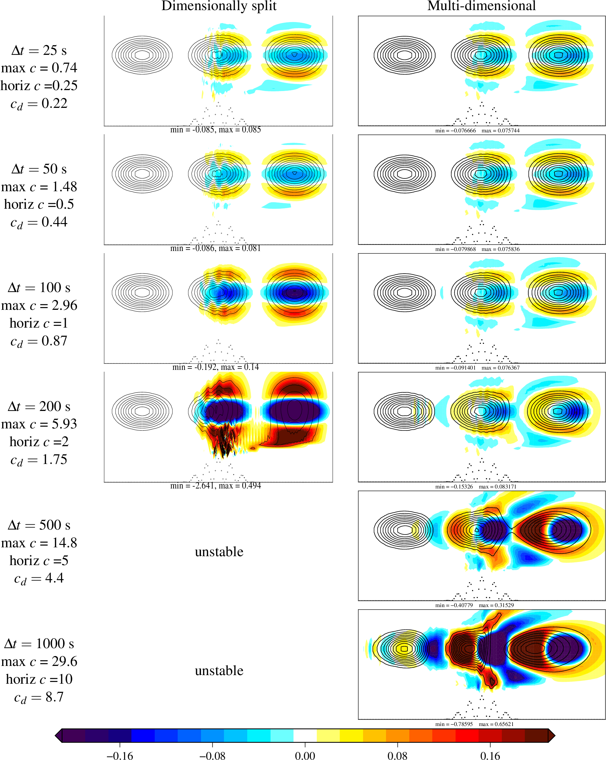
Figure 7: Tracer contours after 0, 5000 and 10000s for the horizontal advection over orography and errors in colour. Different plots use different time-steps. Spatial resolution is $\Delta x=1\$km, $\Delta z=500\$m. Maximum Courant numbers, horizontal Courant number, $c$, and maximum deformational Courant number, $c_{d}$ are also given.

The tracer advection over orography is shown in figure 7 for the split and multi-dimensional schemes at a resolution of $\Delta x=1\text{ km}$, $\Delta z=500\text{ m}$ and for a range of Courant numbers. The horizontal Courant number is defined as $u_{0}\Delta t/\Delta x$ and ranges from 0.25 to 10. The maximum Courant number is the maximum of the multi-dimensional Courant number which is defined for cell with faces $f$ as:

$$c=\frac{1}{2V}\sum_{f}|\mathbf{u}_{f}\cdot\mathbf{S}_{f}|\Delta t$$ (33)

(see section 2.3 for definitions of variables) and ranges from 0.74 to 29.6. The time-step restriction for the split scheme is based on the deformational Courant number, $c_{d}\leq 1$, (eqn 10). The maximum deformational Courant number is also given in figure 7. The contours in figure 7 show the tracer values at 0, $5000\text{ s}$ and $10,000\text{ s}$ after initialisation and the colours show the errors from the analytic solution. For horizontal Courant numbers less than one (maximum Courant number up to 3), both schemes give accurate results with the dimensionally split scheme tending to give oscillations and the multi-dimensional scheme producing more diffusion. For larger Courant numbers, when the deformational Courant number is greater than one, the split scheme is unstable while the multi-dimensional scheme produces large phase errors due to the errors associated with implicit time-stepping. The term responsible for the large deformational Courant number is $\partial u/\partial z$ where the velocity shears from $u_{0}=10$m/s at $z=z_{2}$ to zero at $z=z_{1}$.

We examine the convergence with resolution in figure 8 which shows the $\ell_{2}$ and $\ell_{\infty}$ error norms as a function of $\Delta x$. These simulations all use a maximum Courant number less than one, a horizontal Courant number of 0.25, a maximum deformational Courant number of about 0.2 and fixed ratios of $\Delta x$, $\Delta z$ and $\Delta t$. Both schemes give similar accuracy with the dimensionally split scheme having faster convergence with resolution.

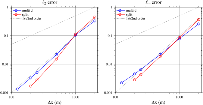
Figure 8: Convergence of the $\ell_{2}$ and $\ell_{\infty}$ error metricsfor horizontal advection over a 3000m and a 6000m mountains after 10,000s for the dimensionally split (PPM) scheme and multi-dimensional MOL scheme, all using a horizontal Courant number of 0.25. Lines also show theoretical first- and second-order convergence are also shown.

In summary, the dimensionally split scheme has good accuracy over orography for modest Courant numbers but larger errors for larger Courant numbers and is unstable when the deformational Courant number is greater than one whereas the multi-dimensional scheme with implicit time-stepping is stable for all Courant numbers. The multi-dimensional scheme second-order convergent and the dimensionally split scheme converges faster.

3.3 Deformational Flow

In deformational flow, there is no analytical solution and therefore we follow the approach of NL10; Lauritzen et al. (2012b) and define an evolving velocity field that reverses direction half way through the simulation, taking the tracer back to the initial conditions. Error norms can then be calculated by comparing the final and initial tracer fields. The deformational velocity field is added to a fixed solid body rotation that does not reverse so as to avoid error cancellation between the forwards and backwards periods (solid body here meaning horizontal wind on a periodic domain).

We define a Cartesian version of the deformational, non-divergent test case of Lauritzen et al. (2012b) with a domain between $-\pi$ and $\pi$ in the $x$ direction ($L_{x}=2\pi$) and between $-\frac{\pi}{2}$ and $\frac{\pi}{2}$ in the $y$ direction ($L_{y}=\pi$) with periodic boundary conditions in the $x$ direction and zero gradient, zero flow boundary conditions in the $y$ direction. The stream function adapted to Cartesian co-ordinate is:

$$\psi\left(x,y,t\right) = \frac{\hat{\psi}}{T}\left(\frac{L_{x}}{2\pi}\right)^{2}\sin^{2}\left(2\pi\left(\frac{x}{L_{x}}-\frac{t}{T}\right)\right)\cos^{2}\left(\pi\frac{y}{L_{y}}\right)\cos\left(\pi\frac{t}{T}\right)-L_{x}\frac{y}{T}$$ (34)

where $\hat{\psi}=10$ and $T=5$ is the time for one complete revolution of the periodic domain for the solid body rotation part of the flow. In order to test the order of convergence of the advection schemes, we use the infinitely smooth Gaussian distribution for the initial tracer concentration:

$$\phi=0.95\exp-\frac{|\mathbf{x}-\mathbf{x}_{0}|^{2}}{A}+0.95\exp-\frac{|\mathbf{x}-\mathbf{x}_{1}|^{2}}{A}$$ (35)

where $\mathbf{x}^{T}=(x,y)$, $\mathbf{x}_{0}^{T}=(\frac{5}{12}L_{x},0)$, $\mathbf{x}_{1}^{T}=(\frac{7}{12}L_{x},0)$ and $A=\frac{1}{5}$.

A mesh with distortion similar to a cubed-sphere is defined by the co-ordinate transform:

$$\begin{array}[]{ccc}X=x&&Y=\begin{cases}L_{y}\frac{y-f}{L_{y}-2f}&\text{ for }y\geq f\\ L_{y}\frac{y-f}{L_{y}+2f}&\text{ for }y<f\end{cases}\end{array}$$ (36)

where $f$ is:

$$f=\begin{cases}\frac{1}{\sqrt{3}}\left(\frac{\pi}{4}-|x|\right)&\text{ for }|x|\leq\frac{\pi}{2}\\ \frac{1}{\sqrt{3}}\left(|x|-\frac{3\pi}{4}\right)&\text{ for }|x|>\frac{\pi}{2}\end{cases}.$$

The initial conditions and a $120\times 60$ mesh with distortion defined by this co-ordinate transform is shown in figure 9.

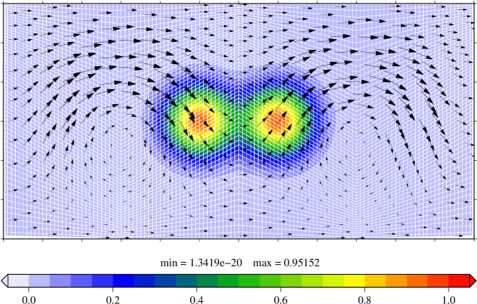
Figure 9: The non-orthognal mesh/co-ordinate system for the deformational flow with $120\times 60$ cells and the initial tracer conditions.

The tracer concentrations after 1, 2, 3, 4 and 5 time units are shown in figure 10 using the dimensionally split and multi-dimensional schemes on a non-orthogonal mesh of $480\times 240$ cells, a time-step of 0.0025 units (ie 2000 time-steps to reach 5 time units) which gives a maximum Courant number of 1.03. The tracer is stretched out, wound up, advected around and then wound back into its original position with some numerical errors. Both advection schemes preserve fine filaments but suffer from some dispersion errors which generate small oscillations around zero behind sharp gradients in the direction of the flow since neither scheme is monotonic or positive preserving. The dimensionally split scheme returns the tracer to a more accurate final solution.

Figure 10: Results of the deformational flow test case after 1, 2, 3, 4 and 5 time units on the non-orthogonal meshes of 480$\times$240 cells using the multi-dimensional and split schemes.

Resolution	$60\times 30$	$120\times 60$	$240\times 120$	$480\times 240$	$960\times 480$	$1920\times 960$
$\Delta t$ $\downarrow$	Maximum Courant numbers (deformational) $\downarrow$
0.2	10.3 (0.639)
0.1		10.3 (0.312)
0.05		5.17 (0.154)	10.3 (0.154)
0.025				10.3 (0.077)
0.02		2.06 (0.061)
0.0125	1.03				10.3
0.01		1.03 (0.030)
0.00625						10.3
0.005		0.517 (0.015)	1.03 (0.015)
0.0025		0.254 (0.008)		1.03 (0.008)
0.00125					1.03 (0.004)
0.000625						1.03

Table 1: Resolutions, time-steps and Courant numbers for the non-orthogonal meshes for the deformational flow test case. Maximum Courant numbers are shown inside the table for simulations which are presented in graphs. The maximum Courant numbers on the orthogonal meshes are 70% of those on the non-orthogonal meshes. The maximum deformational Courant numbers are in brackets for some cases

Sensitivity to orthogonality, resolution and time-step are explored using a range of simulations with maximum Courant numbers shown in table 1. The Courant numbers on the uniform, orthogonal meshes (with no mesh distortions) are 70% of those on the non-orthogonal mesh since the non-orthogonal mesh has clustering of mesh points. The deformational Courant number is less than one for all simulations. The convergence with resolution of the $\ell_{2}$ and $\ell_{\infty}$ error norms at the final time are shown in figure 11 for both advection schemes using a maximum Courant number close to one and for a maximum Courant number close to ten. We will first consider the behaviour of the schemes at modest Courant number (maximum close to one). All of the schemes give first-order convergence with resolution at coarse resolutions due to error saturation (if the scheme is stable, errors are bounded above by about one). At higher resolution, the split scheme converges with nearly third-order for both meshes whereas the multi-dimensional scheme approaches second-order. For large Courant numbers (maximum close to 10), the split scheme converges with first-order for both mesh types due to the crude estimation of the departure point (section 2.1) whereas the multi-dimensional scheme is much less accurate but approaches second-order at high resolution. The dimensionally split scheme is sensitive to mesh distortions only for large Courant numbers.

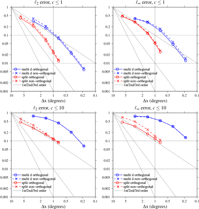
Figure 11: Convergence with resolution of the $\ell_{2}$ and $\ell_{\infty}$ errors for the deformational flow on orthogonal and non-orthogonal meshes using multi-dimensional and dimensionally split schemes.

We inspect sensitivity to time-step of both schemes on orthogonal and non-orthogonal meshes of $120\times 60$ cells in figure 12 using the time-steps shown in table 1 giving maximum Courant numbers ranging from 0.25 to 10 (deformational Courant numbers always less than 0.32). This demonstrates potentially useful properties of the flux-form semi-Lagrangian time-stepping used by the split scheme. Ignoring errors in calculating the departure point, semi-Lagrangian schemes have errors proportional to $\Delta t^{-1}$ (Dur10) which explains the reduction in error as time-step increases for the split scheme. Once the maximum Courant number reaches 1 or 2 ($\Delta t=0.01$ or 0.02), errors of the split scheme do grow with the time-step, due to the deformational nature of the flow and errors in calculating the departure points. In contrast, using the multi-dimensional scheme which uses method of lines time-stepping, errors always increase as the time-step is increased. Comparisons between schemes in figures 10 and 11 used maximum Courant numbers of 1 and 10 which showed that the split scheme on the orthogonal mesh gave better accuracy than the multi-dimensional scheme. However, figure 12 shows that this advantage disappears at lower Courant numbers since the multi-dimensional scheme (method of lines) gets more accurate with lower Courant numbers whereas the split scheme (semi-Lagrangian) gets less accurate since more time-steps have to be taken. Both schemes are stable for all time-steps considered.

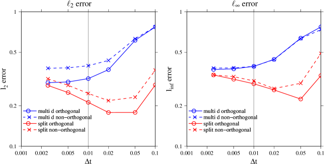
Figure 12: Variation of $\ell_{2}$ and $\ell_{\infty}$ errors with time-step for the deformational flow on orthogonal and non-orthogonal meshes of $120\times 60$ cells using multi-dimensional and dimensionally split schemes. Different time-steps give maximum Courant numbers of 0.25, 0.5, 1, 2, 5 and 10.

In summary, the dimensionally split scheme has good accuracy for deformational flow independent of mesh orthogonality. The multi-dimensional scheme is competitive at small Courant numbers but the semi-Lagrangian nature of the split scheme means that errors are very low for Courant numbers close to one.

3.4 Computational Cost

We cannot compare CPU time, wall clock time or parallel efficiency of the two advection schemes because the multi-dimensional scheme is written in C++ using OpenFOAM and the split scheme is written in Python, both codes have been run on different hardware and the split advection scheme code has not been parallelised. Instead we consider the number of multiply operations performed per cell per time-step for calculating the fluxes of each tracer. We appreciate that this is not a good predictor of efficiency as it does not consider memory read and write requirements or cache coherency. However all data that is multiplied has to be fetched from memory and so, assuming that all data can be arranged optimally in memory to enable fewest cache misses, the number of multiplies should be related to the wall clock time. Neither advection scheme does significantly more work per memory fetch than the other.

For both schemes we consider the number of multiplies needed to calculate the flux of $\phi$ at each face. That is equation 7 for the dimensionally scheme and equation (19) for the multi-dimensional scheme. We do not consider the computational cost of updating the cell averages from the fluxes using Gauss’s theorem (eqns (3) and (17)) as these are the same for each scheme. For the multi-dimensional scheme, we do include an estimate of the amount of work done by the linear equation solver but we do not consider the scalability of this solver.

3.4.1 Dimensionally Split Scheme

The computational cost of PPM with COSMIC splitting is not strongly time-step dependent due to the swept area approach of flux-form semi-Lagrangian. One-dimensional PPM uses 4 cells for interpolation to find face values used by the reconstruction. Assuming as much as possible is pre-computed, this interpolation uses 3 multiplies on a non-uniform mesh. The reconstruction then uses 6 multiplies to calculate the flux on each face. Only one additional memory access and one additional multiply are needed per cell for Courant numbers greater than one (eqn 8) making 10 multiplies per cell for applying PPM in one direction for a Cournat number greater than one. The COSMIC splitting in two dimensions involves four applications of the one-dimensional PPM. This makes 40 multiplies per cell in total for applying PPM with COSMIC splitting in two dimensions. In three dimensions, COSMIC splitting requires 12 applications of PPM (Leonard et al., 1996a) leading to 120 multiplies.

3.4.2 Multi-dimensional Scheme

The number of multiplies involved in the multi-dimensional scheme includes the number of multiplies to update the higher order advection and the number of multiplications for each iteration of the linear equation solver. We will also consider the cost of an explicit version of the multi-dimensional scheme using an RK2 time-stepping scheme (eg as used by SW16) which is stable and accurate up to a Courant number of one for this spatial discretistion and gives very similar results to the implicit scheme (not shown).

The explicit version of the dimensionally split scheme uses RK2 or Heun time-stepping, in which $\phi_{\text{up}}^{\prime}$ on the RHS of eqn (20) is replaced by $\phi_{\text{up}}^{n}$ and $\phi_{\text{up}}^{n+1}$ on the RHS of eqn (21) is replaced by $\phi_{\text{up}}^{\prime}$. On a logically rectangular two-dimensional mesh there are 12 cells in each stencil for each face (fig 1). Each cell has four faces and the interpolation onto each face is used to calculate the flux between two cells. This leads to 24 multiplies per cell for each RK2 stage and hence 48 multiplies per cell per time-step. When using implicit time-stepping, there will be 24 multiplies per cell for every evaluation of the right hand side of the matrix for the higher-order correction on first-order upwind.

We have not explored the sensitivity of the accuracy and stability to the stencil size and shape in three dimensions. The three dimensional equivalent of the stencil of quadrilaterals in figure 1 is likely to contain 36 (rather than 12) cells although it may be possible to omit some corner cells and use a stencil of 20 cells. For a stencil of 36 cells, the number of multiplies per cell per time-step would be $36\times 3\times 2=216$.

The implicit version of the multi-dimensional scheme (section 2.3.1) requires the solution of an asymmetric, diagonally dominant matrix with three non-zero elements per row for a logically rectangular two-dimensional mesh. The pre-conditioner is implemented in file DILUPreconditioner.C in OpenFOAM 3.0.1 and the solver in file PBiCG.C. From these files, we estimate that, for a mesh of quadrilaterals, the solver will use 24 multiplies (or divides) per cell, per solver iteration, including pre-conditioning. The average number of iterations of the preconditioned bi-CG solver per time-step for each of the simulations is shown in table 2 (including the number of solver iterations in each outer iteration). These simulations use two outer iterations per time-step when the maximum Courant number is $\leq 1.1$ (as in equations (20) and (21)) but, for stability, use four outer iterations per time-step for the larger Courant numbers. This partly explains the greater number of iterations for larger Courant numbers. A solver tolerance of $10^{-8}$ is used for each of the outer solves. Table 2 shows that the total number of iterations per time-step reduces slightly as resolution increases. The total number of iterations for a complete simulation is reduced by using larger Courant numbers because the number of iterations per time-step increases less than linearly with increasing Courant numbers. In fact, simulations with larger Courant numbers are considerably cheaper because there are fewer evaluations of the right hand side of the matrix equation.

Resolution $\rightarrow$	$120\times 60$	$240\times 120$	$480\times 240$	$960\times 480$	$1920\times 960$
Max $c$ $\downarrow$	Iterations per time-step orthogonal/non-orthogonal $\downarrow$
10	33.4/39.5	31.3/38.0	26.0/32.8	19.3/25.0	13.5/18.6
5	22.4/25.7
2	13.1/14.6
1	6.0/6.5	5.4/5.8	4.9/5.3	4.6/4.9	3.9/4.2
0.5	4.9/5.0
0.25	3.9/3.9

Table 2: Number of solver iterations per time-step of the multi-dimensional scheme for all the simulations on orthogonal/non-orthogonal meshes.

Combining the number of solver iterations, the number of multiply operations per solve and the number of multiply operations in calculating the explicit higher order part of the advection scheme, the total number of multiply operations per cell per time-step for the multi-dimensional scheme is shown in table 3 for the non-orthogonal mesh of $120\times 60$ cells. Table 3 also shows the number of multiplies for using the explicit, RK2 version of the multi-dimensional scheme and the dimensionally split scheme.

Max $c$	Implicit	Explicit	Dimensionally
	Multi-dimensional		Split
10	$39.5\times 24+48\times 2=1,044$	-	40
5	$25.7\times 24+48\times 2=712.8$	-	40
2	$14.6\times 24+48\times 2=446.4$	-	40
1	$6.5\times 24+48=204$	48	40
0.5	$5.0\times 24+48=168$	48	40
0.25	$3.9\times 24+48=$141.6	48	40

Table 3: Total number of multiply operations per cell per time-step for different Courant numbers for the multi-dimensional scheme, an explicit version of the multi-dimensional scheme (using RK2 or Heun time-stepping) and the dimensionally split scheme on two-dimensional, logically rectangular meshes. The multi-dimensional scheme using RK2 time-stepping is stable for Courant numbers $\leq 1$ and gives very similar solutions to the implicit version.

Table 3 shows that the implicit scheme always uses more multiply operations but particularly uses more multiplies for large Courant numbers. The explicit version of the multi-dimensional scheme always uses 48 multiply operations but is not stable for all time-steps whereas the dimensionally split scheme (using flux-form semi-Lagrangian time-stepping) is stable for all Courant numbers (at this spatial resolution) and always uses the fewest number of multiply operations per cell per time-step.

There is considerable flexibility in the solver configuration: the number of outer iterations per time-step determines how frequently the high-order correction on the right hand side of the matrix equation is updated, and the solver tolerance per outer iteration could be modified by using a weaker tolerance on all but the final matrix solve per time-step. These options have not been explored. It may also be beneficial to create more non-zero matrix entries rather than having the higher-order correction entirely a deferred correction on first-order upwind, but such a change would need to ensure that the matrix remains diagonally dominant.

4 Summary and Conclusions

We examine the errors associated with using a dimensionally split advection scheme and a multi-dimensional advection scheme on distorted meshes. The dimensionally split scheme is very accurate on orthogonal meshes and only loses a little accuracy on highly distorted meshes, despite a first-order departure point calculation. The multi-dimensional scheme with implicit time-stepping is less accurate on orthogonal meshes than the dimensionally split scheme but the accuracy is not sensitive to mesh distortions and the stability is less sensitive to Courant number.

The dimensionally split scheme is the piecewise polynomial method (PPM, Colella and Woodward, 1984a) with COSMIC splitting (Leonard et al., 1996a) that extends it to two spatial dimensions. PPM is converges with third-order in one dimension and COSMIC splitting enables second-order convergence in two orthogonal directions. PPM is a flux-form semi-Lagrangian scheme and so can handle large Courant numbers accurately without significant additional computational cost, with a time-step restriction based on the deformational Courant number. The second-order accurate multi-dimensional scheme is split in space and time (method of lines) and uses a cubic polynomial fit over a stencil of cells for spatial discretisation and trapezoidal implicit in time to retain stability for large Courant numbers. We use versions of both schemes without any monotonicity constraints in order to compare the handling of multi-dimensionality of the two schemes and order of convergence rather than comparing the limiters of the two schemes.

Three two-dimensional advection test cases on Cartesian planes are proposed without the complexities of a spherical domain or multi-panel meshes but with distorted meshes to mimic the distortions of a cubed-sphere or terrain following co-ordinates. We therefore propose that these test cases could be used in the initial testing of advection schemes, before the generation of meshes on the sphere. The first test case is an extension of the Leonard et al. (1996a) solid body rotation using a distorted mesh. The second test case is the established horizontal advection over orography (SLF+02) using a basic terrain following mesh in order to maximise the distortions and a version using higher orography. The third test case is the deformational flow test case of Lauritzen et al. (2012b) adapted to a planar, Cartesian domain and a distorted mesh. We use the version of this test case with smooth initial conditions (the sum of two Gaussians) in order to examine order of convergence.

The dimensionally split scheme is extremely accurate on orthogonal meshes and retains accuracy when long time-steps are used. However on distorted meshes, particularly at changes in direction such as those that appear at cube sphere edges or over orography, the split scheme loses some accuracy. In contrast, the multi-dimensional scheme is almost entirely insensitive to mesh distortion and asymptotes to second-order convergence at high resolution. As is expected for implicit time-stepping, phase errors occur when using long time-steps but the spatially well resolved features are advected at the correct speed and the multi-dimensional scheme is always stable.

The matrix solver associated with the implicit time-stepping of the multi-dimensional scheme means that it is always considerably more expensive than the split scheme with cost increasing with Courant number. We haven’t investigated sensitivity to solver and pre-conditioner choices and it may be possible to do better. But the flux-form semi-Lagrangian method enables long time-steps without any matrix solutions and this will always be difficult to beat. It is possible to use the multi-dimensional scheme with explicit time-stepping such as Runge-Kutta. In that case, the Courant number is restricted to be less than one but the cost is similar to the dimensionally split scheme.

The conclusions of this paper are consistent with those of K.K. et al. (2015) who found a dimensionally split scheme to be as accurate as a multi-dimensional scheme on a cubed-sphere mesh with special interpolations so that the dimensionally split scheme could cope with the cube edges. In addition, we find that special treatment is not needed at cubed-sphere edges to maintain accuracy when using dimension splitting. When dimensionally split schemes are used on cubed-sphere meshes, they do usually have special interpolations at cube edges (eg Lin and Rood, 1996a). However orography is everywhere and so special treatment over steep orography would not be practical.

The dimensionally split scheme is hard to beat, providing close to third-order convergence even in the presence of mesh distortions and can be very cheaply extended for large Courant numbers.

References

- Brassington and Sanderson [1999] G. Brassington and B. Sanderson. Semi-Lagrangian and COSMIC advection in flows with rotation or deformation. Atmosphere-Ocean, 37(4):369–388, 1999.