Singly-Thermostated Ergodicity in Gibbs’ Canonical Ensemble
and the 2016 Ian Snook Prize Award

Abstract

The 2016 Snook Prize has been awarded to Diego Tapias, Alessandro Bravetti, and David Sanders for their paper “Ergodicity of One-Dimensional Systems Coupled to the Logistic Thermostat”. They introduced a relatively-stiff hyperbolic tangent thermostat force and successfully tested its ability to reproduce Gibbs’ canonical distribution for three one-dimensional problems, the harmonic oscillator, the quartic oscillator, and the Mexican Hat potentials :

$$\{\ (q^{2}/2)\ ;\ (q^{4}/4)\ ;\ (q^{4}/4)-(q^{2}/2)\ \}\ .$$

Their work constitutes an effective response to the 2016 Ian Snook Prize Award goal, “finding ergodic algorithms for Gibbs’ canonical ensemble using a single thermostat”. We confirm their work here and highlight an interesting feature of the Mexican Hat problem when it is solved with an adaptive integrator.

I Nosé and Nosé-Hoover Canonical Dynamics Lack Ergodicity

In 1984 Shuichi Nosé used “time scaling”b1 ; b2 to relate his novel Hamiltonian ${\cal H}$ to an extended version of Gibbs’ canonical phase-space distribution $f$ , proportional to $e^{-{\cal H}/kT}$ . Hoover’s simpler “Nosé-Hoover” motion equationsb3 dispensed with Hamiltonian mechanics and time scaling, reducing the dimensionality of the extended phase space by one. For the special case of a harmonic oscillator the Nosé-Hoover motion equations and the corresponding modified Gibbs’ distribution are :

$$\{\ \dot{q}=p\ ;\ \dot{p}=-q-\zeta p\ ;\ \dot{\zeta}=[\ (p^{2}/T)-1\ ]/\tau^{2}\ \}\ \longrightarrow$$

$$f(q,p,\zeta)\propto e^{-(q^{2}/2T)}e^{-(p^{2}/2T)}e^{-(\zeta^{2}\tau^{2}/2)}\ [\ {\rm Nos\acute{e}-Hoover}\ ]\ .$$

Here $q$ and $p$ are the oscillator coordinate and momentum. $\zeta$ is a “friction coefficient”, or “control variable”. In all that follows we choose the equilibrium temperature $T$ equal to unity to simplify notation. The timescale of the thermal response to the imposed equilibrium temperature is governed by the relaxation time $\tau$ . For simplicity we choose force constants, masses, and Boltzmann’s constant all equal to unity.

Hoover used the steady-state phase-space continuity equation :

$$(\partial f/\partial t)=-\nabla\cdot(fv)=0\ ,$$

to show that Gibbs’ canonical distribution is consistent with the Nosé-Hoover motion equations. Here the phase-space flow velocity is $v\equiv(\dot{q},\dot{p},\dot{\zeta})$ . Hoover’s numerical work showed that only a portion of the three-dimensional Gaussian distribution (typically just a two-dimensional torus) is generated. That is, solutions of these three-dimensional motion equations are not ergodic. Particular solutions fail to cover the entire $(q,p,\zeta)$ phase space.

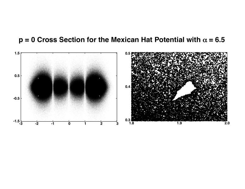
Figure 1: The $p=0$ Mexican Hat cross section for $\alpha=6.5$ has four apparent holes, one of which is shown in the closeup to the right. Here, and also in Figures 2 and 3, the abscissa is $q$ and the ordinate is the friction coefficient $\zeta$ .

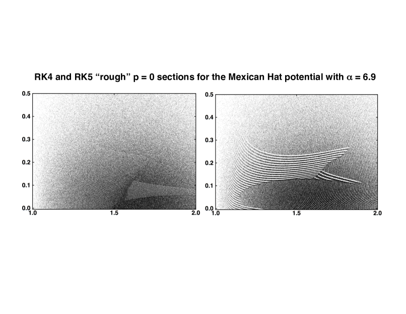
Figure 2: The $p=0$ Mexican Hat cross section closeups for $\alpha=6.9$ with the rms difference between solutions with timesteps of $dt$ and two steps of $(dt/2)$ constrained to lie in the range $10^{-14}\ {\rm to}\ 10^{-12}$. The fourth-order section is on the left and the fifth-order section is on the right.

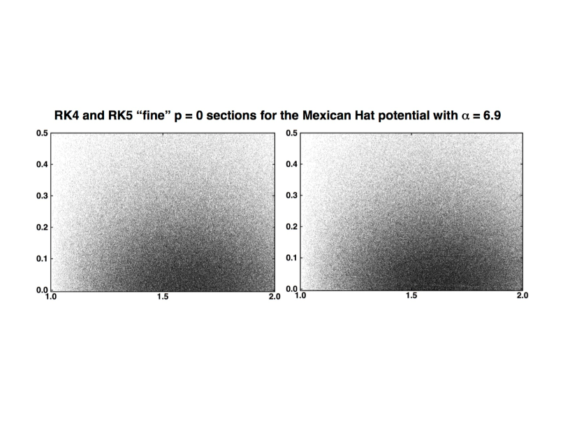
Figure 3: The $p=0$ Mexican Hat cross section closeups for $\alpha=6.9$ with the rms difference between solutions with timesteps of $dt$ and two steps of $(dt/2)$ constrained to lie in the range $10^{-17}\ {\rm to}\ 10^{-15}$. The fourth-order section is on the left and the fifth-order section is on the right.

Considerable numerical work, following the comprehensive analyses of Kusnezov, Bulgac, and Bauerb4 ; b5 , suggested that using two thermostat variables rather than one was the simplest route to oscillator ergodicity. Including another thermostat variable requires a four-dimensional $(q,p,\zeta,\xi)$ phase space. A successful exampleb6 , ergodic in $(q,p,\zeta,\xi)$ space, controlled two velocity moments, $\langle\ p^{2}\ \rangle$ and $\langle\ p^{4}\ \rangle$ rather than just one :

$$\{\ \dot{q}=p\ ;\ \dot{p}=-q-\zeta p-\xi p^{3}\ ;\ \dot{\zeta}=p^{2}-1\ ;\ \dot{\xi}=p^{4}-3p^{2}\ \}\ \longrightarrow$$

$$f(q,p,\zeta)\propto e^{-(q^{2}/2)}e^{-(p^{2}/2)}e^{-(\zeta^{2}/2)}e^{-(\xi^{2}/2)}\ [\ {\rm Hoover-Holian}\ ]\ .$$

In 2015 a single-thermostat approachb7 with simultaneous weak control of $\langle\ p^{2}\ \rangle$ and $\langle\ p^{4}\ \rangle$ was found to generate Gibbs’ entire distribution for the harmonic oscillator :

$$\{\ \dot{q}=p\ ;\ \dot{p}=-q-\zeta(0.05p+0.32p^{3})\ ;\ \dot{\zeta}=0.05(p^{2}-1)+0.32(p^{4}-3p^{2})\ \}\ .$$

Straightforward generalizations of this single-thermostat approach failed to thermostat the quartic and Mexican Hat potentials, leading to the posing of the 2016 Snook Prize problem solved by Tapias, Bravetti, and Sandersb8 .

II Tapias, Bravetti, and Sanders’ “Logistic” Thermostat

The Logistic Map and the Logistic Flow are two simple models for chaotic behavior :

$$q_{n+1}=cq_{n}(1-q_{n}){\rm\ and\ }\dot{q}=q(1-q)\ .$$

A solution of the logistic flow equation is

$$\dot{q}=\frac{1}{[\ e^{+t/2}+e^{-t/2}\ ]^{2}}\longleftrightarrow q=\frac{e^{+t/2}}{[\ e^{+t/2}+e^{-t/2}\ ]}\longleftrightarrow 2q=1+\tanh(+t/2)\ .$$

With these logistic equations in mind Tapias, Bravetti, and Sandersb8 suggested a hyperbolic tangent form for the thermostat variable, and showed, with a variety of numerical techniques, convincing evidence for the ergodicity of their “Logistic Thermostat” motion equations for the quartic and Mexican Hat potentials as well as the simpler harmonic oscillator problem.

In the most challenging case, the Mexican Hat potential, the ergodic set of motion equations found by Tapias, Bravetti, and Sanders was feasible to solve, but relatively stiff :

$$\{\ \dot{q}=p\ ;\ \dot{p}=q-q^{3}-50p\tanh(25\zeta)\ ;\ \dot{\zeta}=p^{2}-1\ \}\ .$$

In replicating their work we also characterized solutions of a slight variant :

$$\{\ \dot{q}=p\ ;\ \dot{p}=q-q^{3}-\alpha p\tanh(\alpha\zeta)\ ;\ \dot{\zeta}=p^{2}-1\ \}\ ,$$

where values of the parameter $\alpha$ in the neighborhood of seven lead to apparent ergodic behavior in $(q,p,\zeta)$ space.

One of the simplest and most useful tests for ergodicity in three dimensions is the lack of holes in the two-dimensional cross-sections (as opposed to projections) of the three-dimensional flow. For stiff equations it is convenient to use “adaptive” integrations of the motion equations where the timestep varies to maintain the accuracy of the integratorb9 .

In our own numerical work we integrated for a time of 10,000,000 using timesteps which maintained the rms difference between a fourth-order or fifth-order Runge-Kutta step of $dt$ and two such steps with $(dt/2)$ to lie within a band varying from

$$10^{-12}>\sqrt{\delta q^{2}+\delta p^{2}+\delta\zeta^{2}}>10^{-14}\ {\rm to}\ 10^{-15}>\sqrt{\delta q^{2}+\delta p^{2}+\delta\zeta^{2}}>10^{-17}\ .$$

We generated about 3,000,000 $\{\ q,0,\zeta\ \}$ double-precision cross-section points in laptop runs taking about an hour each. Typical timesteps were in the range from 0.0001 to 0.001 .

Figure 1 shows portions of the $p=0$ cross section with $\alpha=6.5$ which has evident holes at $(q=\pm 1.92,\zeta=\pm 0.39)$ . The holes disappear if $\alpha$ is increased to 6.9. But a look at the $(q,0,\zeta)$ section with an error band of $10^{-13\pm 1}$ reveals not only “normal” (irregularly-dotted) regions but also a few striped regions. In Figure 2 we see that the stripes using RK4 differ from those using RK5 showing that the stripes are artefacts. Tightening the error band to $10^{-15\pm 1}$ confirms this diagnosis, as shown in Figure 3. The interesting structure of these striped regions is a thoroughly unexpected fringe benefit of the new logistic thermostat.

We thank Drs Tapias, Bravetti, and Sanders for their stimulating prize-winning work.

References

- (1) S. Nosé, “A Unified Formulation of the Constant Temperature Molecular Dynamics Methods”, Journal of Chemical Physics 81, 511-519 (1984).
- (2) S. Nosé, “Constant Temperature Molecular Dynamics Methods”, Progress in Theoretical Physics Supplement 103, 1-46 (1991).
- (3) Wm. G. Hoover, “Canonical Dynamics: Equilibrium Phase-Space Distributions”, Physical Review A 31, 1695-1697 (1985).
- (4) D. Kusnezov, A. Bulgac, and W. Bauer, “Canonical Ensembles from Chaos”, Annals of Physics 204, 155-185 (1990).
- (5) D. Kusnezov and A. Bulgac, “Canonical Ensembles from Chaos: Constrained Dynamical Systems”, Annals of Physics 214, 180-218 (1992).
- (6) Wm. G. Hoover and B. L. Holian, “Kinetic Moments Method for the Canonical Ensemble Distribution”, Physics Letters A 211, 253-257 (1996).
- (7) Wm. G Hoover and C. G. Hoover, “Singly-Thermostated Ergodicity in Gibbs’ Canonical Ensemble and the 2016 Ian Snook Prize”, Computational Methods in Science and Technology 22, 127-131 (2016) .
- (8) D. Tapias, A. Bravetti, and D. P. Sanders, “Ergodicity of One-Dimensional Systems Coupled to the Logistic Thermostat”, Computational Methods in Science and Technology (in press, 2017) = arXiv 1611.05090 .
- (9) W. G. Hoover and C. G. Hoover, “Comparison of Very Smooth Cell-Model Trajectories Using Five Symplectic and Two Runge-Kutta Integrators”, Computational Methods in Science and Technology 21, 109-116 (2015).