Reconstruction of Scalar Potentials in $f(R,R_{\alpha\beta}R^{\alpha\beta},\phi)$ theory of gravity

Abstract

In this paper, we explore the nature of scalar field potential in $f(R,R_{\alpha\beta}R^{\alpha\beta},\phi)$ gravity using a well-motivated reconstruction scheme for flat FRW geometry. The beauty of this scheme lies in the assumption that the Hubble parameter can be expressed in terms of scalar field and vice versa. Firstly, we develop field equations in this gravity and present some general explicit forms of scalar field potential via this technique. In the first case, we take De Sitter universe model and construct some field potentials by taking different cases for coupling function. In the second case, we derive some field potentials using power law model in the presence of different matter sources like barotropic fluid, cosmological constant and Chaplygin gas for some coupling functions. From graphical analysis, it is concluded that using some specific values of the involved parameters, the reconstructed scalar field potentials are cosmologically viable in both cases.

I Introduction

The investigation about the possible causes of accelerated expansion of cosmos and nature of its missing mass and energy are some leading topics of this century. Numerous researchers are working over these lines and usually they proposed two ways to describe this accelerating expansion 1 . Some consider, general relativity (GR), as the right theory of gravity which present dark energy (DE) 2 as an easily conveyed, gradually changing cosmic fluid with negative pressure. This technique is referred as GR with modified matter sources. Other way is to modify the gravitational sector of GR 3 -6 . The $F(R)$ gravity, is one of the most attracting examples of modified gravity theories, that can be mapped into GR with extra scalar fields using an appropriate conformal transformation of metric 5 -7 . In modern cosmology, scalar fields play an important role in explaining the nature of DE 2 and to drive inflation in the beginning of universe 8 ; 9 . In literature like 10 , it is concluded that the history of cosmic expansion can be successfully discussed using scalar-tensor theories.

Many cosmological models and modified gravity theories with scalar fields, involve some general functions which cannot be derived easily from the basic theory. Then some questions frequently arise like how these particular functions should be chosen and what are physical reasons behind those particular choices. In this respect, the reconstruction technique is not a new concept, it has a long history to reconstruct the DE models. This technique allows one to find the form of scalar field potential as well as of scalar field for a specific choice of Hubble parameter in terms of scale factor or cosmic time. For a better understanding of this technique, we refer the readers to see the literature 38 .

In scalar tensor theories, it is very necessary to investigate the nature of scalar field potential and its role in explaining DE and cosmic expansion history. In 39 , the nature of scalar potential has been discussed for a minimally coupled scalar tensor theory using reconstruction technique. The reconstruction technique to explore the nature of field potentials for the models involving minimally coupling to scalar fields, two-field models and tachyon models has been given in literature 11 -28 . The reconstruction of field potentials in the models involving non-minimally coupling of scalar fields to gravity was studied in 29 -31 . Furthermore, the applications of this reconstruction technique in different gravity models and theories like the models containing non-minimally coupling of Yang-Mills fields 32 , in the framework of local 37 and nonlocal gravity 36 , in $F(R)$ and Gauss-Bonnet gravity theories 21 ; 33 ; 34 and the $F(T)$ gravity theory that involves torsion scalar $T$ as a basic ingredient 35 are available in literature.

The models of gravity that are non-minimally coupled to scalar fields are of great interest in cosmology 40 -47 . Particularly, the models having Hilbert-Einstein term in addition to the term relative to the Ricci scalar with squared scalar field were considered in quantum and inflationary cosmology 48 ; 49 . In 30 , the reconstruction process has been studied for induced gravity ($U(\phi)=\xi\phi^{2}$, where $\xi$ is an arbitrary constant). It is shown that for these cases, linearizing the differential equations to solve in reconstruction process, to derive potentials according to committed cosmological evolution. It is interesting to mention here that from this process, one can get explicit potentials which can reproduce the dynamics of flat (FRW) universe derived by different matter sources like barotropic and perfect fluids, Chaplygin gas 50 , and modified Chaplygin gas 30 .

In this regard, Kamenshchik et al. 30 has used this approach to reconstruct the field potential in terms of scalar field for FRW universe in the framework of induced gravity. They discussed this procedure for different matter distributions and concluded that the corresponding cosmic evolution can be reproduced in these cases. In 52 , the same authors used another technique known as super potential reconstruction technique for FRW model to reconstruct scalar field potentials in a non-minimally coupled scalar tensor gravity. They examined its nature for de-Sitter and barotropic models and discussed their cosmic evolution. Sharif and Waheed 53 studied the nature of scalar field potential for locally rotationally symmetric (LRS) Bianchi type I (BI) universe model in a general scalar-tensor theory via reconstruction technique and they concluded that the reconstructed potentials are viable on cosmological grounds. In a recent paper 54a , we have discussed cosmological reconstruction and energy bounds in a new general $f(R,R_{\alpha\beta}R^{\alpha\beta},\phi)$ gravity. In this gravity, we have also studied the first and second laws of black hole thermodynamics for both equilibrium and non-equilibrium descriptions 54b . Being motivated from the literature, in the present paper, we examine the nature of field potential for flat FRW universe in $f(R,R_{\alpha\beta}R^{\alpha\beta},\phi)$ gravity by applying reconstruction procedure.

This paper is arranged in the following pattern. In the next section, we give a general overview of this procedure and derive the general form of scalar field potential for this theory. In section III, we derive field potentials for de-Sitter model by taking different choices for function $f$. Section IV is devoted to explore the form of field potential for a power law model with matter sources as barotropic fluid, cosmological constant and Chaplygin gas in separate cases. In the last section, we present a summary of all sections by highlighting the major achievements.

II Basic Field Equations and General Scalar Field Potential

In this section, we present the basic formulations of the most general scalar-tensor gravity namely $f(R,R_{\alpha\beta}R^{\alpha\beta},\phi)$ theory. The gravitational action for this theory is given as follows 54 ,

$$S_{m}=\int d^{4}x\sqrt{-g}\left[\frac{1}{\kappa^{2}}\left(f\left(R,Y,\phi\right)+\omega(\phi)\phi_{;\alpha}\phi^{;\alpha}\right)+V(\phi)\right]\,,$$ (1)

where $f$ is a general function depending upon the Ricci scalar $R$, the curvature invariant $Y\equiv R_{\alpha\beta}R^{\alpha\beta}$ (where $R_{\alpha\beta}$ is the Ricci tensor) and the scalar field symbolized by $\phi$. Further, $\omega$ is a coupling function of scalar field $\phi$, the symbol $V(\phi)$ corresponds to the scalar field potential and $g$ is the determinant of metric tensor $g_{\mu\nu}$ whereas $\kappa^{2}$ represents the gravitational coupling constant.

The flat FRW spacetime with cosmic radius $a$ is given by the following metric

$$ds^{2}=dt^{2}-a^{2}(t)\left(dx^{2}+dy^{2}+dz^{2}\right)\,.$$ (2)

For which, the quantities like scalar curvature $R$ and Ricci invariant $Y$ turn out to be

$$R=-6\left(\frac{\dot{a}^{2}}{a^{2}}+\frac{\ddot{a}}{a}\right),~{}~{}~{}~{}Y=6\left(\frac{\dot{a}^{4}}{a^{4}}+\frac{2\dot{a}^{2}\ddot{a}}{a^{3}}+\frac{3\ddot{a}^{2}}{a^{2}}\right)\,,$$ (3)

while $\sqrt{-g}=a^{3}$. The Friedmann equations constructed in 54b are

$$f(R,Y,\phi)+6\left(\dot{H}+3H^{2}\right)f_{R}+6H\partial_{t}f_{R}+\omega(\phi)\dot{\phi}^{2}+V(\phi)+2\left(\dddot{H}+4H\ddot{H}+6\dot{H}H^{2}-2H^{4}\right)f_{Y}$$

$$+12H\left(3H^{2}+2\dot{H}\right)\partial_{t}f_{Y}=0\,,$$ (4)

and

$$f(R,Y,\phi)+\left(10\dot{H}+18H^{2}\right)f_{R}+4H\partial_{t}f_{R}+2\partial_{tt}f_{R}-\omega(\phi)\dot{\phi}^{2}-V(\phi)+\left(8\dddot{H}+40H\ddot{H}+20H^{2}\dot{H}\right.$$

$$\left.+32\dot{H}^{2}-36H^{4}\right)f_{Y}+8H\left(\dot{H}+3H^{2}\right)\partial_{t}f_{Y}+\left(8\dot{H}+12H^{2}\right)\partial_{tt}f_{Y}=0\,.$$ (5)

The Klein-Gordon equation is

$$2\omega(\phi)\ddot{\phi}+\frac{d\omega}{d\phi}\dot{\phi}^{2}+6H\omega(\phi)\dot{\phi}+\frac{df}{d\phi}+\frac{dV}{d\phi}=0\,.$$ (6)

From Eq. (II), we have

$$V(\phi) = -f-6\left(\dot{H}+3H^{2}\right)f_{R}-6H\partial_{t}f_{R}-2\left(3\dddot{H}+4H\ddot{H}+6H^{2}\dot{H}-2H^{4}\right)f_{Y}-12H\left(2\dot{H}\right.$$ (7)

$$\left.+3H^{2}\right)\partial_{t}f_{Y}-\omega(\phi)\dot{\phi}^{2}\,.$$

It is more appropriate to consider all the functions dependent on $``a"$ instead of cosmic time $``t"$,

$$V(\phi)=-f-6\left(3H^{2}+aHH^{\prime}\right)f_{R}+36H\left(a^{2}H^{2}H^{\prime\prime}+a^{2}H{H^{\prime}}^{2}+5aH^{2}H^{\prime}\right)f_{RR}-2\left(a^{3}H^{3}H^{\prime\prime\prime}\right.$$ (8)

$$\left.+4a^{3}H^{2}H^{\prime}H^{\prime\prime}+7a^{2}H^{3}H^{\prime\prime}+8a^{2}H^{2}{H^{\prime}}^{2}+a^{3}H{H^{\prime}}^{3}+11aH^{3}H^{\prime}-2H^{4}\right)f_{Y}-72H\left(24a^{2}H^{6}H^{\prime\prime}\right.$$

$$\left.+34a^{3}H^{5}H^{\prime}H^{\prime\prime}+96aH^{6}H^{\prime}+154a^{2}H^{5}{H^{\prime}}^{2}+78a^{3}H^{4}{H^{\prime}}^{3}+12a^{4}H^{3}{H^{\prime}}^{4}+12a^{4}H^{4}{H^{\prime}}^{2}H^{\prime\prime}\right)f_{YY}$$

$$-6aH^{2}\phi^{\prime}f_{R\phi}-12aH^{2}\phi^{\prime}\left(2aHH^{\prime}+3H^{2}\right)f_{Y\phi}-36H\left(2a^{2}H^{4}{H^{\prime\prime}}+2a^{3}H^{3}{H^{\prime}}H^{\prime\prime}+2aH^{4}H^{\prime}\right.$$

$$\left.+4a^{2}H^{3}{H^{\prime}}^{2}+2a^{3}H^{2}{H^{\prime}}^{3}\right)f_{RY}-a^{2}H^{2}\omega(\phi){\phi^{\prime}}^{2}\,.$$

By substituting the derivative of Eq. (7) in Eq. (6), we eliminate $dV/d\phi$ and the resulting equation can be written as

$$6H\ddot{\phi}f_{R\phi}+12H\left(2\dot{H}+3H^{2}\right)\ddot{\phi}f_{Y\phi}+6\left(3H^{2}+2\dot{H}\right)\dot{\phi}f_{R\phi}+2\left(\dddot{H}+16H\ddot{H}+60H^{2}\dot{H}+12\dot{H}^{2}\right.$$

$$\left.-2H^{4}\right)\dot{\phi}f_{Y\phi}-36H\left(\ddot{H}+4H\dot{H}\right)\dot{\phi}f_{RR\phi}+36H\left(2H^{2}\ddot{H}+2\dot{H}\ddot{H}\right)\dot{\phi}f_{RY\phi}+72H\left(24H^{4}\ddot{H}+34\right.$$

$$\left.\times H^{2}\dot{H}\ddot{H}+12\dot{H}^{2}\ddot{H}+96H^{3}\dot{H}^{2}+32H\dot{H}^{3}+72H^{5}\dot{H}\right)\dot{\phi}f_{YY\phi}-6H\omega(\phi)\dot{\phi}^{2}+6H\dot{\phi}^{2}f_{R\phi\phi}+12H$$

$$\times\left(2\dot{H}+3H^{2}\right)\dot{\phi}^{2}f_{Y\phi\phi}+6\left(\ddot{H}+6H\dot{H}\right)f_{R}+2\left(\ddddot{H}+4H\dddot{H}+4\dot{H}\ddot{H}+12H\dot{H}^{2}+6H^{2}\ddot{H}-8H^{3}\right.$$

$$\left.\times\dot{H}\right)f_{Y}-36\left(H\dddot{H}+4H^{2}\ddot{H}+\dot{H}\ddot{H}+8H\dot{H}^{2}\right)f_{RR}+36\left(2H^{3}\dddot{H}+2H\dot{H}\dddot{H}+6H^{2}\dot{H}\ddot{H}+2\dot{H}^{2}\ddot{H}\right.$$

$$\left.+2H\ddot{H}^{2}\right)f_{RY}+72\left(34H^{3}\dot{H}\dddot{H}+24H^{5}\dddot{H}+12H\dot{H}^{2}\dddot{H}+312H^{4}\dot{H}\ddot{H}+198H^{2}\dot{H}^{2}\ddot{H}+24H\dot{H}\ddot{H}^{2}\right.$$

$$\left.+34H^{3}\ddot{H}^{2}+12\dot{H}^{3}\ddot{H}+72H^{6}\ddot{H}+432H^{5}\dot{H}^{2}+384H^{3}\dot{H}^{3}+64H\dot{H}^{4}\right)f_{YY}=0$$ (10)

In terms of $``a"$, the above equation is written as Appendix A given in the Appendix. The field equations involve five unknowns namely $f,~{}a,~{}\phi,~{}\omega$ and $V$. Now we evaluate the scalar potential $V$ for de-Sitter and power law models (in barotropic fluid, cosmological constant and in Chaplygin gas) by taking different choices of for the remaining unknowns.

III de-Sitter Models

In cosmology, the dS-solutions are of great significance to explain the current cosmic epoch. In dS-model, the scale factor, the Hubble parameter and the Ricci tensor take the following form 55

$$a(t)=a_{0}e^{H_{0}t},~{}~{}H=H_{0},~{}~{}R=12H_{0}^{2},~{}~{}Y=36H_{0}^{4}\,.$$ (11)

Here we are using $\omega(\phi)=\omega_{0}\phi^{m}$ and $\phi(t)\sim a(t)^{\beta}$ 55 .

III.1 $f(R,Y,\phi)$ Model

We have derived the general form of $f(R,Y,\phi)$ for dS-model in 54a , here we use this form to evaluate the scalar field potential. For this model, function $f$ is defined as

$$f(R,Y,\phi)=\alpha_{1}\alpha_{2}\alpha_{3}e^{\alpha_{1}R}e^{\alpha_{2}Y}\phi^{\gamma_{1}}+\gamma_{2}\phi^{\gamma_{3}}+\gamma_{4}\phi^{\gamma_{5}}\,,$$ (12)

where $\alpha_{i}^{\prime}s$ are constants of integration and

$$\gamma_{1} = \frac{18\alpha_{1}\beta H_{0}^{2}-108\alpha_{2}\beta H_{0}^{4}-5+6\alpha_{1}H_{0}^{2}-84\alpha_{2}H_{0}^{4}}{6\left(\alpha_{1}\beta H_{0}^{2}-6\alpha_{2}\beta H_{0}^{4}\right)},~{}~{}\gamma_{2}=\omega_{0}\beta^{2}H_{0}^{2},~{}~{}\gamma_{3}=m+2,$$

$$\gamma_{4} = -2\kappa^{2}\rho_{0}a_{0}^{3(1+w)},~{}~{}\gamma_{5}=-\frac{3}{\beta}\,.$$ (13)

• Case-I:   $\omega(\phi)=\omega_{0}\phi^{m}$

Substituting model (12) into (Appendix A) and choosing $m=\gamma_{1}-2$, we have

$$\phi^{\prime\prime}+\frac{4}{3a}\left(\frac{3\alpha_{1}+4\alpha_{2}H_{0}^{2}}{\alpha_{1}+6\alpha_{2}H_{0}^{2}}\right)\phi^{\prime}+\left\{\gamma_{1}-1-\frac{\omega_{0}}{\alpha_{1}\alpha_{2}\alpha_{3}\gamma_{1}e^{\alpha_{1}R}e^{\alpha_{2}Y}\left(\alpha_{1}+6\alpha_{2}H_{0}^{2}\right)}\right\}\frac{{\phi^{\prime}}^{2}}{\phi}=0\,.$$ (14)

For the sake of simplicity, we introduce a new variable $\sigma=\phi^{\prime}/\phi$, thus (14) takes the following form:

$$\sigma^{\prime}+\frac{4}{3a}\left(\frac{3\alpha_{1}+4\alpha_{2}H_{0}^{2}}{\alpha_{1}+6\alpha_{2}H_{0}^{2}}\right)\sigma+\left\{\gamma_{1}-\frac{\omega_{0}}{\alpha_{1}\alpha_{2}\alpha_{3}\gamma_{1}e^{\alpha_{1}R}e^{\alpha_{2}Y}\left(\alpha_{1}+6\alpha_{2}H_{0}^{2}\right)}\right\}\sigma^{2}=0\,.$$ (15)

For further simplification, by introducing a new function

$$\sigma=\left\{\gamma_{1}-\frac{\omega_{0}}{\alpha_{1}\alpha_{2}\alpha_{3}\gamma_{1}e^{\alpha_{1}R}e^{\alpha_{2}Y}\left(\alpha_{1}+6\alpha_{2}H_{0}^{2}\right)}\right\}^{-1}\frac{u^{\prime}}{u}=A^{-1}\frac{u^{\prime}}{u}\,,$$ (16)

we get a differential equation for $u$ of the form:

$$u^{\prime\prime}+\frac{4\xi}{3a}u^{\prime}=0\,,$$ (17)

where $\xi=\left(\frac{3\alpha_{1}+4\alpha_{2}H_{0}^{2}}{\alpha_{1}+6\alpha_{2}H_{0}^{2}}\right)$. It is easy to see, on comparing that

$$\phi=u^{1/A}\,.$$ (18)

Equations (8) and (12) lead to the following form of scalar potential:

$$V(\phi) = -\alpha_{1}\alpha_{2}\alpha_{3}e^{\alpha_{1}R}e^{\alpha_{2}Y}\phi^{\gamma_{1}}-\gamma_{2}\phi^{\gamma_{3}}-\gamma_{4}\phi^{\gamma_{5}}-18H_{0}^{2}\alpha_{1}^{2}\alpha_{2}\alpha_{3}e^{\alpha_{1}R}e^{\alpha_{2}Y}\phi^{\gamma_{1}}-6aH_{0}^{2}\phi^{\prime}\alpha_{1}^{2}\alpha_{2}$$ (19)

$$\times \alpha_{3}\gamma_{1}e^{\alpha_{1}R}e^{\alpha_{2}Y}\phi^{\gamma_{1}-1}+4\alpha_{1}\alpha_{2}^{2}\alpha_{3}H_{0}^{4}e^{\alpha_{1}R}e^{\alpha_{2}Y}\phi^{\gamma_{1}}-36aH_{0}^{4}\phi^{\prime}\alpha_{1}\alpha_{2}^{2}\alpha_{3}\gamma_{1}e^{\alpha_{1}R}e^{\alpha_{2}Y}\phi^{\gamma_{1}-1}$$

$$- \omega_{0}a^{2}H_{0}^{2}\phi^{\gamma_{1}-2}{\phi^{\prime}}^{2}\,.$$

If $\dot{\phi}\neq 0$, all the assumptions regarding derivative of (7) are justifiable. The constant field must be discussed separately. First consider, if $\phi$ is a non-zero constant, then $f,~{}\omega$ and $V$ are also all independent of time. This leads to the cosmological evolution which is occurred due to cosmological constant. Now we can rewrite Eq.(II) as follows

$$V=-f+4H_{0}^{4}f_{Y}-18H_{0}^{2}f_{R}\,.$$ (20)

Then, on substituting $\dot{\phi}=0$ and $\dot{H}=0$ into Eq.(6), we have

$$\frac{dV}{d\phi}=-\frac{df}{d\phi}\,.$$ (21)

Multiplying Eq.(20) by Eq.(21) and then integrating, we have

$$V^{2}=\left(1-4H_{0}^{4}\alpha_{2}+18H_{0}^{2}\alpha_{1}\right)\alpha_{1}^{2}\alpha_{2}^{2}\alpha_{3}^{2}e^{24\alpha_{1}H_{0}^{2}}e^{72\alpha_{2}H_{0}^{4}}\phi^{2\gamma_{1}}+\frac{2\alpha_{1}\alpha_{2}\alpha_{3}\gamma_{2}}{\gamma_{1}+\gamma_{3}}\left(\gamma_{1}+\gamma_{3}-4H_{0}^{4}\alpha_{2}\gamma_{3}\right.$$ (22)

$$\left.+18H_{0}^{2}\alpha_{1}\gamma_{3}\right)e^{12\alpha_{1}H_{0}^{2}}e^{36\alpha_{2}H_{0}^{4}}\phi^{\gamma_{1}+\gamma_{3}}+\frac{2\alpha_{1}\alpha_{2}\alpha_{3}\gamma_{4}}{\gamma_{1}+\gamma_{5}}\left(\gamma_{1}+\gamma_{5}-4H_{0}^{4}\alpha_{2}\gamma_{5}+18H_{0}^{2}\alpha_{1}\gamma_{5}\right)e^{12\alpha_{1}H_{0}^{2}}$$

$$e^{36\alpha_{2}H_{0}^{4}}\phi^{\gamma_{1}+\gamma_{5}}+\gamma_{2}^{2}\phi^{2\gamma_{3}}+2\gamma_{2}\gamma_{4}\phi^{\gamma_{3}+\gamma_{5}}+\gamma_{4}^{2}\phi^{2\gamma_{5}}\,.$$

Now for the previous case, i.e., time dependent scalar field, the basic equation (17) is given by

$$a^{2}u^{\prime\prime}+\frac{4}{3}a\xi u^{\prime}=0\,,$$ (23)

whose general solution is

$$u(a)=c_{1}+c_{2}a^{-\xi/3}\,,$$ (24)

where $c_{1}$ and $c_{2}$ are integration constants. From (24), it can be written as

$$a=\left(\frac{c_{2}}{u-c_{1}}\right)^{3/\xi}\,,$$ (25)

and from (18), we have

$$\phi=u^{1/A}=\left(c_{1}+c_{2}a^{-\xi/3}\right)^{1/A}\,,$$ (26)

and inversely, it takes the form

$$a=\left(\frac{c_{2}}{\phi^{A}-c_{1}}\right)^{3/\xi}\,.$$ (27)

Another useful formula, in this respect, is

$$\phi^{\prime}a=-\frac{\xi}{3A}\phi\left(1-c_{1}\phi^{-A}\right)\,.$$ (28)

Inserting (26) and (28) into Eq.(19), we get

$$V(\phi)=\left(-\alpha_{1}\alpha_{2}\alpha_{3}e^{\alpha_{1}R}e^{\alpha_{2}Y}-18\alpha_{1}^{2}\alpha_{2}\alpha_{3}H_{0}^{2}e^{\alpha_{1}R}e^{\alpha_{2}Y}+\frac{2\xi}{A}\alpha_{1}^{2}\alpha_{2}\alpha_{3}\gamma_{1}H_{0}^{2}e^{\alpha_{1}R}e^{\alpha_{2}Y}+4\alpha_{1}\alpha_{2}^{2}\alpha_{3}\right.$$

$$\left.\times H_{0}^{4}e^{\alpha_{1}R}e^{\alpha_{2}Y}+\frac{12\xi}{A}\alpha_{1}\alpha_{2}^{2}\alpha_{3}\gamma_{1}H_{0}^{4}e^{\alpha_{1}R}e^{\alpha_{2}Y}-\frac{\omega_{0}\xi^{2}}{9A^{2}}H_{0}^{2}\right)\phi^{\gamma_{1}}-\gamma_{2}\phi^{\gamma_{3}}-\gamma_{4}\phi^{\gamma_{5}}+\left(\frac{2\xi c_{1}}{A}\alpha_{1}^{2}\alpha_{2}\right.$$

$$\left.\times\alpha_{3}\gamma_{1}H_{0}^{2}e^{\alpha_{1}R}e^{\alpha_{2}Y}-\frac{12\xi c_{1}}{A}\alpha_{1}\alpha_{2}^{2}\alpha_{3}\gamma_{1}H_{0}^{4}e^{\alpha_{1}R}e^{\alpha_{2}Y}+\frac{2\omega_{0}c_{1}\xi^{2}}{9A^{2}}H_{0}^{2}\right)\phi^{\gamma_{1}-A}-\frac{\omega_{0}\xi^{2}c_{1}^{2}}{9A^{2}}H_{0}^{2}\phi^{\gamma_{1}-2A}\,.$$

If we choose $c_{1}=0$ in (26), we have $\phi=c_{2}a^{-\xi/3A}$ and using this in the above equation, we get the scalar potential in terms of scale factor as follows

$$V(a)=\left(-\alpha_{1}\alpha_{2}\alpha_{3}e^{12\alpha_{1}H_{0}^{2}}e^{36\alpha_{2}H_{0}^{4}}-18\alpha_{1}^{2}\alpha_{2}\alpha_{3}H_{0}^{2}e^{12\alpha_{1}H_{0}^{2}}e^{36\alpha_{2}H_{0}^{4}}+\frac{2\xi}{A}\alpha_{1}^{2}\alpha_{2}\alpha_{3}\gamma_{1}H_{0}^{2}e^{12\alpha_{1}H_{0}^{2}}\right.$$

$$\left.e^{36\alpha_{2}H_{0}^{4}}+4\alpha_{1}\alpha_{2}^{2}\alpha_{3}H_{0}^{4}e^{12\alpha_{1}H_{0}^{2}}e^{36\alpha_{2}H_{0}^{4}}+\frac{12\xi}{A}\alpha_{1}\alpha_{2}^{2}\alpha_{3}\gamma_{1}H_{0}^{4}e^{12\alpha_{1}H_{0}^{2}}e^{36\alpha_{2}H_{0}^{4}}-\frac{\omega_{0}\xi^{2}}{9A^{2}}H_{0}^{2}\right)c_{2}^{\gamma_{1}}a^{-\xi\gamma_{1}/3A}$$

$$-\gamma_{2}c_{2}^{\gamma_{3}}a^{-\xi\gamma_{3}/3A}-\gamma_{4}c_{2}^{\gamma_{5}}a^{-\xi\gamma_{5}/3A}+\left(\frac{2\xi c_{1}}{A}\alpha_{1}^{2}\alpha_{2}\alpha_{3}\gamma_{1}H_{0}^{2}e^{12\alpha_{1}H_{0}^{2}}e^{36\alpha_{2}H_{0}^{4}}-\frac{12\xi c_{1}}{A}\alpha_{1}\alpha_{2}^{2}\alpha_{3}\gamma_{1}H_{0}^{4}\right.$$

$$\left.e^{12\alpha_{1}H_{0}^{2}}e^{36\alpha_{2}H_{0}^{4}}+\frac{2\omega_{0}c_{1}\xi^{2}}{9A^{2}}H_{0}^{2}\right)c_{2}^{\gamma_{1}-A}a^{-\xi(\gamma_{1}-A)/3A}-\frac{\omega_{0}\xi^{2}c_{1}^{2}}{9A^{2}}H_{0}^{2}c_{2}^{\gamma_{1}-2A}a^{-\xi(\gamma_{1}-2A)/3A}\,.$$ (30)

• Case-II:   $\omega(\phi)=\omega_{0}$

If we choose $\omega(\phi)=\omega_{0}$ then we have $\gamma_{1}=2,~{}\gamma_{3}=2$ and we get potential of the form

$$V(a)=\left(-\alpha_{1}\alpha_{2}\alpha_{3}e^{12\alpha_{1}H_{0}^{2}}e^{36\alpha_{2}H_{0}^{4}}-18\alpha_{1}^{2}\alpha_{2}\alpha_{3}H_{0}^{2}e^{12\alpha_{1}H_{0}^{2}}e^{36\alpha_{2}H_{0}^{4}}+\frac{4\xi}{A}\alpha_{1}^{2}\alpha_{2}\alpha_{3}H_{0}^{2}e^{12\alpha_{1}H_{0}^{2}}e^{36\alpha_{2}H_{0}^{4}}\right.$$

$$\left.+4\alpha_{1}\alpha_{2}^{2}\alpha_{3}H_{0}^{4}e^{12\alpha_{1}H_{0}^{2}}e^{36\alpha_{2}H_{0}^{4}}+\frac{24\xi}{A}\alpha_{1}\alpha_{2}^{2}\alpha_{3}H_{0}^{4}e^{12\alpha_{1}H_{0}^{2}}e^{36\alpha_{2}H_{0}^{4}}-\frac{\omega_{0}\xi^{2}}{9A^{2}}H_{0}^{2}\right)c_{2}^{2}a^{-2\xi/3A}-\gamma_{2}c_{2}^{2}\times$$

$$a^{-2\xi/3A}-\gamma_{4}c_{2}^{\gamma_{5}}a^{-\xi\gamma_{5}/3A}+\left(\frac{4\xi c_{1}}{A}\alpha_{1}^{2}\alpha_{2}\alpha_{3}H_{0}^{2}e^{12\alpha_{1}H_{0}^{2}}e^{36\alpha_{2}H_{0}^{4}}-\frac{24\xi c_{1}}{A}\alpha_{1}\alpha_{2}^{2}\alpha_{3}H_{0}^{4}e^{12\alpha_{1}H_{0}^{2}}e^{36\alpha_{2}H_{0}^{4}}\right.$$

$$\left.+\frac{2\omega_{0}c_{1}\xi^{2}}{9A^{2}}H_{0}^{2}\right)c_{2}^{2-A}a^{-\xi(2-A)/3A}-\frac{\omega_{0}\xi^{2}c_{1}^{2}}{9A^{2}}H_{0}^{2}c_{2}^{2-2A}a^{-\xi(2-2A)/3A}\,.$$ (31)

III.2 $f(R,\phi)$ Model

Now we are utilizing $f(R,\phi)$ model, independent of $Y$ which we have already constructed in the paper 54a and it is given by

$$f(R,\phi)=\alpha_{1}\alpha_{2}e^{\alpha_{1}R}\phi^{\gamma_{1}}+\gamma_{2}\phi^{\gamma_{3}}+\gamma_{4}\phi^{\gamma_{5}}\,,$$ (32)

where $\alpha_{i}^{\prime}s$ are constants of integration and

$$\gamma_{1} = -\frac{1}{\beta}(1+\frac{1}{6H_{0}^{2}\alpha_{1}}),~{}~{}\gamma_{2}=\omega_{0}\beta^{2}H_{0}^{2},~{}~{}\gamma_{3}=m+2,~{}~{}\gamma_{4}=-2\kappa^{2}\rho_{0}a_{0}^{3(1+w)},~{}~{}\gamma_{5}=-\frac{3}{\beta}\,.$$

• Case-I:   $\omega(\phi)=\omega_{0}\phi^{m}$

Substituting model (32) into (Appendix A) and choosing $m=\gamma_{1}-2$, we have

$$\phi^{\prime\prime}+\frac{4}{a}\phi^{\prime}+\left\{\gamma_{1}-1-\frac{\omega_{0}}{\alpha_{1}^{2}\alpha_{2}\gamma_{1}e^{\alpha_{1}R}}\right\}\frac{{\phi^{\prime}}^{2}}{\phi}=0\,.$$ (33)

Introducing the variable $\sigma=\phi^{\prime}/\phi$ for simplification, we can write the above equation as follows

$$\sigma^{\prime}+\frac{4}{a}\sigma+\left\{\gamma_{1}-\frac{\omega_{0}}{\alpha_{1}^{2}\alpha_{2}\gamma_{1}e^{\alpha_{1}R}}\right\}\sigma^{2}=0\,.$$ (34)

With the help of this new function

$$\sigma=\left\{\gamma_{1}-\frac{\omega_{0}}{\alpha_{1}^{2}\alpha_{2}\gamma_{1}e^{\alpha_{1}R}}\right\}^{-1}\frac{u^{\prime}}{u}=B^{-1}\frac{u^{\prime}}{u}\,,$$ (35)

we get the differential equation for $u$ in the following form

$$u^{\prime\prime}+\frac{4}{a}u^{\prime}=0\,.$$ (36)

Clearly, we have

$$\phi=u^{1/B}\,.$$ (37)

Equation (8) in case of (32) becomes

$$V(\phi) = -\alpha_{1}\alpha_{2}e^{\alpha_{1}R}\phi^{\gamma_{1}}-\gamma_{2}\phi^{\gamma_{3}}-\gamma_{4}\phi^{\gamma_{5}}-18\alpha_{1}^{2}\alpha_{2}H_{0}^{2}e^{\alpha_{1}R}\phi^{\gamma_{1}}-6a\alpha_{1}^{2}\alpha_{2}\gamma_{1}H_{0}^{2}\phi^{\prime}e^{\alpha_{1}R}\phi^{\gamma_{1}-1}$$ (38)

$$- \omega_{0}a^{2}H_{0}^{2}\phi^{\gamma_{1}-2}{\phi^{\prime}}^{2}\,.$$

If $\dot{\phi}\neq 0$, all the assumptions regarding derivative of (7) are justifiable. The constant field must be discussed separately. First consider, if $\phi$ is constant, then $f$ and $V$ are also independent of time. This leads to the cosmological evolution which is occurred due to cosmological constant. Now we can rewrite Eq. (II) as

$$V=-f-18H_{0}^{2}f_{R}\,.$$ (39)

Then, on substituting $\dot{\phi}=0$ and $\dot{H}=0$ into Eq. (6), we obtain

$$\frac{dV}{d\phi}=-\frac{df}{d\phi}\,.$$ (40)

Multiplying Eq. (39) by Eq. (40) and then by integration, we have

$$\noindent V^{2} = \left(1+18H_{0}^{2}\alpha_{1}\right)\alpha_{1}^{2}\alpha_{2}^{2}e^{24\alpha_{1}H_{0}^{2}}\phi^{2\gamma_{1}}+\frac{2\alpha_{1}\alpha_{2}\gamma_{2}}{\gamma_{1}+\gamma_{3}}\left(\gamma_{1}+\gamma_{3}+18H_{0}^{2}\alpha_{1}\gamma_{3}\right)e^{12\alpha_{1}H_{0}^{2}}\phi^{\gamma_{1}+\gamma_{3}}$$ (41)

$$+ \frac{2\alpha_{1}\alpha_{2}\gamma_{4}}{\gamma_{1}+\gamma_{5}}\left(\gamma_{1}+\gamma_{5}+18H_{0}^{2}\alpha_{1}\gamma_{5}\right)e^{12\alpha_{1}H_{0}^{2}}\phi^{\gamma_{1}+\gamma_{5}}+\gamma_{2}^{2}\phi^{2\gamma_{3}}+2\gamma_{2}\gamma_{4}\phi^{\gamma_{3}+\gamma_{5}}+\gamma_{4}^{2}\phi^{2\gamma_{5}}\,.$$

The basic equation (36) is now given by

$$a^{2}u^{\prime\prime}+4au^{\prime}=0\,,$$ (42)

whose general solution is

$$u(a)=c_{1}+c_{2}a^{-3}\,,$$ (43)

where $c_{1}$ and $c_{2}$ are integration constants. From (43), we can write

$$a=\left(\frac{c_{2}}{u-c_{1}}\right)^{1/3}\,,$$ (44)

and from (37), we have

$$\phi=u^{1/B}=\left(c_{1}+\frac{c_{2}}{a^{3}}\right)^{1/B}\,,$$ (45)

and inversely, we can write

$$a=\left(\frac{c_{2}}{\phi^{B}-c_{1}}\right)^{1/3}\,.$$ (46)

Further,

$$\phi^{\prime}a=-\frac{3}{B}\phi\left(1-c_{1}\phi^{-B}\right)\,.$$ (47)

Inserting (45) and (47) into (38), we get

$$V(\phi) = -\alpha_{1}\alpha_{2}e^{\alpha_{1}R}\phi^{\gamma_{1}}-\gamma_{2}\phi^{\gamma_{3}}-\gamma_{4}\phi^{\gamma_{5}}-18\alpha_{1}^{2}\alpha_{2}H_{0}^{2}e^{\alpha_{1}R}\phi^{\gamma_{1}}+\frac{18}{B}\alpha_{1}^{2}\alpha_{2}\gamma_{1}H_{0}^{2}e^{\alpha_{1}R}\phi^{\gamma_{1}}-\frac{9\omega_{0}}{B^{2}}H_{0}^{2}\phi^{\gamma_{1}}$$ (48)

$$- \frac{18c_{1}}{B}\alpha_{1}^{2}\alpha_{2}\gamma_{1}H_{0}^{2}e^{\alpha_{1}R}\phi^{\gamma_{1}-B}+\frac{18\omega_{0}c_{1}}{B^{2}}H_{0}^{2}\phi^{\gamma_{1}-B}-\frac{9\omega_{0}c_{1}^{2}}{B^{2}}H_{0}^{2}\phi^{\gamma_{1}-2B}\,.$$

If we choose $c_{1}=0$ in (45), we have $\phi=c_{2}a^{-3/B}$ and using it in the above equation, we get the potential in terms of scale factor as follows

$$V(\phi)=-\alpha_{1}\alpha_{2}e^{\alpha_{1}R}c_{2}^{\gamma_{2}}a^{-3\gamma_{2}/B}-\gamma_{2}c_{2}^{\gamma_{3}}a^{-3\gamma_{3}/B}-\gamma_{4}c_{2}^{\gamma_{5}}a^{-3\gamma_{5}/B}-18\alpha_{1}^{2}\alpha_{2}H_{0}^{2}e^{\alpha_{1}R}c_{2}^{\gamma_{1}}a^{-3\gamma_{1}/B}+\frac{18}{B}$$

$$\alpha_{1}^{2}\alpha_{2}\gamma_{1}H_{0}^{2}e^{\alpha_{1}R}c_{2}^{\gamma_{1}}a^{-3\gamma_{1}/B}-\frac{9\omega_{0}}{B^{2}}H_{0}^{2}c_{2}^{\gamma_{1}}a^{-3\gamma_{1}/B}-\frac{18c_{1}}{B}\alpha_{1}^{2}\alpha_{2}\gamma_{1}H_{0}^{2}e^{\alpha_{1}R}c_{2}^{\gamma_{1}-B}a^{-3(\gamma_{1}-B)/B}+\frac{18\omega_{0}c_{1}}{B^{2}}$$

$$H_{0}^{2}c_{2}^{\gamma_{1}-B}a^{-3(\gamma_{1}-B)/B}-\frac{9\omega_{0}c_{1}^{2}}{B^{2}}H_{0}^{2}c_{2}^{\gamma_{1}-2B}a^{-3(\gamma_{1}-2B)/B}\,.$$ (49)

• Case-II:   $\omega(\phi)=\omega_{0}$

If we choose $\omega(\phi)=\omega_{0}$ then we have $\gamma_{1}=2,~{}\gamma_{3}=2$ and we get potential of the form

$$V(\phi)=-\alpha_{1}\alpha_{2}e^{\alpha_{1}R}c_{2}^{\gamma_{2}}a^{-3\gamma_{2}/B}-\gamma_{2}c_{2}^{2}a^{-6/B}-\gamma_{4}c_{2}^{\gamma_{5}}a^{-3\gamma_{5}/B}-18\alpha_{1}^{2}\alpha_{2}H_{0}^{2}e^{\alpha_{1}R}c_{2}^{2}a^{-6/B}+\frac{36}{B}\alpha_{1}^{2}\alpha_{2}$$

$$H_{0}^{2}e^{\alpha_{1}R}c_{2}^{2}a^{-6/B}-\frac{9\omega_{0}}{B^{2}}H_{0}^{2}c_{2}^{2}a^{-6/B}-\frac{36c_{1}}{B}\alpha_{1}^{2}\alpha_{2}H_{0}^{2}e^{\alpha_{1}R}c_{2}^{2-B}a^{-3(2-B)/B}+\frac{18\omega_{0}c_{1}}{B^{2}}H_{0}^{2}a^{-3(2-B)/B}$$

$$\times c_{2}^{2-B}-\frac{9\omega_{0}c_{1}^{2}}{B^{2}}H_{0}^{2}c_{2}^{2-2B}a^{-3(2-2B)/B}\,.$$ (50)

III.3 $f(Y,\phi)$ Model

Here we explore the nature of field potential for $f(Y,\phi)$ model, independent of $R$ that is constructed in 54a . It has the following form

$$f(Y,\phi)=\alpha_{1}\alpha_{2}e^{\alpha_{1}Y}\phi^{\gamma_{1}}+\gamma_{2}\phi^{\gamma_{3}}+\gamma_{4}\phi^{\gamma_{5}}\,,$$ (51)

where $\alpha_{i}^{\prime}s$ are constants of integration and

$$\gamma_{1} = -\frac{7}{3\beta}+\frac{1}{36\alpha_{1}\beta H_{0}^{4}},~{}~{}\gamma_{2}=\omega_{0}\beta^{2}H_{0}^{2},~{}~{}\gamma_{3}=m+2,~{}~{}\gamma_{4}=-2\kappa^{2}\rho_{0}a_{0}^{3(1+w)},~{}~{}\gamma_{5}=-\frac{3}{\beta}\,.$$

• Case-I:   $\omega(\phi)=\omega_{0}\phi^{m}$

Substituting model (51) into (Appendix A) and choosing $m=\gamma_{1}-2$, we have

$$\phi^{\prime\prime}+\frac{8}{9a}\phi^{\prime}+\left\{\gamma_{1}-1-\frac{\omega_{0}}{6\alpha_{1}^{2}\alpha_{2}\gamma_{1}H_{0}^{2}e^{\alpha_{1}Y}}\right\}\frac{{\phi^{\prime}}^{2}}{\phi}=0\,.$$ (52)

Introducing the variable $\sigma=\phi^{\prime}/\phi$, we can write (52) as

$$\sigma^{\prime}+\frac{8}{9a}\sigma+\left\{\gamma_{1}-\frac{\omega_{0}}{6\alpha_{1}^{2}\alpha_{2}\gamma_{1}H_{0}^{2}e^{\alpha_{1}Y}}\right\}\sigma^{2}=0\,.$$ (53)

The introduction of the function

$$\sigma=\frac{\omega_{0}}{6\alpha_{1}^{2}\alpha_{2}\gamma_{1}H_{0}^{2}e^{\alpha_{1}Y}}^{-1}\frac{u^{\prime}}{u}=C^{-1}\frac{u^{\prime}}{u}\,,$$ (54)

lead to the following differential equation

$$u^{\prime\prime}+\frac{8}{9a}u^{\prime}=0\,.$$ (55)

On comparing, it is easy to check

$$\phi=u^{1/C}\,.$$ (56)

Equation (8) in case of (51) becomes

$$V(\phi) = -\alpha_{1}\alpha_{2}e^{\alpha_{1}Y}\phi^{\gamma_{1}}-\gamma_{2}\phi^{\gamma_{3}}-\gamma_{4}\phi^{\gamma_{5}}+4\alpha_{1}^{2}\alpha_{2}H_{0}^{4}e^{\alpha_{1}Y}\phi^{\gamma_{1}}-36a\alpha_{1}^{2}\alpha_{2}\gamma_{1}H_{0}^{4}\phi^{\prime}e^{\alpha_{1}Y}\phi^{\gamma_{1}-1}$$ (57)

$$- \omega_{0}a^{2}H_{0}^{2}\phi^{\gamma_{1}-2}{\phi^{\prime}}^{2}\,.$$

If $\dot{\phi}\neq 0$, all the assumptions regarding derivative of (7) are justifiable. The constant field must be discussed separately. First consider, if $\phi$ is constant, then $f$ and $V$ are also independent of time. This leads to the cosmological evolution which is occurred due to cosmological constant. Now we can rewrite Eq.(II) as

$$V=-f+4H_{0}^{4}f_{Y}\,.$$ (58)

Then, on substituting $\dot{\phi}=0$ and $\dot{H}=0$ into Eq.(6) we have

$$\frac{dV}{d\phi}=-\frac{df}{d\phi}\,.$$ (59)

Multiplying Eq.(58) by Eq.(59) and then by integration, we have

$$\noindent V^{2} = \left(1-4H_{0}^{4}\alpha_{1}\right)\alpha_{1}^{2}\alpha_{2}^{2}e^{72\alpha_{1}H_{0}^{4}}\phi^{2\gamma_{1}}+\frac{2\alpha_{1}\alpha_{2}\gamma_{2}}{\gamma_{1}+\gamma_{3}}\left(\gamma_{1}+\gamma_{3}-4H_{0}^{4}\alpha_{1}\gamma_{3}\right)e^{36\alpha_{1}H_{0}^{4}}\phi^{\gamma_{1}+\gamma_{3}}$$ (60)

$$+ \frac{2\alpha_{1}\alpha_{2}\gamma_{4}}{\gamma_{1}+\gamma_{5}}\left(\gamma_{1}+\gamma_{5}-4H_{0}^{4}\alpha_{1}\gamma_{5}\right)e^{36\alpha_{1}H_{0}^{4}}\phi^{\gamma_{1}+\gamma_{5}}+\gamma_{2}^{2}\phi^{2\gamma_{3}}+2\gamma_{2}\gamma_{4}\phi^{\gamma_{3}+\gamma_{5}}+\gamma_{4}^{2}\phi^{2\gamma_{5}}\,.$$

The basic equation (55) is now

$$a^{2}u^{\prime\prime}+\frac{8}{9}au^{\prime}=0\,,$$ (61)

whose general solution is

$$u(a)=c_{1}+c_{2}a^{1/9}\,,$$ (62)

where $c_{1}$ and $c_{2}$ are arbitrary constants. From (62), we can write

$$a=\left(\frac{u-c_{1}}{c_{2}}\right)^{9}\,,$$ (63)

and from (56), we have

$$\phi=u^{1/C}=\left(c_{1}+c_{2}a^{1/9}\right)^{1/C}\,,$$ (64)

and inversely, it can be written as

$$a=\left(\frac{\phi^{C}-c_{1}}{c_{2}}\right)^{9}\,.$$ (65)

Furthermore,

$$\phi^{\prime}a=\frac{1}{9C}\phi\left(1-c_{1}\phi^{-C}\right)\,.$$ (66)

By using (64) and (66) in Eq.(57), we get

$$V(\phi) = -\alpha_{1}\alpha_{2}e^{\alpha_{1}Y}\phi^{\gamma_{1}}-\gamma_{2}\phi^{\gamma_{3}}-\gamma_{4}\phi^{\gamma_{5}}+4\alpha_{1}^{2}\alpha_{2}H_{0}^{4}e^{\alpha_{1}Y}\phi^{\gamma_{1}}-\frac{4}{C}\alpha_{1}^{2}\alpha_{2}\gamma_{1}H_{0}^{4}e^{\alpha_{1}Y}\phi^{\gamma_{1}}-\frac{\omega_{0}}{81C^{2}}H_{0}^{2}\phi^{\gamma_{1}}$$ (67)

$$+ \frac{4c_{1}}{C}\alpha_{1}^{2}\alpha_{2}\gamma_{1}H_{0}^{4}e^{\alpha_{1}Y}\phi^{\gamma_{1}-C}+\frac{2\omega_{0}c_{1}}{81C^{2}}H_{0}^{2}\phi^{\gamma_{1}-C}-\frac{\omega_{0}c_{1}^{2}}{81C^{2}}H_{0}^{2}\phi^{\gamma_{1}-2C}\,.$$

If we choose $c_{1}=0$ in (64), we have $\phi=c_{2}a^{1/9C}$ and using it in the above equation, we get the potential in terms of scale factor as follows

$$V(a)=-\alpha_{1}\alpha_{2}e^{\alpha_{1}Y}c_{2}^{\gamma_{1}}a^{\gamma_{1}/9C}-\gamma_{2}c_{2}^{\gamma_{3}}a^{\gamma_{3}/9C}-\gamma_{4}c_{2}^{\gamma_{5}}a^{\gamma_{5}/9C}+4\alpha_{1}^{2}\alpha_{2}H_{0}^{4}e^{\alpha_{1}Y}c_{2}^{\gamma_{1}}a^{\gamma_{1}/9C}-\frac{4}{C}\alpha_{1}^{2}\alpha_{2}$$

$$\times\gamma_{1}H_{0}^{4}e^{\alpha_{1}Y}c_{2}^{\gamma_{1}}a^{\gamma_{1}/9C}-\frac{\omega_{0}}{81C^{2}}H_{0}^{2}c_{2}^{\gamma_{1}}a^{\gamma_{1}/9C}+\frac{4c_{1}}{C}\alpha_{1}^{2}\alpha_{2}\gamma_{1}H_{0}^{4}e^{\alpha_{1}Y}c_{2}^{\gamma_{1}-C}a^{\gamma_{1}-C/9C}+\frac{2\omega_{0}c_{1}}{81C^{2}}H_{0}^{2}$$

$$\times c_{2}^{\gamma_{1}-C}a^{\gamma_{1}-C/9C}-\frac{\omega_{0}c_{1}^{2}}{81C^{2}}H_{0}^{2}c_{2}^{\gamma_{1}-2C}a^{\gamma_{1}-2C/9C}\,.$$ (68)

• Case-II:   $\omega(\phi)=\omega_{0}$

If we choose $\omega(\phi)=\omega_{0}$ then we have $\gamma_{1}=2,~{}\gamma_{3}=2$ and we get potential of the form

$$V(a)=-\alpha_{1}\alpha_{2}e^{\alpha_{1}Y}c_{2}^{2}a^{2/9C}-\gamma_{2}c_{2}^{2}a^{2/9C}-\gamma_{4}c_{2}^{\gamma_{5}}a^{\gamma_{5}/9C}+4\alpha_{1}^{2}\alpha_{2}H_{0}^{4}e^{\alpha_{1}Y}c_{2}^{2}a^{2/9C}-\frac{8}{C}\alpha_{1}^{2}\alpha_{2}H_{0}^{4}e^{\alpha_{1}Y}$$

$$\times c_{2}^{2}a^{2/9C}-\frac{\omega_{0}}{81C^{2}}H_{0}^{2}c_{2}^{2}a^{2/9C}+\frac{8c_{1}}{C}\alpha_{1}^{2}\alpha_{2}H_{0}^{4}e^{\alpha_{1}Y}c_{2}^{2-C}a^{2-C/9C}+\frac{2\omega_{0}c_{1}}{81C^{2}}H_{0}^{2}c_{2}^{2-C}a^{2-C/9C}-\frac{\omega_{0}c_{1}^{2}}{81C^{2}}$$

$$\times H_{0}^{2}c_{2}^{2-2C}a^{2-2C/9C}\,.$$ (69)

We cannot discuss barotropic fluid, cosmological constant and chaplygin gas because in de-Sitter universe $H$ is constant.

IV Power-Law Models

It would be interesting to study power-law solutions in this modified gravity theory that are indicated by various eras of cosmic evolution. These solutions are helpful to clarify cosmic evolution, with the help of different epochs like dark energy, matter and radiation dominated eras. For this model, scale factor is described as 57 ; 58

$$a(t)=a_{0}t^{n},~{}~{}H(t)=\frac{n}{t},~{}~{}R=6n(1-2n)t^{-2}\,,$$ (70)

Here we are using 55

$$\omega(\phi)=\omega_{0}\phi^{m},~{}~{}\phi(t)\sim a(t)^{\beta}\,.$$ (71)

IV.1 $f(R,\phi)$ Model:

In 54a , a well-behaved model $f(R,\phi)$ has been constructed, here we are interested to evaluate the field potential using this model. The model is defined as

$$f(R,\phi)=\alpha_{1}\alpha_{2}\phi^{\gamma_{1}}R^{\gamma_{2}}+\gamma_{3}\phi^{\gamma_{4}}+\gamma_{5}\phi^{\gamma_{6}}\,,$$ (72)

where $\alpha_{i}^{\prime}s$ are constants of integration and

$$\gamma_{1} = \frac{\alpha_{1}}{3n-1}+\frac{n-3}{n\beta}-\frac{2(3n-1)^{2}}{n^{2}\beta^{2}\alpha_{1}},~{}~{}~{}\gamma_{2}=\frac{n(n-3)\beta\alpha_{1}}{(3n-1)^{2}},~{}~{}~{}\gamma_{3}=\omega_{0}\beta^{2}n^{2}a_{0}^{\frac{2}{n}},$$

$$\gamma_{4} = m+2-\frac{2}{n\beta},~{}~{}~{}\gamma_{5}=-2\kappa^{2}\rho_{0}a_{0}^{3(1+w)},~{}~{}~{}\gamma_{6}=-\frac{3}{\beta}\,.$$

Substituting model (72) into (Appendix A) and choosing $(m-\gamma_{1}+1-\frac{2}{n\beta}+\frac{2\gamma_{2}}{n\beta})=-1$, we have

$$\phi^{\prime\prime}+\frac{1}{a}\left\{\frac{4n-3}{n}-\frac{2(\gamma_{2}-1)}{n}\right\}\phi^{\prime}+\bigg{\{}\gamma_{1}-1-\frac{\omega_{0}(6n-12n^{2})^{1-\gamma_{2}}a_{0}^{(2-2\gamma_{2})/n}}{\alpha_{1}\alpha_{2}\gamma_{1}\gamma_{2}}\bigg{\}}\frac{{\phi^{\prime}}^{2}}{\phi}$$

$$+\frac{1}{a^{2}}\left\{\frac{2-6n}{n^{2}\gamma_{1}}+\frac{8(\gamma_{2}-1)}{n^{2}\gamma_{1}}\right\}\phi=0\,.$$ (73)

Introducing the variable $\sigma=\phi^{\prime}/\phi$, we can write (IV.1) as

$$\sigma^{\prime}+\frac{1}{a}\left\{\frac{4n-3}{n}-\frac{2(\gamma_{2}-1)}{n}\right\}\sigma+\bigg{\{}\gamma_{1}-\frac{\omega_{0}(6n-12n^{2})^{1-\gamma_{2}}a_{0}^{(2-2\gamma_{2})/n}}{\alpha_{1}\alpha_{2}\gamma_{1}\gamma_{2}}\bigg{\}}\sigma^{2}$$

$$+\frac{1}{a^{2}}\left\{\frac{2-6n}{n^{2}\gamma_{1}}+\frac{8(\gamma_{2}-1)}{n^{2}\gamma_{1}}\right\}=0\,.$$ (74)

On introducing a new function

$$\sigma=\bigg{\{}\gamma_{1}-\frac{\omega_{0}(6n-12n^{2})^{1-\gamma_{2}}a_{0}^{(2-2\gamma_{2})/n}}{\alpha_{1}\alpha_{2}\gamma_{1}\gamma_{2}}\bigg{\}}^{-1}\frac{u^{\prime}}{u}=D^{-1}\frac{u^{\prime}}{u}\,,$$ (75)

we get differential equation of the form

$$u^{\prime\prime}+\frac{\xi}{a}u^{\prime}+\frac{D\eta}{a^{2}}u=0\,,$$ (76)

where

$$D=\bigg{\{}\gamma_{1}-\frac{\omega_{0}(6n-12n^{2})^{1-\gamma_{2}}a_{0}^{(2-2\gamma_{2})/n}}{\alpha_{1}\alpha_{2}\gamma_{1}\gamma_{2}}\bigg{\}},~{}~{}\eta=\left\{\frac{2-6n}{n^{2}\gamma_{1}}+\frac{8(\gamma_{2}-1)}{n^{2}\gamma_{1}}\right\}$$

$$\xi=\left\{\frac{4n-3}{n}-\frac{2(\gamma_{2}-1)}{n}\right\}\,.$$ (77)

On comparison, we have

$$\phi=u^{1/D}\,.$$ (78)

Eq.(8) in case of (72) becomes

$$V(\phi) = -\alpha_{1}\alpha_{2}\phi^{\gamma_{1}}R^{\gamma_{2}}-\gamma_{3}\phi^{\gamma_{4}}-\gamma_{5}\phi^{\gamma_{6}}-6\alpha_{1}\alpha_{2}\gamma_{2}(3H^{2}+aHH^{\prime})\phi^{\gamma_{1}}R^{\gamma_{2}-1}+36\alpha_{1}\alpha_{2}\gamma_{2}(\gamma_{2}-1)$$ (79)

$$\times H\left(a^{2}H^{2}H^{\prime\prime}+a^{2}H{H^{\prime}}^{2}+5aH^{2}H^{\prime}\right)\phi^{\gamma_{1}}R^{\gamma_{2}-2}-6a\alpha_{1}\alpha_{2}\gamma_{1}\gamma_{2}H^{2}\phi^{\prime}\phi^{\gamma_{1}-1}R^{\gamma_{2}-1}$$

$$- \omega_{0}a^{2}H^{2}\phi^{m}{\phi^{\prime}}^{2}\,.$$

If $\dot{\phi}\neq 0$, all the assumptions regarding derivative of (7) are justifiable. The constant field must be discussed separately. First consider, if $\phi$ is constant, then $f$ and $V$ are also independent of time and from Friedmann equation (II), it can be noticed that the Hubble parameter $H$ is also a constant. This leads to the cosmological evolution which is occurred due to cosmological constant. Now we can rewrite Eq.(II) as follows

$$V=-f-18H^{2}f_{R}\,.$$ (80)

Then, on substituting $\dot{\phi}=0$ and $\dot{H}=0$ into Eq.(6), we have

$$\frac{dV}{d\phi}=-\frac{df}{d\phi}\,.$$ (81)

Multiplying equations (80), (81) and substituting model (72), and then by integrating, we have the potential in this form

$$V^{2} = \frac{n\beta\alpha_{1}^{2}\alpha_{2}^{2}\gamma_{1}}{n\beta\gamma_{1}-2\gamma_{2}}\left(R+18H^{2}\gamma_{2}\right)R^{2\gamma_{2}-1}\phi^{2\gamma_{1}}+\frac{2n\beta\alpha_{1}\alpha_{2}\gamma_{3}}{(\gamma_{1}+\gamma_{4})n\beta-2\gamma_{2}}\left(\gamma_{1}R+\gamma_{4}R+18H^{2}\gamma_{2}\gamma_{4}\right)R^{\gamma_{2}-1}$$ (82)

$$\times \phi^{\gamma_{1}+\gamma_{4}}+\frac{2n\beta\alpha_{1}\alpha_{2}\gamma_{5}}{(\gamma_{1}+\gamma_{6})n\beta-2\gamma_{2}}\left(\gamma_{1}R+\gamma_{6}R+18H^{2}\gamma_{2}\gamma_{6}\right)R^{\gamma_{2}-1}\phi^{\gamma_{1}+\gamma_{6}}+\gamma_{3}^{2}\phi^{2\gamma_{4}}+2\gamma_{3}\gamma_{5}\phi^{\gamma_{4}+\gamma_{6}}$$

$$+ \gamma_{5}^{2}\phi^{2\gamma_{6}}$$

IV.1.1 Barotropic Fluid

Equation of state parameter for barotropic fluid is

$$p=w\rho\,,$$ (83)

and Hubble parameter defined as

$$H(a)=H_{0}a^{-\frac{3}{2}(1+w)}\,.$$ (84)

The basic equation (76) is now

$$a^{2}u^{\prime\prime}+a\xi u^{\prime}+D\eta u=0\,,$$ (85)

whose general solution is

$$u(a)=c_{1}a^{p_{1}}+c_{2}a^{p_{2}}\,,$$ (86)

where $c_{1}$ and $c_{2}$ are integration constants, and the exponents $p_{1}$ and $p_{2}$ are

$$p_{1,2}=\left(\frac{1-\xi}{2}\right)\pm\sqrt{\left(\frac{1-\xi}{2}\right)^{2}-D\eta}\,.$$ (87)

For the sake of simplicity, we choose one of the constants $c_{1}$ or $c_{2}$ as zero. In this situation, one can hope to modify the function (86). For this choice, we have

$$a=u^{1/p_{1,2}}\,,$$ (88)

and from (78), we have

$$\phi=u^{1/D}=a^{\frac{p_{1,2}}{D}}\,,$$ (89)

and inversely, we can write

$$a=\phi^{D/p_{1,2}}\,.$$ (90)

Furthermore,

$$\phi^{\prime}a=\frac{p_{1,2}}{D}\phi\,,$$ (91)

• Case-I:   $\omega(\phi)=\omega_{0}\phi^{m}$

Inserting (84), (89) and (91) into Eq.(79), we have

$$V_{1,2} = -\alpha_{1}\alpha_{2}{3}^{\gamma_{2}}H_{0}^{2\gamma_{2}}(3w-1)^{\gamma_{2}}\phi^{\gamma_{1}-\frac{3(1+w)\gamma_{2}D}{p_{1,2}}}-\gamma_{3}\phi^{\gamma_{4}}-\gamma_{5}\phi^{\gamma_{6}}-3^{\gamma_{2}+1}\alpha_{1}\alpha_{2}\gamma_{2}H_{0}^{2\gamma_{2}}(3w-1)^{\gamma_{2}-1}$$ (92)

$$\times (1-w)\phi^{\gamma_{1}-\frac{3(1+w)\gamma_{2}D}{p_{1,2}}}+18\alpha_{1}\alpha_{2}\gamma_{2}(\gamma_{2}-1)3^{\gamma_{2}}(1+w)^{2}(3w-1)^{\gamma_{2}-2}H_{0}^{2\gamma_{2}}\phi^{\gamma_{1}-\frac{3(1+w)\gamma_{2}D}{p_{1,2}}}$$

$$- \frac{2p_{1,2}}{D}\alpha_{1}\alpha_{2}\gamma_{1}\gamma_{2}3^{\gamma_{2}}H_{0}^{2\gamma_{2}}(3w-1)^{\gamma_{2}-1}\phi^{\gamma_{1}-\frac{3(1+w)\gamma_{2}D}{p_{1,2}}}-\frac{\omega_{0}p_{1,2}^{2}}{D^{2}}H_{0}^{2}\phi^{m+2-\frac{3(1+w)D}{p_{1,2}}}\,.$$

Using (89) in the above equation, we get the scalar potential in terms of scale factor as follows

$$V_{1,2}=-\alpha_{1}\alpha_{2}{3}^{\gamma_{2}}H_{0}^{2\gamma_{2}}(3w-1)^{\gamma_{2}}a^{\xi_{1}}-\gamma_{3}\phi^{\gamma_{4}}-\gamma_{5}\phi^{\gamma_{6}}-3^{\gamma_{2}+1}\alpha_{1}\alpha_{2}\gamma_{2}H_{0}^{2\gamma_{2}}(3w-1)^{\gamma_{2}-1}(1-w)a^{\xi_{1}}$$

$$+18\alpha_{1}\alpha_{2}\gamma_{2}(\gamma_{2}-1)3^{\gamma_{2}}(1+w)^{2}(3w-1)^{\gamma_{2}-2}H_{0}^{2\gamma_{2}}a^{\xi_{1}}-\frac{2p_{1,2}}{D}\alpha_{1}\alpha_{2}\gamma_{1}\gamma_{2}3^{\gamma_{2}}H_{0}^{2\gamma_{2}}(3w-1)^{\gamma_{2}-1}a^{\xi_{1}}$$

$$-\frac{\omega_{0}p_{1,2}^{2}}{D^{2}}H_{0}^{2}a^{\xi_{2}}\,,$$ (93)

where $\xi_{1}=-3(1+w)\gamma_{2}+\frac{\gamma_{1}p_{1,2}}{D}$ and $\xi_{2}=-3(1+w)+\frac{(m+2)p_{1,2}}{D}$.

• Case-II:   $\omega(\phi)=\omega_{0}$

If we choose $\omega(\phi)=\omega_{0}$ then we have $\gamma_{1}+\frac{2}{n\beta}-\frac{2\gamma_{2}}{n\beta}=2,~{}\gamma_{4}=2-\frac{2}{n\beta}$ and potential is of the form

$$V_{1,2}=-\alpha_{1}\alpha_{2}{3}^{\gamma_{2}}H_{0}^{2\gamma_{2}}(3w-1)^{\gamma_{2}}a^{\xi_{1}}-\gamma_{3}\phi^{\gamma_{4}}-\gamma_{5}\phi^{\gamma_{6}}-3^{\gamma_{2}+1}\alpha_{1}\alpha_{2}\gamma_{2}H_{0}^{2\gamma_{2}}(3w-1)^{\gamma_{2}-1}(1-w)a^{\xi_{1}}$$

$$+18\alpha_{1}\alpha_{2}\gamma_{2}(\gamma_{2}-1)3^{\gamma_{2}}(1+w)^{2}(3w-1)^{\gamma_{2}-2}H_{0}^{2\gamma_{2}}a^{\xi_{1}}-\frac{2p_{1,2}}{D}\alpha_{1}\alpha_{2}\gamma_{1}\gamma_{2}3^{\gamma_{2}}H_{0}^{2\gamma_{2}}(3w-1)^{\gamma_{2}-1}a^{\xi_{1}}$$

$$-\frac{\omega_{0}p_{1,2}^{2}}{D^{2}}H_{0}^{2}a^{\xi_{2}}\,.$$ (94)

where $\xi_{1}=-3(1+w)\gamma_{2}+\frac{\gamma_{1}p_{1,2}}{D}$ and $\xi_{2}=-3(1+w)+\frac{2p_{1,2}}{D}$.

IV.1.2 Cosmological Constant

• Case-I:   $\omega(\phi)=\omega_{0}\phi^{m}$

If $w=-1$ then we have

$$H=H_{0},~{}~{}R=12H_{0}^{2}\,$$

and consequently Eq.(92) transforms to

$$V_{1,2}(\phi) = -\alpha_{1}\alpha_{2}(12)^{\gamma_{2}}H_{0}^{2\gamma_{2}}\phi^{\gamma_{1}}-\gamma_{3}\phi^{\gamma_{4}}-\gamma_{5}\phi^{\gamma_{6}}-18\alpha_{1}\alpha_{2}\gamma_{2}(12)^{\gamma_{2}-1}H_{0}^{2\gamma_{2}}\phi^{\gamma_{1}}-\frac{p_{1,2}}{2D}\alpha_{1}\alpha_{2}\gamma_{1}\gamma_{2}$$ (95)

$$\times (12)^{\gamma_{2}}H_{0}^{2\gamma_{2}}\phi^{\gamma_{1}}-\frac{\omega_{0}p_{1,2}^{2}}{D^{2}}H_{0}^{2}\phi^{m+2}\,.$$

In terms of scale factor, the above equation can be written as

$$V_{1,2}(a) = -\alpha_{1}\alpha_{2}(12)^{\gamma_{2}}H_{0}^{2\gamma_{2}}a^{\frac{\gamma_{1}p_{1,2}}{D}}-\gamma_{3}a^{\frac{\gamma_{4}p_{1,2}}{D}}-\gamma_{5}a^{\frac{\gamma_{6}p_{1,2}}{D}}-18\alpha_{1}\alpha_{2}\gamma_{2}(12)^{\gamma_{2}-1}H_{0}^{2\gamma_{2}}a^{\frac{\gamma_{1}p_{1,2}}{D}}-\frac{p_{1,2}}{2D}$$ (96)

$$\times \alpha_{1}\alpha_{2}\gamma_{1}\gamma_{2}(12)^{\gamma_{2}}H_{0}^{2\gamma_{2}}a^{\frac{\gamma_{1}p_{1,2}}{D}}-\frac{\omega_{0}p_{1,2}^{2}}{D^{2}}H_{0}^{2}a^{(m+2)p_{1,2}/D}\,.$$

• Case-II:   $\omega(\phi)=\omega_{0}$

For constant coupling, we have $m=0$ then $\gamma_{1}+\frac{2}{n\beta}-\frac{2\gamma_{2}}{n\beta}=2,~{}\gamma_{4}=2-\frac{2}{n\beta}$ and then potential takes the form

$$V_{1,2}(a) = -\alpha_{1}\alpha_{2}(12)^{\gamma_{2}}H_{0}^{2\gamma_{2}}a^{\frac{\gamma_{1}p_{1,2}}{D}}-\gamma_{3}a^{\frac{\gamma_{4}p_{1,2}}{D}}-\gamma_{5}a^{\frac{\gamma_{6}p_{1,2}}{D}}-18\alpha_{1}\alpha_{2}\gamma_{2}(12)^{\gamma_{2}-1}H_{0}^{2\gamma_{2}}a^{\frac{\gamma_{1}p_{1,2}}{D}}-\frac{p_{1,2}}{2D}$$ (97)

$$\times \alpha_{1}\alpha_{2}\gamma_{1}\gamma_{2}(12)^{\gamma_{2}}H_{0}^{2\gamma_{2}}a^{\frac{\gamma_{1}p_{1,2}}{D}}-\frac{\omega_{0}p_{1,2}^{2}}{D^{2}}H_{0}^{2}a^{2p_{1,2}/D}\,.$$

IV.1.3 Chaplygin Gas

The Chaplygin gas model 50 is one of the basic model of dark energy and dark matter that has gained a certain recognition 50 ; 60 ; 61 . For Chaplygin gas, the equation of state is

$$p=\frac{\hat{A}}{\rho}\,,$$ (98)

with Hubble parameter of the form

$$H(a)=\left(\hat{A}+\frac{\hat{B}}{a^{6}}\right)^{1/4}\,,$$ (99)

where $\hat{A}$ is a constant.

• Case-I:   $\omega(\phi)=\omega_{0}\phi^{m}$

Using Eq.(99), the equation (79) takes the form

$$V_{1,2}=-\alpha_{1}\alpha_{2}(-6)^{\gamma_{2}}\left(\hat{A}+\frac{\hat{B}}{a^{6}}\right)^{-\frac{1}{2}\gamma_{2}}\left(2\hat{A}+\frac{\hat{B}}{2a^{6}}\right)^{\gamma_{2}}\phi^{\gamma_{1}}-\gamma_{3}\phi^{\gamma_{4}}-\gamma_{5}\phi^{\gamma_{6}}+\alpha_{1}\alpha_{2}\gamma_{2}(-6)^{\gamma_{2}}$$

$$\left(\hat{A}+\frac{\hat{B}}{a^{6}}\right)^{-\frac{1}{2}\gamma_{2}}\left(2\hat{A}+\frac{\hat{B}}{2a^{6}}\right)^{\gamma_{2}-1}\left(3\hat{A}+\frac{3\hat{B}}{2a^{6}}\right)\phi^{\gamma_{1}}+\alpha_{1}\alpha_{2}\gamma_{2}(\gamma_{2}-1)(-6)^{\gamma_{2}}\left(\hat{A}+\frac{\hat{B}}{a^{6}}\right)^{-\frac{1}{2}\gamma_{2}}$$

$$\left(2\hat{A}+\frac{\hat{B}}{2a^{6}}\right)^{\gamma_{2}-2}\left(\frac{3\hat{A}\hat{B}}{a^{6}}-\frac{3\hat{B}^{2}}{2a^{12}}\right)\phi^{\gamma_{1}}+\frac{p_{1,2}}{D}\alpha_{1}\alpha_{2}\gamma_{1}\gamma_{2}(-6)^{\gamma_{2}}\left(\hat{A}+\frac{\hat{B}}{a^{6}}\right)^{1-\frac{1}{2}\gamma_{2}}\left(2\hat{A}+\frac{\hat{B}}{2a^{6}}\right)^{\gamma_{2}-1}$$

$$-\frac{\omega_{0}p_{1,2}^{2}}{D^{2}}\left(\hat{A}+\frac{\hat{B}}{a^{6}}\right)^{1/2}\phi^{m+2}\,.$$ (100)

In terms of scale factor, the potential for Chaplygin gas is defined by

$$V_{1,2}(a)=-\alpha_{1}\alpha_{2}(-6)^{\gamma_{2}}\left(\hat{A}+\frac{\hat{B}}{a^{6}}\right)^{-\frac{1}{2}\gamma_{2}}\left(2\hat{A}+\frac{\hat{B}}{2a^{6}}\right)^{\gamma_{2}}a^{\frac{\gamma_{1}p_{1,2}}{D}}-\gamma_{3}a^{\frac{\gamma_{4}p_{1,2}}{D}}-\gamma_{5}a^{\frac{\gamma_{6}p_{1,2}}{D}}+\alpha_{1}\alpha_{2}\gamma_{2}$$

$$(-6)^{\gamma_{2}}\left(\hat{A}+\frac{\hat{B}}{a^{6}}\right)^{-\frac{1}{2}\gamma_{2}}\left(2\hat{A}+\frac{\hat{B}}{2a^{6}}\right)^{\gamma_{2}-1}\left(3\hat{A}+\frac{3\hat{B}}{2a^{6}}\right)a^{\frac{\gamma_{1}p_{1,2}}{D}}+\alpha_{1}\alpha_{2}\gamma_{2}(\gamma_{2}-1)\left(\hat{A}+\frac{\hat{B}}{a^{6}}\right)^{-\frac{1}{2}\gamma_{2}}$$

$$(-6)^{\gamma_{2}}\left(2\hat{A}+\frac{\hat{B}}{2a^{6}}\right)^{\gamma_{2}-2}\left(\frac{3\hat{A}\hat{B}}{a^{6}}-\frac{3\hat{B}^{2}}{2a^{12}}\right)a^{\frac{\gamma_{1}p_{1,2}}{D}}+\frac{p_{1,2}}{D}\alpha_{1}\alpha_{2}\gamma_{1}\gamma_{2}(-6)^{\gamma_{2}}\left(\hat{A}+\frac{\hat{B}}{a^{6}}\right)^{1-\frac{1}{2}\gamma_{2}}$$

$$\left(2\hat{A}+\frac{\hat{B}}{2a^{6}}\right)^{\gamma_{2}-1}-\frac{\omega_{0}p_{1,2}^{2}}{D^{2}}\left(\hat{A}+\frac{\hat{B}}{a^{6}}\right)^{1/2}a^{\frac{(m+2)p_{1,2}}{D}}\,.$$ (101)

• Case-II:   $\omega(\phi)=\omega_{0}$

For $m=0$, i.e., constant coupling, we have $\gamma_{1}+\frac{2}{n\beta}-\frac{2\gamma_{2}}{n\beta}=2,~{}\gamma_{4}=2-\frac{2}{n\beta}$ and thus potential of the following form

$$V_{1,2}(a)=-\alpha_{1}\alpha_{2}(-6)^{\gamma_{2}}\left(\hat{A}+\frac{\hat{B}}{a^{6}}\right)^{-\frac{1}{2}\gamma_{2}}\left(2\hat{A}+\frac{\hat{B}}{2a^{6}}\right)^{\gamma_{2}}a^{\frac{\gamma_{1}p_{1,2}}{D}}-\gamma_{3}a^{\frac{\gamma_{4}p_{1,2}}{D}}-\gamma_{5}a^{\frac{\gamma_{6}p_{1,2}}{D}}+\alpha_{1}\alpha_{2}\gamma_{2}$$

$$(-6)^{\gamma_{2}}\left(\hat{A}+\frac{\hat{B}}{a^{6}}\right)^{-\frac{1}{2}\gamma_{2}}\left(2\hat{A}+\frac{\hat{B}}{2a^{6}}\right)^{\gamma_{2}-1}\left(3\hat{A}+\frac{3\hat{B}}{2a^{6}}\right)a^{\frac{\gamma_{1}p_{1,2}}{D}}+\alpha_{1}\alpha_{2}\gamma_{2}(\gamma_{2}-1)\left(\hat{A}+\frac{\hat{B}}{a^{6}}\right)^{-\frac{1}{2}\gamma_{2}}$$

$$(-6)^{\gamma_{2}}\left(2\hat{A}+\frac{\hat{B}}{2a^{6}}\right)^{\gamma_{2}-2}\left(\frac{3\hat{A}\hat{B}}{a^{6}}-\frac{3\hat{B}^{2}}{2a^{12}}\right)a^{\frac{\gamma_{1}p_{1,2}}{D}}+\frac{p_{1,2}}{D}\alpha_{1}\alpha_{2}\gamma_{1}\gamma_{2}(-6)^{\gamma_{2}}\left(\hat{A}+\frac{\hat{B}}{a^{6}}\right)^{1-\frac{1}{2}\gamma_{2}}$$

$$\left(2\hat{A}+\frac{\hat{B}}{2a^{6}}\right)^{\gamma_{2}-1}-\frac{\omega_{0}p_{1,2}^{2}}{D^{2}}\left(\hat{A}+\frac{\hat{B}}{a^{6}}\right)^{1/2}a^{\frac{2p_{1,2}}{D}}\,.$$ (102)

IV.2 $f(Y,\phi)$ Model

Here we use $f(Y,\phi)$ model that is constructed in a recent paper 54a . The model is described as

$$f(Y,\phi)=\alpha_{1}\alpha_{2}\phi^{\gamma_{1}}Y^{\gamma_{2}}+\gamma_{3}\phi^{\gamma_{4}}+\gamma_{5}\phi^{\gamma_{6}}\,,$$ (103)

where $\alpha_{i}^{\prime}s$ are constants of integration and

$$\gamma_{1} = \frac{2(3n-2)\alpha_{1}}{4n^{2}-3n+1}+\frac{7n^{2}-31n+12}{n(3n-2)}-\frac{2(4n^{2}-3n+1)^{2}}{n^{2}(3n-2)^{2}\alpha_{1}},~{}~{}~{}\gamma_{2}=\frac{n(3n-2)\alpha_{1}}{2(4n^{2}-3n+1)},$$

$$\gamma_{3} = -\omega_{0}\beta^{2}n^{2}a_{0}^{\frac{2}{n}},~{}~{}~{}\gamma_{4}=m+2-\frac{2}{n\beta},~{}~{}~{}\gamma_{5}=-2\kappa^{2}\rho_{0}a_{0}^{3(1+w)},~{}~{}~{}\gamma_{6}=-\frac{3}{\beta}\,.$$

Substituting model (103) into (Appendix A) and choosing $(m-\gamma_{1}+1-\frac{2}{n\beta}+\frac{4\gamma_{2}}{n\beta})=-1$, we have

$$\phi^{\prime\prime}+\frac{1}{a}\left\{\frac{32n^{3}-180n^{2}+112n-12}{12n^{2}(3n-2)}-\frac{(\gamma_{2}-1)(72n^{3}-144n^{2}+100n-24)}{n(3n-2)(6n^{2}-8n+3)}\right\}\phi^{\prime}$$

$$+\bigg{\{}\gamma_{1}-1-\frac{\omega_{0}(6)^{1-\gamma_{2}}n^{1-2\gamma_{2}}a_{0}^{(2-4\gamma_{2})/n}(6n^{2}-8n+3)^{1-\gamma_{2}}}{2(3n-2)\alpha_{1}\alpha_{2}\gamma_{1}\gamma_{2}}\bigg{\}}\frac{{\phi^{\prime}}^{2}}{\phi}+\frac{1}{a^{2}}\bigg{\{}\frac{24-32n+24n^{2}+8n^{3}}{6n^{3}\gamma_{1}(3n-2)}$$

$$+\frac{(\gamma_{2}-1)(610n^{3}-1152n^{2}+800n-192)}{n^{2}\gamma_{1}(3n-2)(6n^{2}-8n+3)}\bigg{\}}\phi=0\,.$$ (104)

Introducing the variable $\sigma=\phi^{\prime}/\phi$, we can write (IV.2) as

$$\sigma^{\prime}+\frac{1}{a}\left\{\frac{32n^{3}-180n^{2}+112n-12}{12n^{2}(3n-2)}-\frac{(\gamma_{2}-1)(72n^{3}-144n^{2}+100n-24)}{n(3n-2)(6n^{2}-8n+3)}\right\}\sigma$$

$$+\bigg{\{}\gamma_{1}-\frac{\omega_{0}(6)^{1-\gamma_{2}}n^{1-2\gamma_{2}}a_{0}^{(2-4\gamma_{2})/n}(6n^{2}-8n+3)^{1-\gamma_{2}}}{2(3n-2)\alpha_{1}\alpha_{2}\gamma_{1}\gamma_{2}}\bigg{\}}\sigma^{2}+\frac{1}{a^{2}}\bigg{\{}\frac{24-32n+24n^{2}+8n^{3}}{6n^{3}\gamma_{1}(3n-2)}$$

$$+\frac{(\gamma_{2}-1)(610n^{3}-1152n^{2}+800n-192)}{n^{2}\gamma_{1}(3n-2)(6n^{2}-8n+3)}\bigg{\}}\phi=0\,.$$ (105)

On introducing a new function

$$\sigma=\bigg{\{}\gamma_{1}-\frac{\omega_{0}(6)^{1-\gamma_{2}}n^{1-2\gamma_{2}}a_{0}^{(2-4\gamma_{2})/n}(6n^{2}-8n+3)^{1-\gamma_{2}}}{2(3n-2)\alpha_{1}\alpha_{2}\gamma_{1}\gamma_{2}}\bigg{\}}^{-1}\frac{u^{\prime}}{u}=E^{-1}\frac{u^{\prime}}{u}\,,$$ (106)

we get differential equation of the form

$$u^{\prime\prime}+\frac{\xi}{a}u^{\prime}+\frac{E\eta}{a^{2}}u=0\,,$$ (107)

where

$$E=\bigg{\{}\gamma_{1}-\frac{\omega_{0}(6)^{1-\gamma_{2}}n^{1-2\gamma_{2}}a_{0}^{(2-4\gamma_{2})/n}(6n^{2}-8n+3)^{1-\gamma_{2}}}{2(3n-2)\alpha_{1}\alpha_{2}\gamma_{1}\gamma_{2}}\bigg{\}},$$

$$\xi=\left\{\frac{32n^{3}-180n^{2}+112n-12}{12n^{2}(3n-2)}-\frac{(\gamma_{2}-1)(72n^{3}-144n^{2}+100n-24)}{n(3n-2)(6n^{2}-8n+3)}\right\}$$

$$\eta=\bigg{\{}\frac{24-32n+24n^{2}+8n^{3}}{6n^{3}\gamma_{1}(3n-2)}+\frac{(\gamma_{2}-1)(610n^{3}-1152n^{2}+800n-192)}{n^{2}\gamma_{1}(3n-2)(6n^{2}-8n+3)}\bigg{\}}\,.$$ (108)

It is easy to see, on comparing that

$$\phi=u^{1/E}\,.$$ (109)

Equation (8) in case of (103) becomes

$$V(\phi)=-\alpha_{1}\alpha_{2}\phi^{\gamma_{1}}Y^{\gamma_{2}}-\gamma_{3}\phi^{\gamma_{4}}-\gamma_{5}\phi^{\gamma_{6}}-2\left(a^{3}H^{3}H^{\prime\prime\prime}+4a^{3}H^{2}H^{\prime}H^{\prime\prime}+7a^{2}H^{3}H^{\prime\prime}+8a^{2}H^{2}{H^{\prime}}^{2}\right.$$

$$\left.+a^{3}H{H^{\prime}}^{3}+11aH^{3}H^{\prime}-2H^{4}\right)\alpha_{1}\alpha_{2}\gamma_{2}\phi^{\gamma_{1}}Y^{\gamma_{2}-1}-72H\left(24a^{2}H^{6}H^{\prime\prime}+34a^{3}H^{5}H^{\prime}H^{\prime\prime}+96aH^{6}H^{\prime}\right.$$

$$\left.+154a^{2}H^{5}{H^{\prime}}^{2}+78a^{3}H^{4}{H^{\prime}}^{3}+12a^{4}H^{3}{H^{\prime}}^{4}+12a^{4}H^{4}{H^{\prime}}^{2}H^{\prime\prime}\right)\alpha_{1}\alpha_{2}\gamma_{2}(\gamma_{2}-1)\phi^{\gamma_{1}}Y^{\gamma_{2}-2}-12aH^{2}$$

$$\times\phi^{\prime}\left(2aHH^{\prime}+3H^{2}\right)\alpha_{1}\alpha_{2}\gamma_{1}\gamma_{2}\phi^{\gamma_{1}}Y^{\gamma_{2}-1}-\omega_{0}a^{2}H^{2}\phi^{m}{\phi^{\prime}}^{2}\,.$$ (110)

If $\dot{\phi}\neq 0$, all the assumptions regarding derivative of (7) are justifiable. The constant field must be discussed separately. First consider, if $\phi$ is constant, then $f$ and $V$ are also independent of time and from Friedmann equation (II), it can be noticed that the Hubble parameter $H$ is also a constant. This leads to the cosmological evolution which is occurred due to cosmological constant. Now we can rewrite Eq.(II) as

$$V=-f+4H^{4}f_{Y}\,.$$ (111)

Then, on substituting $\dot{\phi}=0$ and $\dot{H}=0$ into Eq. (6), we have

$$\frac{dV}{d\phi}=-\frac{df}{d\phi}\,.$$ (112)

Multiplying equations (111), (112) and substituting model (103), the scalar potential take the following form

$$V^{2} = \frac{n\beta\alpha_{1}^{2}\alpha_{2}^{2}\gamma_{1}}{n\beta\gamma_{1}-4\gamma_{2}}\left(Y-4H^{4}\gamma_{2}\right)Y^{2\gamma_{2}-1}\phi^{2\gamma_{1}}+\frac{2n\beta\alpha_{1}\alpha_{2}\gamma_{3}}{(\gamma_{1}+\gamma_{4})n\beta-4\gamma_{2}}\left(\gamma_{4}Y+\gamma_{1}Y-4H^{4}\gamma_{2}\gamma_{4}\right)Y^{\gamma_{2}-1}$$ (113)

$$\times \phi^{\gamma_{1}+\gamma_{4}}+\frac{2n\beta\alpha_{1}\alpha_{2}\gamma_{5}}{(\gamma_{1}+\gamma_{6})n\beta-4\gamma_{2}}\left(\gamma_{1}Y+\gamma_{6}Y-4H^{4}\gamma_{2}\gamma_{6}\right)Y^{\gamma_{2}-1}\phi^{\gamma_{1}+\gamma_{6}}+\gamma_{3}^{2}\phi^{2\gamma_{4}}+2\gamma_{3}\gamma_{5}\phi^{\gamma_{4}+\gamma_{6}}$$

$$+ \gamma_{5}^{2}\phi^{2\gamma_{6}}$$

IV.2.1 Barotropic Fluid

Equation of state parameter for barotropic fluid is

$$p=w\rho\,,$$ (114)

and Hubble parameter defined as

$$H(a)=H_{0}a^{-\frac{3}{2}(1+w)}\,,$$ (115)

• Case-I:   $\omega(\phi)=\omega_{0}\phi^{m}$

The basic equation (107) is now

$$a^{2}u^{\prime\prime}+a\xi u^{\prime}+E\eta u=0\,,$$ (116)

whose general solution is

$$u(a)=c_{1}a^{p_{1}}+c_{2}a^{p_{2}}\,,$$ (117)

where $c_{1}$ and $c_{2}$ are arbitrary constants, and the exponents $p_{1}$ and $p_{2}$ are

$$p_{1,2}=\left(\frac{1-\xi}{2}\right)\pm\sqrt{\left(\frac{1-\xi}{2}\right)^{2}-E\eta}\,.$$ (118)

We shall always choose one of the constants $c_{1}$ or $c_{2}$ as zero. Just in this situation, one can hope to modify the function (117). At that point, up to a constant

$$a=u^{1/p_{1,2}}\,,$$ (119)

and from (109), we have

$$\phi=u^{1/E}=a^{p_{1,2}/E}\,,$$ (120)

and inversely, we have

$$a=\phi^{E/p_{1,2}}\,,$$ (121)

which further leads to

$$\phi^{\prime}a=\frac{p_{1,2}}{E}\phi\,.$$ (122)

Utilizing (115), (120) and (122) into (IV.2), we have

$$V_{1,2}(\phi)=-\alpha_{1}\alpha_{2}(9/2)^{\gamma_{2}}H_{0}^{4\gamma_{2}}\left(9w^{2}+2w+1\right)^{\gamma_{2}}\phi^{\gamma_{1}-\frac{6(1+w)\gamma_{2}E}{p_{1,2}}}-\gamma_{3}\phi^{\gamma_{4}}-\gamma_{5}\phi^{\gamma_{6}}+\frac{1}{4}\alpha_{1}\alpha_{2}\gamma_{2}(9/2)^{\gamma_{2}-1}$$

$$\times H_{0}^{4\gamma_{2}}\left(106+270w+342w^{2}+162w^{3}\right)\left(9w^{2}+2w+1\right)^{\gamma_{2}-1}\phi^{\gamma_{1}-\frac{6(1+w)\gamma_{2}E}{p_{1,2}}}-18\alpha_{1}\alpha_{2}\gamma_{2}(\gamma_{2}-1)$$

$$\times(9/2)^{\gamma_{2}-2}H_{0}^{4\gamma_{2}}\left(486w^{4}+594w^{3}+162w^{2}-498w-552\right)\left(9w^{2}+2w+1\right)^{\gamma_{2}-2}\phi^{\gamma_{1}-\frac{6(1+w)\gamma_{2}E}{p_{1,2}}}$$

$$+\frac{36wp_{1,2}}{E}\alpha_{1}\alpha_{2}\gamma_{1}\gamma_{2}(9/2)^{\gamma_{2}-1}H_{0}^{4\gamma_{2}}\left(9w^{2}+2w+1\right)^{\gamma_{2}-1}\phi^{\gamma_{1}-\frac{6(1+w)\gamma_{2}E}{p_{1,2}}}-\frac{\omega_{0}H_{0}^{2}p_{1,2}^{2}}{E^{2}}\phi^{m+2-\frac{3(1+w)E}{p_{1,2}}}\,.$$

In terms of scale factor, we have the scalar potential as

$$V_{1,2}(a)=-\alpha_{1}\alpha_{2}(9/2)^{\gamma_{2}}H_{0}^{4\gamma_{2}}\left(9w^{2}+2w+1\right)^{\gamma_{2}}a^{\xi_{1}}-\gamma_{3}a^{\gamma_{4}}-\gamma_{5}a^{\gamma_{6}}+\frac{1}{4}\alpha_{1}\alpha_{2}\gamma_{2}(9/2)^{\gamma_{2}-1}H_{0}^{4\gamma_{2}}\left(106\right.$$

$$\left.+270w+342w^{2}+162w^{3}\right)\left(9w^{2}+2w+1\right)^{\gamma_{2}-1}a^{\xi_{1}}-18\alpha_{1}\alpha_{2}\gamma_{2}(\gamma_{2}-1)(9/2)^{\gamma_{2}-2}H_{0}^{4\gamma_{2}}\left(486w^{4}\right.$$

$$\left.+594w^{3}+162w^{2}-498w-552\right)\left(9w^{2}+2w+1\right)^{\gamma_{2}-2}a^{\xi_{1}}+\frac{36wp_{1,2}}{E}\alpha_{1}\alpha_{2}\gamma_{1}\gamma_{2}(9/2)^{\gamma_{2}-1}H_{0}^{4\gamma_{2}}a^{\xi_{1}}$$

$$\left(9w^{2}+2w+1\right)^{\gamma_{2}-1}-\frac{\omega_{0}H_{0}^{2}p_{1,2}^{2}}{E^{2}}a^{\xi_{2}}\,,$$ (124)

where $\xi_{1}=-6(1+w)\gamma_{2}+\frac{\gamma_{1}p_{1,2}}{E}$ and $\xi_{2}=-3(1+w)+\frac{(m+2)p_{1,2}}{E}$.

• Case-II:   $\omega(\phi)=\omega_{0}$

For $\omega(\phi)=\omega_{0}$, we have $\gamma_{1}+\frac{2}{n\beta}-\frac{4\gamma_{2}}{n\beta}=2,~{}\gamma_{4}=2-\frac{2}{n\beta}$ and potential of the form

$$V_{1,2}(a)=-\alpha_{1}\alpha_{2}(9/2)^{\gamma_{2}}H_{0}^{4\gamma_{2}}\left(9w^{2}+2w+1\right)^{\gamma_{2}}a^{\xi_{1}}-\gamma_{3}a^{\gamma_{4}}-\gamma_{5}a^{\gamma_{6}}+\frac{1}{4}\alpha_{1}\alpha_{2}\gamma_{2}(9/2)^{\gamma_{2}-1}H_{0}^{4\gamma_{2}}\left(106\right.$$

$$\left.+270w+342w^{2}+162w^{3}\right)\left(9w^{2}+2w+1\right)^{\gamma_{2}-1}a^{\xi_{1}}-18\alpha_{1}\alpha_{2}\gamma_{2}(\gamma_{2}-1)(9/2)^{\gamma_{2}-2}H_{0}^{4\gamma_{2}}\left(486w^{4}\right.$$

$$\left.+594w^{3}+162w^{2}-498w-552\right)\left(9w^{2}+2w+1\right)^{\gamma_{2}-2}a^{\xi_{1}}+\frac{36wp_{1,2}}{E}\alpha_{1}\alpha_{2}\gamma_{1}\gamma_{2}(9/2)^{\gamma_{2}-1}H_{0}^{4\gamma_{2}}a^{\xi_{1}}$$

$$\left(9w^{2}+2w+1\right)^{\gamma_{2}-1}-\frac{\omega_{0}H_{0}^{2}p_{1,2}^{2}}{E^{2}}a^{\xi_{2}}\,,$$ (125)

where $\xi_{1}=-6(1+w)\gamma_{2}+\frac{\gamma_{1}p_{1,2}}{E}$ and $\xi_{2}=-3(1+w)+\frac{2p_{1,2}}{E}$.

IV.2.2 Cosmological Constant

• Case-I:   $\omega(\phi)=\omega_{0}\phi^{m}$

If $w=-1$, then we have

$$H=H_{0},~{}~{}R=12H_{0}^{2}\,,$$

then (IV.2.1) transforms to

$$V_{1,2}(\phi) = -\alpha_{1}\alpha_{2}(36)^{\gamma_{2}}H_{0}^{4\gamma_{2}}\phi^{\gamma_{1}}-\gamma_{3}\phi^{\gamma_{4}}-\gamma_{5}\phi^{\gamma_{6}}+\frac{1}{9}\alpha_{1}\alpha_{2}\gamma_{2}(36)^{\gamma_{2}}H_{0}^{4\gamma_{2}}\phi^{\gamma_{1}}-\frac{p_{1,2}}{E}\alpha_{1}\alpha_{2}\gamma_{1}\gamma_{2}(36)^{\gamma_{2}}$$ (126)

$$\times H_{0}^{4\gamma_{2}}\phi^{\gamma_{1}}-\frac{\omega_{0}H_{0}^{2}p_{1,2}^{2}}{E^{2}}\phi^{m+2}\,.$$

In terms of scale factor, we have

$$V_{1,2}(a) = -\alpha_{1}\alpha_{2}(36)^{\gamma_{2}}H_{0}^{4\gamma_{2}}a^{\frac{\gamma_{1}p_{1,2}}{E}}-\gamma_{3}a^{\frac{\gamma_{4}p_{1,2}}{E}}-\gamma_{5}a^{\frac{\gamma_{6}p_{1,2}}{E}}+\frac{1}{9}\alpha_{1}\alpha_{2}\gamma_{2}(36)^{\gamma_{2}}H_{0}^{4\gamma_{2}}a^{\frac{\gamma_{1}p_{1,2}}{E}}-\frac{p_{1,2}}{E}\alpha_{1}$$ (127)

$$\times \alpha_{2}\gamma_{1}\gamma_{2}(36)^{\gamma_{2}}H_{0}^{4\gamma_{2}}a^{\frac{\gamma_{1}p_{1,2}}{E}}-\frac{\omega_{0}H_{0}^{2}p_{1,2}^{2}}{E^{2}}a^{\frac{(m+2)p_{1,2}}{E}}\,.$$

• Case-II:   $\omega(\phi)=\omega_{0}$

For constant coupling, we have

$$V_{1,2}(a) = -\alpha_{1}\alpha_{2}(36)^{\gamma_{2}}H_{0}^{4\gamma_{2}}a^{\frac{\gamma_{1}p_{1,2}}{E}}-\gamma_{3}a^{\frac{\gamma_{4}p_{1,2}}{E}}-\gamma_{5}a^{\frac{\gamma_{6}p_{1,2}}{E}}+\frac{1}{9}\alpha_{1}\alpha_{2}\gamma_{2}(36)^{\gamma_{2}}H_{0}^{4\gamma_{2}}a^{\frac{\gamma_{1}p_{1,2}}{E}}-\frac{p_{1,2}}{E}\alpha_{1}$$ (128)

$$\times \alpha_{2}\gamma_{1}\gamma_{2}(36)^{\gamma_{2}}H_{0}^{4\gamma_{2}}a^{\frac{\gamma_{1}p_{1,2}}{E}}-\frac{\omega_{0}H_{0}^{2}p_{1,2}^{2}}{E^{2}}a^{\frac{2p_{1,2}}{E}}\,.$$

IV.2.3 Chaplygin Gas

Here we discuss the scalar potential in the presence of Chaplygin gas given by Eqs.(98) and (99).

• Case-I:   $\omega(\phi)=\omega_{0}\phi^{m}$

Using (99), we have (IV.2) of the form

$$V_{1,2}=-\alpha_{1}\alpha_{2}\phi^{\gamma_{1}}(9/2)^{\gamma_{2}}\left(\hat{A}+\frac{\hat{B}}{a^{6}}\right)^{-\gamma_{2}}\left(8\hat{A}^{2}+\frac{\hat{B}^{2}}{a^{12}}\right)^{\gamma_{2}}-\gamma_{3}\phi^{\gamma_{4}}-\gamma_{5}\phi^{\gamma_{6}}-2\alpha_{1}\alpha_{2}\gamma_{2}\phi^{\gamma_{1}}(9/2)^{\gamma_{2}-1}$$

$$\bigg{[}-2\hat{A}-\frac{32\hat{B}}{a^{6}}+\frac{99\hat{B}^{2}}{2a^{12}}\left(\hat{A}+\frac{\hat{B}}{a^{6}}\right)^{-1}-\frac{279\hat{B}^{3}}{8a^{18}}\left(\hat{A}+\frac{\hat{B}}{a^{6}}\right)^{-2}\bigg{]}\left(\hat{A}+\frac{\hat{B}}{a^{6}}\right)^{1-\gamma_{2}}\left(8\hat{A}^{2}+\frac{\hat{B}^{2}}{a^{12}}\right)^{\gamma_{2}-1}$$

$$-72\alpha_{1}\alpha_{2}\gamma_{2}(\gamma_{2}-1)(9/2)^{\gamma_{2}-2}\bigg{[}\frac{108\hat{A}\hat{B}}{a^{6}}-\frac{243\hat{B}^{2}}{a^{12}}+\frac{729\hat{B}^{3}}{2a^{18}}\left(\hat{A}+\frac{\hat{B}}{a^{6}}\right)^{-1}-\frac{243\hat{B}^{4}}{2a^{24}}\left(\hat{A}+\frac{\hat{B}}{a^{6}}\right)^{-2}\bigg{]}$$

$$\times\phi^{\gamma_{1}}\left(\hat{A}+\frac{\hat{B}}{a^{6}}\right)^{2-\gamma_{2}}\left(8\hat{A}^{2}+\frac{\hat{B}^{2}}{a^{12}}\right)^{\gamma_{2}-2}-\frac{36p_{1,2}}{E}\alpha_{1}\alpha_{2}\gamma_{1}\gamma_{2}\phi^{\gamma_{1}}(9/2)^{\gamma_{2}-1}\left(\hat{A}-\frac{2\hat{B}}{a^{6}}\right)\left(\hat{A}+\frac{\hat{B}}{a^{6}}\right)^{1-\gamma_{2}}$$

$$\times\left(8\hat{A}^{2}+\frac{\hat{B}^{2}}{a^{12}}\right)^{\gamma_{2}-1}-\frac{\omega_{0}p_{1,2}^{2}}{\hat{E}^{2}}\phi^{m+2}\left(\hat{A}+\frac{\hat{B}}{a^{6}}\right)^{1/2}\,.$$ (129)

In terms of scale factor, we have

$$V_{1,2}(a)=-\alpha_{1}\alpha_{2}a^{\frac{\gamma_{1}p_{1,2}}{E}}(9/2)^{\gamma_{2}}\left(\hat{A}+\frac{\hat{B}}{a^{6}}\right)^{-\gamma_{2}}\left(8\hat{A}^{2}+\frac{\hat{B}^{2}}{a^{12}}\right)^{\gamma_{2}}-\gamma_{3}a^{\frac{\gamma_{4}p_{1,2}}{E}}-\gamma_{5}a^{\frac{\gamma_{6}p_{1,2}}{E}}-2\alpha_{1}\alpha_{2}\gamma_{2}$$

$$a^{\frac{\gamma_{1}p_{1,2}}{E}}(9/2)^{\gamma_{2}-1}\bigg{[}-2\hat{A}-\frac{32\hat{B}}{a^{6}}+\frac{99\hat{B}^{2}}{2a^{12}}\left(\hat{A}+\frac{\hat{B}}{a^{6}}\right)^{-1}-\frac{279\hat{B}^{3}}{8a^{18}}\left(\hat{A}+\frac{\hat{B}}{a^{6}}\right)^{-2}\bigg{]}\left(\hat{A}+\frac{\hat{B}}{a^{6}}\right)^{1-\gamma_{2}}$$

$$\left(8\hat{A}^{2}+\frac{\hat{B}^{2}}{a^{12}}\right)^{\gamma_{2}-1}-72\alpha_{1}\alpha_{2}\gamma_{2}(\gamma_{2}-1)(9/2)^{\gamma_{2}-2}\bigg{[}\frac{108\hat{A}\hat{B}}{a^{6}}-\frac{243\hat{B}^{2}}{a^{12}}+\frac{729\hat{B}^{3}}{2a^{18}}\left(\hat{A}+\frac{\hat{B}}{a^{6}}\right)^{-1}$$

$$-\frac{243\hat{B}^{4}}{2a^{24}}\left(\hat{A}+\frac{\hat{B}}{a^{6}}\right)^{-2}\bigg{]}a^{\frac{\gamma_{1}p_{1,2}}{E}}\left(\hat{A}+\frac{\hat{B}}{a^{6}}\right)^{2-\gamma_{2}}\left(8\hat{A}^{2}+\frac{\hat{B}^{2}}{a^{12}}\right)^{\gamma_{2}-2}-\frac{36p_{1,2}}{E}\alpha_{1}\alpha_{2}\gamma_{1}\gamma_{2}a^{\frac{\gamma_{1}p_{1,2}}{E}}$$

$$(9/2)^{\gamma_{2}-1}\left(\hat{A}-\frac{2\hat{B}}{a^{6}}\right)\left(\hat{A}+\frac{\hat{B}}{a^{6}}\right)^{1-\gamma_{2}}\left(8\hat{A}^{2}+\frac{\hat{B}^{2}}{a^{12}}\right)^{\gamma_{2}-1}-\frac{\omega_{0}p_{1,2}^{2}}{\hat{E}^{2}}\phi^{(m+2)p_{1,2}/E}\left(\hat{A}+\frac{\hat{B}}{a^{6}}\right)^{1/2}\,.$$ (130)

• Case-II:   $\omega(\phi)=\omega_{0}$

For constant coupling, the potential takes the following form

$$V_{1,2}(a)=-\alpha_{1}\alpha_{2}a^{\frac{\gamma_{1}p_{1,2}}{E}}(9/2)^{\gamma_{2}}\left(\hat{A}+\frac{\hat{B}}{a^{6}}\right)^{-\gamma_{2}}\left(8\hat{A}^{2}+\frac{\hat{B}^{2}}{a^{12}}\right)^{\gamma_{2}}-\gamma_{3}a^{\frac{\gamma_{4}p_{1,2}}{E}}-\gamma_{5}a^{\frac{\gamma_{6}p_{1,2}}{E}}-2\alpha_{1}\alpha_{2}\gamma_{2}$$

$$a^{\frac{\gamma_{1}p_{1,2}}{E}}(9/2)^{\gamma_{2}-1}\bigg{[}-2\hat{A}-\frac{32\hat{B}}{a^{6}}+\frac{99\hat{B}^{2}}{2a^{12}}\left(\hat{A}+\frac{\hat{B}}{a^{6}}\right)^{-1}-\frac{279\hat{B}^{3}}{8a^{18}}\left(\hat{A}+\frac{\hat{B}}{a^{6}}\right)^{-2}\bigg{]}\left(\hat{A}+\frac{\hat{B}}{a^{6}}\right)^{1-\gamma_{2}}$$

$$\left(8\hat{A}^{2}+\frac{\hat{B}^{2}}{a^{12}}\right)^{\gamma_{2}-1}-72\alpha_{1}\alpha_{2}\gamma_{2}(\gamma_{2}-1)(9/2)^{\gamma_{2}-2}\bigg{[}\frac{108\hat{A}\hat{B}}{a^{6}}-\frac{243\hat{B}^{2}}{a^{12}}+\frac{729\hat{B}^{3}}{2a^{18}}\left(\hat{A}+\frac{\hat{B}}{a^{6}}\right)^{-1}$$

$$-\frac{243\hat{B}^{4}}{2a^{24}}\left(\hat{A}+\frac{\hat{B}}{a^{6}}\right)^{-2}\bigg{]}a^{\frac{\gamma_{1}p_{1,2}}{E}}\left(\hat{A}+\frac{\hat{B}}{a^{6}}\right)^{2-\gamma_{2}}\left(8\hat{A}^{2}+\frac{\hat{B}^{2}}{a^{12}}\right)^{\gamma_{2}-2}-\frac{36p_{1,2}}{E}\alpha_{1}\alpha_{2}\gamma_{1}\gamma_{2}a^{\frac{\gamma_{1}p_{1,2}}{E}}$$

$$(9/2)^{\gamma_{2}-1}\left(\hat{A}-\frac{2\hat{B}}{a^{6}}\right)\left(\hat{A}+\frac{\hat{B}}{a^{6}}\right)^{1-\gamma_{2}}\left(8\hat{A}^{2}+\frac{\hat{B}^{2}}{a^{12}}\right)^{\gamma_{2}-1}-\frac{\omega_{0}p_{1,2}^{2}}{\hat{E}^{2}}\phi^{2p_{1,2}/E}\left(\hat{A}+\frac{\hat{B}}{a^{6}}\right)^{1/2}\,.$$ (131)

We examine graphically the field potentials of more general de-Sitter model $f(R,Y,\phi)$ given in (III.1) and power law models $f(R,\phi)$, $f(Y,\phi)$ for Chaplygin gas given in (IV.1.3) and (IV.2.3). We have plotted these field potentials versus scale factor “a” as shown in Figure 2 and 2. It can be seen that in case of de-Sitter model and power law $f(Y,\phi)$ model, we have positive decreasing scalar field potential while in power law $f(R,\phi)$ model, positive increasing scalar field potential with increasing scale factor. It can be concluded that to get acceptable positive field potential, we should choose negative values of $\omega_{0}$ and positive value of $\beta$.

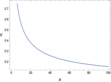
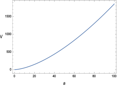
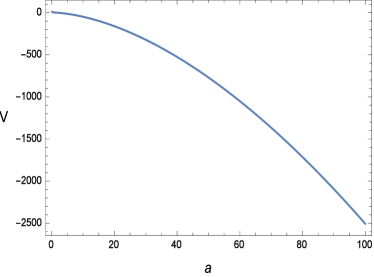
Figure 1: Plot of field Potential versus scale factor “a” with $\alpha_{1}=-2\times 10^{-10}$, $\alpha_{2}=-10^{-10}$, $\alpha_{3}=3\times 10^{8}$, $n=0.05$, $\beta=5\times 10^{-5}$, $\omega_{0}=-5\times 10^{-24}$ and $H_{0}=67.3$ given by Eq. (III.1).

Figure 2: Plots of field Potential versus scale factor “a” with $\alpha_{1}=-0.2$, $\alpha_{2}=1$, $n=1.5$, $\beta=0.5$ and $\omega_{0}=-2$ given in Eqs. (IV.1.3) and (IV.2.3).

Appendix A

Eq. (II) in terms of $``a"$ can be written as

$$6a^{2}H^{3}\phi^{\prime\prime}f_{R\phi}+12a^{2}H^{3}\left(3H^{2}+2aHH^{\prime}\right)\phi^{\prime\prime}f_{Y\phi}+\left(24aH^{3}+18a^{2}H^{2}H^{\prime}\right)\phi^{\prime}f_{R\phi}+\left(2a^{4}H^{4}H^{\prime\prime\prime}+38\right.$$

$$\left.\times a^{3}H^{4}H^{\prime\prime}+8a^{4}H^{3}H^{\prime}H^{\prime\prime}+214a^{2}H^{4}H^{\prime}+88a^{3}H^{3}{H^{\prime}}^{2}+2a^{4}H^{2}{H^{\prime}}^{3}+32aH^{5}\right)\phi^{\prime}f_{Y\phi}-36aH^{2}\times$$

$$\left(a^{2}H^{2}H^{\prime\prime}+a^{2}H{H^{\prime}}^{2}+5aH^{2}H^{\prime}\right)\phi^{\prime}f_{RR\phi}+36aH^{2}\left(2a^{2}H^{4}H^{\prime\prime}+2a^{3}H^{3}H^{\prime}H^{\prime\prime}+2aH^{4}H^{\prime}+4a^{2}H^{3}\right.$$

$$\left.\times{H^{\prime}}^{2}+2a^{3}H^{2}{H^{\prime}}^{3}\right)\phi^{\prime}f_{RY\phi}+72aH^{2}\left(24a^{2}H^{6}H^{\prime\prime}+34a^{3}H^{5}H^{\prime}H^{\prime\prime}+12a^{4}H^{4}{H^{\prime}}^{2}H^{\prime\prime}+96aH^{6}H^{\prime}\right.$$

$$\left.+154a^{2}H^{5}{H^{\prime}}^{2}+78a^{3}H^{4}{H^{\prime}}^{3}+12a^{4}H^{3}{H^{\prime}}^{4}\right)\phi^{\prime}f_{YY\phi}+6a^{2}H^{3}{\phi^{\prime}}^{2}f_{R\phi\phi}-6a^{2}H^{3}\omega(\phi){\phi^{\prime}}^{2}+12a^{2}H^{3}$$

$$\times\left(2aHH^{\prime}+3H^{2}\right){\phi^{\prime}}^{2}f_{Y\phi\phi}+6\left(7aH^{2}H^{\prime}+a^{2}H{H^{\prime}}^{2}+a^{2}H^{2}H^{\prime\prime}\right)f_{R}+2\left(a^{4}H^{4}H^{\prime\prime\prime\prime}+10a^{3}H^{4}H^{\prime\prime\prime}\right.$$

$$\left.+7a^{4}H^{3}H^{\prime}H^{\prime\prime\prime}+25a^{2}H^{4}H^{\prime\prime}+49a^{3}H^{3}H^{\prime}H^{\prime\prime}+11a^{4}H^{2}{H^{\prime}}^{2}H^{\prime\prime}+4a^{4}H^{3}{H^{\prime\prime}}^{2}+3aH^{4}H^{\prime}+49a^{2}\times\right.$$

$$\left.H^{3}{H^{\prime}}^{2}+19a^{3}H^{2}{H^{\prime}}^{3}+a^{4}H{H^{\prime}}^{4}\right)f_{Y}-36\left(a^{3}H^{4}H^{\prime\prime\prime}+7a^{2}H^{4}H^{\prime\prime}+5a^{3}H^{3}H^{\prime}H^{\prime\prime}+5aH^{4}H^{\prime}+17\right.$$

$$\left.\times a^{2}H^{3}{H^{\prime}}^{2}+2a^{3}H^{2}{H^{\prime}}^{3}\right)f_{RR}+36\left(2a^{3}H^{6}H^{\prime\prime\prime}+2a^{4}H^{5}H^{\prime}H^{\prime\prime\prime}+6a^{2}H^{6}H^{\prime\prime}+24a^{3}H^{5}H^{\prime}H^{\prime\prime}+2a^{4}\right.$$

$$\left.\times H^{5}{H^{\prime\prime}}^{2}+14a^{4}H^{4}{H^{\prime}}^{2}H^{\prime\prime}+2aH^{6}H^{\prime}+18a^{2}H^{5}{H^{\prime}}^{2}+22a^{3}H^{4}{H^{\prime}}^{3}+6a^{4}H^{3}{H^{\prime}}^{4}\right)f_{RY}+72\left(24a^{3}\right.$$

$$\left.\times H^{8}H^{\prime\prime\prime}+34a^{4}H^{7}H^{\prime}H^{\prime\prime\prime}+12a^{5}H^{6}{H^{\prime}}^{2}H^{\prime\prime\prime}+144a^{2}H^{8}H^{\prime\prime}+34a^{4}H^{7}{H^{\prime\prime}}^{2}+486a^{4}H^{6}{H^{\prime}}^{2}H^{\prime\prime}+578\right.$$

$$\left.\times a^{3}H^{7}H^{\prime}H^{\prime\prime}+24a^{5}H^{6}H^{\prime}{H^{\prime\prime}}^{2}+108a^{5}H^{5}{H^{\prime}}^{3}H^{\prime\prime}+438a^{4}H^{5}{H^{\prime}}^{4}+48a^{5}H^{4}{H^{\prime}}^{5}+1158a^{3}H^{6}{H^{\prime}}^{3}\right.$$

$$\left.+980a^{2}H^{7}{H^{\prime}}^{2}+96aH^{8}H^{\prime}\right)f_{YY}=0$$ (A.1)

V Conclusions

In this paper, we have examined the scalar field potentials by a procedure known as reconstruction of field potentials. We have used flat FRW model in a well-known general scalar tensor gravity. We have derived the general form of field potential without using any specific value of $f$, $V$ and $H$. In this paper, we have investigated the field potentials by taking three de-Sitter and two power law models which were constructed in 54a . We have taken $\omega=\omega_{0}\phi^{m}$ in all cases and field potential is based on scale factor $``a"$, scalar field $\phi$ and Hubble parameter $H$. It is noticed that without choosing any specific value of Hubble parameter, it is impossible to obtain the explicit form of field potential. For this reason, we consider the Hubble parameter for barotropic fluid, the cosmological constant and the Chaplygin gas matter contents in separate cases. In literature, the scalar field potentials which usually studied are positive and inverse power laws, exponential and logarithmic potentials 62 ; 63 , whereas others are different combinations of these functions.

In de-Sitter models, we have found the form of potential by reconstruction in terms of scalar field. We have found the scale factor in terms of scalar field with negative power in all cases of de-Sitter and in case of power law models, we cannot get the explicit potential but using barotropic fluid, cosmological constant and Chaplygin gas matter content with $\omega(\phi)=\omega_{0}\phi^{m}$, we have found the explicit form of scalar field potential.

Graphically we have showed here just three plots, de-Sitter $f(R,Y,\phi)$ model, power law $f(R,\phi)$ and $f(Y,\phi)$ models for Chaplygin gas matter content. In de-Sitter $f(R,Y,\phi)$ model the two cases $\alpha_{1}>0,~{}\alpha_{2}>0$ and $\alpha_{1}>0,~{}\alpha_{2}<0$ we have positive decreasing scalar field if $\alpha_{3}$ and $\omega_{0}>0$ have same sign and positive increasing scalar field if $\alpha_{3}$ and $\omega_{0}>0$ have opposite sign. In other two cases: $\alpha_{1}<0,~{}\alpha_{2}>0$ and $\alpha_{1}<0,~{}\alpha_{2}<0$, we have positive increasing scalar field if $\alpha_{3}$ and $\omega_{0}>0$ have same sign and positive decreasing scalar field if $\alpha_{3}$ and $\omega_{0}>0$ have opposite sign.

Observing power law models, we have noticed that we have four cases: $\alpha_{1}$ $\alpha_{2}$ both as positive, having opposite signs and both are negative. In $f(R,\phi)$ model, we have positive increasing scalar field potential for all cases if $\omega_{0}<0$ and negative decreasing scalar field potential if $\omega_{0}>0$. In $f(Y,\phi)$ model, two cases having $\alpha_{2}>0$ we have negative decreasing field potential for $\omega_{0}<0$ and for $\omega>0$ plot has signature flip from negative to positive if $\alpha_{1}>0$ and signature flip from positive to negative if $\alpha_{1}<0$. Other two cases having $\alpha_{2}<0$, for $\omega_{0}>0$ we have positive increasing field potential and signature flip from positive to negative if $\alpha_{1}<0$ and for $\alpha_{1}>0$ signature flip from negative to positive.

In 30 author has used the scalar-tensor gravity with flat FLRW and used induced gravity to reconstruct the scalar field potential. Further used barotropic fluid, cosmological constant, Chaplygin gas and modified Chaplygin gas to reconstruct the Scalar field potential. In same theory, Sharif and Saira 53 has used Bianchi-I universe model and induced gravity to reconstruct the scalar field potential. Further they also used barotropic fluid, cosmological constant and Chaplygin gas to reconstruct the Scalar field potential. Now in this paper, we are working on more extended scalar tensor theory with FLRW universe, used some de-Sitter and power law models to reconstruct the scalar field potential, de-Sitter models are not used before to reconstruct the scalar field potential. We also used barotropic fluid, cosmological constant and Chaplygin gas to reconstruct the Scalar field potential. In Lagrangian, if we choose $f(R,Y,\phi)=Rf(\phi)$,$\omega(\phi)=-1/2$, we get same Friedman equations, Klein-Gordon equation and scalar field potential constructed in 30 . If in power law $f(R,\phi)$ model, we choose parameters $\alpha_{1}=1/2$, $\alpha_{2}=\gamma$, $\gamma_{1}=2$, $\gamma_{2}=1$,$\gamma_{3}=\gamma_{4}=\gamma_{5}=\gamma_{6}=0$, we get the same formula of induced gravity and from this, we can get the same results.

References

- (1) Riess, A. et al.: Astron. J. 116 (1998) 1009; Perlmutter, S. J. et al.: Astro phys. J. 517 (1999) 565.
- (2) Padmanabhan, T.: Phys. Rep. 380 (2003) 235; Frampton, P. arXiv:astro-ph/0409166; Copeland, E. J., Sami, M. and Tsujikawa, Sh.: Int. J. Mod. Phys. D 15 (2006) 1753; Dolgov, A. D.: Phys. Part. Nucl. 43 (2012) 273; Bamba, K., et al.: Astro phys. Space Sci. 342 (2012) 155 ; Sahni, V. and Starobinsky, A. A.: Int. J. Mod. Phys. D 09 (2000) 373; Peebles, P. J. E. and Ratra, B.: Rev. Mod. Phys. 75 (2003) 559; Sahni, V.: Classical Quantum Gravity 19 (2002) 3435; Sahni, V. and Starobinsky, A. A.: Int. J. Mod. Phys. D 15 (2006) 2105.
- (3) Fujii, Y. and Maeda, K.: The Scalar-Tensor Theory of Gravitation (Cambridge University Press, Cambridge, England, 2004).
- (4) Nojiri, S. and Odintsov, S. D.: Int. J. Geom. Methods Mod. Phys. 4 (2007) 115; Nojiri, S. and Odintsov, S. D.: Phys. Rep. 505 (2011) 59.
- (5) Capozziello, S. and Faraoni, V., Beyond Einstein Gravity: A Survey of Gravitational Theories for Cosmology and Astrophysics, Fundamental Theories of Physics Vol. 170 (Springer, New York, 2011).
- (6) Capozziello, S. and Laurentis, M. D.: Phys. Rep. 509 (2011) 167.
- (7) Felice, A. D. and Tsujikawa, S.: Living Rev. Relativity 13 (2010) 3.
- (8) Starobinsky, A. A.: Lect. Notes Phys. 246 (1986) 107; Linde, A. D.: Particle Physics and Inflationary Cosmology (Harwood, Chur, Switzerland, 1990).
- (9) Lidsey, J. E. et al.: Rev. Mod. Phys. 69 (1997) 373; Peterson, C. M. and Tegmark, M.: Phys. Rev. D 83 (2011) 023522; Pi, S. and Sasaki, M.: J. Cosmol. Astropart. Phys. 10 (2012) 051.
- (10) Elizalde, E. et al.: Phys. Rev. D 77 (2008) 106005.
- (11) Starobinsky, A. A.: JETP Lett. 68 (1998) 757.
- (12) Burd, A. B. and Barrow, J. D.: Nucl. Phys. B 308 (1988) 929.
- (13) Barrow, J. D.: Phys. Lett. B 235 (1990) 40.
- (14) Yurov, A.: Eur. Phys. J. Plus 126 (2011) 132.
- (15) Guo, Z. K., Ohta, N. and Zhang, Y. Z.: Mod. Phys. Lett. A 22 (2007) 883.
- (16) Guo, Z. K., Ohta, N. and Zhang, Y. Z.: Phys. Rev. D 72 (2005)023504.
- (17) Saini, T. D. et al.: Phys. Rev. Lett. 85 (2000) 1162.
- (18) Aref’eva, I. Y., Koshelev, A. S. and Vernov, S. Y.: Theor. Math. Phys. 148 (2006) 895.
- (19) Capozziello, S., Nojiri, S. and Odintsov, S. D.: Phys. Lett. B 634 (2006) 93.
- (20) Muslimov, A. G.: Classical Quantum Gravity 7 (1990) 231; Salopek, D. S. and Bond, J. R.: Phys. Rev. D 42 (1990) 3936; Zhuravlev, V. M., Chervon, S. V. and Shchigolev, V. K.: J. Exp. Theor. Phys. 87 (1998) 223; Bazeia, D. et al.: Phys. Lett. B 633 (2006) 415; Townsend, P. K.: Classical Quantum Gravity 25 (2008) 045017; Yurov, A. V.: Theor. Math. Phys. 166 (2011) 259; Kamenshchik A. Y. and Manti, S.: Gen. Relativ. Gravit. 44 (2012) 2205; Kim, H. C.: Mod. Phys. Lett. A, 28 (2013) 1350089.
- (21) Nojiri, S. and Odintsov, S. D.: J. Phys. Conf. Ser. 66 (2007) 012005.
- (22) Aref’eva, I. Y., Koshelev, A. S. and Vernov, S. Y.: Phys. Rev. D 72 (2005) 064017; Vernov, S. Y.: Theor. Math. Phys. 155 (2008) 544.
- (23) Andrianov, A. A. et al.: J. Cosmol. Astropart. Phys. 02 (2008) 015.
- (24) Aref’eva, I. Y., Bulatov, N. V. and Vernov, S. Y. Theor. Math. Phys. 163 (2010) 788.
- (25) Padmanabhan, T.: Phys. Rev. D 66 (2002) 021301.
- (26) Feinstein, A.: Phys. Rev. D 66 (2002) 063511.
- (27) Gorini, V. et al.: Phys. Rev. D 69 (2004) 123512.
- (28) Shchigolev, V. K. and Rotova, M. P.: Mod. Phys. Lett. A 27 (2012) 1250086.
- (29) Boisseau, B. et al.: Phys. Rev. Lett. 85 (2000) 2236.
- (30) Kamenshchik, A. Y., Tronconi, A. and Venturi, G.: Phys. Lett. B 702 (2011) 191.
- (31) Qiu, T.: J. Cosmol. Astropart. Phys. 06 (2012) 041; Phys. Lett. B 718 (2012) 475.
- (32) Bamba, K., Nojiri, S. and Odintsov, S. D.: Phys. Rev. D 77 (2008) 123532; Elizalde E. and Lpez-Revelles, A. J.: Phys. Rev. D 82 (2010) 063504; Elizalde, E. et al.: Phys. Atom. Nucl. 76 (2013) 996.
- (33) Cruz-Dombriz, A. D. L. and Dobado, A.: Phys. Rev. D 74 (2006) 087501; Cruz-Dombriz A. D. L. and SaezGomez, D.: Classical Quantum Gravity 29 (2012) 245014.
- (34) Nojiri, S. and Odintsov, S. D.: Phys. Rev. D 74 (2006) 086005; Dunsby, P. K. S. et al.: Phys. Rev. D 82 (2010) 023519; Myrzakulov, R., Gomez, D. S. and Tureanu, A.: Gen. Relativ. Gravit. 43 (2011) 1671.
- (35) Jamil, M. et al.: Eur. Phys. J. C 72 (2012) 1999; Bamba, K. et al.: Phys. Rev. D 85 (2012) 104036.
- (36) Deffayet C. and Woodard, R. P.: J. Cosmol. Astropart. Phys. 08 (2009) 023.
- (37) Koivisto, T. S.: Phys. Rev. D 77 (2008) 123513; Elizalde, E., Pozdeeva, E. O. and Vernov, S. Y.: Phys. Rev. D 85 (2012) 044002; Vernov, S. Y.: Phys. Part. Nucl. 43 (2012) 694; Elizalde, E., Pozdeeva, E. O. and Vernov, S. Y.: Classical Quantum Gravity 30 (2013) 035002.
- (38) Lidsey, J.E. et al.: Rev. Mod. Phys. 69 (1997) 373; Copeland, E.J., Sami, M. and Tsujikawa, S.: Int. J. Mod. Phys. D 15 (2006) 1753; Frieman, J.A., Turner, M.S. and Huterer, G.: Ann. Rev. Astron. Astrophys. 46 (2008) 385.
- (39) Capozziello, S., Nojiri, S. and Odintsov, S. D.: Phys. Lett. B 634 (2006) 93; Kamenshchik, A. Y. and Manti, S.: Gen. Relativ. Gravit. 44 (2012) 2205.
- (40) Cooper F. and Venturi, G.: Phys. Rev. D 24 (1981) 3338.
- (41) Finelli, F., Tronconi, A. and Venturi, G.: Phys. Lett. B 659 (2008) 466.
- (42) Cerioni, A. et al.: Phys. Lett. B 681 (2009) 383.
- (43) Cerioni, A. et al.: Phys. Rev. D 81 (2010) 123505.
- (44) Tronconi, A. and Venturi, G.: Phys. Rev. D 84 (2011) 063517.
- (45) Kamenshchik, A. Y., Tronconi, A. and Venturi, G.: Phys. Lett. B 713 (2012) 358.
- (46) Sami, M. et al.: Phys. Rev. D 86 (2012) 103532.
- (47) Cota, J. L. C., Putter, R. D. and Linder, E. V.: J. Cosmol. Astropart. Phys. 12 (2010) 019.
- (48) Spokoiny, B. L.: Phys. Lett. B 147 (1984) 39; Futamase T. and Maeda, K. I.: Phys. Rev. D 39 (1989) 399; Salopek, D. S., Bond, J. R. and Bardeen, J. M.: Phys. Rev. D 40 (1989) 1753; Fakir R. and Unruh, W. G.: Phys. Rev. D 41 (1990) 1783.
- (49) Barvinsky, A. O. and Kamenshchik, A. Y.: Phys. Lett. B 332 (1994) 270; Nucl. Phys. B 532 (1998) 339; Barvinsky, A. O. et al.: Phys. Rev. D 81 (2010) 043530.
- (50) Kamenshchik, A. Y., Moschella, U. and Pasquier, V.: Phys. Lett. B 511 (2001) 265.
- (51) Kamenshchik, A. Y., Tronconi, A., Venturi, G. and Vernov, S.Y.: Phys. Rev. D 87 (2013) 063503.
- (52) Sharif, M. and Waheed, S.: Phys. Lett. B 726 (2013) 1.
- (53) Lambiase, G. et al.: JCAP. 07 (2015) 003.
- (54) Zubair, M. and Kousar, F.: EPJC. 76 (2016) 254.
- (55) Zubair, M. and Kousar, F.: Physics of the Dark Universe 14(2016)116-125.
- (56) Banerjee, N. and Pavon, D.: Phys. Lett. B 647 (2007) 477; Bertolami, O. and Martins, P. J.: Phys Rev D 61 (2000) 064007.
- (57) Sharif, M and Zubair, M.: J. Phys. Soc. Jpn. 82 (2013) 014002.
- (58) Sharif, M. and Zubair, M.: Gen. Relativ. Gravit. 46 (2014) 1723.
- (59) Bilic, N., Tupper, G. B. and Viollier, R. D.: Phys. Lett. B 535 (2002) 17.
- (60) Gorini, V., Kamenshchik, A. and Moschella, U.: Phys. Rev. D 67 (2003) 063509.
- (61) Sharif, M. and Waheed, S.: Int. J. Mod. Phys. D. 21 (2012) 1250055; J. Phys. Soc. Jpn. 81 (2012) 114901; J. Exp. Theor. Phys. 115 (2012) 599.
- (62) Demianski, M. et al.: Astronomy and Astrophys. 481 (2008) 279; Andrianov, A. A., Cannata, F. and Kamenshchik, A. Y.: J. Cosmol. Astropart. Phys. 10 (2011) 004; Rasouli, S. M. M., Farhoudi, M. and Sepangi, H. R.: Class. Quantum Grav. 28 (2011) 155004.