Tagging $b$ quarks without tracks using an Artificial Neural Network algorithm

Abstract

Pixel detectors currently in use by high energy physics experiments such as ATLAS and CMS, are critical systems for tagging $B$ hadrons within particle jets. However, the performance of standard tagging algorithms begins to fall in the case of highly boosted $B$ hadrons ($\gamma\beta=p/m>200$). This paper builds on the work of our previous study that uses the jump in hit multiplicity among the pixel layers when a $B$ hadron decays within the detector volume. First, multiple $pp$ interactions within a finite luminous region were found to have little effect. Second, the study has been extended to use the multivariate techniques of an artificial neural network (ANN). After training, the ANN shows significant improvements to the ability to reject light-quark and charm jets; thus increasing the expected power of the technique.

• 15 June 2017

1 Introduction

Many of the most exciting searches for new physics beyond the Standard Model, as well as further studies of the Standard Model itself, benefit from being able to identify high-energy jets containing $b$ quarks (“$b$ jets”). Examples include Higgs pair production and decay via $HH\rightarrow b\overline{b}b\overline{b}$, sensitive to Higgs trilinear couplings [1, 2]; graviton and radion decays to heavy fermions and bosons in warped extra dimension models [3]; third-generation superpartners in supersymmetry [4]; and indeed any new physics with preferential couplings to heavy Standard Model particles or third-generation fermions in particular.

Because $B$ hadron tagging is so important, progress has been made by the CMS and ATLAS experiments in improving the effiency of their conventional taggers. They have been mainly using boosted decision tree techniques and also some artificial neural nets to make gains in discriminating power at higher jet energies. The interested reader can find this information in references [5], [6], [7] (and references contained within these reports). In particular we see in figure 25(a) in [5] that the CMS collaboration has managed to obtain$~{}\sim 20\%$ efficiency at jet $p_{T}\simeq 800$ GeV while figure 5 within [6] shows better than $60\%$ efficiency but only to jet $p_{T}\simeq 400$ GeV. Even with these improved results it is still clear that maintaining high $b$-tagging efficiency out to TeV-scale jet $p_{T}$ is a difficult problem.

This work follows from a previous study by two of the current authors [8]. Section 2 will summarise that previous study. Section 3 will explain the simulations used, the modifications, and the improvements to those simulations implemented by the authors. Section 4 will introduce and explain the implementation of an Artifical Neural Network (ANN) in order to investigate the level of improvement to $b$-tagging efficiency and light quark rejection in multi-TeV jets. We will show the results of these new studies in section 4.2 while section 6 concludes.

2 The “multiplicity jump” tagger

The principle underlying our previous study (see[8] and references therein) is the fact that in hadron colliders, a $B$ hadron with $\gamma\beta>200$ and typical proper lifetime in the $\approx 1$ ps range, will have a significant probability of passing through the inner layers of the detectors that surround the interaction point (see Figure 1). Since the assumption underlying many tracking algorithms is that any fiducial track ought to leave a signal all the way to the inner layers, there is a significant chance that the tracks found would be missing hits on the inner layers, or might even have hits assigned incorrectly.

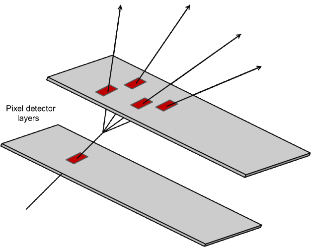
Figure 1: The “multiplicity jump” tagger works when a particle with a large Lorentz boost decays between two pixel layers. Shown here schematically is a particle traversing a pixel layer from the lower left and decaying before the next layer, causing multiple hits to appear. If highly boosted, $B$ hadrons have this property.

A basic Geant4 detector simulation was used consisting of four cylindrical layers of silicon which were segmented to approximate a typical pixel detector as realized in LHC experiments such as ATLAS or CMS. Pythia8+EvtGen were used to simulate the physics process where TeV mass $Z^{\prime}$ particles were created in order to produce high energy jets with $b$, $c$, and light quark progenitors. FastJet was used to identify the jet axis using the anti-$k_{T}$ algorithm with a cone $R=0.2$.

A “hit” in the detector was defined as a pixel segment in which at least 0.05 MeV had been deposited. Hits within a narrow cone around the jet axis of $\Delta R\equiv\sqrt{\Delta\eta^{2}+\Delta\phi^{2}}<0.04$ were used to define the relative multiplicity jump $f_{j}$ between layers $j$ and $j+1$,

$$f_{j}=\frac{N_{j+1}-N_{j}}{N_{j}}=\frac{\Delta N_{j}}{N_{j}},$$ (1)

where $N_{j}$ is the number of hits in pixel layer $j$. A jet was tagged as a $b$ jet if $f_{j}$ equaled or exceeded a value $1$ for any layer $j$. The resulting tagging efficiency as a function of the parent jet energy showed clear separation between the tagging of $b$ over light-quark jets, and that the $b$-tagging efficiency remained fairly stable up to roughly 1.5 TeV. This promising result, however, was obtained in simulations without additional pile-up interactions or a finite luminous region along the beam line. It was also suggested that it would be worthwhile to investigate if machine learning techniques could further optimise the combination of the new $f_{j}$ observables. This paper addresses these points.

3 Simulation

The authors continued to use a simulation based on Geant4 (version 10.0) to model particle interactions and showering in a detector[9][10]. Pythia version 8.209[11], with the default Monash 2013 tune[12], was used to simulate $pp$ collisions with center-of-mass energy $\sqrt{s}=13\;{\rm TeV}$. Hard QCD events were generated with a Poisson mean of 45 soft QCD (minimum bias) pile-up interactions for each hard QCD collision. The hard QCD process was set to have a minimum $P_{T}>700$ GeV for the underlying tree-level interactions, and reconstructed jets with $P_{T}>350$ GeV from FastJet were used.

Hard QCD from Pythia was also used to create a pure sample of 300,000 $b$ jets (also with pile-up) that were used to enrich the $B$ hadron content of the sample. Simulations indicate the $B$ hadron takes most of the jet energy, with the most likely energy fraction being $\simeq 85\%$, independent of the primary $b$ parton energy[13]. Decays of $B$ hadrons were simulated using EvtGen version 1.4.0, with bremsstrahlung handled by Photos version 3.52 and any $\tau$ decays by Tauola version 1.0.7[14]. All of the events (hard QCD and pile-up) had collisions distributed along the beam-line with a Gaussian probability distribution having a width of $45$ mm.

A simplified detector geometry, loosely based on the four-layer ATLAS pixel barrel system, was used to model the detector response. The active pixel layers, with radii 25.7, 50.5, 88.5, and 122.5 mm, were encased within a volume of air and inside a uniform 2 T magnetic field pointing in the positive $z$ direction. Each barrel was 1.3 m long (the innermost layer, the “Insertable $B$ Layer” or IBL, of the ATLAS pixel system is actually slightly shorter[15]). The pixel sensors were $300\;{\rm\mu m}$ thick, with a $50\;{\rm\mu m}$ pitch in the $\phi$ direction, and a $400\;{\rm\mu m}$ length in the $z$ direction ($250\;{\rm\mu m}$ in our innermost layer, similar to the IBL in ATLAS). These idealized pixels were simulated as pure silicon slabs without gaps.

In order to model inactive material, further cylinders of silicon were added to the Geant4 model, located just outside each cylinder of sensitive pixels, so as to bring the total simulated material up to an equivalent of 2.5% of radiation length per layer. In addition a silicon cylinder half as thick was added just inside the outermost active layer of pixels.

Stable generated particles (excluding neutrinos) were clustered using the FastJet (version 3.1.3)[16] implementation of the “anti-$k_{T}$” sequential recombination algorithm[17] with $R=0.2$. The jet’s axis was corrected for the position of the primary vertex and was then used to define the angular search region in the multiplicity jump algorithm.

The sample of $b$ jets was defined by finding the highest energy ground state $B$ hadron within $\Delta R<0.2$ of the jet axis. After $b$ jets were identified, a similar search was performed to identify charm jets. All other jets were considered “light quark” jets (or “uds”) jets. The two highest energy $b$ jets were then used to test the efficiency of the multiplicity jump algorithm.

4 Performance

4.1 Effect of pile-up

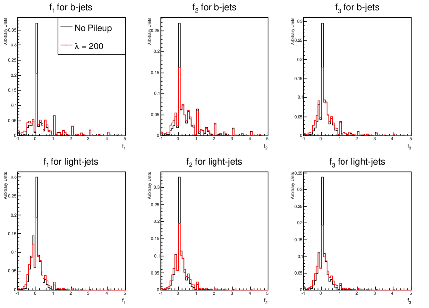
Figure 2: Shown are the histograms of the quantity $f_{j}$ for each of the three gaps within the simulated pixel detector comparing the case with no pile-up (black) and with an average of $\lambda=200$ pile-up events (red). The probability of obtaining a negative or zero value for $f_{j}$ has increased; however the key feature, that $b$ jets have a substantial positive tail compared to uds-jets, remains.

Figure 2 shows histograms of $f_{j}$ from equation 1 for $b$ and light-quark jets for no pile-up and events with an average of $\lambda=200$ (rather than the nominal 45) additional interactions spread over the luminous region. It is clear that, having corrected the jet axis for the primary vertex position, the narrow search cone, $\Delta R<0.04$, excludes most additional pile-up hits. The histograms indicate that the main effect of pile-up is to reduce the chance that $f_{j}=0$, which only occurs when the number of hits between the layers in question within the search cone are the same. Comparing the $b$ jet and uds-jet cases one can see that, regardless of pile-up, the $b$ jets still have long tails for $f_{j}\geq 1.0$. Since this region of $f_{j}$ is largely insensitive to pile-up, we conclude that its effects on cut and neural net-based approaches to multiplicity jump tagging are similarly insensitive. Nevertheless, we continued to simulate an average of 45 pile-up interactios per event for other studies in this article.

4.2 Artificial Neural Network

Both CMS and ATLAS have already shown the benefits of using multivariate techniques such as boosted decision trees and artificial neural networks (ANN’s) for $b$-tagging at the LHC[18]. It is a natural next step to see what improvements might be possible within the multiplicity jump technique.

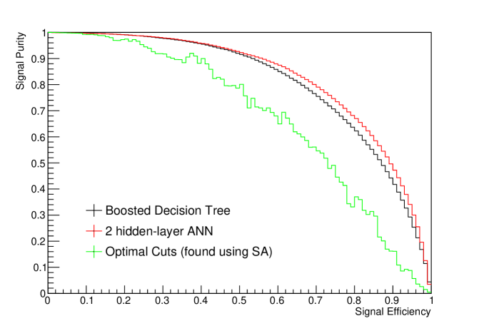
Figure 3: A comparison of the efficiency vs. purity of the ANN, a boosted decision tree, and the simple cut-based technique from reference[8].

The Toolkit for Multivariate Analysis (TMVA) packaged within ROOT (version 5.34.21)[19] was used to evaluate a set of multivariate analysis techniques in parallel, giving one information about the efficiency at various purity levels, and the integral of the efficiency-purity (the “ROC”) curve. Figure 3 shows a comparison of ROC curves for a Boosted Decision Tree (BDT), an ANN with two hidden layers (described below), and a cut-based analysis. Simulated annealing (SA) is used to determine the optimal set of cut values for a given efficiency. The ANN approach is preferred in this evaluation.

In figure 3, the BDT depth was 200 nodes. So the usual advantages (such as the ability to deduce its inner workings) typically conferred by decision trees over neural networks did not apply. Moreover, while a BDT is often faster to execute once trained, an ANN with only two internal layers is shallow enough that the difference in execution time is reduced, and could be further reduced using standard parallelism techniques.

The main ANN chosen has a single input layer with $N$ neurons, where $N$ is the number of input variables. There follow two hidden layers, the first with $N+5$ neurons and the second with 5 neurons. This second layer is connected to a single output neuron whose output spans the interval [0,1] and is used as the discriminant. The activation function used in the hidden layers is $f(x)=\tanh{(x)}$, where $x$ is the weighted sum of the outputs of the previous layer. Tests using up to eight hidden layers responded with identical results on identical samples as two layers. At the same time, two layers were chosen in order to satisfy the requirements of the universal approximation theorem[20].

The list of inputs is as follows:

• jet $P_{T}$, energy, and mass from the anti-$k_{T}$ jet;
  

• The raw hit numbers in each layer within the search cone of $R<0.04$ of the jet axis;
  

• each of the $f_{i}$ as defined in equation 1; and
  

• the maximum of the $f_{i}$ (max($f_{i}$)) over all the layers.
  

Note the input variables overlap somewhat: in principle an ANN should be able to use the $f_{i}$ automatically to obtain the equivalent discrimination power that max($f_{i}$) provides. However, prior knowledge applied to the inputs to an ANN will improve the efficiency of the training phase: using max($f_{i}$) as an input saves the ANN from having to derive an equivalent. At the same time, should max($f_{i}$) prove of little use, the ANN should de-weight that input in favour of more powerful combinations.

The neural network is trained using standard back-propagation techniques on a dataset of 1 million hard QCD events (including $b$ jets) and enriched with 300,000 hard QCD events that resulted in $B$ hadron production. For training, a “signal” event was a $b$ jet with a $B$ hadron that decayed within the fiducial volume. A “background” event was anything that was not a $b$ jet.

The test sample consisted of 1 million hard QCD events with an average of 45 pile-up events, generated in the same way but with a different random number seed. No additional $b$ jets were added. The resulting discriminant distribution is shown in figure 4. $b$ jets are strongly peaked towards a value of 1, while uds jets are strongly peaked towards low values. Charm jets which decay within the fiducial region, on the other hand, are distributed roughly evenly across the discriminant range, which is not surprising since the ANN was trained to recognize only $b$ jets as signal.

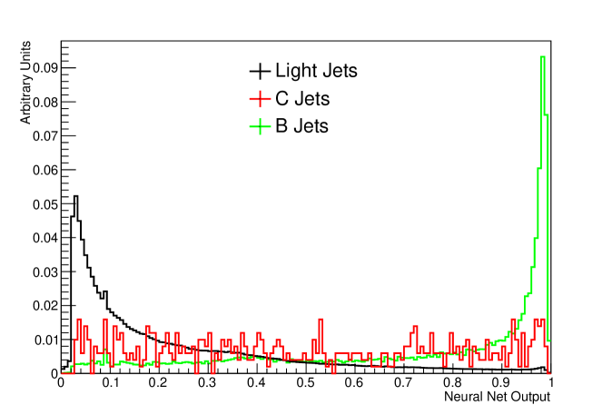
Figure 4: The distribution of the ANN output. $b$, $charm$, and $uds$ jets are identified by colour. The charm and bottom jets plotted here are only those jets where the final state hadron decayed within the fiducial volume.

4.3 ANN results

In order to measure the algorithm’s performance in our simulation, we define an efficiency $\epsilon_{b}$ for $b$ jets in a fiducial region as the number of tagged $b$ jets divided by the number of jets in which the matched $B$ hadron decays within the fiducial region. The fiducial region is defined in terms of the inner and outer pixel layers being investigated; in other words, the $\epsilon_{b}$ reflects the probability that, if a $B$ hadron decays between the inner and outer layers, it will be tagged by the algorithm. The light-quark “efficiency” $\epsilon_{q}$ is the number of light-quark jets tagged by the algorithm divided by the number of light-quark jets.

To see how the tagging efficiency behaves as a function of the jet energy for a given cut on the ANN output, we use a figure of merit designed to optimize the significance of the tagged B jets over the light quark jets. (Charm jets are explicitly excluded at this point.) The figure of merit used is

$$S=\frac{\epsilon_{b}}{\sqrt{\epsilon_{q}}}$$ (2)

where $\epsilon_{b}$ and $\epsilon_{q}$ are the efficiency of the tag on $b$ jets and the mistag rate for light quark jets, respectively. There are a few different ways of quantifying significance-like values. In this case $S$ has the advantage of being independent of the absolute numbers of the different types of jets and should be independent of specific underlying jet production mechanisms.

Figure 5 shows the $b$ jet efficiency and the mistag percentage of light-quark jets vs. jet energy for an ANN output value greater than $0.9$. The cut-based results on the same sample are also shown. Choosing an ANN output $>0.9$, where the significance defined in equation 2 is near the maximum, optimizes the statistical power of finding $b$ jets over light quark jets. With this optimization the loss in efficiency is compensated by the ability to discriminate against uds jets.

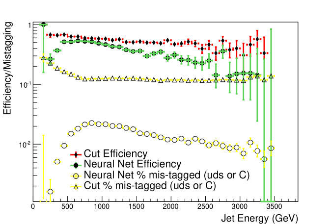
Figure 5: Efficiencies and mistag rates for the ANN and cut-based tagging algorithms. The ANN algorithm uses a value greater than $0.9$ from figure 4, while the cut-based algorithm tags jets with $\max(f_{j})\geq 1$.

When the highest significance is used, the absolute efficiency obtained from the ANN does not exceed what was achieved with a cut-based approach using a similar significance metric. So we also show a case with the ANN discriminate greater than 0.75, chosen to match the $b$ jet efficiencies of the ANN and cut-based algorithms. This is shown in figure 6 where the multivariate technique still outperforms the cut-based method in rejecting uds jets.

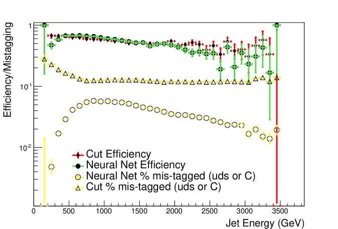
Figure 6: Efficiencies and mistag rates for the ANN and cut-based tagging algorithms as in figure 5. Here a value of the ANN output greater than 0.75 is set so as to match the cut-based b-tagging efficiency.

5 Cross checks and Further tests

Artificial neural networks are difficult to characterize and can lead to false training, where the quantity the user thinks is providing the discriminating power is actually being bypassed in favor of a nonsensical combination. One concern here is that, because the $B$ hadron fraction might be a function of the jet energy, the ANN could rely too heavily on this or other energy-related quantities. One of the reasons high mass $Z^{{}^{\prime}}$ states were chosen for both the signal and background jet samples is so that the energy spectrum of the resulting jets would be the same.

In order to test for this possibility, the training was repeated on a hard QCD jet sample with a flat energy distribution from 1 to 6 TeV. After re-training, however, the efficiency and mistag rates for a given cut on the discriminant were virtually the same and behaved similarly as a function of jet energy, suggesting that false training on jet energy, at least, was not a problem. Additionally tests we performed upon the trained ANN show that changes in the jet energy, jet mass, and jet $P_{T}$ have at least an order of magnitude smaller impact on the ANN output compared to inputs like $f_{i}$ or max($f_{i}$) which are related to hits. (See subsection 5.1 below.)

The effect of the inactive material mentioned in section 3 on mistag rates was investigated by removing the inactive material and generating a new test sample. The ANN was not re-trained. The mistag rates for both cut-based and ANN-based analyses fall, but that for the ANN falls much more. The overall $b$-tagging efficiency also drops somewhat, possibly due to the fact that the ANN was trained on a sample simulated with the extra material.

The ANN-based tagger, like the cut-based tagger, exhibits a fall in efficiency at jet energies above 1 TeV. Since the efficiency as defined above counts only those $B$ hadrons which could in principle have been detected by a multiplicity jump, any loss of $B$ hadrons because they live too long ought to have been removed. However, since some 85% of $B$ hadrons decay into charm hadrons with a similar lifetime, it is suspected that the ANN uses combinations of hits in different layers that would benefit from the charm decay; with highly boosted hadrons, it is more likely that the charm daughter would live long enough to escape the pixel volume. This hypothesis was tested by adding a fifth pixel layer at higher radius, and it was observed that the $b$-tagging efficiency was maintained for higher energy jets.

5.1 Input weights

To gain insight into which inputs were being most heavily weighted after training, we generated maps of the weights between the input and the ANN’s first hidden layer. This is shown in Figure 7, where the weight that the trained neural net assigns to an input has been indicated by a color, with a darker color indicating a high weight. By looking at Figure 7 we can see that all of the kinematic variables (like jet energy) have small weights. This indicates, in addition to the studies explained previously, that the jet-related inputs have small individual effects.

Figure 7 shows that the $JetHit1$ and $JetHit4$ variables were heavily weighted. Moreover they are anti-correlated, i.e. when $JetHit1$ is heavily positively weighted, $JetHit4$ is highly negatively weighted, and vice versa.

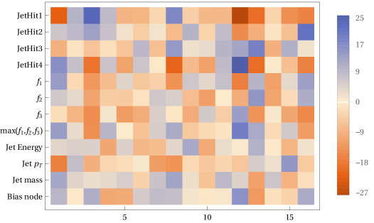
Figure 7: A “heatmap” of the weights $w_{ij}$ between the input and first hidden layers. The colors are an indication of how strongly positively or negatively the given input is influencing a given internal node of the ANN. Note the near complete anti-correlation between the number of hits in layer 1 (JetHit1) and layer 4 (JetHit4) for many internal nodes.

This analysis invites us to reason that some combination of $|JetHit4-JetHit1|$ is being used as a primary discriminant within the neural network. To investigate this, we show this hit difference for $b$ jets and uds jets in Figure 8. This showed that there was a significant separation in the distributions for $b$ and uds jets and so implied that it could be a powerful individual tagger.

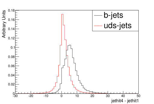
Figure 8: Plot showing $|JetHit4-JetHit1|$ for $b$ and uds jets. Based upon this plot and the heatmap of figure 7 it appears the ANN found a similar relationship to aid in tagging $b$ jets.

Finally, in order to fully satisfy ourselves that the jet kinematic variables were not having undue individual effect on the ANN, we calculated the analytic function for the ANN output in Mathematica. The partial derivatives of the ANN output with respect to the various inputs were computed. As expected, in general the derivatives for a given input are large where the heat map indicates a large effect on the output.

5.2 Changing the search cone

As mentioned in section 2 we used a fixed search cone for pixel hits of $\Delta R\leq 0.04$ in order to make comparisons to our previous work transparent[8]. But it is also clear from the previous studies that lower energy $b$ jets contain lower energy $B$ hadrons. In the Monte Carlo samples that we used $\Delta R\leq 0.04$ only contained about 85% of the $B$ hadrons. Indeed, the best solution would be to allow the ANN to choose hits within a variable cone size that would depend on the energy of the jet.

To do something very similar to an energy-dependent cone search new input discriminators, $JetHitN$ and $f_{N}$ (where $N$ is the layer number), were added to a new artificial neural net, each corresponding to cone sizes of $\Delta R\leq 0.04$, $\Delta R\leq 0.11$, and $\Delta R\leq 0.20$ thus increasing the number of inputs. Repeating the previous study for the number of internal layers indicated that a 4-layer ANN was needed to accomodate the increased complexity of inputs. This modified ANN was implemented and trained using a much larger training sample. Figure 9 shows the case where the 4-layer ANN output is chosen to match the light-quark rejection of the two-layer ANN case. One can see that improvements occur in the lower energy jets, consistent with the use of larger cone sizes. As the jet energy increases the benefits of having larger cones lessens such that there is no difference between the cases at the highest jet energies.

The training requirements for the multi-cone ANN were substantially more intensive than the previous 2-layer case. Training for the ANN that generated figure 5 required several hours while the training for the 4-layer case took 3 days on the same computer system. Training requirements could be a limitation for more complex neural nets.

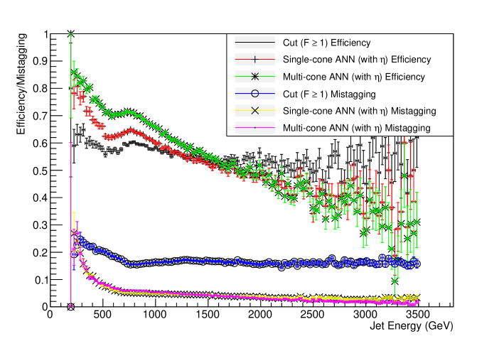
Figure 9: Shown is a comparison of the efficiency of the fixed-cone ANN from figure 5 and the ANN where mulitple inputs with search cones for hits of $R\leq 0.10$ and $R\leq 0.20$ were used in addition to the original search cone of $R\leq 0.04$. The 2 and 4-layer ANN outputs were chosen such that they matched in light quark rejection making a comparison of the $b$ jet tagging effectiveness more obvious.

6 Conclusions and further study

This article focuses on using an artificial neural network (ANN) to optimize the discriminating power that may be afforded by a jump in the numbers of hits from the inner to outer layers of a pixel detector in the presence of a highly boosted $B$ hadron.

This study accounts for pile-up at a similar level, and spread over a broad luminous region, as currently experienced by the LHC experiments. Additional studies using more internal node layers to accomodate a range of input variables that account for differing cone sizes showed improvements to $b$-tagging over a fixed cone size, but with the disadvantage of increased training requirements.

Other complications arising from realistic detector geometry, including overlaps between sensors comprising the same layer, and the transition from cylindrical to endcap disk layers, have still to be investigated. Nonetheless, the use of a multivariate technique has shown a significant improvement in the mistag rate for jets that did not contain a $B$ hadron. Training on charm jets with the addition of another output neuron may recover charm tags as well.

As noted in [8], if shown to work in the LHC detectors this technique could have implications for the detector design at future colliders such as the Future Circular Collider (FCC)[21]. Extending finely segmented pixel coverage to larger radii in order to tag these jets may be desirable for such future detectors.

References

References

- [1] F. Bishara, R. Contino and J. Rojo, Higgs pair production in vector-boson fusion at the LHC and beyond, 1611.03860.
- [2] J. K. Behr, D. Bortoletto, J. A. Frost, N. P. Hartland, C. Issever and J. Rojo, Boosting Higgs pair production in the final state with multivariate techniques, Eur. Phys. J. C76 (2016) 386, [1512.08928].
- [3] M. Gouzevitch, A. Oliveira, J. Rojo, R. Rosenfeld, G. P. Salam and V. Sanz, Scale-invariant resonance tagging in multijet events and new physics in Higgs pair production, JHEP 07 (2013) 148, [1303.6636].
- [4] J. Alwall, P. Schuster and N. Toro, Simplified Models for a First Characterization of New Physics at the LHC, Phys. Rev. D79 (2009) 075020, [0810.3921].
- [5] CMS collaboration, Identification of b quark jets at the CMS Experiment in the LHC Run 2, Tech. Rep. CMS PAS BTV-15-001, CERN, Geneva, May, 2016.
- [6] ATLAS collaboration, Identification of Jets Containing -Hadrons with Recurrent Neural Networks at the ATLAS experiment, Tech. Rep. ATL-PHYS-PUB-2017-003, CERN, Geneva, March, 2017.
- [7] ATLAS collaboration, Optimisation of the ATLAS -tagging performance for the 2016 LHC Run, Tech. Rep. ATL-PHYS-PUB-2016-012, CERN, Geneva, June, 2016.
- [8] B. T. Huffman, C. Jackson and J. Tseng, Tagging quarks at extreme energies without tracks, J. Phys. G43 (2016) 085001, [1604.05036].
- [9] GEANT4 collaboration, S. Agostinelli et al., GEANT4: A Simulation toolkit, Nucl. Instrum. Meth. A506 (2003) 250–303.
- [10] J. Allison et al., Geant4 developments and applications, IEEE Trans. Nucl. Sci. 53 (2006) 270.
- [11] T. Sjostrand, S. Mrenna and P. Z. Skands, A Brief Introduction to PYTHIA 8.1, Comput. Phys. Commun. 178 (2008) 852–867, [0710.3820].
- [12] P. Skands, S. Carrazza and J. Rojo, Tuning PYTHIA 8.1: the Monash 2013 Tune, Eur. Phys. J. C74 (2014) 3024, [1404.5630].
- [13] C. Peterson, D. Schlatter, I. Schmitt and P. M. Zerwas, Scaling Violations in Inclusive e+ e- Annihilation Spectra, Phys. Rev. D27 (1983) 105.
- [14] D. J. Lange, The EvtGen particle decay simulation package, Nucl. Instrum. Meth. A462 (2001) 152–155.
- [15] M. Capeans, G. Darbo, K. Einsweiller, M. Elsing, T. Flick, M. Garcia-Sciveres et al., ATLAS Insertable B-Layer Technical Design Report, Tech. Rep. CERN-LHCC-2010-013. ATLAS-TDR-19, CERN, Geneva, Sep, 2010.
- [16] M. Cacciari, G. P. Salam and G. Soyez, FastJet User Manual, Eur. Phys. J. C72 (2012) 1896, [1111.6097].
- [17] M. Cacciari, G. P. Salam and G. Soyez, The Anti-k(t) jet clustering algorithm, JHEP 04 (2008) 063, [0802.1189].
- [18] ATLAS collaboration, Optimisation of the ATLAS -tagging performance for the 2016 LHC Run, Tech. Rep. ATLAS-PHYS-PUB-2016-012, CERN, Geneva, June, 2016.
- [19] A. Hocker et al., TMVA - Toolkit for Multivariate Data Analysis, PoS ACAT (2007) 040, [physics/0703039].
- [20] K. Hornik, Approximation capabilities of multilayer feedforward networks, Neural Networks 4 (1991) 251–257.
- [21] TLEP Design Study Working Group collaboration, M. Bicer et al., First Look at the Physics Case of TLEP, JHEP 01 (2014) 164, [1308.6176].