Testing One Hypothesis Multiple Times

Sara Algeri^∗,† and David A. van Dyk^†

^∗University of Minnesota and ^† Imperial College London

Abstract: In applied settings, tests of hypothesis where a nuisance parameter is only identifiable under the alternative often reduces into one of Testing One Hypothesis Multiple times (TOHM). Specifically, a fine discretization of the space of the non-identifiable parameter is specified, and the null hypothesis is tested against a set of sub-alternative hypothesis, one for each point of the discretization. The resulting sub-test statistics are then combined to obtain a global p-value. In this paper, we discuss a computationally efficient inferential tool to perform TOHM under stringent significance requirements, such as those typically required in the physical sciences, (e.g., p-value $<10^{-7}$). The resulting procedure leads to a generalized approach to perform inference under non-standard conditions, including non-nested models comparisons.

Key words and phrases: Multiple hypothesis testing, bump hunting, non-identifiabily in hypothesis testing, non-nested models comparison.

1 Introduction

A fundamental statistical challenge in scientific discoveries is the so called “bump-hunting” problem (Choudalakis, 2011), where researchers aim to distinguish peaks due to a signal of interest (the new discovery) from peaks due to random fluctuations of the background. In the framework of hypothesis testing, the null model specified by $H_{0}$ is typically the background-only model, and a signal bump is added in the alternative model specified by $H_{1}$. Consider for example a dark matter search where we aim to distinguish events associated with a power-law (Pareto type I) distributed background from the signal of a dark matter source modeled as a narrow Gaussian bump with unknown location over the search area $\Theta\equiv[\mathcal{L},\mathcal{U}]\subset\mathbb{R}$. We can specify the model of interest using a mixture model

$$(1-\eta)\frac{1}{k_{\phi}y^{\phi+1}}+\frac{\eta}{k_{\theta}}\exp\biggl{\{}-\frac{(y-\theta)^{2}}{0.02\theta^{2}}\biggl{\}}\qquad\text{for $y\geq 1$,}$$ (1.1)

where $k_{\phi}$ and $k_{\theta}$ are normalizing constants, $y\geq 1$, $\phi>0$, and $\theta\geq 1$. Notice that the parameter $\theta$ characterizes both the location of the signal over the search region and its standard deviation. Specifically, the bump becomes wider the further its position is in the tail of the background distribution. The model in (1.1) is a toy example which simplifies the models involved in the context of searches for $\gamma$-ray emissions ina cluster of galaxies (Anderson et al., 2016); where for example the width of the signal may be a more complex function of its location. Despite its simplicity, the model in (1.1) introduces the key statistical issues arising in the context of dark matter searches, as described below.

In order to assess the evidence in favor of the signal, we test

$$H_{0}:\eta=0\quad\mbox{versus}\quad H_{1}:\eta>0.$$ (1.2)

where $\eta$ is the proportion of events due to the dark matter emission, and typically $0\leq\eta\leq 1$. Despite its straightforward formulation, testing (1.2) is non-trivial. Difficulties arise because $\theta$ is not defined under $H_{0}$. Consequently, classical asymptotic properties of, e.g., Maximum Lixelihood Estimates (MLE) and the Likelihood Ratio Test (LRT), fail. Analogously, complications may arise when using resampling techniques, such as bootstrapping (Efron and Tibshirani, 1994), to derive the null distribution of the test statistic, in the presence of stringent significance requirements. For searches in high energy physics for instance, the significance level necessary to claim a discovery can be in the order of $10^{-7}$ (see Lyons, 2013, Table 1). Hence, a large (e.g., $O(10^{8})$) simulation may be infeasible when dealing with complex models. This is a key motivation for a computationally efficient inferential solution.

To address these difficulties, in this paper, we consider the bump-hunting problem as a special case of what is known in statistical literature as “testing statistical hypotheses when a nuisance parameter is present only under the alternative”. In addition to bump-hunting, classical examples may include regression models where structural changes, such as break-points and threshold-effects, occur (Andrews, 1993; Hansen, 1992b, 1999; Davies, 2002).

The general problem has long been studied, starting at least from the seminal work of Hotelling (1939) and Davies (1977, 1987), and further investigated in the econometrics literature by several authors including Andrews and Ploberger (1994) and Hansen (1991, 1992a, 1996). In their practical implementation, these methods reduce the problem of testing with unidentifiable parameters under $H_{0}$ into one of Testing One Hypothesis Multiple times (TOHM), where a single null hypothesis $H_{0}$ is tested against different sub-alternative hypotheses of the form $H_{1}(\theta)$, one for each fixed $\theta$ in $\Theta$, and a corresponding ensemble of sub-test statistics indexed by $\theta$, namely $W(\theta)$, is specified. The goal is to provide a global p-value as the standard of evidence for comparing $H_{0}$ and the global alternative hypothesis $H_{1}$, of which each $H_{1}(\theta)$ is a special case. Unfortunately, existing methods often require case-by-case mathematical computations (e.g., Davies, 1977), estimating the covariance structure (e.g., Hansen, 1991), choosing weighting functions (e.g., Andrews and Ploberger, 1994), or full simulations of the empirical process (e.g., Hansen, 1992a, 1996).

In this paper we discuss a computationally efficient method to perform TOHM which overcomes these limitations. Specifically, as in Davies (1977, 1987) we consider a stochastic process, $\{W(\theta)\}$, indexed by $\theta\in\Theta\equiv[\mathcal{L},\mathcal{U}]$, and with covariance function $\rho(\theta,\theta^{\dagger})$. We consider the global p-value

$$P\biggl{(}\sup_{\theta\in\Theta}\{W(\theta)\}>c\biggl{)},$$ (1.3)

where $c$ is the observed value of the global test statistic, $\sup_{\theta\in\Theta}\{W(\theta)\}$. The central difficulty of this approach is to derive or approximate (1.3). One possible way forward is to consider the Extreme Value Theory (EVT) argument developed by Cramér and Leadbetter (2013, p. 272), where a bound for (1.3) is obtained considering the upcrossings of $c$ by $\{W(\theta)\}$ (see Figure LABEL:exceedances). Specifically, $\{W(\theta)\}$ has an upcrossing of a threshold $c\in\mathbb{R}$ at $\theta_{0}\in\Theta$ if, for some $\epsilon>0$, $W(\theta)\leq c$ in the interval $(\theta_{0}-\epsilon,\theta_{0})$ and $W(\theta)\geq c$ in the interval $[\theta_{0},\theta_{0}+\epsilon)$ (Adler, 2000). Let $N_{c}$ be the number of upcrossings of $c$ by $\{W(\theta)\}$. Using Markov’s inequality, Cramér and Leadbetter (2013, p. 272) show that (1.3) can be bounded as in (1.4),

$$P\biggl{(}\sup_{\theta\in\Theta}\{W(\theta)\}>c\biggl{)}\leq P(W(\mathcal{L})>c)+E[N_{c}]$$ (1.4)

where $P(W(\mathcal{L})>c)$ is typically known. Davies (1977, 1987) consider the cases where $\{W(\theta)\}$ is a Gaussian or a $\chi^{2}$-process, estimate $E[N_{c}]$ via total variation, and show that (1.4) becomes sharp, as $c\rightarrow\infty$ (under long-range independence, i.e., if $\rho(\theta,\theta^{\dagger})\rightarrow 0$ as $|\theta-\theta^{\dagger}|\rightarrow\infty$). Unfortunately, Hansen (1991) points out that situations exist where the total variation diverges.

An alternative solution can overcome this problem and has had significant impact in physics (Gross and Vitells, 2010). Consider a set of observations $y_{1},\dots,y_{n}$, and let $T_{n}(\theta)$ the LRT statistics used to test (1.2) and evaluated on $y_{1},\dots,y_{n}$ when $\theta$ is fixed. We denote the LRT-process indexed by different values of $\theta$ with $\{T_{n}(\theta)\}$. Under $H_{0}$ and suitable uniformity conditions (Hansen, 1991), $\{T_{n}(\theta)\}\xrightarrow[n\rightarrow\infty]{d}\{W_{\chi}(\theta)\}$, where $W_{\chi}(\theta)$ is a $\chi^{2}$-process with components $W_{\chi}(\theta)\sim\chi^{2}_{s}$, for each $\theta\in[\mathcal{L,\mathcal{U}]}$ fixed. Let $E[N^{\chi}_{c}]$ be the expected number of upcrossings of $c$ by $\{W_{\chi}(\theta)\}$ over $\Theta$. One possible way to compute (1.4) is to estimate $E[N^{\chi}_{c}]$ via Monte Carlo simulations. However, when dealing with stringent significance requirements, the corresponding significance threshold $c$ is typically very large. Hence, upcrossings of $c$ are expected to occur infrequently when simulating under $H_{0}$, and thus a massive simulation is required to estimate $E[N^{\chi}_{c}]$ directly. Gross and Vitells (2010) exploit the $\chi^{2}$ distribution of $\{W_{\chi}(\theta)\}$, and rewrite $E[N^{\chi}_{c}]$ as a function of $E[N^{\chi}_{c_{0}}]$, see (1.5), for some $c_{0}<<c$,

$$P\biggl{(}\sup_{\theta\in\Theta}\{W_{\chi}(\theta)\}>c\biggl{)}\leq P(W_{\chi}(\mathcal{L})>c)+\biggl{(}\frac{c}{c_{0}}\biggl{)}^{\frac{s-1}{2}}e^{-\frac{c-c_{0}}{2}}E[N^{\chi}_{c_{0}}].$$ (1.5)

where $E[N^{\chi}_{c}]=\biggl{(}\frac{c}{c_{0}}\biggl{)}^{\frac{s-1}{2}}e^{-\frac{c-c_{0}}{2}}E[N^{\chi}_{c_{0}}]$. This allows a drastic reduction in the computational effort needed to compute $E[N^{\chi}_{c}]$. Specifically upcrossings of $c_{0}<<c$ are expected to occur often, and thus $E[N^{\chi}_{c_{0}}]$ can be estimated accurately with a small Monte Carlo simulation.

Gross and Vitells (2010) do not formally justify (1.5). In Section 2, we derive (1.5), we generalized it to any process $\{W(\theta)\}$, and we clarify the conditions under which (1.5) and its generalization hold. Efficient choices of $c_{0}$ are discussed in Section 3 and a simple graphical tool is proposed to validate the adequacy of the number of sub-tests conducted.

The resulting procedure leads to a generalized approach to perform inference under non-standard regularity conditions including, as discussed in Section 3, comparisons of non-nested models. This can be done by specifying a comprehensive model that includes the two (non-nested) models under comparison as special cases. Two tests of hypothesis where a nuisance parameter is present only under the alternative are then performed to select among the two models (Algeri et al., 2016).

In principle, the problem of testing in presence of a nuisance parameter which is present only under the alternative can be formulated as a multiple hypothesis testing (MHT) problem, where several tests are conducted over a grid of possible values of $\theta$, and corrected using Bonferroni’s correction (Bonferroni, 1935, 1936) or similar methods to control for the probability of type I error. Although the Bonferroni correction is easy to implement, it is often dismissed by practitioners both because of its stringent control of the overall false detection rate and its artificial dependence on the number of tests conducted. In Section 4 we compare TOHM and Bonferroni’s correction via a suite of numerical studies and data applications; we also discuss how the tools introduced in this manuscript can be used to identify situations where, by virtue of its relationship with TOHM, Bonferroni can be used without worry about obtaining an overly conservative result.

The remainder of the paper is organized as follows. In Section 2, we define the framework for TOHM, and we derive a computable upper bound for (1.3) by generalizing (1.5). In Section 3, we illustrate how TOHM can be used to distinguish among non-nested models, we validate our results with simulation studies and we discuss graphical tools to select the necessary quantities involved in the computation of the bound proposed in Section 2. In Section 4 we investigate the relationship between TOHM and the classical Bonferroni correction, and we apply both methods on several realistic data sets. A summary and a discussion of our findings appear in Section 5. Additional figures, data and proofs are collected in the Supplementary Material.

2 TOHM via EVT

2.1 Definition and formalization

In this section, we generalize the testing procedure of Gross and Vitells (2010) beyond the LRT and the $\chi^{2}$ case and formalize it in statistical terms. This allows us to establish a general theoretical framework to efficiently bound/approximate the global p-value in (1.3).

Recall that $\{W(\theta)\}$ is a generic stochastic process indexed by $\theta\in\Theta\equiv[\mathcal{L};\mathcal{U}]$ with covariance function $\rho(\theta,\theta^{\dagger})$. Following Davies (1987) we stipulate

Condition 1.

$\{W(\theta)\}$ has continuous sample paths; $\{W(\theta)\}$ has continuous first derivative, except possibly for a finite number of jumps; and its components $W(\theta)$ are identically distributed for all $\theta\in\Theta$.

To exploit (1.4), we aim to conveniently estimate $E[N_{c}]$ and bound or approximate (1.3). Results 2 and 3 allow this.

Result 2.

Let $c\in\mathbb{R}$ be an arbitrary threshold, $a(c)$ be a function which depends on $c$ but not on $\theta$, and $b(\Theta)$ be a function which does not depend on $c$, and to be calculated over $\Theta$. Under Condition 1, if $E[N_{c}]$ can be decomposed as

$$E[N_{c}]=a(c)b(\Theta)$$ (2.6)

then,

$$E[N_{c}]=\frac{a(c)}{a(c_{0})}E[N_{c_{0}}]\qquad\forall c_{0}\leq c,c_{0}\in\mathbb{R}.$$ (2.7)

The function $b(\Theta)$ typically involves integration over the interval $\Theta$, and should not be confused with a function of $\theta$. Deriving a closed-form expression of $b(\Theta)$ in (2.6) may be challenging, and may require knowledge of $\rho(\theta,\theta^{\dagger})$. Conversely, the form of $a(c)$ typically depends on the marginal distribution of the components $W(\theta)$ of $\{W(\theta)\}$, hence the requirement of identical distribution in Condition 1. The continuity assumptions on $\{W(\theta)\}$ and its first derivative prevent $E[N_{c}]$ from diverging.

Equation (2.7) offers a simple way to compute $E[N_{c}]$, provided that, as discussed below, $E[N_{c_{0}}]$ can be estimated accurately. Result 3 follows from (1.4), (2.6), and (2.7).

Result 3.

Under Condition 1, if (2.6) holds, (1.3) can be bounded by

$$P\biggl{(}\sup_{\theta\in\Theta}\{W(\theta)\}>c\biggl{)}\leq P(W(\mathcal{L})>c)+\frac{a(c)}{a(c_{0})}E[N_{c_{0}}]$$ (2.8)

for all $c_{0}\leq c,c_{0}\in\mathbb{R}$. If additionally, $\rho(\theta,\theta^{\dagger})\rightarrow 0$ as $|\theta-\theta^{\dagger}|\rightarrow\infty$, the difference between the left and the right hand side of (2.8) approaches zero as $c\rightarrow\infty$.

2.2 TOHM bounds for Gaussian-related processes

The bound in (1.5) and the analogous bounds for Gaussian and related processes such as $F$ and $t$-processes, can be derived using results of random fields theory as discussed in Algeri and van Dyk (2018). In this setting, it can be shown that, under mild smoothness conditions (see Taylor and Adler (2003, p. 547)), $E[N_{c}]$ enjoys the decomposition in (2.6), where $a(c)$ only depends on the distribution of the marginals of $\{W(\theta)\}$, whereas $b(\Theta)$ corresponds to the so-called Lipschitz-Killing curvature of first order (e.g., Adler and Taylor, 2009) and is typically difficult to compute. Here, we report explicit forms of the right hand side of (2.8) for Gaussian, $F$ and $t$ processes which can be obtained on the basis of these results (see Taylor and Worsley, 2008; Adler and Taylor, 2009; Algeri and van Dyk, 2018, for more details).

Gaussian process.

Let $\{Z(\theta)\}$ be a mean zero and variance one Gaussian process, such that $Z(\mathfrak{\theta})\sim N(0,1)$ for all $\theta\in\Theta$, and let $N^{Z}_{c}$ be the process of upcrossings of $c_{0}$ by $\{Z(\theta)\}$ over $\Theta\equiv[\mathcal{L},\mathcal{U}]$. The TOHM bound in equation (2.8) takes the form

$$P\biggl{(}\sup_{\theta\in\Theta}\{Z(\theta)\}\geq c\biggl{)}\leq\Phi(-c)+e^{-\frac{c^{2}-c_{0}^{2}}{2}}E[N^{Z}_{c_{0}}].$$ (2.9)

where $\Phi(-c)$ is the cumulative density function of a standard normal random variable evaluated at $-c$ and the ratio $\frac{a(c)}{a(c_{0})}$ is givan by $e^{-\frac{c^{2}-c_{0}^{2}}{2}}$. For the stationary case, the same result can be obtained by expressing $E[N^{Z}_{c}]$ via Rice’s formula (Rice, 1944) i.e.,

$$E[N^{Z}_{c}]=\frac{|\mathcal{L}-\mathcal{U}|}{2\pi}\sqrt{\rho^{\prime\prime}(\theta,\theta)}e^{-\frac{c^{2}}{2}}$$

where $\rho^{\prime\prime}(\theta,\theta)=\frac{\partial\theta}{\partial\theta\partial\theta^{\dagger}}\rho(\theta,\theta^{\dagger})\bigl{|}_{\theta^{\dagger}=\theta}$ is the second spectral moment of $\{Z(\theta)\}$ and is assumed to be finite, and $|\mathcal{L}-\mathcal{U}|$ is the length of $\Theta$. As discussed in Davies (1987), for a two-sided test, the excursion probability of interest is $P(\sup_{\theta\in\Theta}|\{Z(\theta)\}|\geq c)$; the bound of which is twice the right hand side of (2.9).

The rate of convergence of the difference between the right and left hand side of (1.5) and (2.9) are discussed in Section S.1 of the Supplementary Material. We further study the sharpness of the bounds in (1.5) and (2.9), as $c\rightarrow\infty$ in Section 3 via a suite of simulation studies.

$F$-process.

Consider an $F$-process $\{F(\theta)\}$ with $s$ and $v$ degrees of freedom such that $F(\theta)\sim F_{s,v}$ for all $\theta\in\Theta$. Let $E[N^{F}_{c_{0}}]$ be the expected number of upcrossings of $c_{0}$ by $\{F(\theta)\}$, then the TOHM bound in equation (2.8) takes the form

$$P\biggl{(}\sup_{\theta\in\Theta}\{F(\theta)\}\geq c\biggl{)}\leq P(F(\mathcal{L})\geq c)+\biggl{(}\frac{c}{c_{0}}\biggl{)}^{\frac{s-1}{2}}\biggl{(}\frac{v+s\cdot c}{v+s\cdot c_{0}}\biggl{)}^{-\frac{s+v-2}{2}}E[N^{F}_{c_{0}}]$$ (2.10)

for all $c_{0}\leq c,c_{0}\in\mathbb{R}$, and with $a(c)=c^{\frac{s-1}{2}}(v+s\cdot c)^{-\frac{s+v-2}{2}}$.

$t$-process.

Consider a $t$-process $\{V(\theta)\}$ with $s$ degrees of freedom such that $V(\theta)\sim t_{s}$. Let $E[N^{V}_{c_{0}}]$ be the expected number of upcrossings of $c_{0}$ by $\{V(\theta)\}$, then the TOHM bound in equation (2.8) takes the form

$$P\biggl{(}\sup_{\theta\in\Theta}\{V(\theta)\}\geq c\biggl{)}\leq P(V(\mathcal{L})\geq c)+\biggl{(}\frac{1+c^{2}}{1+c^{2}_{0}}\biggl{)}^{-\frac{s-1}{2}}E[N^{V}_{c_{0}}]$$ (2.11)

for all $c_{0}\leq c,c_{0}\in\mathbb{R}$, and with $a(c)=(1+c^{2})^{-\frac{s-1}{2}}$.

2.3 Testing one hypothesis multiple times in practice

In practice, we evaluate $\{W(\theta)\}$ on a fine grid of points, namely $\Theta_{R}=\{\theta_{1},\dots\theta_{R}\}\subseteq\Theta$, with $R$ being the typically large number of grid points. Let $\{W(\theta_{r})\}$ be the random sequence which coincides with $\{W(\theta)\}$ at each $\theta_{r}\in\Theta_{R}$ and $\{w(\theta_{r})\}$ be its observed value. We approximate $\sup_{\theta\in\Theta}\{W(\theta)\}$ with its discrete counterpart $\max_{\theta_{r}\in\Theta_{R}}\{W(\theta_{r})\}$, the observed value of which is given by

$$c_{R}=\max_{\theta_{r}\in\Theta_{R}}\{w(\theta_{r})\}.$$ (2.12)

Let the process of upcrossings of $c_{R}$ by $\{W(\theta_{r})\}$, namely $\tilde{N}_{c_{R}}$, be events of the type $\{W(\theta_{r-1})\leq c_{R},W(\theta_{r})>c_{R}\}$. We assume that $\Theta_{R}$ is sufficiently dense, so that the right hand side of (2.8) can be approximated by (2.13), as $R\rightarrow\infty$,

$$P(W(\mathcal{L})>c_{R})+\frac{a(c_{R})}{a(c_{0})}E[\tilde{N}_{c_{0}}]\qquad\forall c_{0}\leq c_{R},c_{0}\in\mathbb{R}$$ (2.13)

where $E[\tilde{N}_{c_{0}}]$ can be replaced by its Monte Carlo estimate, namely $\widehat{E[\tilde{N}_{c_{0}}]}$.

Notice that the null hypothesis, $H_{0}$, is tested versus an ensable of alternative hypotheses $H_{1r}$, one for each value of $\theta_{r}$ fixed. The observed sub-test statistics $\{w(\theta_{1}),\dots,w(\theta_{R})\}$, realizations of $\{W(\theta)\}$, are combined into the global test statistic $c_{R}$ and an approximated bound for the global p-value is computed via (2.13). Thus, the problem of testing (1.2) is reduced to testing $H_{0}$ versus the $R$ sub-alternative hypotheses $H_{1r}$, i.e., Testing One Hypothesis Multiple Times.

Cramér and Leadbetter (2013, p. 63 and 195) discuss adequate choices of $\Theta_{R}$ for which $c$, $N_{c}$ and $\sup_{\theta\in\Theta}\{W(\theta)\}$ are well approximated by $c_{R}$, $\tilde{N}_{c_{R}}$ and $\max_{\theta_{r}\in\Theta_{R}}\{W(\theta_{r})\}$, respectively. However, since in practice $\Theta_{R}$ may be determined by the experiment, in Section 3 we discuss graphical tools to assess whether these approximations hold.

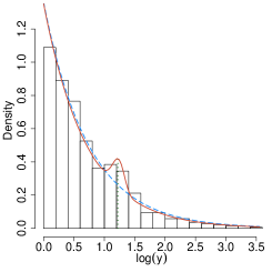
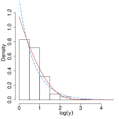
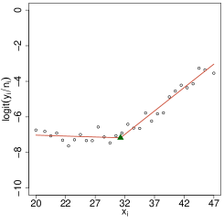
Figure 1: Data and fitted models. Left panel: histogram of the Fermi-LAT realistic data simulation for Example 1 (on $log$-scale), null model (blue dashed curve) fitted under the assuption of background only counts ($\hat{\phi}=1.350$), and fitted alternative model (red solid curve) with $\hat{\eta}=0.045$, $\hat{\phi}=1.406$. The green dotted vertical line indicates the location of the observed Gaussian bump, i.e., $\hat{\theta}=3.404$. Central panel: histogram of the Fermi-LAT realistic data simulation for Example 2 ($log$-scale), the null model when testing (1.2) is fitted as a power-law distributed cosmic source with $\hat{\phi}=1.395$ (blue dashed curve). The null model when testing (3.16) is the dark matter model in (3.14) with $\hat{\theta}=27.89$ obtained via MLE (red solid curve) . Right panel: Down syndrome data and fitted regression model (red piecewise-linear solid lines), with break-point (green triangle) at $\hat{\theta}=31.266$.

3 Practical matters

3.1 Case studies: description

Here we illustrate the implementation of TOHM in the context of three case studies, i.e., the “bump hunting” problem introduced in Section 1, a non-nested models comparison, and a logistic model with a break point. Hereafter, we refer to these as Examples 1, 2 and 3, respectively. Data for Examples 1 and 2 were generated using simulations of the Fermi Large Area Telescope (LAT) obtained with the gtobssim package and include representations of detector effects and systematic errors. The Fermi-LAT is a $\gamma$-ray telescope on the orbiting Fermi satellite (Atwood et al., 2009).

In Example 1, our data analysis aims to properly distinguish between $\gamma$-ray signals induced by dark matter annihilations and those induced by the astrophysical background. As in (1.1), dark matter events are modeled as a Gaussian bump with mean energy $\theta$ and standard deviation varying with $\theta$. The astrophysical background is power-law (Pareto type I) distributed with index $\phi$. In our simulation, we set $\theta=3.5$GeV (where GeV denotes Giga electron-volt), $\phi=1.4$, $\eta=0.02$, and we consider the energy band $y\in[1;35]$. This setup resulted in 64 dark matter events and 2274 background events. For more physics details, see Algeri et al. (2016).

In Example 2, the non-nested models to be compared are a dark matter emission with probability density given by

$$g(y,\theta)\propto y^{-1.5}\exp\biggl{\{}-7.8\frac{y}{\theta}\biggl{\}},$$ (3.14)

with $y\geq 1$, $\phi>0$ and $\theta\geq 1$ (see Bergström et al., 1998) and a power-law distributed cosmic source with density $f(y,\phi)\propto\frac{1}{k_{\phi}y^{\phi+1}}$. In our simulation we set the putative dark matter emission to occur at $\theta=35$GeV, and the power-law index to $\phi=1.4$. In this way, we obtained 200 dark matter events over the energy band $y\in[1;100]$.

Since the models $f(y,\phi)$ and $g(y,\theta)$ are non-nested, the classical asymptotic properties of the MLE and LRT fail. However, as shown in Algeri et al. (2016), the framework of Section 2 can be extended to compare non-nested models by reformulating this comparison as a test in which a nuisance parameter is identified only under $H_{1}$. Specifically, following Cox (1962) and Atkinson (1970), we specify a comprehensive model that embes two non-nested models, i.e.,

$$(1-\eta)f(y,{\phi})+\eta g(y,\theta)\qquad 0\leq\eta\leq 1.$$ (3.15)

This reduces the problem to a nested models comparison and we test (1.2). However, in contrast to the bump-hunting example in (1.1), here $\eta$ has no physical interpretation. Rather, as in Quandt (1974), $\eta$ is an auxiliary parameter which allows us to exploit the normality of its MLE to apply well-know asymptotic results. In addition to (1.2), the hypotheses

$$H_{0}:\eta=1\quad\mbox{versus}\quad H_{1}:\eta<1$$ (3.16)

should also be tested in order to exclude intermediate situations (e.g., Cox, 1962, 2013). I.e., we want to avoid treating (3.15) as a mixture and focus on comparing the two models. Testing both (1.2) and (3.16) is particularly suited to particle physics searches where researchers typically assign different degrees of belief to the models being tested. Specifically, as described in van Dyk (2014), the most stringent significance requirements (e.g., Lyons, 2013, Table 1) are typically used only in the detection stage, i.e., when testing (1.2) to assess the presence of a new signal. Conversely, in the exclusion stage, i.e., when testing (3.16) to exclude the hypothesis of a signal being present, a significance level of 0.05 is typically sufficient. The Fermi-LAT datasets for Examples 1 and 2 are plotted in the first two panels of Figure 1. Both simulations are downloadable among the Supplementary Materials.

Finally, in Example 3 we consider the Down Syndrome dataset available in the R package egmented \citep{egmented. The dataset records whether babies born to 354,880 women are affected by Down Syndrome. We use (317) to model the probability, $\pi_{i}$, that a woman of age $x_{i}$ has a baby with down syndrome, where $x_{i}\in[17;47]$, and we let $\theta\in[20;44]$. The logit of the ratio between the number of down syndrome cases and number of births by age group is plotted in the right panel of Figure 1.

$$\log\biggl{(}\frac{\pi_{i}}{1-\pi_{i}}\biggl{)}=\phi_{1}+\phi_{2}x_{i}+\xi(x_{i}-\theta)\mathbbm{1}_{\{x_{i}\geq\theta\}}\quad\forall i=1,\dots,n,$$ (317)

where $\theta\in\mathbb{R}$ is the location of the unknown break-point. In this case, we test $H_{0}:\xi=0$ versus $H_{1}:\xi\neq 0$. In Example 1 and 2 we use the LRT, $T_{n}(\theta)$, as the sub-test statistic. Since both tests are of the form in (1.2), the test is on the boundary of the parameter space and for each $\theta$ fixed the asymptotic distribution under $H_{0}$ is a mixture of $\chi_{1}^{2}$ and zero (Chernoff, 1954; Self and Liang, 1987), also known as $\bar{\chi}$-distribution and which we dentote with $\bar{\chi}^{2}_{01}$. It can be shown (Algeri and van Dyk, 2018) that in this setting the bound in (2.8) has the same form as in the $\chi^{2}_{1}$ case, i.e., it is given by (1.5) with $s=1$. In Example 3, we use the signed-root of the LRT $Q_{n}(\theta)=\text{sign}(\hat{\eta}_{\theta}-\eta_{0})\sqrt{T_{n}(\theta)}$, hence the sub-tests statistics are asymptotically normally distributed under $H_{0}$ (e.g., Davies, 1977).

3.2 The choices of $c_{0}$ and $R$

One way to select an appropriate thresholds $c_{0}$ is to perform a sensitivity analysis based on few Monte Carlo simulations of the traces of the underlying processes under $H_{0}$. As discussed in Section 2, under suitable regularity conditions and when $H_{0}$ is true, the LRT and signed-root LRT processes $\{T_{n}(\theta)\}$ and $\{Q_{n}(\theta)\}$ converge uniformly to $\{W_{\chi}(\theta)\}$ and $\{Z(\theta)\}$, respectively, as $n\rightarrow+\infty$. More generally, given a test statistics $W_{n}(\theta)$ to be evaluated on the data $y_{1},\dots,y_{n}$ for each $\theta$ fixed, we write $\{W_{n}(\theta)\}\xrightarrow{d}\{W(\theta)\}$. Consequently, for each sample generated under $H_{0}$, we compute $\{W_{n}(\theta)\}$ over a fine grid of values of $\theta$ and which approximates $\{W(\theta)\}$ when $n$ is large. In all our simulations, the nuisance parameters under the null model have been estimated via MLE and each simulated sample under $H_{0}$ is obtained via parametric bootstrap (Efron and Tibshirani, 1994). We plot the results of our simulation in order to visualize the traces of $\{W_{n}(\theta)\}$ as shown in Figure 2 for Example 1. (The analogous plots for Examples 2 and 3 appear in Figure LABEL:upc_others.) In order to calculate (2.8), it is important to provide an accurate estimate of $E[N_{c_{0}}]$. Hence, we choose $c_{0}$ to be at a level (on the y-axis) around which the process $\{W_{n}(\theta)\}$ oscillates often, and thus, with respect to which the upcrossings occur with high frequency. For Examples 1, 2 and 3, this leads to values $c_{0}$ equal to $0.1,0.3$ and $0$, respectively. Inspecting the smoothness of the trace plots also allows us to qualitatively assess Condition 1 and verify the goodness of the approximation of $E[N_{c_{0}}]$ by $E[\tilde{N}_{c_{0}}]$, necessary for the validity of the results of Section 2.

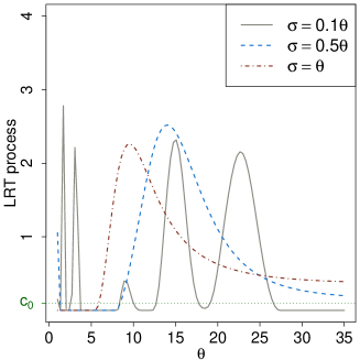
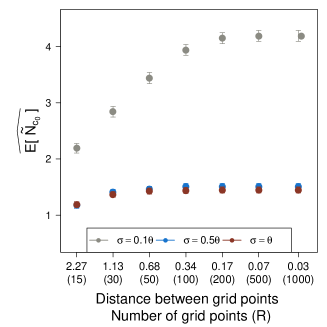
Figure 2: Left panel: simulated sample paths of the LRT process, $\{T_{n}(\theta)\}$, under $H_{0}$ in Example 1. Both plots consider different widths of the Gaussian bump. Right panel: upcrossings plot showing Monte Carlo estimates of $E[\tilde{N}_{c_{0}}]$ and standard errors (whiskers), under $H_{0}$, for Example 1, and evaluated over grids of $R=15,30,50,100,200,500$ points, and for three choices of the Gaussian width, namely $\sigma=0.1\theta,\sigma=0.5\theta$ and $\sigma=\theta$.

As discussed in Section 1, the implementation of our procedure requires the specification of a grid $\Theta_{R}$ over $\Theta\equiv[\mathcal{L};\mathcal{U}]$, where $R$ is the number of times $H_{0}$ is tested versus the ensemble of sub-alternatives $H_{11},\dots,H_{1R}$. In practice, $R$ must either be chosen arbitrarily by the researcher or determined by the nature of the experiment. In either case, $R$ must be sufficiently large to guarantee robustness of the results, yet small enough to ensure computational efficiency when calculating (2.13). One possibility is to choose $R$ large enough so that, for a given $c_{0}$, $E[\tilde{N}_{c_{0}}]$ converges to a finite limit, which we expect, for sufficiently dense $\Theta_{R}$, to correspond to $E[N_{c_{0}}]$. This strategy requires us to set $c_{0}$ before setting $R$. In order to identify the value of $R$ that best negotiates the trade-off between accuracy and computational efficiency, one can consider different values of $R$ and for each of them compute an estimate of $E[{N}_{c_{0}}]$ by means of a small Monte Carlo simulation. The results can then be summarized in an upcrossing plot where the values for $R$ considered are reported on the $x$-axis and the respective $\widehat{E[\tilde{N}_{c_{0}}]}$ estimates of $E[{N}_{c_{0}}]$ are reported on the $y$-axis. The upcrossing plot in the right panel of Figure 2 displays Monte Carlo estimates $\widehat{E[\tilde{N}_{c_{0}}]}$ for the LRT in Example 1, under $H_{0}$, as a function of $R$ (with $R=15,30,50,100,200,500,1000$). For each value of $R$ considered, the grid points have been chosen to be equally spaced over $\Theta$. Analogous plots for Examples 2 and 3 appear in Figure LABEL:upc_others. For each $R$ considered we computed 100 Monte Carlo simulations, each of size 1000. In all our examples, 100 simulations are sufficient to achieve small Monte Carlo errors. As a rule of thumb, if the number of upcrossings increases with $R$ but does not converge, it means that the resolution is not sufficiently high to catch all the crossings or, the underlying process is not sufficiently smooth to guarantee $E[{N}_{c_{0}}]<\infty$. Conversely, if the number of upcrossings converges, as in the well-known scree-plot used for Principal Component Analysis (PCA) (e.g., James et al., 2013, p. 383), we look for an “elbow” in the plot of $\widehat{E[\tilde{N}_{c_{0}}]}$. The value of $R$ corresponding to the elbow is the smallest value for which $\widehat{E[\tilde{N}_{c_{0}}]}$ converges to its limit, $E[{N}_{c_{0}}]$, up to Monte Carlo error. In physics terms, this corresponds to the minimal value of $R$ for which $\widehat{E[\tilde{N}_{c_{0}}]}$ well approximates the number of upcrossings of the underlying continuous time process.

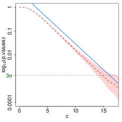
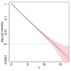
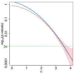
Figure 3: Estimated bound/approximation in (2.13) (blue solid line), simulated global p-values (on $\log_{10}$-scale), Monte Carlo estimates of $P(\sup_{\theta\in\Theta}\{W(\theta)\}>c)$ (red dashed line), and Monte Carlo Errors (pink areas) for increasing values of the threshold $c$, for Example 1 (left panel), Example 2 (central panel) and Example 3 (right panel). Monte Carlo errors associated with $\widehat{E[\tilde{N}_{c_{0}}]}$ on the bound in (2.13) are plotted in grey, but are too small to be visible.

We also investigate the relationship between the width of the signal in the bump-hunting example, and the grid resolution. In particular, we replicate the simulation for three choices of the Gaussian width, namely $\sigma=0.1\theta,\sigma=0.5\theta$ and $\sigma=\theta$. (In our actual analysis $\sigma=0.1\theta$.) As expected, wider signals correspond to smoother underlying processes (Figure 2, left panel) and $\widehat{E[\tilde{N}_{c_{0}}]}$ converges (Figure 2, right panel) at lower grid resolution. In general, $R$ impacts the upper bound/approximation for the global p-value in (2.8), as well as the observed value of the test statistics, $c_{R}$, which we assume converges to $c$, as $R\rightarrow\infty$. Specifically, if the gap between $\theta_{r}$ and $\theta_{r+1}$ is wider than the signal width, $c_{R}$ may underestimate $c$, and the signal may be missed. Thus, if the signal is suspected to be localized over a small region of the search interval, a higher resolution is required to accurately estimate (2.13) and avoid false negatives, which would in turn adversely affect the power of the test. Conversely, in Examples 2 and 3, the signal is spread either over the whole parameter space or over a large portion of it. In these cases the choice of $R$ should be based on the desired level of accuracy of both $c_{R}$ as an estimate for the maximum of the underlying process and of the value of $\theta$ at which the maximum occurs, i.e.,

$$\tilde{\theta}=\text{argmax}_{\theta_{r}\in\Theta_{R}}\{W(\theta_{r})\}.$$ (318)

Finally, based on the elbow in the upcrossing plots in Figures 2 and LABEL:upc_others, the values of $R$ we select are $R=100$ in Example 1 (with $\sigma=0.1\theta$ as in (1.1)), $R=50$ in Example 2, and $R=30$ in Example 3. In order to guarantee accuracy of at least $0.5$ for the identified location, $\tilde{\theta}$, of the break-point, however, we set $R=50$ in Example 3. For each of the models considered, we computed (2.13) using the $R$ and $c_{0}$ selected above. The results obtained are compared in Figure 3 with the Monte Carlo estimates of $P(\sup_{\theta\in\Theta}\{W(\theta)\}>c)$ for increasing values of $c$, obtained using 100,000 simulations, each of size 10,000. The pink areas correspond to the respective Monte Carlo errors. The Monte Carlo errors associated to the estimate $\widehat{E[\tilde{N}_{c_{0}}]}$ for $E[\tilde{N}_{c_{0}}]$ in (2.13) (and displayed on a lower scale in the upcrossing plots) are also incorporated in Figure 3, but they are too small to be visible. As expected, the estimated TOHM bounds approach the “truth” as $c\rightarrow\infty$. Convergence appears to be slower for Example 1. The plots, however, are presented on $\log_{10}$-scale, and thus in all cases we obtain a good approximations of the global p-values.

4 Comparing TOHM and Bonferroni’s bounds

In fields such as high energy physics and astrophysics, experiments are often characterized by the search of one signal over a wide pool of possibilities. The simplest possible way to tackle this problem using classical Multiple Hypothesis Testing (MHT) is by means of Bonferroni correction (Bonferroni, 1935, 1936). The Bonferroni bound for the global p-value is

$$p_{\mathrm{B}F}=R\cdot\min_{\theta_{r}\in\Theta_{R}}P(W(\mathcal{L})\geq w(\theta_{r}))=R\cdot P(W(\mathcal{L})\geq c_{R}).$$ (419)

The standard Bonferoni correction, $p_{\mathrm{B}F}$, used to bound statistical significance in multiple testing also yields a bound on $P(\max_{\theta_{r}\in\Theta_{R}}\{W(\theta_{r})\}\geq c_{R})$. Specifically,

$$P\biggl{(}\max_{\theta_{r}\in\Theta_{R}}\{W(\theta_{r})\}\geq c_{R}\biggl{)} =P\biggl{(}\cup_{\theta_{r}\in\Theta_{R}}\{W(\theta_{r})>c_{R}\}\biggl{)}\leq\sum_{\theta_{r}\in\Theta_{R}}P(W(\theta_{r})>c_{R})$$

$$=R\cdot P(W(\mathcal{L})>c_{R})=p_{BF}.$$

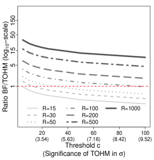
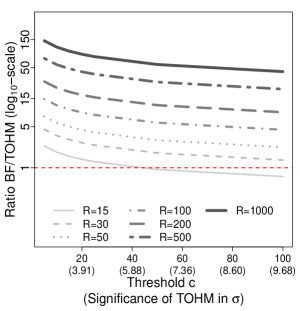
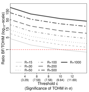
Figure 4: Ratio of Bonferroni and TOHM’s bounds at increasing values of $c$ (and corresponding significance for TOHM), and considering different resolutions (grey curves). The left, central and right panels correspond to Example 1, 2 and 3, respectively.

In this section, we investigate the relationship between the TOHM and Bonferroni bounds using simple constructs from EVT in order to individuate situations where the latter can be used without leading to overly conservative results. First, we introduce the distinction between upcrossings and exceedances of $\{W(\theta_{r})\}$. Specifically, an exceedance of $c_{R}$ by $\{W(\theta_{r})\}$ occurs at $\theta_{r}$ if $\{W(\theta_{r})>c_{R}\}$. An illustration of the difference between upcrossings and exceedances is given in Figure LABEL:exceedances. We denote by $\tilde{N}_{c_{R}}$, the process of exceedances of $c_{R}$ by $\{W(\theta_{r})\}$, and let $\dot{N}_{c_{R}}$ be the process of upcrossings as defined in 2.3. Notice that

$$E[\dot{N}_{c_{R}}] =\sum^{R}_{r=1}P\biggl{(}W(\theta_{r})\geq c_{R}\biggl{)}=\sum^{R}_{r=1}P\biggl{(}W(\theta_{r})\geq\max_{\theta_{r^{\prime}}\in\Theta_{R}}\{w(\theta_{r^{\prime}})\}\biggl{)}$$ (420)

$$=R\min_{\theta_{r}\in\Theta_{R}}P(W(\mathcal{L})\geq w(\theta_{r}))=p_{\mathrm{B}F}$$ (421)

Because each upcrossing requires at least one exceedance, $E[\dot{N}_{c_{R}}]\geq E[\tilde{N}_{c_{R}}]$. Moreover, we expect that the clusters of exceedances corresponding to each upcrossing to be smaller, and consequently $E[\dot{N}_{c_{R}}]$ to approach $E[\tilde{N}_{c_{R}}]$ as $c_{R}$ increases. $E[\dot{N}_{c_{R}}]$ can be easily computed using $p_{\mathrm{B}F}$ in (420)-(421); whereas, when $\{W(\theta)\}$ satisfies Condition 1, $E[\tilde{N}_{c_{R}}]$ is approximately equal to the second term in (2.13), for large $R$. Further, $E[\tilde{N}_{c_{R}}]$ dominates the first term in (2.13), as $c_{R}\rightarrow\infty$. Thus, it is natural to consider if there are situations where $\eqref{real_bound}$ and $p_{\mathrm{B}F}$ are approximately equivalent bounds on $P(\max_{\theta_{r}\in\Theta_{R}}\{W(\theta_{r})\}\geq c_{R})$, i.e,

$$P(W(\mathcal{L})>c_{R})+\frac{a(c_{R})}{a(c_{0})}E[\tilde{N}_{c_{0}}]\approx p_{\mathrm{B}F},$$ (422)

for $c_{0}\leq c_{R}$, $c_{R}\rightarrow+\infty$ and $R\rightarrow+\infty$. Unfortunately, simultaneously quantifying the rates at which $c_{R}$ and $R$ must increase for (422) to hold is not an easy task; hence, we investigate the approximation in (422) by means of a numerical simulation where we compare the performance of Bonferroni and the TOHM bounds with respect to the number of tests considered and the level of significance for Examples 1, 2 and 3. The results are reported in Figure 4, where we plot the ratio of the two bounds for increasing values of $c$, using different grid sizes, $R$. Because the signed-root LRT, $\{Q_{n}(\theta)\}$, is used in Example 3 rather than the LRT, smaller values of $c$ correspond to equally significant results. In the horizontal axes, the statistical significance is reported in terms of $\sigma$-significance, i.e., the number of standard deviations from the mean of a standard normal distribution that corresponds to the tail probability expressed by the one-sided p-value, i.e.,

$$\#\sigma=\Phi^{-1}(1-\text{p-value}),$$

where $\Phi$ is the standard normal cumulative function. In Examples 2 and 3, Bonferroni is always more conservative than the TOHM bound when at least 30 tests are performed. For $R=15$, Bonferroni becomes less conservative only when the level of significance achieved is of the order of $6\sigma$ and $11\sigma$, respectively. A more interesting situation is observed for Example 1. Here, equivalence of $p_{\mathrm{T}OHM}$ and $p_{\mathrm{B}F}$ occurs for values of $c$ much smaller than those for which the same limit is achieved in Examples 2 and 3. Further, when $R\leq 50$, Bonferroni quickly becomes less conservative than the TOHM bound as $c$ increases. For $R=50$ for instance, Bonferroni performs better than TOHM when $c>30$ ($\sim 4.5\sigma$ significance). Finally, all the plots in Figure 4 suggest that the TOHM bound is preferable to Bonferroni with very high resolutions, i.e. $R\geq 500$, for all the significance levels considered (up to $\sim 10\sigma$). It is important to point out that the value of $R$ selected via the upcrossing plots discussed in Section 3.2 is the minimum number of grid points (among those considered) for which $\widehat{E[\tilde{N}_{c_{0}}]}$ converges to its limit. As $R$ increases beyond this point, the estimated TOHM bound remains constant, whereas Bonferroni’s continues to increase. This implies that, when the number of tests to be conducted can be selected arbitrarly, Bonferroni will not be overly conservative if the “elbow” in the upcrossings plot appears at a relatively small value of $R$ and the observed value of $c$ is large. However, practitioners should keep in mind that when attempting to identify the signal location, $\tilde{\theta}$, a higher resolution is typically required and thus TOHM is preferable.

Example	Test	Method	$R$	$c_{R}$	$\tilde{\theta}$	p-value
						(Significance)
Example 1	$H_{0}:\eta=0$	Bonferroni	100	38.326	3.404	$2.99\cdot 10^{-8}$ ($5.42\sigma$)
	$H_{1}:\eta>0$	TOHM				$2.11\cdot 10^{-8}$ ($5.48\sigma$)
Example 2	$H_{0}:\eta=0$	Bonferroni	50	21.021	27.265	$1.14\cdot 10^{-4}$ ($3.69\sigma$)
	$H_{1}:\eta>0$	TOHM				$2.51\cdot 10^{-5}$ ($4.06\sigma$)
	$H_{0}:\eta=1$	Bonferroni	50	0.606	27.890	$>1$ ($0.00\sigma$ )
	$H_{1}:\eta<1$	TOHM				$7.201\cdot 10^{-1}$ ($0.58\sigma$)
Example 3	$H_{0}:\xi=0$	Bonferroni	50	11.826	31.266	$1.43\cdot 10^{-30}$ ($11.43\sigma$)
	$H_{1}:\xi\neq 0$	TOHM				$5.06\cdot 10^{-31}$ ($11.52\sigma$)

Table 1: Summary of the results of TOHM and MHT via Bonferroni on real data for Examples 1, 2 and 3.

4.1 Data analyses

In this section we compare the TOHM and Bonferroni bounds for Examples 1, 2 and 3. The results are summarized in Table 1. In the dark matter search problem of Example 1, we obtain a significance in favour of the presence of a dark matter emission of about $5.4\sigma$ using both TOHM and MHT. This result is not surprising since $c_{R}=38.326$ and as shown in the central panel of Figure 4, at $c\approx 40$ the gray line associated with $R=100$ is very close the red dashed line. The signal location selected is close to the truth (3.5GeV), and the estimated model is plotted as a solid red line in the left panel of Figure 1; the signal location selected, $\tilde{\theta}=3.404$, is indicated by the green dotted vertical line. In Example 2 both TOHM and Bonferroni reject the hypothesis that the observed emission is due to a power-law distributed cosmic source at $4.06\sigma$ and $3.69\sigma$ respectively. Because this example involves a non-nested models comparison, we invert the null of the hypotheses in order to avoid meaningless results (see Section 3.1 for more details). In the inverted test, the power-law model cannot be rejected. Both the fitted dark matter model and the fitted power-law cosmic source model are displayed in the central panel of Figure 1. In Example 2, when testing (1.2), the value of $\theta$ (i.e., the signal annihilation of the dark matter model) selected by TOHM is $\tilde{\theta}=27.265$GeV. This is somewhat off from the true value used to simulate the data ($\theta=35$GeV), perhaps because our analysis does not account for instrumental errors. Our analysis also only uses the spectral energy of the $\gamma$-ray signals, whereas in practice the directions of the $\gamma$-ray would also be used, thus increasing the statistical power. Finally, for the break-point regression model in Example 3, both TOHM and MHT give similar inferences ($11.52\sigma$ and $11.43\sigma$ respectively) when rejecting the hypothesis of a linear model with no break-point. The equivalence among the two procedure is likely due to the very high statistical significance, and the only moderately large number of tests conducted ($R=50$). The fitted model is displayed in Figure 1 where the green triangle corresponds to the optimal break-point location, i.e., the maximum of the signed-root LRT process occurs at a mother’s age of 31.266 years.

5 Discussion

In this paper we discuss a highly generalizable method to efficiently conduct statistical tests under non-standard conditions, including bump-hunting, structural change detection and non-nested models comparison. The main advantages of the method proposed are its easy implementation and its efficiency in providing accurate inference, while controlling for very small Type I errors rates. Following Davies (1987) and Gross and Vitells (2010) we combine the theoretical framework of EVT with the practical simplicity of Monte Carlo simulations and we generalize their results beyond the LRT and $\chi^{2}$. Using a suite of simulation studies we show that as few as 100 Monte Carlo simulations are often sufficient to achieve a high level of accuracy. Although we do not investigate the power of TOHM here, readers interested in power are directed to Davies (1977) for a formal derivation of lower and upper bounds of the power function in the normal case, or the simulation studies conducted in Algeri et al. (2016) and Algeri et al. (2016) for the $\bar{\chi}^{2}_{01}$ case. From a more practical perspective, we propose simple graphical tools to select the threshold $c_{0}$ and to specify an appropriate number of sub-tests $R$ to guarantee robustness of the resulting inference. Finally, we investigate the relationship between the TOHM and Bonferroni bounds and we implement both procedures on our running examples. Extensions of our results to the case where the nuisance parameter specified only under the alternative, ${\bm{\theta}}$, is multi-dimensional are the subject of a forthcoming paper (Algeri and van Dyk, 2018). It is important to point out that the stringent significance requirements play a critical role in both the theory discussed in Section 2 and practical applications. Specifically, this setup is particularly well suited for searches in high energy physics, where the significance level necessary to claim a discovery is of at least $5\sigma$. However, in light of the recent “p-value crisis”, culminated with the Journal Basic and Applied Social Psychology banning the use of the p-value in future submissions (Wasserstein and Lazar, 2016; Leek and Peng, 2015), stringent significance criteria may become more popular in other scientific communities.

Supplementary Materials In Section S.1 we discuss the error rate of (2.8) for Gaussian, $\chi^{2}$ and $\bar{\chi}^{2}_{01}$ processes. Proofs of Result 2 and Result 3 are collected in Section S.2. Additionally figures are reported in Section S.3. Data used in Examples 1 and 2 are also downloadable among the Supplementary Materials.

Acknowledgements The authors thank two anonymous referees and the associate editor for their constructive feedback. SA and DvD also thank Jan Conrad for the valuable discussion of the physics problems which motivated this work, and Brandon Anderson who provided the Fermi-LAT datasets used in the analyses. DvD acknowledges support from Marie-Skodowska-Curie RISE (H2020-MSCA-RISE-2015-691164) Grant provided by the European Commission.

Sara Algeri
School of Statistics
University of Minnesota
Minneapolis, MN, 55455 E-mail: salgeri@umn.edu David van Dyk
Statistics Section
Dept of Mathematics
Imperial College London
London, UK SW7 2AZ E-mail: d.van-dyk@imperial.ac.uk

References

- Adler (2000) Adler, R. (2000). On excursion sets, tube formulas and maxima of random fields. Annals of Applied Probability, 1–74.
- Adler and Taylor (2009) Adler, R. and J. Taylor (2009). Random fields and geometry. Springer Science & Business Media.
- Algeri et al. (2016) Algeri, S. et al. (2016). On methods for correcting for the look-elsewhere effect in searches for new physics. Journal of Instrumentation 11(12), P12010.
- Algeri et al. (2016) Algeri, S., J. Conrad, and D. van Dyk (2016). A method for comparing non-nested models with application to astrophysical searches for new physics. Monthly Notices of the Royal Astronomical Society: Letters 458(1), L84–L88.
- Algeri and van Dyk (2018) Algeri, S. and D. van Dyk (2018). Testing one hypothesis multiple times: The multidimensional case. arXiv:1803.03858.
- Anderson et al. (2016) Anderson, B. et al. (2016). Search for gamma-ray lines towards galaxy clusters with the fermi-lat. Journal of Cosmology and Astroparticle Physics 2016(02), 026.
- Andrews (1993) Andrews, D. (1993). Tests for parameter instability and structural change with unknown change point. Econometrica: Journal of the Econometric Society, 821–856.
- Andrews and Ploberger (1994) Andrews, D. and W. Ploberger (1994). Optimal tests when a nuisance parameter is present only under the alternative. Econometrica: Journal of the Econometric Society, 1383–1414.
- Atkinson (1970) Atkinson, A. (1970). A method for discriminating between models. Journal of the Royal Statistical Society. Series B (Methodological), 323–353.
- Atwood et al. (2009) Atwood, W. B. et al. (2009). The large area telescope on the fermi gamma-ray space telescope mission. The Astrophysical Journal 697(2), 1071.
- Bergström et al. (1998) Bergström, L., P. Ullio, and J. Buckley (1998). Observability of rays from dark matter neutralino annihilations in the milky way halo. Astroparticle Physics 9(2), 137–162.
- Bonferroni (1935) Bonferroni, C. (1935). Il calcolo delle assicurazioni su gruppi di teste. In Studi in Onore del Professore Salvatore Ortu Carboni, pp. 13–60. Rome.
- Bonferroni (1936) Bonferroni, C. (1936). Teoria statistica delle classi e calcolo delle probabilità. Pubblicazioni del R Istituto Superiore di Scienze Economiche e Commerciali di Firenze 8, 3–62.
- Chernoff (1954) Chernoff, H. (1954). On the distribution of the likelihood ratio. The Annals of Mathematical Statistics, 573–578.
- Choudalakis (2011) Choudalakis, G. (2011). On hypothesis testing, trials factor, hypertests and the BumpHunter. In Proceedings, PHYSTAT 2011. ArXiv:1101.0390.
- Cox (1962) Cox, D. (1962). Further results on tests of separate families of hypotheses. Journal of the Royal Statistical Society. Series B (Methodological), 406–424.
- Cox (2013) Cox, D. (2013). A return to an old paper:‘tests of separate families of hypotheses’. Journal of the Royal Statistical Society: Series B (Statistical Methodology) 75(2), 207–215.