11institutetext: LIG - CNRS and Université de Grenoble Alpes, France
11email: rachid.echahed@imag.fr
22institutetext: LJK - Université de Grenoble Alpes and CNRS, France
22email: aude.maignan@imag.fr

Parallel Graph Rewriting with Overlapping Rules

Rachid Echahed 11    Aude Maignan 22
Abstract

We tackle the problem of simultaneous transformations of networks represented as graphs. Roughly speaking, one may distinguish two kinds of simultaneous or parallel rewrite relations over complex structures such as graphs: (i) those which transform disjoint subgraphs in parallel and hence can be simulated by successive mere sequential and local transformations and (ii) those which transform overlapping subgraphs simultaneously. In the latter situations, parallel transformations cannot be simulated in general by means of successive local rewrite steps. We investigate this last problem in the framework of overlapping graph transformation systems. As parallel transformation of a graph does not produce a graph in general, we propose first some sufficient conditions that ensure the closure of graphs by parallel rewrite relations. Then we mainly introduce and discuss two parallel rewrite relations over graphs. One relation is functional and thus deterministic, the other one is not functional for which we propose sufficient conditions which ensure its confluence.

0.1 Introduction

Graph structures are fundamental tools that help modeling complex systems. In this paper, we are interested in the evolution of such structures whenever the dynamics is described by means of systems of rewrite rules. Rewriting techniques are being investigated for different structures such as strings [4], trees [1] or graphs [20]. Roughly speaking, a rewrite rule can be defined as a pair lr𝑙𝑟l\to r where the left-hand and the right-hand sides are of the same structure. A rewrite system, consisting of a set of rewrite rules, induces a rewrite relation (\to) over the considered structures. The rewrite relation corresponds to a sequential application of the rules, that is to say, a structure G𝐺G rewrites into a structure Gsuperscript𝐺G^{\prime} if there exits a rule lr𝑙𝑟l\to r such that l𝑙l occurs in G𝐺G. Then Gsuperscript𝐺G^{\prime} is obtained from G𝐺G by replacing l𝑙l by r𝑟r.

Besides this classical rewrite relation, one may think of a parallel rewrite relation which rewrites a structure G𝐺G into a structure Gsuperscript𝐺G^{\prime} by firing, simultaneously, some rules whose left-hand sides occur in G𝐺G. Simultaneous or parallel rewriting of a structure G𝐺G into Gsuperscript𝐺G^{\prime} can be used as a means to speed up the computations performed by rewrite systems and, in such a case, parallel rewriting can be simulated by successive sequential rewrite steps. However, there are situations where parallel rewrite steps cannot be simulated by sequential steps as in formal grammars [11], cellular automata (CA) [23] or L-systems [19]. This latter problem is of interest in this paper in the case where structures are graphs.

Graph rewriting is a very active area where one may distinguish two main stream approaches, namely (i) the algorithmic approaches where transformations are defined by means of the actual actions one has to perform in order to transform a graph, and (ii) the algebraic approaches where graph transformations are defined in an abstract level using tools borrowed from category theory such as pushouts, pullbacks etc. [20]. In this paper, we introduce a new class of graph rewrite systems following an algorithmic approach where rewrite rules may overlap. That is to say, in the process of graph transformation, it may happen that some occurrences of left-hand sides of different rules can share parts of the graph to be rewritten. This overlapping of the left-hand sides, which can be very appealing in some cases, turns out to be a source of difficulty to define rigorously the notion of parallel rewrite steps. In order to deal with such a difficulty we follow the rewriting modulo approach (see, e.g. [16]) where a rewrite step can be composed with an equivalence relation. Another complication comes from the fact that a graph can be reduced in parallel in a structure which is not always a graph but rather a structure we call pregraph. Thus, we propose sufficient conditions under which graphs are closed under parallel rewriting. The rewrite systems we obtain generalize some known models of computation such as CA, L-systems and more generally substitution systems [23]. As a simple example illustrating this work, we may refer to mesh refinement [5] and adaptative mesh refinement (AMR) which constitute a very usefull technique in physics [3, 17], astrophysics [12, 6] or in biology [18].

The paper is organized as follows. The next section introduces the notions of pregraphs and graphs in addition to some preliminary results linking pregraphs to graphs. In Section 0.3, a class of rewrite systems, called environment sensitive rewrite systems is introduced together with a parallel rewrite relation. We show that graphs are not closed under such rewrite relation and propose sufficient conditions under which the outcome of a rewrite step is always a graph. Then, in Section 0.4, we define two particular parallel rewrite relations, one performs full parallel rewrite steps whereas the second relation uses the possible symmetries that may occur in the rules and considers only matches up to automorphisms of the left-hand sides. Section 0.5 illustrates our framework through some examples. Concluding remarks and related work are given in Section 0.6.

0.2 Pregraphs and Graphs

In this section we first fix some notations and give preliminary definitions and properties. 2Asuperscript2𝐴2^{A} denotes the power set of A. AB𝐴𝐵A\uplus B stands for the disjoint union of two sets A𝐴A and B𝐵B. In the following, we introduce the notion of (attributed) pregraphs, which denotes a class of structures we use to define parallel graph transformations. Elements of a pregraph may be attributed via a function λ𝜆\lambda which assigns, to elements of a pregraph, attributes in some sets which underly a considered attributes’ structure 𝒜𝒜{\cal A}. For instance 𝒜𝒜{\cal A} may be a ΣΣ\Sigma-algebra [21] or merely a set.

Definition 1 (Pregraph).

A pregraph H𝐻H is a tuple H=(𝒩H,𝒫H,𝒫𝒩H,𝒫𝒫H,𝒜H,λH)𝐻subscript𝒩𝐻subscript𝒫𝐻𝒫subscript𝒩𝐻𝒫subscript𝒫𝐻subscript𝒜𝐻subscript𝜆𝐻H=({\cal N}_{H},{\cal P}_{H},{\cal PN}_{H},{\cal PP}_{H},{\cal A}_{H},\lambda_{H}) such that :

  • 𝒩Hsubscript𝒩𝐻{\cal N}_{H} is a finite set of nodes and 𝒫Hsubscript𝒫𝐻{\cal P}_{H} is a finite set of ports,

  • 𝒫𝒩H𝒫subscript𝒩𝐻{\cal PN}_{H} is a relation 𝒫𝒩H𝒫H×𝒩H𝒫subscript𝒩𝐻subscript𝒫𝐻subscript𝒩𝐻{\cal PN}_{H}\subseteq{\cal P}_{H}\times{\cal N}_{H},

  • 𝒫𝒫H𝒫subscript𝒫𝐻{\cal PP}_{H} is a symmetric binary relation on ports, 𝒫𝒫H𝒫H×𝒫H𝒫subscript𝒫𝐻subscript𝒫𝐻subscript𝒫𝐻{\cal PP}_{H}\subseteq{\cal P}_{H}\times{\cal P}_{H},

  • 𝒜Hsubscript𝒜𝐻{\cal A}_{H} is a structure of attributes,

  • λHsubscript𝜆𝐻\lambda_{H} is a function λH:𝒫H𝒩H2𝒜H:subscript𝜆𝐻subscript𝒫𝐻subscript𝒩𝐻superscript2subscript𝒜𝐻\lambda_{H}:{\cal P}_{H}\uplus{\cal N}_{H}\rightarrow 2^{{{\cal A}_{H}}} such that x𝒩H𝒫H,card(λH(x))for-all𝑥subscript𝒩𝐻subscript𝒫𝐻𝑐𝑎𝑟𝑑subscript𝜆𝐻𝑥\forall x\in{\cal N}_{H}\uplus{\cal P}_{H},card(\lambda_{H}(x)) is finite.

An element (p,n)𝑝𝑛(p,n) in 𝒫𝒩H𝒫subscript𝒩𝐻{\cal PN}_{H} means that port p𝑝p is associated to node n𝑛n. An element (p1,p2)subscript𝑝1subscript𝑝2(p_{1},p_{2}) in 𝒫𝒫H𝒫subscript𝒫𝐻{\cal PP}_{H} means that port p𝑝p is linked to port p2subscript𝑝2p_{2}. In a pregraph, a port can be associated (resp. linked) to several nodes (resp. ports).

Example 1.

Figure 1 shows an example of a pregraph where

Refer to caption
Figure 1: Example of a pregraph H𝐻H such that: 𝒜H=subscript𝒜𝐻{\cal A}_{H}=\mathbb{N}, 𝒩H={n1,n2,n3,n4,n5}subscript𝒩𝐻subscript𝑛1subscript𝑛2subscript𝑛3subscript𝑛4subscript𝑛5{\cal N}_{H}=\{n_{1},n_{2},n_{3},n_{4},n_{5}\}, 𝒫H={p1,p2,p3}subscript𝒫𝐻subscript𝑝1subscript𝑝2subscript𝑝3{\cal P}_{H}=\{p_{1},p_{2},p_{3}\}, 𝒫𝒩H={(p1,n1),(p1,n2),(p2,n5),(p3,n3),(p3,n4)}𝒫subscript𝒩𝐻subscript𝑝1subscript𝑛1subscript𝑝1subscript𝑛2subscript𝑝2subscript𝑛5subscript𝑝3subscript𝑛3subscript𝑝3subscript𝑛4{\cal PN}_{H}=\{(p_{1},n_{1}),(p_{1},n_{2}),(p_{2},n_{5}),(p_{3},n_{3}),(p_{3},n_{4})\}, 𝒫𝒫H={(p1,p2),(p2,p3),(p2,p1),(p3,p2)}𝒫subscript𝒫𝐻subscript𝑝1subscript𝑝2subscript𝑝2subscript𝑝3subscript𝑝2subscript𝑝1subscript𝑝3subscript𝑝2{\cal PP}_{H}=\{(p_{1},p_{2}),(p_{2},p_{3}),(p_{2},p_{1}),(p_{3},p_{2})\}. 𝒫𝒫H𝒫subscript𝒫𝐻{\cal PP}_{H} could be reduced to its non symmetric port-port connection {(p1,p2),(p2,p3)}subscript𝑝1subscript𝑝2subscript𝑝2subscript𝑝3\{(p_{1},p_{2}),(p_{2},p_{3})\}. λH(ni)={1}subscript𝜆𝐻subscript𝑛𝑖1{\lambda_{H}}(n_{i})=\{1\} for i{1,2,4,5}𝑖1245i\in\{1,2,4,5\}, λH(n3)={2}subscript𝜆𝐻subscript𝑛32{\lambda_{H}}(n_{3})=\{2\}. λH(pj)=subscript𝜆𝐻subscript𝑝𝑗{\lambda_{H}}(p_{j})=\emptyset, for j{1,2,3}𝑗123j\in\{1,2,3\}. Port attributes (\emptyset) have not been displayed on the figure.

the node attributes are natural numbers and Figure 2 shows an example where attributes could be expressions such as x+y2𝑥𝑦2\frac{x+y}{2}.

Refer to caption
Figure 2: Example of a pregraph H𝐻H such that: 𝒜H=([x,y];+,/)subscript𝒜𝐻𝑥𝑦{\cal A}_{H}=(\mathbb{Q}[x,y];+,/), 𝒩H={n1,n2,n3}subscript𝒩𝐻subscript𝑛1subscript𝑛2subscript𝑛3{\cal N}_{H}=\{n_{1},n_{2},n_{3}\}, 𝒫H={p2,p3,q1,q2}subscript𝒫𝐻subscript𝑝2subscript𝑝3subscript𝑞1subscript𝑞2{\cal P}_{H}=\{p_{2},p_{3},q_{1},q_{2}\}, 𝒫𝒩H={(q1,n1),(p2,n2),(q2,n2),(p3,n3)}𝒫subscript𝒩𝐻subscript𝑞1subscript𝑛1subscript𝑝2subscript𝑛2subscript𝑞2subscript𝑛2subscript𝑝3subscript𝑛3{\cal PN}_{H}=\{(q_{1},n_{1}),(p_{2},n_{2}),(q_{2},n_{2}),(p_{3},n_{3})\}, 𝒫𝒫H𝒫subscript𝒫𝐻{\cal PP}_{H} reduced to its non symmetric port-port connection is 𝒫𝒫H={(p2,q1),(p3,q2)}𝒫subscript𝒫𝐻subscript𝑝2subscript𝑞1subscript𝑝3subscript𝑞2{\cal PP}_{H}=\{(p_{2},q_{1}),(p_{3},q_{2})\}. λH(n1)={x}subscript𝜆𝐻subscript𝑛1𝑥{\lambda_{H}}(n_{1})=\{x\}, λH(n2)={(x+y)/2}subscript𝜆𝐻subscript𝑛2𝑥𝑦2{\lambda_{H}}(n_{2})=\{(x+y)/2\}, λH(n3)={y}subscript𝜆𝐻subscript𝑛3𝑦{\lambda_{H}}(n_{3})=\{y\}, λH(p2)=λH(p3)=subscript𝜆𝐻subscript𝑝2subscript𝜆𝐻subscript𝑝3{\lambda_{H}}(p_{2})={\lambda_{H}}(p_{3})=\emptyset, λH(q1)=λH(q2)=subscript𝜆𝐻subscript𝑞1subscript𝜆𝐻subscript𝑞2{\lambda_{H}}(q_{1})={\lambda_{H}}(q_{2})=\emptyset.

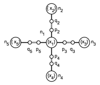
In Figure 3, node attributes are variables ranging over \mathbb{N}. The introduction of variables as attributes allows one to model node neighborhood-sensitive dynamics at the rewriting rule level as it will be illustrated in Section 5.
Refer to caption
Figure 3: Example of a pregraph H𝐻H such that: 𝒜H={{x1,x2,x3,x4,x5},+,×,=?=}{\cal A}_{H}=\{\mathbb{N}\cup\{x_{1},x_{2},x_{3},x_{4},x_{5}\},+,\times,=?=\}, 𝒩H={n1,n2,n3,n4,n5}subscript𝒩𝐻subscript𝑛1subscript𝑛2subscript𝑛3subscript𝑛4subscript𝑛5{\cal N}_{H}=\{n_{1},n_{2},n_{3},n_{4},n_{5}\}, 𝒫H={p2,p3,p4,p5,q2,q3,q4,q5}subscript𝒫𝐻subscript𝑝2subscript𝑝3subscript𝑝4subscript𝑝5subscript𝑞2subscript𝑞3subscript𝑞4subscript𝑞5{\cal P}_{H}=\{p_{2},p_{3},p_{4},p_{5},q_{2},q_{3},q_{4},q_{5}\}, 𝒫𝒩H={(p2,n1),(p3,n1),(p4,n1),(p5,n1),(q2,n2),(q3,n3),(q4,n4),(q5,n5)}𝒫subscript𝒩𝐻subscript𝑝2subscript𝑛1subscript𝑝3subscript𝑛1subscript𝑝4subscript𝑛1subscript𝑝5subscript𝑛1subscript𝑞2subscript𝑛2subscript𝑞3subscript𝑛3subscript𝑞4subscript𝑛4subscript𝑞5subscript𝑛5{\cal PN}_{H}=\{(p_{2},n_{1}),(p_{3},n_{1}),(p_{4},n_{1}),(p_{5},n_{1}),(q_{2},n_{2}),(q_{3},n_{3}),(q_{4},n_{4}),(q_{5},n_{5})\}, 𝒫𝒫H𝒫subscript𝒫𝐻{\cal PP}_{H} reduced to its non symmetric port-port connection is 𝒫𝒫H={(p2,q2),(p3,q3),(p4,q4),(p5,q5)}𝒫subscript𝒫𝐻subscript𝑝2subscript𝑞2subscript𝑝3subscript𝑞3subscript𝑝4subscript𝑞4subscript𝑝5subscript𝑞5{\cal PP}_{H}=\{(p_{2},q_{2}),(p_{3},q_{3}),(p_{4},q_{4}),(p_{5},q_{5})\}. λH(ni)={xi}subscript𝜆𝐻subscript𝑛𝑖subscript𝑥𝑖{\lambda_{H}}(n_{i})=\{x_{i}\} for i{1,2,3,4,5}𝑖12345i\in\{1,2,3,4,5\}, λH(pj)=λH(qj)=subscript𝜆𝐻subscript𝑝𝑗subscript𝜆𝐻subscript𝑞𝑗{\lambda_{H}}(p_{j})={\lambda_{H}}(q_{j})=\emptyset, for j{2,3,4,5}𝑗2345j\in\{2,3,4,5\}.

Below we introduce the definition of graphs used in this paper. In order to encode classical graph edges between nodes, restrictions over port associations are introduced. Intuitively, an edge e𝑒e between two nodes n1subscript𝑛1n_{1} and n2subscript𝑛2n_{2} will be encoded as two semi-edges (n1,p1)subscript𝑛1subscript𝑝1(n_{1},p_{1}) and (n2,p2)subscript𝑛2subscript𝑝2(n_{2},p_{2}) with p1subscript𝑝1p_{1} and p2subscript𝑝2p_{2} being ports which are linked via an association (p1,p2)subscript𝑝1subscript𝑝2(p_{1},p_{2}).

Definition 2 (Graph).

A graph, G𝐺G, is a pregraph G=(𝒩,𝒫,𝒫𝒩,𝒫𝒫,𝒜,λ)𝐺𝒩𝒫𝒫𝒩𝒫𝒫𝒜𝜆G=({\cal N},{\cal P},{\cal PN},{\cal PP},{\cal A},\lambda) such that :

  • (i)

    𝒫𝒩𝒫𝒩{\cal PN} is a relation 𝒫×𝒩absent𝒫𝒩\subseteq{\cal P}\times{\cal N} which associates at most one node to every port111The relation 𝒫𝒩𝒫𝒩{\cal PN} could be seen as a partial function 𝒫𝒩:𝒫𝒩:𝒫𝒩𝒫𝒩{\cal PN}:{\cal P}\rightarrow{\cal N} which associates to a given port p𝑝p, a node n𝑛n, 𝒫𝒩(p)=n𝒫𝒩𝑝𝑛{\cal PN}(p)=n ; thus building a semi-edge “port-node”.. That is to say, p𝒫,n1,n2𝒩,((p,n1)𝒫𝒩and(p,n2)𝒫𝒩)n1=n2formulae-sequencefor-all𝑝𝒫for-allsubscript𝑛1formulae-sequencesubscript𝑛2𝒩𝑝subscript𝑛1𝒫𝒩𝑎𝑛𝑑𝑝subscript𝑛2𝒫𝒩subscript𝑛1subscript𝑛2\forall p\in{\cal P},\forall n_{1},n_{2}\in{\cal N},((p,n_{1})\in{\cal PN}\;and\;(p,n_{2})\in{\cal PN})\implies n_{1}=n_{2}.

  • (ii)

    𝒫𝒫𝒫𝒫{\cal PP} is a symmetric binary relation222The relation 𝒫𝒫𝒫𝒫{\cal PP} could also be seen as an injective (partial) function from ports to ports such that p𝒫,𝒫𝒫(p)pformulae-sequencefor-all𝑝𝒫𝒫𝒫𝑝𝑝\forall p\in{\cal P},{\cal PP}(p)\neq p and p1,p2𝒫,𝒫𝒫(p1)=p2formulae-sequencefor-allsubscript𝑝1subscript𝑝2𝒫𝒫𝒫subscript𝑝1subscript𝑝2\forall p_{1},p_{2}\in{\cal P},{\cal PP}(p_{1})=p_{2} iff 𝒫𝒫(p2)=p1𝒫𝒫subscript𝑝2subscript𝑝1{\cal PP}(p_{2})=p_{1}. on ports, 𝒫𝒫𝒫×𝒫𝒫𝒫𝒫𝒫{\cal PP}\subseteq{\cal P}\times{\cal P}, such that p1,p2,p3𝒫,((p1,p2)𝒫𝒫\forall p_{1},p_{2},p_{3}\in{\cal P},((p_{1},p_{2})\in{\cal PP} and (p1,p3)𝒫𝒫)p2=p3(p_{1},p_{3})\in{\cal PP})\implies p_{2}=p_{3} and p𝒫,(p,p)𝒫𝒫formulae-sequencefor-all𝑝𝒫𝑝𝑝𝒫𝒫\forall p\in{\cal P},(p,p)\not\in{\cal PP}.

The main idea of our proposal is based on the use of equivalence relations over nodes and ports (merging certain nodes and ports under some conditions) in order to perform parallel graph rewriting in presence of overlapping rules. Thus, to a given pregraph H𝐻H, we associate two equivalence relations on ports, Psuperscript𝑃\equiv^{P}, and on nodes, Nsuperscript𝑁\equiv^{N}, as defined below.

Definition 3 (Psuperscript𝑃\equiv^{P}, Nsuperscript𝑁\equiv^{N}).

Let H=(𝒩H,𝒫H,𝒫𝒩H,𝒫𝒫H,𝒜H,λH)𝐻subscript𝒩𝐻subscript𝒫𝐻𝒫subscript𝒩𝐻𝒫subscript𝒫𝐻subscript𝒜𝐻subscript𝜆𝐻H=({\cal N}_{H},{\cal P}_{H},{\cal PN}_{H},{\cal PP}_{H},{\cal A}_{H},\lambda_{H}) be a pregraph. We define two relations Psuperscript𝑃\equiv^{P} and Nsuperscript𝑁\equiv^{N} respectively on ports (𝒫Hsubscript𝒫𝐻{\cal P}_{H}) and nodes (𝒩Hsubscript𝒩𝐻{\cal N}_{H}) of H𝐻H as follows:

  • Psuperscript𝑃\equiv^{P} is defined as (𝒫𝒫H𝒫𝒫H)superscript𝒫subscript𝒫𝐻𝒫subscript𝒫𝐻({\cal PP}_{H}\bullet{\cal PP}_{H})^{*}

  • Nsuperscript𝑁\equiv^{N} is defined as (𝒫𝒩HP𝒫𝒩)({\cal PN}_{H}^{-}\bullet\equiv^{P}\bullet{\cal PN})^{*}

where \bullet denotes relation composition, - the converse of a relation and the reflexive-transitive closure of a relation. We write [n]delimited-[]𝑛[n] (respectively, [p]delimited-[]𝑝[p]) the equivalence class of node n𝑛n (respectively, port p𝑝p).

Roughly speaking, relation Psuperscript𝑃\equiv^{P} is the closure of the first part of condition (ii) in Definition 2. The base case says that if two ports p1subscript𝑝1p_{1} and p2subscript𝑝2p_{2} are linked to a same port p𝑝p, then p1subscript𝑝1p_{1} and p2subscript𝑝2p_{2} are considered to be equivalent. Nsuperscript𝑁\equiv^{N} is almost the closure of condition (i) in Definition 2. That is, two nodes n1subscript𝑛1n_{1} and n2subscript𝑛2n_{2}, which are associated to a same port (or two equivalent ports), are considered as equivalent nodes.

Proposition 1.

Let H=(𝒩H,𝒫H,𝒫𝒩H,𝒫𝒫H,𝒜H,λH)𝐻subscript𝒩𝐻subscript𝒫𝐻𝒫subscript𝒩𝐻𝒫subscript𝒫𝐻subscript𝒜𝐻subscript𝜆𝐻H=({\cal N}_{H},{\cal P}_{H},{\cal PN}_{H},{\cal PP}_{H},{\cal A}_{H},\lambda_{H}) be a pregraph. The relations Psuperscript𝑃\equiv^{P} and Nsuperscript𝑁\equiv^{N} are equivalence relations.

Proof.

The reflexivity and transitivity of Psuperscript𝑃\equiv^{P} and Nsuperscript𝑁\equiv^{N} follow directly from their respective definitions. The symmetry of 𝒫𝒫H𝒫subscript𝒫𝐻{\cal PP}_{H} implies directly the symmetry of Psuperscript𝑃\equiv^{P} and Nsuperscript𝑁\equiv^{N}.

Remark 1.

The relations Psuperscript𝑃\equiv^{P} and Nsuperscript𝑁\equiv^{N} can be computed incrementally as follows:

Base cases: 0P={(x,x)x𝒫H}\equiv^{P}_{0}=\{(x,x)\mid x\in{\cal P}_{H}\} and   0N={(x,x)x𝒩H}\equiv^{N}_{0}=\{(x,x)\mid x\in{\cal N}_{H}\}

Inductive steps:

Rule I: if q,q𝒫H𝑞superscript𝑞subscript𝒫𝐻q,q^{\prime}\in{\cal P}_{H} such that, qiPqsubscriptsuperscript𝑃𝑖𝑞superscript𝑞q\equiv^{P}_{i}q^{\prime}, (q,p1)𝒫𝒫H𝑞subscript𝑝1𝒫subscript𝒫𝐻(q,p_{1})\in{\cal PP}_{H} and (q,p2)𝒫𝒫Hsuperscript𝑞subscript𝑝2𝒫subscript𝒫𝐻(q^{\prime},p_{2})\in{\cal PP}_{H} then p1i+1Pp2subscriptsuperscript𝑃𝑖1subscript𝑝1subscript𝑝2p_{1}\equiv^{P}_{i+1}p_{2}.
Rule II: if p1𝒫Hsubscript𝑝1subscript𝒫𝐻p_{1}\in{\cal P}_{H}, p2𝒫Hsubscript𝑝2subscript𝒫𝐻p_{2}\in{\cal P}_{H}, (p1,n1)𝒫𝒩Hsubscript𝑝1subscript𝑛1𝒫subscript𝒩𝐻(p_{1},n_{1})\in{\cal PN}_{H}, (p2,n2)𝒫𝒩Hsubscript𝑝2subscript𝑛2𝒫subscript𝒩𝐻(p_{2},n_{2})\in{\cal PN}_{H} and p1iPp2subscriptsuperscript𝑃𝑖subscript𝑝1subscript𝑝2p_{1}\equiv^{P}_{i}p_{2} then n1i+1Nn2subscriptsuperscript𝑁𝑖1subscript𝑛1subscript𝑛2n_{1}\equiv^{N}_{i+1}n_{2}.
Rule III: If n1iNnsubscriptsuperscript𝑁𝑖subscript𝑛1superscript𝑛n_{1}\equiv^{N}_{i}n^{\prime} and niNn2subscriptsuperscript𝑁𝑖superscript𝑛subscript𝑛2n^{\prime}\equiv^{N}_{i}n_{2} then n1i+1Nn2subscriptsuperscript𝑁𝑖1subscript𝑛1subscript𝑛2n_{1}\equiv^{N}_{i+1}n_{2}.

Proposition 2.

The limit of the series (iP)i0subscriptsuperscriptsubscript𝑖𝑃𝑖0(\equiv_{i}^{P})_{i\geq 0} is Psuperscript𝑃\equiv^{P}.

Proof.

Since the set of ports is finite then the limit of the series is reached within a finite number of steps.

\Rightarrow : Let p1,p2𝒫Hsubscript𝑝1subscript𝑝2subscript𝒫𝐻p_{1},p_{2}\in{\cal P}_{H}, such that p1kPp2superscriptsubscript𝑘𝑃subscript𝑝1subscript𝑝2p_{1}\equiv_{k}^{P}p_{2} for some k𝑘k, let us prove by induction on k𝑘k, that (p1,p2)(𝒫𝒫𝒫𝒫)ksubscript𝑝1subscript𝑝2superscript𝒫𝒫𝒫𝒫𝑘(p_{1},p_{2})\in({\cal PP}\bullet{\cal PP})^{k}.

  • case k=0𝑘0k=0 : p10Pp2superscriptsubscript0𝑃subscript𝑝1subscript𝑝2p_{1}\equiv_{0}^{P}p_{2} thus p1=p2subscript𝑝1subscript𝑝2p_{1}=p_{2} and (p1,p2)(𝒫𝒫𝒫𝒫)0subscript𝑝1subscript𝑝2superscript𝒫𝒫𝒫𝒫0(p_{1},p_{2})\in({\cal PP}\bullet{\cal PP})^{0}.

  • Induction step, case k=k+1𝑘superscript𝑘1k=k^{\prime}+1 : Let us assume p1k+1Pp2superscriptsubscriptsuperscript𝑘1𝑃subscript𝑝1subscript𝑝2p_{1}\equiv_{k^{\prime}+1}^{P}p_{2}. In this case, from rule I, there exist q,q𝒫H𝑞superscript𝑞subscript𝒫𝐻q,q^{\prime}\in{\cal P}_{H} such that, qkPqsubscriptsuperscript𝑃superscript𝑘𝑞superscript𝑞q\equiv^{P}_{k^{\prime}}q^{\prime}, (q,p1)𝒫𝒫H𝑞subscript𝑝1𝒫subscript𝒫𝐻(q,p_{1})\in{\cal PP}_{H} and (q,p2)𝒫𝒫Hsuperscript𝑞subscript𝑝2𝒫subscript𝒫𝐻(q^{\prime},p_{2})\in{\cal PP}_{H}. qkPqsubscriptsuperscript𝑃superscript𝑘𝑞superscript𝑞q\equiv^{P}_{k^{\prime}}q^{\prime} implies by induction hypothesis that (q,q)(𝒫𝒫𝒫𝒫)k𝑞superscript𝑞superscript𝒫𝒫𝒫𝒫superscript𝑘(q,q^{\prime})\in({\cal PP}\bullet{\cal PP})^{k^{\prime}}. Thus (p1,p2)(𝒫𝒫𝒫𝒫)k+1subscript𝑝1subscript𝑝2superscript𝒫𝒫𝒫𝒫superscript𝑘1(p_{1},p_{2})\in({\cal PP}\bullet{\cal PP})^{k^{\prime}+1}.

  • Therefore for all k𝑘k, p1kPp2superscriptsubscript𝑘𝑃subscript𝑝1subscript𝑝2p_{1}\equiv_{k}^{P}p_{2} implies (p1,p2)(𝒫𝒫𝒫𝒫)ksubscript𝑝1subscript𝑝2superscript𝒫𝒫𝒫𝒫𝑘(p_{1},p_{2})\in({\cal PP}\bullet{\cal PP})^{k}, and thus, p1Pp2superscript𝑃subscript𝑝1subscript𝑝2p_{1}\equiv^{P}p_{2}.

\Leftarrow Let p1Pp2superscript𝑃subscript𝑝1subscript𝑝2p_{1}\equiv^{P}p_{2}. By definition of Psuperscript𝑃\equiv^{P}, there exists a natural number k𝑘k such that (p1,p2)(𝒫𝒫𝒫𝒫)ksubscript𝑝1subscript𝑝2superscript𝒫𝒫𝒫𝒫𝑘(p_{1},p_{2})\in({\cal PP}\bullet{\cal PP})^{k}. It is then straightforward that p1kPp2superscriptsubscript𝑘𝑃subscript𝑝1subscript𝑝2p_{1}\equiv_{k}^{P}p_{2}. ∎

Likewise, we can easily show the following proposition regarding relation Nsuperscript𝑁\equiv^{N}.

Proposition 3.

The limit of the series (iN)i0subscriptsuperscriptsubscript𝑖𝑁𝑖0(\equiv_{i}^{N})_{i\geq 0} is Nsuperscript𝑁\equiv^{N}.

Proof.

Since the sets of nodes and ports are finite then the limit of the series is reached within a finite number of steps. \Rightarrow : Let n1,n2𝒩Hsubscript𝑛1subscript𝑛2subscript𝒩𝐻n_{1},n_{2}\in{\cal N}_{H}, such that n1kNn2superscriptsubscript𝑘𝑁subscript𝑛1subscript𝑛2n_{1}\equiv_{k}^{N}n_{2} for some k𝑘k , let us prove by induction on k𝑘k, that (n1,n2)Nsubscript𝑛1subscript𝑛2superscript𝑁(n_{1},n_{2})\in\equiv^{N}.

  • case k=0𝑘0k=0 : obvious.

  • Induction step, case k=k+1𝑘superscript𝑘1k=k^{\prime}+1 : Let us assume n1k+1Nn2superscriptsubscriptsuperscript𝑘1𝑁subscript𝑛1subscript𝑛2n_{1}\equiv_{k^{\prime}+1}^{N}n_{2}. We distinguish two sub-cases according to the used rules, i.e. Rule II or Rule III.

    • Rule III.

      According to Rule III, there exists a node nsuperscript𝑛n^{\prime} such that n1kNnsuperscriptsubscriptsuperscript𝑘𝑁subscript𝑛1superscript𝑛n_{1}\equiv_{k^{\prime}}^{N}n^{\prime} and nkNn2superscriptsubscriptsuperscript𝑘𝑁superscript𝑛subscript𝑛2n^{\prime}\equiv_{k^{\prime}}^{N}n_{2}. From the induction hypothesis, we have n1kNnn1Nnsuperscriptsubscriptsuperscript𝑘𝑁subscript𝑛1superscript𝑛subscript𝑛1superscript𝑁superscript𝑛n_{1}\equiv_{k^{\prime}}^{N}n^{\prime}\implies n_{1}\equiv^{N}n^{\prime} and nkNn2nNn2superscriptsubscriptsuperscript𝑘𝑁superscript𝑛subscript𝑛2superscript𝑛superscript𝑁subscript𝑛2n^{\prime}\equiv_{k^{\prime}}^{N}n_{2}\implies n^{\prime}\equiv^{N}n_{2}. Then by transitivity of Nsuperscript𝑁\equiv^{N} we have n1Nn2superscript𝑁subscript𝑛1subscript𝑛2n_{1}\equiv^{N}n_{2}.

    • Rule II.

      According to Rule II, there exist two ports p1subscript𝑝1p_{1} and p2subscript𝑝2p_{2} in 𝒫Hsubscript𝒫𝐻{\cal P}_{H} such that (p1,n1)𝒫𝒩Hsubscript𝑝1subscript𝑛1𝒫subscript𝒩𝐻(p_{1},n_{1})\in{\cal PN}_{H}, (p2,n2)𝒫𝒩Hsubscript𝑝2subscript𝑛2𝒫subscript𝒩𝐻(p_{2},n_{2})\in{\cal PN}_{H} and p1kPp2subscriptsuperscript𝑃superscript𝑘subscript𝑝1subscript𝑝2p_{1}\equiv^{P}_{k^{\prime}}p_{2}. From Proposition 2, p1kPp2p1Pp2subscriptsuperscript𝑃superscript𝑘subscript𝑝1subscript𝑝2subscript𝑝1superscript𝑃subscript𝑝2p_{1}\equiv^{P}_{k^{\prime}}p_{2}\implies p_{1}\equiv^{P}p_{2}, and thus, there exists an index i𝑖i such that (p1,p2)(𝒫𝒫H𝒫𝒫H)isubscript𝑝1subscript𝑝2superscript𝒫subscript𝒫𝐻𝒫subscript𝒫𝐻𝑖(p_{1},p_{2})\in({\cal PP}_{H}\bullet{\cal PP}_{H})^{i}. Since (p1,n1)𝒫𝒩Hsubscript𝑝1subscript𝑛1𝒫subscript𝒩𝐻(p_{1},n_{1})\in{\cal PN}_{H} and (p2,n2)𝒫𝒩Hsubscript𝑝2subscript𝑛2𝒫subscript𝒩𝐻(p_{2},n_{2})\in{\cal PN}_{H} we conclude that (n1,n2)(𝒫𝒩HP𝒫𝒩H)(n_{1},n_{2})\in({\cal PN}_{H}^{-}\bullet\equiv^{P}\bullet{\cal PN}_{H})

\Leftarrow Let n1Nn2superscript𝑁subscript𝑛1subscript𝑛2n_{1}\equiv^{N}n_{2}. Then by definition of Nsuperscript𝑁\equiv^{N} there exists a natural number k𝑘k such that (n1,n2)(𝒫𝒩HP𝒫𝒩H)k(n_{1},n_{2})\in({\cal PN}_{H}^{-}\bullet\equiv^{P}\bullet{\cal PN}_{H})^{k}. This means that there is a chain of connections consisting of tuples of the form (mi,pi).piPpi.(pi,mi+1)formulae-sequencesubscript𝑚𝑖subscript𝑝𝑖superscript𝑃subscript𝑝𝑖subscriptsuperscript𝑝𝑖subscriptsuperscript𝑝𝑖subscript𝑚𝑖1(m_{i},p_{i}).p_{i}\equiv^{P}p^{\prime}_{i}.(p^{\prime}_{i},m_{i+1}) for i{0,,k}𝑖0𝑘i\in\{0,...,k\} such that m0=n1subscript𝑚0subscript𝑛1m_{0}=n_{1} and mk=n2subscript𝑚𝑘subscript𝑛2m_{k}=n_{2}. From rule III, it is easy to deduce the existence of ksuperscript𝑘k^{\prime}, such that n1kNn2subscriptsuperscript𝑁superscript𝑘subscript𝑛1subscript𝑛2n_{1}\equiv^{N}_{k^{\prime}}n_{2}.

The equivalence relations Psuperscript𝑃\equiv^{P} and Nsuperscript𝑁\equiv^{N} are used to introduce the notion of quotient pregraph as defined below.

Definition 4 (Quotient Pregraph).

Let H=(𝒩H,𝒫H,𝒫𝒩H,𝒫𝒫H,𝒜H,λH)𝐻subscript𝒩𝐻subscript𝒫𝐻𝒫subscript𝒩𝐻𝒫subscript𝒫𝐻subscript𝒜𝐻subscript𝜆𝐻H=({\cal N}_{H},{\cal P}_{H},{\cal PN}_{H},{\cal PP}_{H},{\cal A}_{H},\lambda_{H}) be a pregraph and Psuperscript𝑃\equiv^{P} and Nsuperscript𝑁\equiv^{N} two equivalence relations over ports and nodes respectively. We write H¯¯𝐻\overline{H} the pregraph  H¯=(𝒩H¯,𝒫H¯,𝒫𝒩H¯,𝒫𝒫H¯,𝒜H¯,λH¯)¯𝐻subscript𝒩¯𝐻subscript𝒫¯𝐻𝒫subscript𝒩¯𝐻𝒫subscript𝒫¯𝐻subscript𝒜¯𝐻subscript𝜆¯𝐻\overline{H}=({\cal N}_{\overline{H}},{\cal P}_{\overline{H}},{\cal PN}_{\overline{H}},{\cal PP}_{\overline{H}},{\cal A}_{\overline{H}},\lambda_{\overline{H}}) where 𝒩H¯={[n]|n𝒩H}subscript𝒩¯𝐻conditional-setdelimited-[]𝑛𝑛subscript𝒩𝐻{\cal N}_{\overline{H}}=\{[n]\;|\;n\in{\cal N}_{H}\}, 𝒫H¯={[p]|p𝒫H}subscript𝒫¯𝐻conditional-setdelimited-[]𝑝𝑝subscript𝒫𝐻{\cal P}_{\overline{H}}=\{[p]\;|\;p\in{\cal P}_{H}\}, 𝒫𝒩H¯={([p],[n])|(p,n)𝒫𝒩H}𝒫subscript𝒩¯𝐻conditional-setdelimited-[]𝑝delimited-[]𝑛𝑝𝑛𝒫subscript𝒩𝐻{\cal PN}_{\overline{H}}=\{([p],[n])\;|\;(p,n)\in{\cal PN}_{H}\}, 𝒫𝒫H¯={([p],[q])|(p,q)𝒫𝒫H}𝒫subscript𝒫¯𝐻conditional-setdelimited-[]𝑝delimited-[]𝑞𝑝𝑞𝒫subscript𝒫𝐻{\cal PP}_{\overline{H}}=\{([p],[q])\;|\;(p,q)\in{\cal PP}_{H}\}, 𝒜H¯=𝒜Hsubscript𝒜¯𝐻subscript𝒜𝐻{\cal A}_{\overline{H}}={\cal A}_{H} and λH¯([x])=x[x]λH(x)subscript𝜆¯𝐻delimited-[]𝑥subscriptsuperscript𝑥delimited-[]𝑥subscript𝜆𝐻superscript𝑥\lambda_{\overline{H}}([x])=\cup_{x^{\prime}\in[x]}\lambda_{H}(x^{\prime}) where [x]𝒩H¯𝒫H¯delimited-[]𝑥subscript𝒩¯𝐻subscript𝒫¯𝐻{[x]}\in{\cal N}_{\overline{H}}\uplus{\cal P}_{\overline{H}}

Example 2.

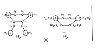
Let H=(𝒩H,𝒫H,𝒫𝒩H,𝒫𝒫H,𝒜H,λH)𝐻subscript𝒩𝐻subscript𝒫𝐻𝒫subscript𝒩𝐻𝒫subscript𝒫𝐻subscript𝒜𝐻subscript𝜆𝐻H=({\cal N}_{H},{\cal P}_{H},{\cal PN}_{H},{\cal PP}_{H},{\cal A}_{H},\lambda_{H}) be a pregraph as depicted on the left of Figure 4, with 𝒩H={n1,n2,n3,n4}subscript𝒩𝐻subscript𝑛1subscript𝑛2subscript𝑛3subscript𝑛4{\cal N}_{H}=\{n_{1},n_{2},n_{3},n_{4}\}, 𝒫H={p1,p2,p3,p4,p5,p6}subscript𝒫𝐻subscript𝑝1subscript𝑝2subscript𝑝3subscript𝑝4subscript𝑝5subscript𝑝6{\cal P}_{H}=\{p_{1},p_{2},p_{3},p_{4},p_{5},p_{6}\}, 𝒫𝒩H={(p1,n1),(p5,n1),{\cal PN}_{H}=\{(p_{1},n_{1}),(p_{5},n_{1}), (p2,n2),(p6,n2),(p4,n3),(p3,n4)}(p_{2},n_{2}),(p_{6},n_{2}),(p_{4},n_{3}),(p_{3},n_{4})\}, 𝒫𝒫H={(p1,p2),(p1,p4),(p2,p3),(p3,p4),(p5,p6)}𝒫subscript𝒫𝐻subscript𝑝1subscript𝑝2subscript𝑝1subscript𝑝4subscript𝑝2subscript𝑝3subscript𝑝3subscript𝑝4subscript𝑝5subscript𝑝6{\cal PP}_{H}=\{(p_{1},p_{2}),(p_{1},p_{4}),(p_{2},p_{3}),(p_{3},p_{4}),(p_{5},p_{6})\},
𝒜H=subscript𝒜𝐻{\cal A}_{H}=\mathbb{N}, λ𝒩H(n1)=λ𝒩H(n4)={1}subscript𝜆subscript𝒩𝐻subscript𝑛1subscript𝜆subscript𝒩𝐻subscript𝑛41\lambda_{{\cal N}_{H}}(n_{1})=\lambda_{{\cal N}_{H}}(n_{4})=\{1\}, λ𝒩H(n2)=λ𝒩H(n3)={2}subscript𝜆subscript𝒩𝐻subscript𝑛2subscript𝜆subscript𝒩𝐻subscript𝑛32\lambda_{{\cal N}_{H}}(n_{2})=\lambda_{{\cal N}_{H}}(n_{3})=\{2\}, i{1,,6},λ𝒫H(pi)=formulae-sequencefor-all𝑖16subscript𝜆subscript𝒫𝐻subscript𝑝𝑖\forall i\in\{1,...,6\},\lambda_{{\cal P}_{H}}(p_{i})=\emptyset,

We obtain H¯=(𝒩H¯,𝒫H¯,𝒫𝒩H¯,𝒫𝒫H¯,𝒜H¯,λH¯)¯𝐻subscript𝒩¯𝐻subscript𝒫¯𝐻𝒫subscript𝒩¯𝐻𝒫subscript𝒫¯𝐻subscript𝒜¯𝐻subscript𝜆¯𝐻\overline{H}=({\cal N}_{\overline{H}},{\cal P}_{\overline{H}},{\cal PN}_{\overline{H}},{\cal PP}_{\overline{H}},{\cal A}_{\overline{H}},\lambda_{\overline{H}}), as depicted on the right of Figure 4, with

  • 𝒩H¯={[n1],[n2]}subscript𝒩¯𝐻delimited-[]subscript𝑛1delimited-[]subscript𝑛2{\cal N}_{\overline{H}}=\{[n_{1}],[n_{2}]\} with [n1]={n1,n4}delimited-[]subscript𝑛1subscript𝑛1subscript𝑛4[n_{1}]=\{n_{1},n_{4}\}, [n2]={n2,n3}delimited-[]subscript𝑛2subscript𝑛2subscript𝑛3[n_{2}]=\{n_{2},n_{3}\},

  • 𝒫H¯={[p1],[p2],[p5],[p6]}subscript𝒫¯𝐻delimited-[]subscript𝑝1delimited-[]subscript𝑝2delimited-[]subscript𝑝5delimited-[]subscript𝑝6{\cal P}_{\overline{H}}=\{[p_{1}],[p_{2}],[p_{5}],[p_{6}]\} with [p1]={p1,p3}delimited-[]subscript𝑝1subscript𝑝1subscript𝑝3[p_{1}]=\{p_{1},p_{3}\}, [p2]={p2,p4}delimited-[]subscript𝑝2subscript𝑝2subscript𝑝4[p_{2}]=\{p_{2},p_{4}\}, [p5]={p5}delimited-[]subscript𝑝5subscript𝑝5[p_{5}]=\{p_{5}\}, [p6]={p6}delimited-[]subscript𝑝6subscript𝑝6[p_{6}]=\{p_{6}\},

  • 𝒫𝒩H¯={([p1],[n1]),([p5],[n1]),([p2],[n2]),([p6],[n2])}𝒫subscript𝒩¯𝐻delimited-[]subscript𝑝1delimited-[]subscript𝑛1delimited-[]subscript𝑝5delimited-[]subscript𝑛1delimited-[]subscript𝑝2delimited-[]subscript𝑛2delimited-[]subscript𝑝6delimited-[]subscript𝑛2{\cal PN}_{\overline{H}}=\{([p_{1}],[n_{1}]),([p_{5}],[n_{1}]),([p_{2}],[n_{2}]),([p_{6}],[n_{2}])\},

  • 𝒫𝒫H¯={([p1],[p2]),([p5],[p6])}𝒫subscript𝒫¯𝐻delimited-[]subscript𝑝1delimited-[]subscript𝑝2delimited-[]subscript𝑝5delimited-[]subscript𝑝6{\cal PP}_{\overline{H}}=\{([p_{1}],[p_{2}]),([p_{5}],[p_{6}])\},

  • 𝒜H¯=𝒜Hsubscript𝒜¯𝐻subscript𝒜𝐻{\cal A}_{\overline{H}}={\cal A}_{H}

  • λ𝒩H¯([n1])={1}subscript𝜆subscript𝒩¯𝐻delimited-[]subscript𝑛11\lambda_{{\cal N}_{\overline{H}}}([n_{1}])=\{1\}, λ𝒩H¯([n2])={2}subscript𝜆subscript𝒩¯𝐻delimited-[]subscript𝑛22\lambda_{{\cal N}_{\overline{H}}}([n_{2}])=\{2\}, λ𝒫H¯([p1])=λ𝒫H¯([p2])=λ𝒫H¯([p5])=λ𝒫H¯([p6])=subscript𝜆subscript𝒫¯𝐻delimited-[]subscript𝑝1subscript𝜆subscript𝒫¯𝐻delimited-[]subscript𝑝2subscript𝜆subscript𝒫¯𝐻delimited-[]subscript𝑝5subscript𝜆subscript𝒫¯𝐻delimited-[]subscript𝑝6\lambda_{{\cal P}_{\overline{H}}}([p_{1}])=\lambda_{{\cal P}_{\overline{H}}}([p_{2}])=\lambda_{{\cal P}_{\overline{H}}}([p_{5}])=\lambda_{{\cal P}_{\overline{H}}}([p_{6}])=\emptyset.

Refer to caption
Refer to caption
Figure 4: (a) A pregraph H𝐻H (b) and its corresponding quotient pregraph H¯¯𝐻\overline{H}.
Example 3.

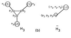
Figure 5 illustrates two computations of quotient pregraphs.

Remark 2.

If H𝐻H is a graph, H¯¯𝐻\overline{H} and H𝐻H are isomorphic. Indeed, in a graph, a port can be associated (resp. linked) to at most one node (resp. one port).

The following definition introduces some vocabulary and notations.

Definition 5 (Path, Loop).
  • A path πH(p1,pk)subscript𝜋𝐻subscript𝑝1subscript𝑝𝑘\pi_{H}(p_{1},p_{k}) between two (possibly the same) nodes p1subscript𝑝1p_{1} and pksubscript𝑝𝑘p_{k} in a pregraph H𝐻H is a sequence of ports of H𝐻H written πH(p1,pk)=(p1,p2,,pk)subscript𝜋𝐻subscript𝑝1subscript𝑝𝑘subscript𝑝1subscript𝑝2subscript𝑝𝑘\pi_{H}(p_{1},p_{k})=(p_{1},p_{2},\ldots,p_{k}) such that {(pi,pi+1)|i=1,2,,k1}𝒫𝒫Hconditional-setsubscript𝑝𝑖subscript𝑝𝑖1𝑖12𝑘1𝒫subscript𝒫𝐻\{(p_{i},p_{i+1})\;|\;i=1,2,\ldots,k-1\}\subseteq{\cal PP}_{H} and k𝑘k\in\mathbb{N} with k>0𝑘0k>0.

  • The length of a path πH(p1,pk)=(p1,p2,,pk)subscript𝜋𝐻subscript𝑝1subscript𝑝𝑘subscript𝑝1subscript𝑝2subscript𝑝𝑘\pi_{H}(p_{1},p_{k})=(p_{1},p_{2},\ldots,p_{k}) is (πH(p1,pk))=k1subscript𝜋𝐻subscript𝑝1subscript𝑝𝑘𝑘1\sharp({\pi_{H}}(p_{1},p_{k}))=k-1.

  • An even path (resp. odd path) is a path such that its length is even (resp. odd).

  • A loop is a closed path, i.e., a path πH=(p1,p2,,pk)subscript𝜋𝐻subscript𝑝1subscript𝑝2subscript𝑝𝑘\pi_{H}=(p_{1},p_{2},\ldots,p_{k}) such that p1=pksubscript𝑝1subscript𝑝𝑘p_{1}=p_{k}. An even loop (resp. odd loop) is an even closed path (resp. odd closed path).

From the definitions above, one can show the following statements.

Proposition 4.

Let H=(𝒩H,𝒫H,𝒫𝒩H,𝒫𝒫H,𝒜H,λH)𝐻subscript𝒩𝐻subscript𝒫𝐻𝒫subscript𝒩𝐻𝒫subscript𝒫𝐻subscript𝒜𝐻subscript𝜆𝐻H=({\cal N}_{H},{\cal P}_{H},{\cal PN}_{H},{\cal PP}_{H},{\cal A}_{H},\lambda_{H}) be a pregraph. Let q,q𝑞superscript𝑞q,q^{\prime} be two ports in 𝒫Hsubscript𝒫𝐻{\cal P}_{H}. qPqsuperscript𝑃𝑞superscript𝑞q\equiv^{P}q^{\prime} iff there exists an even path between q𝑞q and qsuperscript𝑞q^{\prime} in H𝐻H.

Proof.

If qPqsuperscript𝑃𝑞superscript𝑞q\equiv^{P}q^{\prime} then, by definition, (q,q)(𝒫𝒫H𝒫𝒫H)𝑞superscript𝑞superscript𝒫subscript𝒫𝐻𝒫subscript𝒫𝐻(q,q^{\prime})\in({\cal PP}_{H}\bullet{\cal PP}_{H})^{*} hence there exists an even path between q𝑞q and qsuperscript𝑞q^{\prime}. Conversely, if there exists an even path between q𝑞q and qsuperscript𝑞q^{\prime} in H𝐻H then (q,q)(𝒫𝒫H𝒫𝒫H)𝑞superscript𝑞superscript𝒫subscript𝒫𝐻𝒫subscript𝒫𝐻(q,q^{\prime})\in({\cal PP}_{H}\bullet{\cal PP}_{H})^{*} and thus qPqsuperscript𝑃𝑞superscript𝑞q\equiv^{P}q^{\prime}. ∎

Proposition 5.

Let H=(𝒩H,𝒫H,𝒫𝒩H,𝒫𝒫H,𝒜H,λH)𝐻subscript𝒩𝐻subscript𝒫𝐻𝒫subscript𝒩𝐻𝒫subscript𝒫𝐻subscript𝒜𝐻subscript𝜆𝐻H=({\cal N}_{H},{\cal P}_{H},{\cal PN}_{H},{\cal PP}_{H},{\cal A}_{H},\lambda_{H}) be a pregraph. H¯¯𝐻\overline{H} is a graph iff H𝐻H has no odd loop.

Proof.

Let H¯=(𝒩H¯,𝒫H¯,𝒫𝒩H¯,𝒫𝒫H¯,𝒜H¯,,λH¯)\overline{H}=({\cal N}_{\overline{H}},{\cal P}_{\overline{H}},{\cal PN}_{\overline{H}},{\cal PP}_{\overline{H}},{\cal A}_{\overline{H}},,\lambda_{\overline{H}}). The relations 𝒫𝒩H¯𝒫subscript𝒩¯𝐻{\cal PN}_{\overline{H}} and 𝒫𝒫H¯𝒫subscript𝒫¯𝐻{\cal PP}_{\overline{H}} are functional by construction. In order to show that H¯¯𝐻\overline{H} is indeed a graph, It remains to prove that 𝒫𝒫H¯𝒫subscript𝒫¯𝐻{\cal PP}_{\overline{H}} is not anti-reflexive iff there is an odd loop in H𝐻H.

  • \Rightarrow

    Assume that 𝒫𝒫H¯𝒫subscript𝒫¯𝐻{\cal PP}_{\overline{H}} is not anti-reflexive. Then, there exists q𝒫H𝑞subscript𝒫𝐻q\in{\cal P}_{H} such that ([q],[q])𝒫𝒫H¯delimited-[]𝑞delimited-[]𝑞𝒫subscript𝒫¯𝐻([q],[q])\in{\cal PP}_{\overline{H}}. Thus, either (q,q)𝒫𝒫H𝑞𝑞𝒫subscript𝒫𝐻(q,q)\in{\cal PP}_{H} which constitute an odd loop of length one or there exists a port qsuperscript𝑞q^{\prime}, different from q𝑞q, such that (q,q)𝒫𝒫H𝑞superscript𝑞𝒫subscript𝒫𝐻(q,q^{\prime})\in{\cal PP}_{H} and qPqsuperscript𝑃superscript𝑞𝑞q^{\prime}\equiv^{P}q. In this last case, from Proposition4, qPqsuperscript𝑃superscript𝑞𝑞q^{\prime}\equiv^{P}q implies the existence of an even path from qsuperscript𝑞q^{\prime} to q𝑞q. Then adding the link (q,q)𝑞superscript𝑞(q,q^{\prime}) to this path builds a loop from q𝑞q to q𝑞q in H𝐻H of odd length.

  • \Leftarrow

    Assume there is an odd loop containing a port q𝑞q in H𝐻H. Then either the loop is of the form (q,q)𝑞𝑞(q,q) and thus (q,q)𝒫𝒫H𝑞𝑞𝒫subscript𝒫𝐻(q,q)\in{\cal PP}_{H} and in this case ([q],[q])𝒫𝒫H¯delimited-[]𝑞delimited-[]𝑞𝒫subscript𝒫¯𝐻([q],[q])\in{\cal PP}_{\overline{H}}, or there exists a port qsuperscript𝑞q^{\prime} different from q𝑞q such that the loop is of the form (q,q,,q)𝑞superscript𝑞𝑞(q,q^{\prime},\ldots,q). In this last case, (q,q)𝒫𝒫H𝑞superscript𝑞𝒫subscript𝒫𝐻(q,q^{\prime})\in{\cal PP}_{H} and the path πH(q,q)subscript𝜋𝐻superscript𝑞𝑞\pi_{H}(q^{\prime},q) is even. Thus, [q]=[q]delimited-[]𝑞delimited-[]superscript𝑞[q]=[q^{\prime}] which implies that ([q],[q])𝒫𝒫H¯delimited-[]𝑞delimited-[]𝑞𝒫subscript𝒫¯𝐻([q],[q])\in{\cal PP}_{\overline{H}}.

Refer to caption
Refer to caption
Figure 5: (a) A pregraph H2subscript𝐻2H_{2} and its corresponding quotient pregraph H¯2subscript¯𝐻2\overline{H}_{2} which is a graph. (b) A pregraph H3subscript𝐻3H_{3} and its corresponding quotient pregraph H¯3subscript¯𝐻3\overline{H}_{3} which is not a graph.

Below, we define the notion of homomorphisms of pregraphs and graphs. This notion assumes the existence of homomorphisms over attributes [7].

Definition 6 (Pregraph and Graph Homomorphism).

Let l=(𝒩l,𝒫l,𝒫𝒩l,𝒫𝒫l,𝒜l,λl)𝑙subscript𝒩𝑙subscript𝒫𝑙𝒫subscript𝒩𝑙𝒫subscript𝒫𝑙subscript𝒜𝑙subscript𝜆𝑙l=({\cal N}_{l},{\cal P}_{l},{\cal PN}_{l},{\cal PP}_{l},{\cal A}_{l},\lambda_{l}) and g=(𝒩g,𝒫g,𝒫𝒩g,𝒫𝒫g,𝒜g,λg)𝑔subscript𝒩𝑔subscript𝒫𝑔𝒫subscript𝒩𝑔𝒫subscript𝒫𝑔subscript𝒜𝑔subscript𝜆𝑔g=({\cal N}_{g},{\cal P}_{g},{\cal PN}_{g},{\cal PP}_{g},{\cal A}_{g},\lambda_{g}) be two pregraphs. Let a:𝒜l𝒜g:𝑎subscript𝒜𝑙subscript𝒜𝑔a:{\cal A}_{l}\to{\cal A}_{g} be a homomorphism over attributes. A pregraph homomorphism, ha:lg:superscript𝑎𝑙𝑔h^{a}:l\rightarrow g, between l𝑙l and g𝑔g, built over attribute homomorphism a𝑎a, is defined by two functions hNa:𝒩l𝒩g:subscriptsuperscript𝑎𝑁subscript𝒩𝑙subscript𝒩𝑔h^{a}_{N}:{\cal N}_{l}\rightarrow{\cal N}_{g} and hPa:𝒫l𝒫g:subscriptsuperscript𝑎𝑃subscript𝒫𝑙subscript𝒫𝑔h^{a}_{P}:{\cal P}_{l}\rightarrow{\cal P}_{g} such that (i) (p1,n1)𝒫𝒩lfor-allsubscript𝑝1subscript𝑛1𝒫subscript𝒩𝑙\forall(p_{1},n_{1})\in{\cal PN}_{l}, (hPa(p1),hNa(n1))𝒫𝒩g,subscriptsuperscript𝑎𝑃subscript𝑝1subscriptsuperscript𝑎𝑁subscript𝑛1𝒫subscript𝒩𝑔(h^{a}_{P}(p_{1}),h^{a}_{N}(n_{1}))\in{\cal PN}_{g}, (ii) (p1,p2)𝒫𝒫lfor-allsubscript𝑝1subscript𝑝2𝒫subscript𝒫𝑙\forall(p_{1},p_{2})\in{\cal PP}_{l}, (hPa(p1),hPa(p2))𝒫𝒫gsubscriptsuperscript𝑎𝑃subscript𝑝1subscriptsuperscript𝑎𝑃subscript𝑝2𝒫subscript𝒫𝑔(h^{a}_{P}(p_{1}),h^{a}_{P}(p_{2}))\in{\cal PP}_{g}, (iii) n1𝒩l,a(λl(n1))λg(hNa(n1))formulae-sequencefor-allsubscript𝑛1subscript𝒩𝑙𝑎subscript𝜆𝑙subscript𝑛1subscript𝜆𝑔subscriptsuperscript𝑎𝑁subscript𝑛1\forall n_{1}\in{\cal N}_{l},a(\lambda_{l}(n_{1}))\subseteq\lambda_{g}(h^{a}_{N}(n_{1})) and (iv) p1𝒫l,a(λl(p1))λg(hPa(p1))formulae-sequencefor-allsubscript𝑝1subscript𝒫𝑙𝑎subscript𝜆𝑙subscript𝑝1subscript𝜆𝑔subscriptsuperscript𝑎𝑃subscript𝑝1\forall p_{1}\in{\cal P}_{l},a(\lambda_{l}(p_{1}))\subseteq\lambda_{g}(h^{a}_{P}(p_{1})).

A graph homomorphism is a pregraph homomorphism between two graphs.

Notation: Let E𝐸E be a set of attributes, we denote by a(E)𝑎𝐸a(E) the set a(E)={a(e)|eE}𝑎𝐸conditional-set𝑎𝑒𝑒𝐸a(E)=\{a(e)\;|\;e\in E\}.

Proposition 6.

Let H𝐻H and Hsuperscript𝐻H^{\prime} be two isomorphic pregraphs. Then H¯¯𝐻\overline{H} and H¯¯superscript𝐻\overline{H^{\prime}} are isomorphic.

Proof.

Let ha:HH:superscript𝑎𝐻superscript𝐻h^{a}:H\to H^{\prime} be a pregraph isomorphism. We define ha¯:H¯H¯:¯superscript𝑎¯𝐻superscript¯𝐻{\overline{h^{a}}}:\overline{H}\to\overline{H}^{\prime} as follows: for all ports p,p𝑝superscript𝑝p,p^{\prime} in H𝐻H, nodes n𝑛n in H, hNa¯([n])=[hNa(n)]¯subscriptsuperscript𝑎𝑁delimited-[]𝑛delimited-[]subscriptsuperscript𝑎𝑁𝑛{\overline{h^{a}_{N}}}([n])={[h^{a}_{N}(n)]}, hPa¯([p])=[hPa(p)]¯subscriptsuperscript𝑎𝑃delimited-[]𝑝delimited-[]subscriptsuperscript𝑎𝑃𝑝{\overline{h^{a}_{P}}}([p])={[h^{a}_{P}(p)]}, ha¯([p],[n])=([hPa(p)],[hNa(n)])¯superscript𝑎delimited-[]𝑝delimited-[]𝑛delimited-[]subscriptsuperscript𝑎𝑃𝑝delimited-[]subscriptsuperscript𝑎𝑁𝑛{\overline{h^{a}}}([p],[n])={([h^{a}_{P}(p)],[h^{a}_{N}(n)])}, ha¯([p],[p])=([hPa(p)],[hPa(p)])¯superscript𝑎delimited-[]𝑝delimited-[]superscript𝑝delimited-[]subscriptsuperscript𝑎𝑃𝑝delimited-[]subscriptsuperscript𝑎𝑃superscript𝑝{\overline{h^{a}}}([p],[p^{\prime}])={([h^{a}_{P}(p)],[h^{a}_{P}(p^{\prime})])}.

ha¯¯superscript𝑎\overline{h^{a}} is clearly a pregraph isomorphism between H¯¯𝐻\overline{H} and H¯¯superscript𝐻\overline{H^{\prime}}. h¯¯\overline{h} is well defined as illustrated in the following three items.

  • We show that for all ports p1,p2subscript𝑝1subscript𝑝2p_{1},p_{2} in H𝐻H, p1HPp2superscriptsubscript𝐻𝑃subscript𝑝1subscript𝑝2p_{1}\equiv_{H}^{P}p_{2} iff hPa(p1)HPhPa(p2)superscriptsubscriptsuperscript𝐻𝑃subscriptsuperscript𝑎𝑃subscript𝑝1subscriptsuperscript𝑎𝑃subscript𝑝2h^{a}_{P}(p_{1})\equiv_{H^{\prime}}^{P}h^{a}_{P}(p_{2}) :

    hPa(p1)HphPa(p2)superscriptsubscriptsuperscript𝐻𝑝subscriptsuperscript𝑎𝑃subscript𝑝1subscriptsuperscript𝑎𝑃subscript𝑝2h^{a}_{P}(p_{1})\equiv_{H^{\prime}}^{p}h^{a}_{P}(p_{2}) iff there exists a path πH(hPa(p1),hPa(p2))=(q1,q2,qk1,qk)subscript𝜋superscript𝐻subscriptsuperscript𝑎𝑃subscript𝑝1subscriptsuperscript𝑎𝑃subscript𝑝2subscript𝑞1subscript𝑞2subscript𝑞𝑘1subscript𝑞𝑘\pi_{H^{\prime}}(h^{a}_{P}(p_{1}),h^{a}_{P}(p_{2}))=(q_{1},q_{2},\ldots q_{k-1},q_{k}) such that q1=hPa(p1)subscript𝑞1subscriptsuperscript𝑎𝑃subscript𝑝1q_{1}=h^{a}_{P}(p_{1}), qk=hPa(p2)subscript𝑞𝑘subscriptsuperscript𝑎𝑃subscript𝑝2q_{k}=h^{a}_{P}(p_{2}) and πH(hPa(p1),hPa(p2))subscriptsubscript𝜋superscript𝐻subscriptsuperscript𝑎𝑃subscript𝑝1subscriptsuperscript𝑎𝑃subscript𝑝2\sharp_{\pi_{H^{\prime}}}(h^{a}_{P}(p_{1}),h^{a}_{P}(p_{2})) is even (see, Proposition 4). It is equivalent to say that (p1,(hPa)1(q2),,(hPa)1(qk1),p2)subscript𝑝1superscriptsubscriptsuperscript𝑎𝑃1subscript𝑞2superscriptsubscriptsuperscript𝑎𝑃1subscript𝑞𝑘1subscript𝑝2(p_{1},(h^{a}_{P})^{-1}(q_{2}),\ldots,(h^{a}_{P})^{-1}(q_{k-1}),p_{2}) is an even path of H𝐻H because hh is an isomorphism. We conclude that p1Hpp2superscriptsubscript𝐻𝑝subscript𝑝1subscript𝑝2p_{1}\equiv_{H}^{p}p_{2}.

  • For all nodes n1,n2subscript𝑛1subscript𝑛2n_{1},n_{2} in H𝐻H, we show that n1Hnn2superscriptsubscript𝐻𝑛subscript𝑛1subscript𝑛2n_{1}\equiv_{H}^{n}n_{2} iff hNa(n1)HnhNa(n2)superscriptsubscriptsuperscript𝐻𝑛subscriptsuperscript𝑎𝑁subscript𝑛1subscriptsuperscript𝑎𝑁subscript𝑛2h^{a}_{N}(n_{1})\equiv_{H^{\prime}}^{n}h^{a}_{N}(n_{2}).

    By definition, hNa(n1)HnhNa(n2)superscriptsubscriptsuperscript𝐻𝑛subscriptsuperscript𝑎𝑁subscript𝑛1subscriptsuperscript𝑎𝑁subscript𝑛2h^{a}_{N}(n_{1})\equiv_{H^{\prime}}^{n}h^{a}_{N}(n_{2}) iff (a) hNa(n1)=hNa(n2)subscriptsuperscript𝑎𝑁subscript𝑛1subscriptsuperscript𝑎𝑁subscript𝑛2h^{a}_{N}(n_{1})=h^{a}_{N}(n_{2}) or (b) there exists q,q𝒫H𝑞superscript𝑞subscript𝒫superscript𝐻q,q^{\prime}\in{\cal P}_{H^{\prime}}, qHpqsuperscriptsubscriptsuperscript𝐻𝑝𝑞superscript𝑞q\equiv_{H^{\prime}}^{p}q^{\prime}, (q,hNa(n1))𝒫𝒩H𝑞subscriptsuperscript𝑎𝑁subscript𝑛1𝒫subscript𝒩superscript𝐻(q,h^{a}_{N}(n_{1}))\in{\cal PN}_{H^{\prime}} and (q,hNa(n2))𝒫𝒩Hsuperscript𝑞subscriptsuperscript𝑎𝑁subscript𝑛2𝒫subscript𝒩superscript𝐻(q^{\prime},h^{a}_{N}(n_{2}))\in{\cal PN}_{H^{\prime}} or (c) there exists n′′𝒩Hsuperscript𝑛′′subscript𝒩superscript𝐻n^{\prime\prime}\in{\cal N}_{H^{\prime}}, hNa(n1)Hnn′′superscriptsubscriptsuperscript𝐻𝑛subscriptsuperscript𝑎𝑁subscript𝑛1superscript𝑛′′h^{a}_{N}(n_{1})\equiv_{H^{\prime}}^{n}n^{\prime\prime} and hNa(n2)Hnn′′superscriptsubscriptsuperscript𝐻𝑛subscriptsuperscript𝑎𝑁subscript𝑛2superscript𝑛′′h^{a}_{N}(n_{2})\equiv_{H^{\prime}}^{n}n^{\prime\prime}.

    hasuperscript𝑎h^{a} is an isomorphism thus (a) is equivalent to n1=n2subscript𝑛1subscript𝑛2n_{1}=n_{2} and (b) is equivalent to there exists (hPa)1(q),(hPa)1(q)𝒫Hsuperscriptsubscriptsuperscript𝑎𝑃1𝑞superscriptsubscriptsuperscript𝑎𝑃1superscript𝑞subscript𝒫𝐻(h^{a}_{P})^{-1}(q),(h^{a}_{P})^{-1}(q^{\prime})\in{\cal P}_{H}, (hPa)1(q)Hp(hPa)1(q)superscriptsubscriptsuperscript𝐻𝑝superscriptsubscriptsuperscript𝑎𝑃1𝑞superscriptsubscriptsuperscript𝑎𝑃1superscript𝑞(h^{a}_{P})^{-1}(q)\equiv_{H^{\prime}}^{p}(h^{a}_{P})^{-1}(q^{\prime}), ((hPa)1(q),n1)𝒫𝒩Hsuperscriptsubscriptsuperscript𝑎𝑃1𝑞subscript𝑛1𝒫subscript𝒩𝐻((h^{a}_{P})^{-1}(q),n_{1})\in{\cal PN}_{H} and ((hPa)1(q),n2)𝒫𝒩Hsuperscriptsubscriptsuperscript𝑎𝑃1superscript𝑞subscript𝑛2𝒫subscript𝒩𝐻((h^{a}_{P})^{-1}(q^{\prime}),n_{2})\in{\cal PN}_{H}. The cases (a) and (b) are straight foward. Let us focus our attention on the case (c) : hNa(n1)HnhNa(n2)superscriptsubscriptsuperscript𝐻𝑛subscriptsuperscript𝑎𝑁subscript𝑛1subscriptsuperscript𝑎𝑁subscript𝑛2h^{a}_{N}(n_{1})\equiv_{H^{\prime}}^{n}h^{a}_{N}(n_{2}) such that it exists n′′𝒩Hsuperscript𝑛′′subscript𝒩superscript𝐻n^{\prime\prime}\in{\cal N}_{H^{\prime}} and q,q𝒫H𝑞superscript𝑞subscript𝒫superscript𝐻q,q^{\prime}\in{\cal P}_{H^{\prime}} which verify the condition {(q,n′′),(q,h(n1)),(q,n′′),(q,hNa(n2))}𝒫𝒩H𝑞superscript𝑛′′𝑞subscript𝑛1superscript𝑞superscript𝑛′′superscript𝑞subscriptsuperscript𝑎𝑁subscript𝑛2𝒫subscript𝒩superscript𝐻\{(q,n^{\prime\prime}),(q,h(n_{1})),(q^{\prime},n^{\prime\prime}),(q^{\prime},h^{a}_{N}(n_{2}))\}\subset{\cal PN}_{H^{\prime}}. This is equivalent to : (hNa)1(n′′)𝒩Hsuperscriptsubscriptsuperscript𝑎𝑁1superscript𝑛′′subscript𝒩𝐻(h^{a}_{N})^{-1}(n^{\prime\prime})\in{\cal N}_{H} and (hPa)1(q),(hPa)1(q)𝒫Hsuperscriptsubscriptsuperscript𝑎𝑃1𝑞superscriptsubscriptsuperscript𝑎𝑃1superscript𝑞subscript𝒫𝐻(h^{a}_{P})^{-1}(q),(h^{a}_{P})^{-1}(q^{\prime})\in{\cal P}_{H} which verify the condition

    {((hPa)1(q),(hPa)1(n′′)),((hPa)1(q),n1),((hPa)1(q),(hNa)1(n′′)),((hPa)1(q),n2)}𝒫𝒩Hsuperscriptsubscriptsuperscript𝑎𝑃1𝑞superscriptsubscriptsuperscript𝑎𝑃1superscript𝑛′′superscriptsubscriptsuperscript𝑎𝑃1𝑞subscript𝑛1superscriptsubscriptsuperscript𝑎𝑃1superscript𝑞superscriptsubscriptsuperscript𝑎𝑁1superscript𝑛′′superscriptsubscriptsuperscript𝑎𝑃1superscript𝑞subscript𝑛2𝒫subscript𝒩𝐻\{((h^{a}_{P})^{-1}(q),(h^{a}_{P})^{-1}(n^{\prime\prime})),((h^{a}_{P})^{-1}(q),n_{1}),((h^{a}_{P})^{-1}(q^{\prime}),(h^{a}_{N})^{-1}(n^{\prime\prime})),((h^{a}_{P})^{-1}(q^{\prime}),n_{2})\}\subset{\cal PN}_{H}

    and in that case n1HNn2subscriptsuperscript𝑁𝐻subscript𝑛1subscript𝑛2n_{1}\equiv^{N}_{H}n_{2}. Moreover because Nsuperscript𝑁\equiv^{N} is transitive we obtain that (c) is equivalent to : there exists (hNa)1(n′′)𝒩Hsuperscriptsubscriptsuperscript𝑎𝑁1superscript𝑛′′subscript𝒩𝐻(h^{a}_{N})^{-1}(n^{\prime\prime})\in{\cal N}_{H}, n1Hn(hNa)1(n′′)superscriptsubscript𝐻𝑛subscript𝑛1superscriptsubscriptsuperscript𝑎𝑁1superscript𝑛′′n_{1}\equiv_{H}^{n}(h^{a}_{N})^{-1}(n^{\prime\prime}) and n2Hn(hNa)1(n′′)superscriptsubscript𝐻𝑛subscript𝑛2superscriptsubscriptsuperscript𝑎𝑁1superscript𝑛′′n_{2}\equiv_{H}^{n}(h^{a}_{N})^{-1}(n^{\prime\prime}). Thus, n1Hnn2superscriptsubscript𝐻𝑛subscript𝑛1subscript𝑛2n_{1}\equiv_{H}^{n}n_{2}.

  • The pregraph homorphism of HH𝐻superscript𝐻H\to H^{\prime} and H¯H¯¯𝐻superscript¯𝐻\overline{H}\to\overline{H}^{\prime} are built over the same attribute homomorphism a𝑎a, thus by construction the points (iii) and (iv) of the previous definition imply ni[n]a(λH(ni))ni[n]λH(hNa(ni))subscriptsubscript𝑛𝑖delimited-[]𝑛𝑎subscript𝜆𝐻subscript𝑛𝑖subscriptsubscript𝑛𝑖delimited-[]𝑛subscript𝜆superscript𝐻subscriptsuperscript𝑎𝑁subscript𝑛𝑖\cup_{n_{i}\in[n]}a(\lambda_{H}(n_{i}))\subset\cup_{n_{i}\in[n]}\lambda_{H^{\prime}}(h^{a}_{N}(n_{i})) and pi[p]a(λH(pi))pi[p]λH(hPa(pi))subscriptsubscript𝑝𝑖delimited-[]𝑝𝑎subscript𝜆𝐻subscript𝑝𝑖subscriptsubscript𝑝𝑖delimited-[]𝑝subscript𝜆superscript𝐻subscriptsuperscript𝑎𝑃subscript𝑝𝑖\cup_{p_{i}\in[p]}a(\lambda_{H}(p_{i}))\subset\cup_{p_{i}\in[p]}\lambda_{H^{\prime}}(h^{a}_{P}(p_{i}))

    thus a(λH¯([n]))λH¯(h¯Na([n]))𝑎subscript𝜆¯𝐻delimited-[]𝑛subscript𝜆superscript¯𝐻subscriptsuperscript¯𝑎𝑁delimited-[]𝑛a(\lambda_{\overline{H}}([n]))\subset\lambda_{\overline{H}^{\prime}}(\overline{h}^{a}_{N}([n])) and a(λH¯([p]))λH¯(h¯Pa([p]))𝑎subscript𝜆¯𝐻delimited-[]𝑝subscript𝜆superscript¯𝐻subscriptsuperscript¯𝑎𝑃delimited-[]𝑝a(\lambda_{\overline{H}}([p]))\subset\lambda_{\overline{H}^{\prime}}(\overline{h}^{a}_{P}([p])) and ha¯¯superscript𝑎\overline{h^{a}} is a pregraph homomorphism from H¯¯𝐻\overline{H} to H¯superscript¯𝐻\overline{H}^{\prime}.

We end this section by defining an equivalence relation over pregraphs.

Definition 7 (Pregraph equivalence).

Let G1subscript𝐺1G_{1} and G2subscript𝐺2G_{2} be two pregraphs. We say that G1subscript𝐺1G_{1} and G2subscript𝐺2G_{2} are equivalent and write G1G2subscript𝐺1subscript𝐺2G_{1}\equiv G_{2} iff the quotient pregraphs G1¯¯subscript𝐺1\overline{G_{1}} and G2¯¯subscript𝐺2\overline{G_{2}} are isomorphic.

The relation \equiv over pregraphs is obviously an equivalence relation.

0.3 Graph Rewrite Systems

In this section, we define the considered rewrite systems and provide sufficient conditions ensuring the closure of graph structures under the defined rewriting process.

Definition 8 (Rewrite Rule, Rewrite System, Variant).

A rewrite rule is a pair lr𝑙𝑟l\rightarrow r where l𝑙l and r𝑟r are graphs over the same sets of attributes. A rewrite system \mathcal{R} is a set of rules. A variant of a rule lr𝑙𝑟l\rightarrow r is a rule lrsuperscript𝑙superscript𝑟l^{\prime}\rightarrow r^{\prime} where nodes, ports as well as the variables of the attributes are renamed with fresh names.

Let lrsuperscript𝑙superscript𝑟l^{\prime}\rightarrow r^{\prime} be a variant of a rule lr𝑙𝑟l\rightarrow r. Then there is a renaming mapping hasuperscript𝑎h^{a}, built over an attribute renaming a:𝒜l𝒜l:𝑎subscript𝒜𝑙subscript𝒜superscript𝑙a:{\cal A}_{l}\to{\cal A}_{l^{\prime}}, and consisting of two maps hNasubscriptsuperscript𝑎𝑁h^{a}_{N} and hPasubscriptsuperscript𝑎𝑃h^{a}_{P} over nodes and ports respectively : hNa:𝒩l𝒩r𝒩l𝒩r:subscriptsuperscript𝑎𝑁subscript𝒩𝑙subscript𝒩𝑟subscript𝒩superscript𝑙subscript𝒩superscript𝑟h^{a}_{N}:{\cal N}_{l}\cup{\cal N}_{r}\to{\cal N}_{l^{\prime}}\cup{\cal N}_{r^{\prime}} and hPa:𝒫l𝒫r𝒫l𝒫r:subscriptsuperscript𝑎𝑃subscript𝒫𝑙subscript𝒫𝑟subscript𝒫superscript𝑙subscript𝒫superscript𝑟h^{a}_{P}:{\cal P}_{l}\cup{\cal P}_{r}\to{\cal P}_{l^{\prime}}\cup{\cal P}_{r^{\prime}} such that, the elements in 𝒩lsubscript𝒩superscript𝑙{\cal N}_{l^{\prime}} and 𝒫rsubscript𝒫superscript𝑟{\cal P}_{r^{\prime}} are new and the restrictions of hasuperscript𝑎h^{a} to ll𝑙superscript𝑙l\to l^{\prime} (respectively rr𝑟superscript𝑟r\to r^{\prime}) are graph isomorphisms.

In general, parts of a left-hand side of a rule remain unchanged in the rewriting process. This feature is taken into account in the definition below which refines the above notion of rules by decomposing the left-hand sides into an environmental part, intended to stay unchanged, and a cut part which is intended to be removed. As for the right-hand sides, they are partitioned into a new part consisting of added items and an environmental part (a subpart of the left-hand side) which is used to specify how the new part is connected to the environment.

Definition 9 (Environment Sensitive Rewrite Rule, Environment Sensitive Rewrite System).

An environment sensitive rewrite rule is a rewrite rule (ESRR for short) lr𝑙𝑟l\rightarrow r where l𝑙l and r𝑟r are graphs over the same attributes 𝒜𝒜{\cal A} such that:

-

l=(𝒩l,𝒫l,𝒫𝒩l,𝒫𝒫l,𝒜,λl)𝑙subscript𝒩𝑙subscript𝒫𝑙𝒫subscript𝒩𝑙𝒫subscript𝒫𝑙𝒜subscript𝜆𝑙l=({\cal N}_{l},{\cal P}_{l},{\cal PN}_{l},{\cal PP}_{l},{\cal A},\lambda_{l}) where

𝒩l=𝒩lcutsubscript𝒩𝑙limit-fromsuperscriptsubscript𝒩𝑙𝑐𝑢𝑡{\cal N}_{l}={\cal N}_{l}^{cut}\uplus 𝒩lenv,𝒫l=𝒫lcut𝒫lenv,𝒫𝒩l=𝒫𝒩lcut𝒫𝒩lenv,𝒫𝒫l=𝒫𝒫lcut𝒫𝒫lenvandλl=λlcutformulae-sequencesuperscriptsubscript𝒩𝑙𝑒𝑛𝑣subscript𝒫𝑙superscriptsubscript𝒫𝑙𝑐𝑢𝑡superscriptsubscript𝒫𝑙𝑒𝑛𝑣formulae-sequence𝒫subscript𝒩𝑙𝒫superscriptsubscript𝒩𝑙𝑐𝑢𝑡𝒫superscriptsubscript𝒩𝑙𝑒𝑛𝑣𝒫subscript𝒫𝑙𝒫superscriptsubscript𝒫𝑙𝑐𝑢𝑡𝒫superscriptsubscript𝒫𝑙𝑒𝑛𝑣𝑎𝑛𝑑subscript𝜆𝑙limit-fromsuperscriptsubscript𝜆𝑙𝑐𝑢𝑡{\cal N}_{l}^{env},{\cal P}_{l}={\cal P}_{l}^{cut}\uplus{\cal P}_{l}^{env},{\cal PN}_{l}={\cal PN}_{l}^{cut}\uplus{\cal PN}_{l}^{env},{\cal PP}_{l}={\cal PP}_{l}^{cut}\uplus{\cal PP}_{l}^{env}and\ \lambda_{l}=\lambda_{l}^{cut}\uplus333Here, the function λlsubscript𝜆𝑙\lambda_{l} is considered as a set of pairs (x,λl(x))𝑥subscript𝜆𝑙𝑥(x,\lambda_{l}(x)), i.e. the graph of λlsubscript𝜆𝑙\lambda_{l}. λlenvsuperscriptsubscript𝜆𝑙𝑒𝑛𝑣\lambda_{l}^{env} with some additional constraints :

  • (1)

    on 𝒫𝒩l𝒫subscript𝒩𝑙{\cal PN}_{l} : (p,n)𝒫𝒩l,(n𝒩lcut\forall(p,n)\in{\cal PN}_{l},(n\in{\cal N}_{l}^{cut} or p𝒫lcut)(p,n)𝒫𝒩lcutp\in{\cal P}_{l}^{cut})\Rightarrow(p,n)\in{\cal PN}_{l}^{cut}.

  • (2)

    on 𝒫𝒫l𝒫subscript𝒫𝑙{\cal PP}_{l} : (p,p)𝒫𝒫l,p𝒫lcut(p,p)𝒫𝒫lcutformulae-sequencefor-all𝑝superscript𝑝𝒫subscript𝒫𝑙𝑝superscriptsubscript𝒫𝑙𝑐𝑢𝑡𝑝superscript𝑝𝒫superscriptsubscript𝒫𝑙𝑐𝑢𝑡\forall(p,p^{\prime})\in{\cal PP}_{l},p\in{\cal P}_{l}^{cut}\Rightarrow(p,p^{\prime})\in{\cal PP}_{l}^{cut}.

  • (3)

    on λlsubscript𝜆𝑙\lambda_{l} : n𝒩lcut,(n,λl(n))λlcutformulae-sequencefor-all𝑛superscriptsubscript𝒩𝑙𝑐𝑢𝑡𝑛subscript𝜆𝑙𝑛superscriptsubscript𝜆𝑙𝑐𝑢𝑡\forall n\in{\cal N}_{l}^{cut},(n,\lambda_{l}(n))\in\lambda_{l}^{cut}   and   p𝒫lcut,(p,λl(p))λlcutformulae-sequencefor-all𝑝superscriptsubscript𝒫𝑙𝑐𝑢𝑡𝑝subscript𝜆𝑙𝑝superscriptsubscript𝜆𝑙𝑐𝑢𝑡\forall p\in{\cal P}_{l}^{cut},(p,\lambda_{l}(p))\in\lambda_{l}^{cut}.

-

r=(𝒩r,𝒫r,𝒫𝒩r,𝒫𝒫r,𝒜,λr)𝑟subscript𝒩𝑟subscript𝒫𝑟𝒫subscript𝒩𝑟𝒫subscript𝒫𝑟𝒜subscript𝜆𝑟r=({\cal N}_{r},{\cal P}_{r},{\cal PN}_{r},{\cal PP}_{r},{\cal A},\lambda_{r}) where

𝒩r=𝒩rnew𝒩renv,𝒫r=𝒫rnew𝒫renv,𝒫𝒩r=𝒫𝒩rnew𝒫𝒩renv,𝒫𝒫r=𝒫𝒫rnew𝒫𝒫renv,λr=λrnewλrenvformulae-sequencesubscript𝒩𝑟superscriptsubscript𝒩𝑟𝑛𝑒𝑤superscriptsubscript𝒩𝑟𝑒𝑛𝑣formulae-sequencesubscript𝒫𝑟superscriptsubscript𝒫𝑟𝑛𝑒𝑤superscriptsubscript𝒫𝑟𝑒𝑛𝑣formulae-sequence𝒫subscript𝒩𝑟𝒫superscriptsubscript𝒩𝑟𝑛𝑒𝑤𝒫superscriptsubscript𝒩𝑟𝑒𝑛𝑣formulae-sequence𝒫subscript𝒫𝑟𝒫superscriptsubscript𝒫𝑟𝑛𝑒𝑤𝒫superscriptsubscript𝒫𝑟𝑒𝑛𝑣subscript𝜆𝑟superscriptsubscript𝜆𝑟𝑛𝑒𝑤superscriptsubscript𝜆𝑟𝑒𝑛𝑣{\cal N}_{r}={\cal N}_{r}^{new}\uplus{\cal N}_{r}^{env},{\cal P}_{r}={\cal P}_{r}^{new}\uplus{\cal P}_{r}^{env},{\cal PN}_{r}={\cal PN}_{r}^{new}\uplus{\cal PN}_{r}^{env},{\cal PP}_{r}={\cal PP}_{r}^{new}\uplus{\cal PP}_{r}^{env},\lambda_{r}=\lambda_{r}^{new}\uplus\lambda_{r}^{env} such that 𝒩renv𝒩lenvsuperscriptsubscript𝒩𝑟𝑒𝑛𝑣superscriptsubscript𝒩𝑙𝑒𝑛𝑣{\cal N}_{r}^{env}\subseteq{\cal N}_{l}^{env}, 𝒫renv𝒫lenvsuperscriptsubscript𝒫𝑟𝑒𝑛𝑣superscriptsubscript𝒫𝑙𝑒𝑛𝑣{\cal P}_{r}^{env}\subseteq{\cal P}_{l}^{env}, 𝒩rnew𝒩lenv=superscriptsubscript𝒩𝑟𝑛𝑒𝑤superscriptsubscript𝒩𝑙𝑒𝑛𝑣{\cal N}_{r}^{new}\cap{\cal N}_{l}^{env}=\emptyset and 𝒫rnew𝒫lenv=superscriptsubscript𝒫𝑟𝑛𝑒𝑤superscriptsubscript𝒫𝑙𝑒𝑛𝑣{\cal P}_{r}^{new}\cap{\cal P}_{l}^{env}=\emptyset with some additional constraints :

  • (4)

    on 𝒫𝒩r𝒫subscript𝒩𝑟{\cal PN}_{r} : (p,n)𝒫𝒩r,(p,n)𝒫𝒩renvformulae-sequencefor-all𝑝𝑛𝒫subscript𝒩𝑟𝑝𝑛𝒫superscriptsubscript𝒩𝑟𝑒𝑛𝑣\forall(p,n)\in{\cal PN}_{r},(p,n)\in{\cal PN}_{r}^{env} iff (p𝒫renv(p\in{\cal P}_{r}^{env} and n𝒩renv𝑛superscriptsubscript𝒩𝑟𝑒𝑛𝑣n\in{\cal N}_{r}^{env} and (p,n)𝒫𝒩lenv)(p,n)\in{\cal PN}_{l}^{env}).

  • (5)

    on 𝒫𝒫r𝒫subscript𝒫𝑟{\cal PP}_{r} : (p,p)𝒫𝒫r,(p,p)𝒫𝒫renvformulae-sequencefor-all𝑝superscript𝑝𝒫subscript𝒫𝑟𝑝superscript𝑝𝒫superscriptsubscript𝒫𝑟𝑒𝑛𝑣\forall(p,p^{\prime})\in{\cal PP}_{r},(p,p^{\prime})\in{\cal PP}_{r}^{env} iff (p𝒫renv(p\in{\cal P}_{r}^{env} and p𝒫renvsuperscript𝑝superscriptsubscript𝒫𝑟𝑒𝑛𝑣p^{\prime}\in{\cal P}_{r}^{env} and (p,p)𝒫𝒫lenv)(p,p^{\prime})\in{\cal PP}_{l}^{env}).

  • (6)

    on λrsubscript𝜆𝑟\lambda_{r} : n𝒩renv,(y,(n,y)λrenv)for-all𝑛superscriptsubscript𝒩𝑟𝑒𝑛𝑣𝑦𝑛𝑦superscriptsubscript𝜆𝑟𝑒𝑛𝑣\forall n\in{\cal N}_{r}^{env},(\exists y,(n,y)\in\lambda_{r}^{env}) iff (λrenv(n)=λlenv(n))superscriptsubscript𝜆𝑟𝑒𝑛𝑣𝑛superscriptsubscript𝜆𝑙𝑒𝑛𝑣𝑛(\lambda_{r}^{env}(n)=\lambda_{l}^{env}(n))  ; 
    y𝒫renv,(y,(p,y)λrenv)for-all𝑦superscriptsubscript𝒫𝑟𝑒𝑛𝑣𝑦𝑝𝑦superscriptsubscript𝜆𝑟𝑒𝑛𝑣\forall y\in{\cal P}_{r}^{env},(\exists y,(p,y)\in\lambda_{r}^{env}) iff (λrenv(p)=λlenv(p)).superscriptsubscript𝜆𝑟𝑒𝑛𝑣𝑝superscriptsubscript𝜆𝑙𝑒𝑛𝑣𝑝(\lambda_{r}^{env}(p)=\lambda_{l}^{env}(p)).

An environment sensitive rewrite system (ESRS for short) is a set of environment sensitive rewrite rules.

Roughly speaking, constraints (1), (2) and (3) ensure that if an item (node or port) is to be removed (belonging to a “cut” component) then links involving that item should be removed too as well as its attributes (constraint (3)). Constraints (4) and (5) ensure that links, considered as new (belonging to “new” components), of a given right-hand side of a rule, should not appear in the left-hand side. Constraint (6) ensures that an item (node or port) is newly attributed in the right-hand side iff it is a new item or it was assigned by λlcutsuperscriptsubscript𝜆𝑙𝑐𝑢𝑡\lambda_{l}^{cut} in the left-hand side.

Proposition 7.

Let lr𝑙𝑟l\rightarrow r be a an ESRR such that l=(𝒩l=𝒩lcut𝒩lenv,𝒫l=𝒫lcut𝒫lenv,𝒫𝒩l=𝒫𝒩lcut𝒫𝒩lenv,𝒫𝒫l=𝒫𝒫lcut𝒫𝒫lenv,𝒜,λl=λlcutλlenv)𝑙formulae-sequencesubscript𝒩𝑙superscriptsubscript𝒩𝑙𝑐𝑢𝑡superscriptsubscript𝒩𝑙𝑒𝑛𝑣formulae-sequencesubscript𝒫𝑙superscriptsubscript𝒫𝑙𝑐𝑢𝑡superscriptsubscript𝒫𝑙𝑒𝑛𝑣formulae-sequence𝒫subscript𝒩𝑙𝒫superscriptsubscript𝒩𝑙𝑐𝑢𝑡𝒫superscriptsubscript𝒩𝑙𝑒𝑛𝑣formulae-sequence𝒫subscript𝒫𝑙𝒫superscriptsubscript𝒫𝑙𝑐𝑢𝑡𝒫superscriptsubscript𝒫𝑙𝑒𝑛𝑣𝒜subscript𝜆𝑙superscriptsubscript𝜆𝑙𝑐𝑢𝑡superscriptsubscript𝜆𝑙𝑒𝑛𝑣l=({\cal N}_{l}={\cal N}_{l}^{cut}\uplus{\cal N}_{l}^{env},{\cal P}_{l}={\cal P}_{l}^{cut}\uplus{\cal P}_{l}^{env},{\cal PN}_{l}={\cal PN}_{l}^{cut}\uplus{\cal PN}_{l}^{env},{\cal PP}_{l}={\cal PP}_{l}^{cut}\uplus{\cal PP}_{l}^{env},{\cal A},\lambda_{l}=\lambda_{l}^{cut}\uplus\lambda_{l}^{env}) and r=(𝒩r=𝒩rnew𝒩renv,𝒫r=𝒫rnew𝒫renv,𝒫𝒩r=𝒫𝒩rnew𝒫𝒩renv,𝒫𝒫r=𝒫𝒫rnew𝒫𝒫renv,𝒜,λr=λrnewλrenv)𝑟formulae-sequencesubscript𝒩𝑟superscriptsubscript𝒩𝑟𝑛𝑒𝑤superscriptsubscript𝒩𝑟𝑒𝑛𝑣formulae-sequencesubscript𝒫𝑟superscriptsubscript𝒫𝑟𝑛𝑒𝑤superscriptsubscript𝒫𝑟𝑒𝑛𝑣formulae-sequence𝒫subscript𝒩𝑟𝒫superscriptsubscript𝒩𝑟𝑛𝑒𝑤𝒫superscriptsubscript𝒩𝑟𝑒𝑛𝑣formulae-sequence𝒫subscript𝒫𝑟𝒫superscriptsubscript𝒫𝑟𝑛𝑒𝑤𝒫superscriptsubscript𝒫𝑟𝑒𝑛𝑣𝒜subscript𝜆𝑟superscriptsubscript𝜆𝑟𝑛𝑒𝑤superscriptsubscript𝜆𝑟𝑒𝑛𝑣r=({\cal N}_{r}={\cal N}_{r}^{new}\uplus{\cal N}_{r}^{env},{\cal P}_{r}={\cal P}_{r}^{new}\uplus{\cal P}_{r}^{env},{\cal PN}_{r}={\cal PN}_{r}^{new}\uplus{\cal PN}_{r}^{env},{\cal PP}_{r}={\cal PP}_{r}^{new}\uplus{\cal PP}_{r}^{env},{\cal A},\lambda_{r}=\lambda_{r}^{new}\uplus\lambda_{r}^{env}).

Then the following properties hold:

  • For all (p,n)𝒫𝒩r𝑝𝑛𝒫subscript𝒩𝑟(p,n)\in{\cal PN}_{r}, (p,n)𝒫𝒩rnew𝑝𝑛𝒫superscriptsubscript𝒩𝑟𝑛𝑒𝑤(p,n)\in{\cal PN}_{r}^{new} iff p𝒫rnew𝑝superscriptsubscript𝒫𝑟𝑛𝑒𝑤p\in{\cal P}_{r}^{new} or n𝒩rnew𝑛superscriptsubscript𝒩𝑟𝑛𝑒𝑤n\in{\cal N}_{r}^{new} or (p𝒫renv(p\in{\cal P}_{r}^{env} and n𝒩renv𝑛superscriptsubscript𝒩𝑟𝑒𝑛𝑣n\in{\cal N}_{r}^{env} and (p,n)𝒫𝒩lenv)(p,n)\not\in{\cal PN}_{l}^{env})

  • For all (p,p)𝒫𝒫r𝑝superscript𝑝𝒫subscript𝒫𝑟(p,p^{\prime})\in{\cal PP}_{r}, (p,p)𝒫𝒫rnew𝑝superscript𝑝𝒫superscriptsubscript𝒫𝑟𝑛𝑒𝑤(p,p^{\prime})\in{\cal PP}_{r}^{new} iff p𝒫rnew𝑝superscriptsubscript𝒫𝑟𝑛𝑒𝑤p\in{\cal P}_{r}^{new} or p𝒫rnewsuperscript𝑝superscriptsubscript𝒫𝑟𝑛𝑒𝑤p^{\prime}\in{\cal P}_{r}^{new} or (p𝒫renv(p\in{\cal P}_{r}^{env} and p𝒫renvsuperscript𝑝superscriptsubscript𝒫𝑟𝑒𝑛𝑣p^{\prime}\in{\cal P}_{r}^{env} and (p,p)𝒫𝒫lenv(p))(p,p^{\prime})\not\in{\cal PP}_{l}^{env}(p))

  • For all x𝒩r𝒫r𝑥subscript𝒩𝑟subscript𝒫𝑟x\in{\cal N}_{r}\cup{\cal P}_{r}, (x,λr(x))λrnew𝑥subscript𝜆𝑟𝑥superscriptsubscript𝜆𝑟𝑛𝑒𝑤(x,\lambda_{r}(x))\in\lambda_{r}^{new} iff x𝒩rnew𝒫rnew𝑥superscriptsubscript𝒩𝑟𝑛𝑒𝑤superscriptsubscript𝒫𝑟𝑛𝑒𝑤x\in{\cal N}_{r}^{new}\cup{\cal P}_{r}^{new} or (x,λl(x))λlcut𝑥subscript𝜆𝑙𝑥superscriptsubscript𝜆𝑙𝑐𝑢𝑡(x,\lambda_{l}(x))\in\lambda_{l}^{cut}

Example 4.

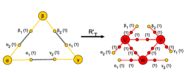
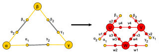
Let us consider a rule RT:lr:subscript𝑅𝑇𝑙𝑟R_{T}:l\rightarrow r which specifies a way to transform a triangle into four triangle graphs. Figure 6 depicts the rule. Black parts should be understood as members of the cut component of the left-hand side, yellow items are in the environment parts. The red items are new in the right-hand side. More precisely, lenvsuperscript𝑙𝑒𝑛𝑣l^{env} consists of 𝒩lenv={α,β,γ}superscriptsubscript𝒩𝑙𝑒𝑛𝑣𝛼𝛽𝛾{\cal N}_{l}^{env}=\{\alpha,\beta,\gamma\}, 𝒫lenv={α1,α2,β1,β2,γ1,γ2}superscriptsubscript𝒫𝑙𝑒𝑛𝑣subscript𝛼1subscript𝛼2subscript𝛽1subscript𝛽2subscript𝛾1subscript𝛾2{\cal P}_{l}^{env}=\{\alpha_{1},\alpha_{2},\beta_{1},\beta_{2},\gamma_{1},\gamma_{2}\}, 𝒫𝒩lenv={(α1,α),(α2,α),(β1,β),(β2,β),{\cal PN}_{l}^{env}=\{(\alpha_{1},\alpha),(\alpha_{2},\alpha),(\beta_{1},\beta),(\beta_{2},\beta), (γ1,γ),(γ2,γ)}(\gamma_{1},\gamma),(\gamma_{2},\gamma)\}, and 𝒫𝒫lenv=𝒫superscriptsubscript𝒫𝑙𝑒𝑛𝑣{\cal PP}_{l}^{env}=\emptyset. The cut component of the left-hand side consists of three port-port connections and their corresponding symmetric connections which will not be written : 𝒫𝒫lcut={(α2,β1),(β2,γ1),(γ2,α1)}𝒫superscriptsubscript𝒫𝑙𝑐𝑢𝑡subscript𝛼2subscript𝛽1subscript𝛽2subscript𝛾1subscript𝛾2subscript𝛼1{\cal PP}_{l}^{cut}=\{(\alpha_{2},\beta_{1}),(\beta_{2},\gamma_{1}),(\gamma_{2},\alpha_{1})\}. The environment component in the right-hand side allows to reconnect the newly introduced items. renvsuperscript𝑟𝑒𝑛𝑣r^{env} consists of the ports 𝒫renv={α1,α2,β1,β2,γ1,γ2}superscriptsubscript𝒫𝑟𝑒𝑛𝑣subscript𝛼1subscript𝛼2subscript𝛽1subscript𝛽2subscript𝛾1subscript𝛾2{\cal P}_{r}^{env}=\{\alpha_{1},\alpha_{2},\beta_{1},\beta_{2},\gamma_{1},\gamma_{2}\}. rnewsuperscript𝑟𝑛𝑒𝑤r^{new} consists of 𝒩rnew={U,V,W}superscriptsubscript𝒩𝑟𝑛𝑒𝑤𝑈𝑉𝑊{\cal N}_{r}^{new}=\{U,V,W\}, 𝒫rnew={u1,u2,u3,u4,v1,v2,v3,v4,w1,w2,w3,w4}superscriptsubscript𝒫𝑟𝑛𝑒𝑤subscript𝑢1subscript𝑢2subscript𝑢3subscript𝑢4subscript𝑣1subscript𝑣2subscript𝑣3subscript𝑣4subscript𝑤1subscript𝑤2subscript𝑤3subscript𝑤4{\cal P}_{r}^{new}=\{u_{1},u_{2},u_{3},u_{4},v_{1},v_{2},v_{3},v_{4},w_{1},w_{2},w_{3},w_{4}\},
𝒫𝒩rnew={(u1,U),(u2,U),(u3,U),(u4,U),(v1,V),(v2,V),(v3,V),(v4,V),(w1,W),(w2,W),(w3,W),(w4,W)}𝒫superscriptsubscript𝒩𝑟𝑛𝑒𝑤subscript𝑢1𝑈subscript𝑢2𝑈subscript𝑢3𝑈subscript𝑢4𝑈subscript𝑣1𝑉subscript𝑣2𝑉subscript𝑣3𝑉subscript𝑣4𝑉subscript𝑤1𝑊subscript𝑤2𝑊subscript𝑤3𝑊subscript𝑤4𝑊{\cal PN}_{r}^{new}=\{(u_{1},U),(u_{2},U),(u_{3},U),(u_{4},U),(v_{1},V),(v_{2},V),(v_{3},V),(v_{4},V),(w_{1},W),(w_{2},W),\\ (w_{3},W),(w_{4},W)\} and 𝒫𝒫rnew={(α1,w2),(α2,u1),(β1,u2),(β2,v1),(γ1,v2),(γ2,w1),(u3,w3),(u4,v4),(w4,v3)}𝒫superscriptsubscript𝒫𝑟𝑛𝑒𝑤subscript𝛼1subscript𝑤2subscript𝛼2subscript𝑢1subscript𝛽1subscript𝑢2subscript𝛽2subscript𝑣1subscript𝛾1subscript𝑣2subscript𝛾2subscript𝑤1subscript𝑢3subscript𝑤3subscript𝑢4subscript𝑣4subscript𝑤4subscript𝑣3{\cal PP}_{r}^{new}=\{(\alpha_{1},w_{2}),(\alpha_{2},u_{1}),(\beta_{1},u_{2}),(\beta_{2},v_{1}),(\gamma_{1},v_{2}),(\gamma_{2},w_{1}),(u_{3},w_{3}),\\ (u_{4},v_{4}),(w_{4},v_{3})\}. The sets of attributes are empty in this example.
Refer to caption
Figure 6: Rule RTsubscript𝑅𝑇R_{T}
Remark 3.

From the definition of an environment sensitive rule, the environment components renv=(𝒩renv,𝒫renv,𝒫𝒩renv,𝒫𝒫renv,𝒜,λrenv)superscript𝑟𝑒𝑛𝑣superscriptsubscript𝒩𝑟𝑒𝑛𝑣superscriptsubscript𝒫𝑟𝑒𝑛𝑣𝒫superscriptsubscript𝒩𝑟𝑒𝑛𝑣𝒫superscriptsubscript𝒫𝑟𝑒𝑛𝑣𝒜superscriptsubscript𝜆𝑟𝑒𝑛𝑣r^{env}=({\cal N}_{r}^{env},{\cal P}_{r}^{env},{\cal PN}_{r}^{env},{\cal PP}_{r}^{env},{\cal A},\lambda_{r}^{env}) and lenv=(𝒩lenv,𝒫lenv,𝒫𝒩lenv,𝒫𝒫lenv,𝒜,λlenv)superscript𝑙𝑒𝑛𝑣superscriptsubscript𝒩𝑙𝑒𝑛𝑣superscriptsubscript𝒫𝑙𝑒𝑛𝑣𝒫superscriptsubscript𝒩𝑙𝑒𝑛𝑣𝒫superscriptsubscript𝒫𝑙𝑒𝑛𝑣𝒜superscriptsubscript𝜆𝑙𝑒𝑛𝑣l^{env}=({\cal N}_{l}^{env},{\cal P}_{l}^{env},{\cal PN}_{l}^{env},{\cal PP}_{l}^{env},{\cal A},\lambda_{l}^{env}) are graphs. However, since 𝒫𝒫lcut𝒫superscriptsubscript𝒫𝑙𝑐𝑢𝑡{\cal PP}_{l}^{cut} may include ports in 𝒫lenvsuperscriptsubscript𝒫𝑙𝑒𝑛𝑣{\cal P}_{l}^{env} and 𝒫𝒩lcut𝒫superscriptsubscript𝒩𝑙𝑐𝑢𝑡{\cal PN}_{l}^{cut} may include nodes in 𝒩lenvsuperscriptsubscript𝒩𝑙𝑒𝑛𝑣{\cal N}_{l}^{env} or ports in 𝒫lenvsuperscriptsubscript𝒫𝑙𝑒𝑛𝑣{\cal P}_{l}^{env}, the cut component lcut=(𝒩lcut,𝒫lcut,𝒫𝒩lcut,𝒫𝒫lcut,𝒜,λlcut)superscript𝑙𝑐𝑢𝑡superscriptsubscript𝒩𝑙𝑐𝑢𝑡superscriptsubscript𝒫𝑙𝑐𝑢𝑡𝒫superscriptsubscript𝒩𝑙𝑐𝑢𝑡𝒫superscriptsubscript𝒫𝑙𝑐𝑢𝑡𝒜superscriptsubscript𝜆𝑙𝑐𝑢𝑡l^{cut}=({\cal N}_{l}^{cut},{\cal P}_{l}^{cut},{\cal PN}_{l}^{cut},{\cal PP}_{l}^{cut},{\cal A},\lambda_{l}^{cut}) is in general neither a graph nor a pregraph. For the same reasons rnew=(𝒩rnew,𝒫rnew,𝒫𝒩rnew,𝒫𝒫rnew,𝒜,λrnew)superscript𝑟𝑛𝑒𝑤superscriptsubscript𝒩𝑟𝑛𝑒𝑤superscriptsubscript𝒫𝑟𝑛𝑒𝑤𝒫superscriptsubscript𝒩𝑟𝑛𝑒𝑤𝒫superscriptsubscript𝒫𝑟𝑛𝑒𝑤𝒜superscriptsubscript𝜆𝑟𝑛𝑒𝑤r^{new}=({\cal N}_{r}^{new},{\cal P}_{r}^{new},{\cal PN}_{r}^{new},{\cal PP}_{r}^{new},\\ {\cal A},\lambda_{r}^{new}) is in general neither a graph nor a pregraph.

Finding an occurrence of a left-hand side of a rule within a graph to be transformed consists in finding a match. This notion is defined below.

Definition 10 (Match).

Let l𝑙l and g𝑔g be two graphs. A match ma:lg:superscript𝑚𝑎𝑙𝑔m^{a}:l\to g is defined as an injective graph homomorphism. a:𝒜l𝒜g:𝑎subscript𝒜𝑙subscript𝒜𝑔a:{\cal A}_{l}\to{\cal A}_{g} being an injective homomorphism over attributes.

Example 5.

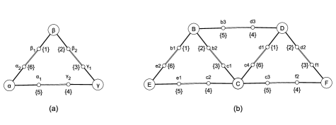
Figure 7 gives a graph l𝑙l and a graph g𝑔g.

Refer to caption
Figure 7: (a) A graph l𝑙l. (b) A graph g𝑔g.

Because of ports attributes, only two matches, m1idsuperscriptsubscript𝑚1𝑖𝑑m_{1}^{id} and m2idsuperscriptsubscript𝑚2𝑖𝑑m_{2}^{id} can be defined from l𝑙l to g𝑔g:

  • m1idsuperscriptsubscript𝑚1𝑖𝑑m_{1}^{id} : m1id(α)=E;m1id(β)=Bformulae-sequencesuperscriptsubscript𝑚1𝑖𝑑𝛼𝐸superscriptsubscript𝑚1𝑖𝑑𝛽𝐵m_{1}^{id}(\alpha)=E;m_{1}^{id}(\beta)=B; m1id(γ)=Csuperscriptsubscript𝑚1𝑖𝑑𝛾𝐶m_{1}^{id}(\gamma)=C; m1id(α1)=e1;m1id(α2)=e2;m1id(β1)=b1;m1id(β2)=b2formulae-sequencesuperscriptsubscript𝑚1𝑖𝑑subscript𝛼1subscript𝑒1formulae-sequencesuperscriptsubscript𝑚1𝑖𝑑subscript𝛼2subscript𝑒2formulae-sequencesuperscriptsubscript𝑚1𝑖𝑑subscript𝛽1subscript𝑏1superscriptsubscript𝑚1𝑖𝑑subscript𝛽2subscript𝑏2m_{1}^{id}(\alpha_{1})=e_{1};m_{1}^{id}(\alpha_{2})=e_{2};m_{1}^{id}(\beta_{1})=b_{1};m_{1}^{id}(\beta_{2})=b_{2}; m1id(γ1)=c1superscriptsubscript𝑚1𝑖𝑑subscript𝛾1subscript𝑐1m_{1}^{id}(\gamma_{1})=c_{1}; m1id(γ2)=c2superscriptsubscript𝑚1𝑖𝑑subscript𝛾2subscript𝑐2m_{1}^{id}(\gamma_{2})=c_{2}.

  • m2idsuperscriptsubscript𝑚2𝑖𝑑m_{2}^{id} : m2id(α)=C;m2id(β)=Dformulae-sequencesuperscriptsubscript𝑚2𝑖𝑑𝛼𝐶superscriptsubscript𝑚2𝑖𝑑𝛽𝐷m_{2}^{id}(\alpha)=C;m_{2}^{id}(\beta)=D; m2id(γ)=Fsuperscriptsubscript𝑚2𝑖𝑑𝛾𝐹m_{2}^{id}(\gamma)=F; m2id(α1)=c3;m2id(α2)=c4;m2id(β1)=d1;m2id(β2)=d2formulae-sequencesuperscriptsubscript𝑚2𝑖𝑑subscript𝛼1subscript𝑐3formulae-sequencesuperscriptsubscript𝑚2𝑖𝑑subscript𝛼2subscript𝑐4formulae-sequencesuperscriptsubscript𝑚2𝑖𝑑subscript𝛽1subscript𝑑1superscriptsubscript𝑚2𝑖𝑑subscript𝛽2subscript𝑑2m_{2}^{id}(\alpha_{1})=c_{3};m_{2}^{id}(\alpha_{2})=c_{4};m_{2}^{id}(\beta_{1})=d_{1};m_{2}^{id}(\beta_{2})=d_{2}; m2id(γ1)=f1superscriptsubscript𝑚2𝑖𝑑subscript𝛾1subscript𝑓1m_{2}^{id}(\gamma_{1})=f_{1}; m2id(γ2)=f2superscriptsubscript𝑚2𝑖𝑑subscript𝛾2subscript𝑓2m_{2}^{id}(\gamma_{2})=f_{2}.

Notice that the occurrences in g𝑔g of m1id(l)superscriptsubscript𝑚1𝑖𝑑𝑙m_{1}^{id}(l) and m2id(l)superscriptsubscript𝑚2𝑖𝑑𝑙m_{2}^{id}(l) overlap on node C𝐶C.

Definition 11 (Rewrite Step).

Let lr𝑙𝑟l\rightarrow r be a rule, g𝑔g a graph and ma:lg:superscript𝑚𝑎𝑙𝑔m^{a}:l\rightarrow g a match. Let l=(𝒩l=𝒩lcut𝒩lenv,𝒫l=𝒫lcut𝒫lenv,𝒫𝒩l=𝒫𝒩lcut𝒫𝒩lenv,𝒫𝒫l=𝒫𝒫lcut𝒫𝒫lenv,𝒜,λl=λlcutλlenv)𝑙formulae-sequencesubscript𝒩𝑙superscriptsubscript𝒩𝑙𝑐𝑢𝑡superscriptsubscript𝒩𝑙𝑒𝑛𝑣formulae-sequencesubscript𝒫𝑙superscriptsubscript𝒫𝑙𝑐𝑢𝑡superscriptsubscript𝒫𝑙𝑒𝑛𝑣formulae-sequence𝒫subscript𝒩𝑙𝒫superscriptsubscript𝒩𝑙𝑐𝑢𝑡𝒫superscriptsubscript𝒩𝑙𝑒𝑛𝑣formulae-sequence𝒫subscript𝒫𝑙𝒫superscriptsubscript𝒫𝑙𝑐𝑢𝑡𝒫superscriptsubscript𝒫𝑙𝑒𝑛𝑣𝒜subscript𝜆𝑙superscriptsubscript𝜆𝑙𝑐𝑢𝑡superscriptsubscript𝜆𝑙𝑒𝑛𝑣l=({\cal N}_{l}={\cal N}_{l}^{cut}\uplus{\cal N}_{l}^{env},{\cal P}_{l}={\cal P}_{l}^{cut}\uplus{\cal P}_{l}^{env},{\cal PN}_{l}={\cal PN}_{l}^{cut}\uplus{\cal PN}_{l}^{env},{\cal PP}_{l}={\cal PP}_{l}^{cut}\uplus{\cal PP}_{l}^{env},{\cal A},\lambda_{l}=\lambda_{l}^{cut}\uplus\lambda_{l}^{env}) and r=(𝒩r=𝒩rnew𝒩renv,𝒫r=𝒫rnew𝒫renv,𝒫𝒩r=𝒫𝒩rnew𝒫𝒩renv,𝒫𝒫r=𝒫𝒫rnew𝒫𝒫renv,𝒜,λr=λrnewλrenv)𝑟formulae-sequencesubscript𝒩𝑟superscriptsubscript𝒩𝑟𝑛𝑒𝑤superscriptsubscript𝒩𝑟𝑒𝑛𝑣formulae-sequencesubscript𝒫𝑟superscriptsubscript𝒫𝑟𝑛𝑒𝑤superscriptsubscript𝒫𝑟𝑒𝑛𝑣formulae-sequence𝒫subscript𝒩𝑟𝒫superscriptsubscript𝒩𝑟𝑛𝑒𝑤𝒫superscriptsubscript𝒩𝑟𝑒𝑛𝑣formulae-sequence𝒫subscript𝒫𝑟𝒫superscriptsubscript𝒫𝑟𝑛𝑒𝑤𝒫superscriptsubscript𝒫𝑟𝑒𝑛𝑣𝒜subscript𝜆𝑟superscriptsubscript𝜆𝑟𝑛𝑒𝑤superscriptsubscript𝜆𝑟𝑒𝑛𝑣r=({\cal N}_{r}={\cal N}_{r}^{new}\uplus{\cal N}_{r}^{env},{\cal P}_{r}={\cal P}_{r}^{new}\uplus{\cal P}_{r}^{env},{\cal PN}_{r}={\cal PN}_{r}^{new}\uplus{\cal PN}_{r}^{env},{\cal PP}_{r}={\cal PP}_{r}^{new}\uplus{\cal PP}_{r}^{env},{\cal A},\lambda_{r}=\lambda_{r}^{new}\uplus\lambda_{r}^{env}). A graph g𝑔g rewrites to gsuperscript𝑔g^{\prime} using a match masuperscript𝑚𝑎m^{a}, written gg𝑔superscript𝑔g\rightarrow g^{\prime} or glr,magsubscript𝑙𝑟superscript𝑚𝑎𝑔superscript𝑔g\rightarrow_{l\rightarrow r,m^{a}}g^{\prime} with gsuperscript𝑔g^{\prime} being a pregraph defined as follows: g=(𝒩g,𝒫g,𝒫𝒩g,𝒫𝒫g,𝒜g,λg)superscript𝑔subscript𝒩superscript𝑔subscript𝒫superscript𝑔𝒫subscript𝒩superscript𝑔𝒫subscript𝒫superscript𝑔subscript𝒜superscript𝑔subscript𝜆superscript𝑔g^{\prime}=({\cal N}_{g^{\prime}},{\cal P}_{g^{\prime}},{\cal PN}_{g^{\prime}},{\cal PP}_{g^{\prime}},{\cal A}_{g^{\prime}},\lambda_{g^{\prime}}) such that

  • 𝒩g=(𝒩g𝒩ma(l)cut)𝒩rnewsubscript𝒩superscript𝑔subscript𝒩𝑔subscriptsuperscript𝒩𝑐𝑢𝑡superscript𝑚𝑎𝑙subscriptsuperscript𝒩𝑛𝑒𝑤𝑟{\cal N}_{g^{\prime}}=({\cal N}_{g}-{\cal N}^{cut}_{m^{a}(l)})\uplus{\cal N}^{new}_{r}

  • 𝒫g=(𝒫g𝒫ma(l)cut)𝒫rnewsubscript𝒫superscript𝑔subscript𝒫𝑔subscriptsuperscript𝒫𝑐𝑢𝑡superscript𝑚𝑎𝑙subscriptsuperscript𝒫𝑛𝑒𝑤𝑟{\cal P}_{g^{\prime}}=({\cal P}_{g}-{\cal P}^{cut}_{m^{a}(l)})\uplus{\cal P}^{new}_{r}

  • 𝒫𝒩g=(𝒫𝒩g𝒫𝒩ma(l)cut)𝒫𝒩ma(r)new𝒫subscript𝒩superscript𝑔𝒫subscript𝒩𝑔𝒫superscriptsubscript𝒩superscript𝑚𝑎𝑙𝑐𝑢𝑡𝒫subscriptsuperscript𝒩𝑛𝑒𝑤superscript𝑚𝑎𝑟{\cal PN}_{g^{\prime}}=({\cal PN}_{g}-{\cal PN}_{m^{a}(l)}^{cut})\uplus{\cal PN}^{new}_{m^{a}(r)}

  • 𝒫𝒫g=(𝒫𝒫g𝒫𝒫ma(l)cut)𝒫𝒫ma(r)new𝒫subscript𝒫superscript𝑔𝒫subscript𝒫𝑔𝒫subscriptsuperscript𝒫𝑐𝑢𝑡superscript𝑚𝑎𝑙𝒫subscriptsuperscript𝒫𝑛𝑒𝑤superscript𝑚𝑎𝑟{\cal PP}_{g^{\prime}}=({\cal PP}_{g}-{\cal PP}^{cut}_{m^{a}(l)})\uplus{\cal PP}^{new}_{m^{a}(r)}

  • 𝒜g=𝒜gsubscript𝒜superscript𝑔subscript𝒜𝑔{\cal A}_{g^{\prime}}={\cal A}_{g} and λg=(λgλma(l)cut)λma(r)newsubscript𝜆superscript𝑔subscript𝜆𝑔subscriptsuperscript𝜆𝑐𝑢𝑡superscript𝑚𝑎𝑙subscriptsuperscript𝜆𝑛𝑒𝑤superscript𝑚𝑎𝑟\lambda_{g^{\prime}}=(\lambda_{g}-\lambda^{cut}_{m^{a}(l)})\uplus\lambda^{new}_{m^{a}(r)}

Notation: Let p,p𝑝superscript𝑝p,p^{\prime} be ports and n𝑛n be a node, in notation ma(r)superscript𝑚𝑎𝑟m^{a}(r) above, ma(p,p)=(ma(p),ma(p))superscript𝑚𝑎𝑝superscript𝑝superscript𝑚𝑎𝑝superscript𝑚𝑎superscript𝑝m^{a}(p,p^{\prime})=(m^{a}(p),m^{a}(p^{\prime})), ma(p,n)=(ma(p),ma(n))superscript𝑚𝑎𝑝𝑛superscript𝑚𝑎𝑝superscript𝑚𝑎𝑛m^{a}(p,n)=(m^{a}(p),m^{a}(n)), ma(p)=psuperscript𝑚𝑎𝑝𝑝m^{a}(p)=p if p𝒫rnew𝑝superscriptsubscript𝒫𝑟𝑛𝑒𝑤p\in{\cal P}_{r}^{new} and ma(n)=nsuperscript𝑚𝑎𝑛𝑛m^{a}(n)=n if n𝒩rnew𝑛superscriptsubscript𝒩𝑟𝑛𝑒𝑤n\in{\cal N}_{r}^{new}.

It is easy to see that graphs are not closed under the rewrite relation defined above. That is to say, when a graph g𝑔g rewrites into gsuperscript𝑔g^{\prime}, gsuperscript𝑔g^{\prime} is a pregraph. To ensure that gsuperscript𝑔g^{\prime} is a graph we provide the following conditions.

Theorem 1.

Let lr𝑙𝑟l\rightarrow r be an environment sensitive rewrite rule, g𝑔g a graph and ma:lg:superscript𝑚𝑎𝑙𝑔m^{a}:l\rightarrow g a match. Let glr,magsubscript𝑙𝑟superscript𝑚𝑎𝑔superscript𝑔g\rightarrow_{l\rightarrow r,m^{a}}g^{\prime}. gsuperscript𝑔g^{\prime} is a graph iff the two following constraints are verified :

  1. 1.

    If p𝒫lenv𝑝superscriptsubscript𝒫𝑙𝑒𝑛𝑣p\in{\cal P}_{l}^{env}, (p,q)𝒫𝒫rnew𝑝𝑞𝒫superscriptsubscript𝒫𝑟𝑛𝑒𝑤(p,q)\in{\cal PP}_{r}^{new} for some port q𝑞q and there is no qsuperscript𝑞q^{\prime} such that (p,q)𝒫𝒫lcut𝑝superscript𝑞𝒫superscriptsubscript𝒫𝑙𝑐𝑢𝑡(p,q^{\prime})\in{\cal PP}_{l}^{cut}, then there is no q′′𝒫gsuperscript𝑞′′subscript𝒫𝑔q^{\prime\prime}\in{\cal P}_{g} such that (ma(p),q′′)𝒫𝒫gsuperscript𝑚𝑎𝑝superscript𝑞′′𝒫subscript𝒫𝑔(m^{a}(p),q^{\prime\prime})\in{\cal PP}_{g}.

  2. 2.

    If p𝒫lenv𝑝superscriptsubscript𝒫𝑙𝑒𝑛𝑣p\in{\cal P}_{l}^{env} , (p,n)𝒫𝒩rnew𝑝𝑛𝒫superscriptsubscript𝒩𝑟𝑛𝑒𝑤(p,n)\in{\cal PN}_{r}^{new} and there is no nsuperscript𝑛n^{\prime} such that (p,n)𝒫𝒩lcut𝑝superscript𝑛𝒫superscriptsubscript𝒩𝑙𝑐𝑢𝑡(p,n^{\prime})\in{\cal PN}_{l}^{cut}, then there is no n′′𝒩gsuperscript𝑛′′subscript𝒩𝑔n^{\prime\prime}\in{\cal N}_{g} such that (ma(p),n′′)𝒫𝒩gsuperscript𝑚𝑎𝑝superscript𝑛′′𝒫subscript𝒩𝑔(m^{a}(p),n^{\prime\prime})\in{\cal PN}_{g}.

Proof.

()(\Leftarrow) Let p𝑝p be a port of gsuperscript𝑔g^{\prime}. If the constraints 1. and 2. are verified then

  • If pgma(r)𝑝superscript𝑔superscript𝑚𝑎𝑟p\in g^{\prime}-m^{a}(r), p𝑝p has the same connections as in g𝑔g. Since g𝑔g is a graph, p𝑝p is connected to at most one port and one node.

  • If pma(renv)𝑝superscript𝑚𝑎superscript𝑟𝑒𝑛𝑣p\in m^{a}(r^{env}), thanks to constraints 1. and 2. p𝑝p has at most one connection to a node and one connection to a port in gsuperscript𝑔g^{\prime}.

  • If p𝒫rnew𝑝superscriptsubscript𝒫𝑟𝑛𝑒𝑤p\in{\cal P}_{r}^{new}. Since r𝑟r is a graph, p𝑝p has at most one connection to a node and one connection to a port in gsuperscript𝑔g^{\prime}.

Thus, gsuperscript𝑔g^{\prime} is a graph.

()(\Rightarrow) It is easy to show, by contrapositive, that in case one of the constraints (1 and 2) is not verified, a counter example can be exhibited.

Matches which fulfill the above two conditions are called well behaved matches.

Example 6.

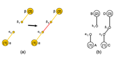
Figure 8 (a) gives an example of toy rule. Figure 8 (b) is a graph H𝐻H such that the match m1idsuperscriptsubscript𝑚1𝑖𝑑m_{1}^{id} as defined below is a well behaved match, whereas the match m2idsuperscriptsubscript𝑚2𝑖𝑑m_{2}^{id} is not a well behaved match. m1id:m1id(α)=A,m1id(β)=B,m1id(α1)=a1,m1id(β1)=b1:superscriptsubscript𝑚1𝑖𝑑formulae-sequencesuperscriptsubscript𝑚1𝑖𝑑𝛼𝐴formulae-sequencesuperscriptsubscript𝑚1𝑖𝑑𝛽𝐵formulae-sequencesuperscriptsubscript𝑚1𝑖𝑑subscript𝛼1subscript𝑎1superscriptsubscript𝑚1𝑖𝑑subscript𝛽1subscript𝑏1m_{1}^{id}:m_{1}^{id}(\alpha)=A,m_{1}^{id}(\beta)=B,m_{1}^{id}(\alpha_{1})=a_{1},m_{1}^{id}(\beta_{1})=b_{1} and m2id:m2id(α)=C,m2id(β)=B,m2id(α1)=c1,m2id(β1)=b1:superscriptsubscript𝑚2𝑖𝑑formulae-sequencesuperscriptsubscript𝑚2𝑖𝑑𝛼𝐶formulae-sequencesuperscriptsubscript𝑚2𝑖𝑑𝛽𝐵formulae-sequencesuperscriptsubscript𝑚2𝑖𝑑subscript𝛼1subscript𝑐1superscriptsubscript𝑚2𝑖𝑑subscript𝛽1subscript𝑏1m_{2}^{id}:m_{2}^{id}(\alpha)=C,m_{2}^{id}(\beta)=B,m_{2}^{id}(\alpha_{1})=c_{1},m_{2}^{id}(\beta_{1})=b_{1}. The application of the toy rule on nodes B𝐵B and C𝐶C and the ports b1subscript𝑏1b_{1} and c1subscript𝑐1c_{1} (according to match m2idsuperscriptsubscript𝑚2𝑖𝑑m_{2}^{id}) leads to a pregraph which is not a graph.
Refer to caption
Figure 8: Example of a toy rule (a) and a graph H𝐻H (b)

In order to define the notion of parallel rewrite step, we have to restrict a bit the class of the considered rewrite systems. Indeed, let l1r1subscript𝑙1subscript𝑟1l_{1}\rightarrow r_{1} and l2r2subscript𝑙2subscript𝑟2l_{2}\rightarrow r_{2} be two ESRR. Applying these two rules in parallel on a graph g𝑔g is possible only if there is “no conflict” while firing the two rules simultaneously. A conflict may occur if some element of the environment of r1envsuperscriptsubscript𝑟1𝑒𝑛𝑣r_{1}^{env} is part of l2cutsuperscriptsubscript𝑙2𝑐𝑢𝑡l_{2}^{cut} and vice versa. To ensure conflict free rewriting, we introduce the notion of conflict free ESRS. Let us first define the notion of compatible rules.

Definition 12 (compatible rules).

Two ESRR’s l1r1subscript𝑙1subscript𝑟1l_{1}\rightarrow r_{1} and l2r2subscript𝑙2subscript𝑟2l_{2}\rightarrow r_{2} are said to be compatible iff for all graphs g𝑔g and matches m1a1:l1g:superscriptsubscript𝑚1subscript𝑎1subscript𝑙1𝑔m_{1}^{a_{1}}:l_{1}\rightarrow g and m2a2:l2g:superscriptsubscript𝑚2subscript𝑎2subscript𝑙2𝑔m_{2}^{a_{2}}:l_{2}\rightarrow g, (i) no element of m1a1(r1env)superscriptsubscript𝑚1subscript𝑎1superscriptsubscript𝑟1𝑒𝑛𝑣m_{1}^{a_{1}}(r_{1}^{env}) is in m2a2(l2cut)superscriptsubscript𝑚2subscript𝑎2superscriptsubscript𝑙2𝑐𝑢𝑡m_{2}^{a_{2}}(l_{2}^{cut}) and (ii) no element of m2a2(r2env)superscriptsubscript𝑚2subscript𝑎2superscriptsubscript𝑟2𝑒𝑛𝑣m_{2}^{a_{2}}(r_{2}^{env}) is in m1a1(l1cut)superscriptsubscript𝑚1subscript𝑎1superscriptsubscript𝑙1𝑐𝑢𝑡m_{1}^{a_{1}}(l_{1}^{cut}).

Conditions (i) and (ii) ensure that the constructions defined by m1a1(r1)superscriptsubscript𝑚1subscript𝑎1subscript𝑟1m_{1}^{a_{1}}(r_{1}) (respectively by m2a2(r2)superscriptsubscript𝑚2subscript𝑎2subscript𝑟2m_{2}^{a_{2}}(r_{2})) can actually be performed ; i.e, no element used in m1a1(r1)superscriptsubscript𝑚1subscript𝑎1subscript𝑟1m_{1}^{a_{1}}(r_{1}) (respectively by m2a2(r2)superscriptsubscript𝑚2subscript𝑎2subscript𝑟2m_{2}^{a_{2}}(r_{2})) is missing because of its inclusion in m2a2(l2cut)superscriptsubscript𝑚2subscript𝑎2superscriptsubscript𝑙2𝑐𝑢𝑡m_{2}^{a_{2}}(l_{2}^{cut}) (respectively in m1a1(l1cut)superscriptsubscript𝑚1subscript𝑎1superscriptsubscript𝑙1𝑐𝑢𝑡m_{1}^{a_{1}}(l_{1}^{cut})). For instance, the reader can easily verify that two variants of the rule

[Uncaptioned image]

are not compatible. Verifying that two given rules are compatible is decidable and can be checked on a finite number, less than max(size(l1),size(l2))𝑚𝑎𝑥𝑠𝑖𝑧𝑒subscript𝑙1𝑠𝑖𝑧𝑒subscript𝑙2max(size(l_{1}),size(l_{2})), of graphs where the size𝑠𝑖𝑧𝑒size of a graph stands for its number of nodes and ports.

Proposition 8.

The problem of the verification of compatibility of two rules is decidable.

Proof.

Let ρ1=l1r1subscript𝜌1subscript𝑙1subscript𝑟1\rho_{1}=l_{1}\rightarrow r_{1} and ρ2=l2r2subscript𝜌2subscript𝑙2subscript𝑟2\rho_{2}=l_{2}\rightarrow r_{2} be two rules. Assume that ρ1subscript𝜌1\rho_{1} and ρ2subscript𝜌2\rho_{2} are not compatible. Then there exists a graph G𝐺G such that:

  • there exists a match m1a1:l1G:superscriptsubscript𝑚1subscript𝑎1subscript𝑙1𝐺m_{1}^{a_{1}}:l_{1}\to G

  • there exists a match m2a2:l2G:superscriptsubscript𝑚2subscript𝑎2subscript𝑙2𝐺m_{2}^{a_{2}}:l_{2}\to G

  • w.l.o.g, we assume that there exists an element, say e𝑒e, in m1a1(r1env)superscriptsubscript𝑚1subscript𝑎1superscriptsubscript𝑟1𝑒𝑛𝑣m_{1}^{a_{1}}(r_{1}^{env}) which belongs also to m2a2(l2cut)superscriptsubscript𝑚2subscript𝑎2superscriptsubscript𝑙2𝑐𝑢𝑡m_{2}^{a_{2}}(l_{2}^{cut}).

Graph G𝐺G can be built as follows: Let d𝑑d be a graph such that there exist two injective homomorphisms h1:dm1a1(l1):subscript1𝑑superscriptsubscript𝑚1subscript𝑎1subscript𝑙1h_{1}:d\rightarrow m_{1}^{a_{1}}(l_{1}) and h2:dm2a2(l2):subscript2𝑑superscriptsubscript𝑚2subscript𝑎2subscript𝑙2h_{2}:d\rightarrow m_{2}^{a_{2}}(l_{2}) such that G𝐺G is obtained as a pushout of h1subscript1h_{1} and h2subscript2h_{2}. That is to say, there exist two injective homomorphisms h1:m1a1(l1)G:subscriptsuperscript1superscriptsubscript𝑚1subscript𝑎1subscript𝑙1𝐺h^{\prime}_{1}:m_{1}^{a_{1}}(l_{1})\to G and h2:m2a2(l2)G:subscriptsuperscript2superscriptsubscript𝑚2subscript𝑎2subscript𝑙2𝐺h^{\prime}_{2}:m_{2}^{a_{2}}(l_{2})\to G such that h1(h1(d))=h2(h2(d))subscriptsuperscript1subscript1𝑑subscriptsuperscript2subscript2𝑑h^{\prime}_{1}(h_{1}(d))=h^{\prime}_{2}(h_{2}(d)). We consider subgraphs d𝑑d which contain at least h11((m1a1)1(e))superscriptsubscript11superscriptsuperscriptsubscript𝑚1subscript𝑎11𝑒h_{1}^{-1}((m_{1}^{a_{1}})^{-1}(e)) which is equal to h21((m2a2)1(e))superscriptsubscript21superscriptsuperscriptsubscript𝑚2subscript𝑎21𝑒h_{2}^{-1}((m_{2}^{a_{2}})^{-1}(e)). Notice that elements of graph d𝑑d could be attributed by empty sets.

Therefore, to check whether two rules ρ1=l1r1subscript𝜌1subscript𝑙1subscript𝑟1\rho_{1}=l_{1}\rightarrow r_{1} and ρ2=l2r2subscript𝜌2subscript𝑙2subscript𝑟2\rho_{2}=l_{2}\rightarrow r_{2} are compatible, one has to check whether there exist a subgraph d𝑑d and two injective homomorphisms h:dl1:𝑑subscript𝑙1h:d\rightarrow l_{1} and h:dl2:superscript𝑑subscript𝑙2h^{\prime}:d\rightarrow l_{2} such that d𝑑d contains an item, e𝑒e, such that h(e)l1cut𝑒superscriptsubscript𝑙1𝑐𝑢𝑡h(e)\in l_{1}^{cut} and h(e)r2envsuperscript𝑒superscriptsubscript𝑟2𝑒𝑛𝑣h^{\prime}(e)\in r_{2}^{env} (h(e)rlenv𝑒superscriptsubscript𝑟𝑙𝑒𝑛𝑣h(e)\in r_{l}^{env} and h(e)l2cutsuperscript𝑒superscriptsubscript𝑙2𝑐𝑢𝑡h^{\prime}(e)\in l_{2}^{cut}) . Since homomorphisms hh and hsuperscripth^{\prime} are injective, the size (number of nodes and ports) of d𝑑d is less than max(size(l1),size(l2))𝑚𝑎𝑥𝑠𝑖𝑧𝑒subscript𝑙1𝑠𝑖𝑧𝑒subscript𝑙2max(size(l_{1}),size(l_{2})). Obviously, d𝑑d, hh and hsuperscripth^{\prime} exist iff the two rules are not compatible. Indeed the graph Gsuperscript𝐺G^{\prime} obtained as a pushout of homomorphisms hh and hsuperscripth^{\prime} contains at least one item which can be matched either by lienvsuperscriptsubscript𝑙𝑖𝑒𝑛𝑣l_{i}^{env} (and remains in rienvsuperscriptsubscript𝑟𝑖𝑒𝑛𝑣r_{i}^{env}) and ljcutsuperscriptsubscript𝑙𝑗𝑐𝑢𝑡l_{j}^{cut} with (i,j){(1,2),(2,1)}𝑖𝑗1221(i,j)\in\{(1,2),(2,1)\}.

Since the set of possible d𝑑d’s is finite (up to isomorphism), verifying whether two rules are compatible is decidable. ∎

Definition 13.

A conflict free environment sensitive graph rewrite system is an ESRS consisting of pairwise compatible rules.

Definition 14 (parallel rewrite step).

Let \mathcal{R} be a conflict free environment sensitive graph rewrite system ={LiRii=1n}conditional-setsubscript𝐿𝑖subscript𝑅𝑖𝑖1𝑛\mathcal{R}=\{L_{i}\rightarrow R_{i}\mid i=1\ldots n\}. Let G𝐺G be a graph. Let I𝐼I be a set of variants of rules in \mathcal{R}, I={lirii=1k}𝐼conditional-setsubscript𝑙𝑖subscript𝑟𝑖𝑖1𝑘I=\{l_{i}\rightarrow r_{i}\mid i=1\ldots k\} and M𝑀M a set of matches M={miai:liGi=1k}𝑀conditional-setsuperscriptsubscript𝑚𝑖subscript𝑎𝑖subscript𝑙𝑖conditional𝐺𝑖1𝑘M=\{m_{i}^{a_{i}}:l_{i}\rightarrow G\mid i=1\dots k\}. We say that graph G𝐺G rewrites into a pregraph Gsuperscript𝐺G^{\prime} using the rules in I𝐼I and matches in M𝑀M, written GI,MGsubscript𝐼𝑀𝐺superscript𝐺G\Rightarrow_{I,M}G^{\prime}, GMGsubscript𝑀𝐺superscript𝐺G\Rightarrow_{M}G^{\prime} or simply GG𝐺superscript𝐺G\Rightarrow G^{\prime} if Gsuperscript𝐺G^{\prime} is obtained following the two steps below:

First step: A pregraph H=(𝒩H,𝒫H,𝒫𝒩H,𝒫𝒫H,𝒜H,λH)𝐻subscript𝒩𝐻subscript𝒫𝐻𝒫subscript𝒩𝐻𝒫subscript𝒫𝐻subscript𝒜𝐻subscript𝜆𝐻H=({\cal N}_{H},{\cal P}_{H},{\cal PN}_{H},{\cal PP}_{H},{\cal A}_{H},\lambda_{H}) is computed using the different matches and rules as follows:

  • 𝒩H=(𝒩Gi=1k𝒩miai(li)cut)i=1k𝒩rinew{\cal N}_{H}=({\cal N}_{G}-\cup_{i=1}^{k}{\cal N}_{m_{i}^{a_{i}}(l_{i})}^{cut})\uplus\cup_{i=1}^{k}{\cal N}_{r_{i}}^{new}

  • 𝒫H=(𝒫Gi=1k𝒫miai(li)cut)i=1k𝒫rinew{\cal P}_{H}=({\cal P}_{G}-\cup_{i=1}^{k}{\cal P}_{m_{i}^{a_{i}}(l_{i})}^{cut})\uplus\cup_{i=1}^{k}{\cal P}_{r_{i}}^{new}

  • 𝒫𝒩H=(𝒫𝒩Gi=1k𝒫𝒩miai(li)cut)i=1k𝒫𝒩miai(ri)new{\cal PN}_{H}=({\cal PN}_{G}-\cup_{i=1}^{k}{\cal PN}_{m_{i}^{a_{i}}(l_{i})}^{cut})\uplus\cup_{i=1}^{k}{\cal PN}_{m_{i}^{a_{i}}(r_{i})}^{new}

  • 𝒫𝒫H=(𝒫𝒫Gi=1k𝒫𝒫miai(li)cut)i=1k𝒫𝒫miai(ri)new{\cal PP}_{H}=({\cal PP}_{G}-\cup_{i=1}^{k}{\cal PP}_{m_{i}^{a_{i}}(l_{i})}^{cut})\uplus\cup_{i=1}^{k}{\cal PP}_{m_{i}^{a_{i}}(r_{i})}^{new}

  • 𝒜H=𝒜Gsubscript𝒜𝐻subscript𝒜𝐺{\cal A}_{H}={\cal A}_{G} and λH=(λGi=1kλmiai(li)cut)i=1nλmiai(ri)new\lambda_{H}=(\lambda_{G}-\cup_{i=1}^{k}\lambda_{m_{i}^{a_{i}}(l_{i})}^{cut})\cup\cup_{i=1}^{n}\lambda_{m_{i}^{a_{i}}(r_{i})}^{new}

second step: G=H¯superscript𝐺¯𝐻G^{\prime}=\overline{H}

Notice that the rewrite step GG𝐺superscript𝐺G\Rightarrow G^{\prime} is a rewrite modulo step [16] of the form GHH¯𝐺𝐻¯𝐻G\to H\equiv\overline{H}.

Example 7.

Let us consider the graph g𝑔g depicted below and the following two matches, m1subscript𝑚1m_{1} and m2subscript𝑚2m_{2}, of the rule RTsubscript𝑅𝑇R_{T} depicted in Figure 6.

[Uncaptioned image]
  • m1subscript𝑚1m_{1} : m1(α)=E;m1(β)=Bformulae-sequencesubscript𝑚1𝛼𝐸subscript𝑚1𝛽𝐵m_{1}(\alpha)=E;m_{1}(\beta)=B; m1(γ)=Csubscript𝑚1𝛾𝐶m_{1}(\gamma)=C; m1(α1)=e1;m1(α2)=e2;m1(β1)=b1;m1(β2)=b2formulae-sequencesubscript𝑚1subscript𝛼1subscript𝑒1formulae-sequencesubscript𝑚1subscript𝛼2subscript𝑒2formulae-sequencesubscript𝑚1subscript𝛽1subscript𝑏1subscript𝑚1subscript𝛽2subscript𝑏2m_{1}(\alpha_{1})=e_{1};m_{1}(\alpha_{2})=e_{2};m_{1}(\beta_{1})=b_{1};m_{1}(\beta_{2})=b_{2}; m1(γ1)=c1subscript𝑚1subscript𝛾1subscript𝑐1m_{1}(\gamma_{1})=c_{1}; m1(γ2)=c2subscript𝑚1subscript𝛾2subscript𝑐2m_{1}(\gamma_{2})=c_{2}. The isomorphism of the port-node and port-port connections are easily deduced.

  • m2subscript𝑚2m_{2} : m2(α)=B;m2(β)=Dformulae-sequencesubscript𝑚2𝛼𝐵subscript𝑚2𝛽𝐷m_{2}(\alpha)=B;m_{2}(\beta)=D; m2(γ)=Csubscript𝑚2𝛾𝐶m_{2}(\gamma)=C; m2(α1)=b2;m2(α2)=b3;m2(β1)=d2;m2(β2)=d1formulae-sequencesubscript𝑚2subscript𝛼1subscript𝑏2formulae-sequencesubscript𝑚2subscript𝛼2subscript𝑏3formulae-sequencesubscript𝑚2subscript𝛽1subscript𝑑2subscript𝑚2subscript𝛽2subscript𝑑1m_{2}(\alpha_{1})=b_{2};m_{2}(\alpha_{2})=b_{3};m_{2}(\beta_{1})=d_{2};m_{2}(\beta_{2})=d_{1}; m2(γ1)=c3subscript𝑚2subscript𝛾1subscript𝑐3m_{2}(\gamma_{1})=c_{3}; m2(γ2)=c1subscript𝑚2subscript𝛾2subscript𝑐1m_{2}(\gamma_{2})=c_{1}.

The two matches overlap.

Figure 9 shows the different steps of the application of two matches of the rule defined in Figure 6. The pregraph, H𝐻H, in the middle is obtained after the first step of Definition 14. Its quotient pregraph, Gsuperscript𝐺G^{\prime}, is the graph on the right. Gsuperscript𝐺G^{\prime} has been obtained by merging the nodes S𝑆S and Y𝑌Y and the ports s1subscript𝑠1s_{1} and y1subscript𝑦1y_{1} as well as ports s2subscript𝑠2s_{2} and y2subscript𝑦2y_{2}. These mergings are depicted by the quotient sets [S],[s1]delimited-[]𝑆delimited-[]subscript𝑠1[S],[s_{1}] and [s2]delimited-[]subscript𝑠2[s_{2}]. For sake of readability, the brackets have been omitted for quotient sets reduced to one element.

Refer to caption

G𝐺G                                  H𝐻H                                  H¯=G¯𝐻superscript𝐺\overline{H}=G^{\prime}

Figure 9: A parallel rewrite step with overlapping between two triangles. Notice that two variants of RTsubscript𝑅𝑇R_{T} with fresh new variables have been provided in order to produce the pregraph H𝐻H. In the quotient graph H¯=G¯𝐻superscript𝐺\overline{H}=G^{\prime}, [S]={S,Y}delimited-[]𝑆𝑆𝑌[S]=\{S,Y\}, [s1]={s1,y1}delimited-[]subscript𝑠1subscript𝑠1subscript𝑦1[s_{1}]=\{s_{1},y_{1}\}, [s2]={s2,y2}delimited-[]subscript𝑠2subscript𝑠2subscript𝑦2[s_{2}]=\{s_{2},y_{2}\}.

As a quotient pregraph is not necessarily a graph (see Figure 5), the above definition of parallel rewrite step does not warranty, in general, the production of graphs only. Hence, we propose hereafter a sufficient condition, which could be verified syntactically, that ensures that the outcome of a parallel rewrite step is still a graph.

Theorem 2.

Let \mathcal{R} be a conflict free environment sensitive graph rewrite system ={LiRii=1n}conditional-setsubscript𝐿𝑖subscript𝑅𝑖𝑖1𝑛\mathcal{R}=\{L_{i}\rightarrow R_{i}\mid i=1\ldots n\}. Let G𝐺G be a graph. Let I𝐼I be a set of variants of rules in \mathcal{R}, I={lirii=1k}𝐼conditional-setsubscript𝑙𝑖subscript𝑟𝑖𝑖1𝑘I=\{l_{i}\rightarrow r_{i}\mid i=1\ldots k\} and M𝑀M a set of matches M={miai:liGi=1k}𝑀conditional-setsuperscriptsubscript𝑚𝑖subscript𝑎𝑖subscript𝑙𝑖conditional𝐺𝑖1𝑘M=\{m_{i}^{a_{i}}:l_{i}\rightarrow G\mid i=1\dots k\}. Let Gsuperscript𝐺G^{\prime} be the pregraph such that GI,MGsubscript𝐼𝑀𝐺superscript𝐺G\Rightarrow_{I,M}G^{\prime}. If p,p𝒫Lienvfor-all𝑝superscript𝑝superscriptsubscript𝒫subscript𝐿𝑖𝑒𝑛𝑣\forall p,p^{\prime}\in{\cal P}_{L_{i}}^{env}, (p,p)𝒫𝒫Rinew𝑝superscript𝑝𝒫superscriptsubscript𝒫subscript𝑅𝑖𝑛𝑒𝑤(p,p^{\prime})\notin{\cal PP}_{R_{i}}^{new}, then Gsuperscript𝐺G^{\prime} is a graph.

Proof.

We have to prove that H𝐻H does not contain odd loops. Because of the previous constraint, it is enough to prove that all ports of H𝐻H are not parts of a loop.

  • If pi=1n𝒫Rinew𝑝superscriptsubscript𝑖1𝑛superscriptsubscript𝒫subscript𝑅𝑖𝑛𝑒𝑤p\in\cup_{i=1}^{n}{\cal P}_{R_{i}}^{new}, it is a new port contained in the graph Risubscript𝑅𝑖R_{i} thus p𝑝p has at most one connection port-port.

  • If pi=1n𝒫miai(Ri)env𝑝superscriptsubscript𝑖1𝑛superscriptsubscript𝒫superscriptsubscript𝑚𝑖subscript𝑎𝑖subscript𝑅𝑖𝑒𝑛𝑣p\in\cup_{i=1}^{n}{\cal P}_{m_{i}^{a_{i}}(R_{i})}^{env}, p𝑝p belongs to the graph G𝐺G and the only new port-port connections where p𝑝p is involved are those of i=1n𝒫Rinewsuperscriptsubscript𝑖1𝑛superscriptsubscript𝒫subscript𝑅𝑖𝑛𝑒𝑤\cup_{i=1}^{n}{\cal P}_{R_{i}}^{new}.

  • Else, if pG/i=1n𝒫Rinewi=1n𝒫miai(Ri)envp\in G/\cup_{i=1}^{n}{\cal P}_{R_{i}}^{new}\uplus\cup_{i=1}^{n}{\cal P}_{m_{i}^{a_{i}}(R_{i})}^{env}, p𝑝p belongs to the non modified part of the graph. Its connections are unchanged and thus p𝑝p has at most one port-port connection.

  • Finally, p𝑝p belongs to a path which is not a loop and H¯=G¯𝐻superscript𝐺\overline{H}=G^{\prime} is a graph.

0.4 Two Parallel Rewrite Relations

The set of matches, M𝑀M, in Definition 14 is not constrained and thus the induced parallel rewrite relation is too nondeterministic since at each step one may choose several sets of matches leading to different rewrite outcomes. In this section, we are rather interested in two confluent parallel rewrite relations which are realistic and can be good candidates for implementations. The first one performs all possible reductions (up to node and port renaming) whereas the second relation is more involved and performs reductions up to left-hand sides’ automorphisms.

0.4.1 Full Parallel Rewrite Relation

We start by a technical definition of an equivalence relation, \approx, over matches.

Definition 15 (\approx).

Let LR𝐿𝑅L\to R be a rule and G𝐺G a graph. Let l1r1subscript𝑙1subscript𝑟1l_{1}\to r_{1} and l2r2subscript𝑙2subscript𝑟2l_{2}\to r_{2} be two variants of the rule LR𝐿𝑅L\to R. We denote by h1a1subscriptsuperscriptsubscript𝑎11h^{a_{1}}_{1} (respect. h2a2subscriptsuperscriptsubscript𝑎22h^{a_{2}}_{2}) the (node, port and attribute) renaming mapping such that the restriction of h1a1subscriptsuperscriptsubscript𝑎11h^{a_{1}}_{1} (respectively, h2a2subscriptsuperscriptsubscript𝑎22h^{a_{2}}_{2}) to Ll1𝐿subscript𝑙1L\to l_{1} (respectively Ll2𝐿subscript𝑙2L\to l_{2}) is a graph isomorphism. Let m1b1:l1G:subscriptsuperscript𝑚subscript𝑏11subscript𝑙1𝐺m^{b_{1}}_{1}:l_{1}\to G and m2b2:l2G:subscriptsuperscript𝑚subscript𝑏22subscript𝑙2𝐺m^{b_{2}}_{2}:l_{2}\to G be two matches. We say that m1b1subscriptsuperscript𝑚subscript𝑏11m^{b_{1}}_{1} and m2b2subscriptsuperscript𝑚subscript𝑏22m^{b_{2}}_{2} are equivalent and write m1b1m2b2subscriptsuperscript𝑚subscript𝑏11subscriptsuperscript𝑚subscript𝑏22m^{b_{1}}_{1}\approx m^{b_{2}}_{2} iff for all elements x𝑥x (in 𝒫Lsubscript𝒫𝐿{\cal P}_{L}, 𝒩Lsubscript𝒩𝐿{\cal N}_{L}, 𝒫𝒫L𝒫subscript𝒫𝐿{\cal PP}_{L} or 𝒫𝒩L𝒫subscript𝒩𝐿{\cal PN}_{L}) of L𝐿L, m1b1(h1a1(x))=m2b2(h2a2(x))subscriptsuperscript𝑚subscript𝑏11subscriptsuperscriptsubscript𝑎11𝑥subscriptsuperscript𝑚subscript𝑏22subscriptsuperscriptsubscript𝑎22𝑥m^{b_{1}}_{1}(h^{a_{1}}_{1}(x))=m^{b_{2}}_{2}(h^{a_{2}}_{2}(x)) and for all x𝑥x in 𝒜Lsubscript𝒜𝐿{\cal A}_{L}, b1(a1(x))=b2(a2(x))subscript𝑏1subscript𝑎1𝑥subscript𝑏2subscript𝑎2𝑥{b_{1}}({a_{1}}(x))={b_{2}}({a_{2}}(x)) .

The relation \approx is clearly an equivalence relation. Intuitively, two matches m1b1:l1G:subscriptsuperscript𝑚subscript𝑏11subscript𝑙1𝐺m^{b_{1}}_{1}:l_{1}\to G and m2b2:l2G:subscriptsuperscript𝑚subscript𝑏22subscript𝑙2𝐺m^{b_{2}}_{2}:l_{2}\to G are equivalent, m1b1m2b2subscriptsuperscript𝑚subscript𝑏11subscriptsuperscript𝑚subscript𝑏22m^{b_{1}}_{1}\approx m^{b_{2}}_{2}, whenever (i) l1subscript𝑙1l_{1} and l2subscript𝑙2l_{2} are left-hand sides of two variants of a same rule, say LR𝐿𝑅L\to R, and (ii) m1b1subscriptsuperscript𝑚subscript𝑏11m^{b_{1}}_{1} and m2b2subscriptsuperscript𝑚subscript𝑏22m^{b_{2}}_{2} coincide on each element x𝑥x of L𝐿L.

Definition 16 (full parallel matches).

Let \mathcal{R} be a graph rewrite system and G𝐺G a graph. Let (G)={miai:liG|miai is a match and liri is a variant of a rule in }subscript𝐺conditional-setsubscriptsuperscript𝑚subscript𝑎𝑖𝑖subscript𝑙𝑖conditional𝐺subscriptsuperscript𝑚subscript𝑎𝑖𝑖 is a match and subscript𝑙𝑖subscript𝑟𝑖 is a variant of a rule in {\cal M}_{\mathcal{R}}(G)=\{m^{a_{i}}_{i}:l_{i}\to G\;|\;m^{a_{i}}_{i}\mbox{ is a match and }l_{i}\to r_{i}\mbox{ is a variant of a rule in }\mathcal{R}\}. A set, M𝑀M, of full parallel matches, with respect to a graph rewrite system \mathcal{R} and a graph G𝐺G, is a maximal set such that (i) M(G)𝑀subscript𝐺M\subset{\cal M}_{{\cal R}}(G) and (ii) m1a1,m2a2M,m1a1m2a2formulae-sequencefor-allsubscriptsuperscript𝑚subscript𝑎11subscriptsuperscript𝑚subscript𝑎22𝑀subscriptsuperscript𝑚subscript𝑎11subscriptsuperscript𝑚subscript𝑎22\forall m^{a_{1}}_{1},m^{a_{2}}_{2}\in M,m^{a_{1}}_{1}\not\approx m^{a_{2}}_{2}.

A set of full parallel matches M𝑀M is not unique because any rule in \mathcal{R} may have infinitely many variants. However the number of non equivalent matches could be easily proven to be finite.

Proposition 9.

Let M𝑀M be a set of full parallel matches with respect to a graph rewrite system \mathcal{R} and a graph G𝐺G. Then M𝑀M is finite.

Proof.

We assume that G𝐺G has a finite number of nodes, ports and attributes and \mathcal{R} has a finite number of rules. Let lirisubscript𝑙𝑖subscript𝑟𝑖l_{i}\to r_{i} be a rule in \mathcal{R}. Let us assume now that nodes and ports of the left-hand side lisubscript𝑙𝑖l_{i} are attributed with the empty set. In this case, matching lisubscript𝑙𝑖l_{i} with subgraphs in G𝐺G remains to find a (non attributed) graph homomorphism between lisubscript𝑙𝑖l_{i} and G𝐺G. Therefore, in this case, the number of possible matches of the left-hand side lisubscript𝑙𝑖l_{i} in graph G𝐺G is at most (kin)×ki!binomialsubscript𝑘𝑖𝑛subscript𝑘𝑖\binom{k_{i}}{n}\times k_{i}! where n=card(𝒩G)+card(𝒫G)𝑛𝑐𝑎𝑟𝑑subscript𝒩𝐺𝑐𝑎𝑟𝑑subscript𝒫𝐺n=card({\cal N}_{G})+card({\cal P}_{G}) and ki=card(𝒩li)+card(𝒫li)subscript𝑘𝑖𝑐𝑎𝑟𝑑subscript𝒩subscript𝑙𝑖𝑐𝑎𝑟𝑑subscript𝒫subscript𝑙𝑖k_{i}=card({\cal N}_{l_{i}})+card({\cal P}_{l_{i}}). Thus card(M)𝑐𝑎𝑟𝑑𝑀card(M) is bounded by Π1icard()(kin)×ki!subscriptΠ1𝑖𝑐𝑎𝑟𝑑binomialsubscript𝑘𝑖𝑛subscript𝑘𝑖\Pi_{1\leq i\leq card(\mathcal{R})}\binom{k_{i}}{n}\times k_{i}! which is finite since n𝑛n and the kisubscript𝑘𝑖k_{i}’s are finite.

Let us consider now the case where lisubscript𝑙𝑖l_{i} is attributed (that is to say, there exists at leat a node or port, say x, such that λli(x)subscript𝜆subscript𝑙𝑖𝑥\lambda_{l_{i}}(x)\not=\emptyset). Let ma:liG:superscript𝑚𝑎subscript𝑙𝑖𝐺m^{a}:l_{i}\to G be a match. m𝑚m is a non-attributed graph homomorphism and a:𝒜li𝒜G:𝑎subscript𝒜subscript𝑙𝑖subscript𝒜𝐺a:{\cal A}_{l_{i}}\to{\cal A}_{G} is an attribute homomorphism which corresponds to a match over attributes in the case where attributes in lisubscript𝑙𝑖l_{i} contain variables. We assume that the matching problem over attributes is finitary. Thus for every m𝑚m there is a finite number, say Cmsubscript𝐶𝑚C_{m}, of possible matchings over attributes a𝑎a. Let lisubscriptsuperscript𝑙𝑖l^{\prime}_{i} be the graph obtained from lisubscript𝑙𝑖l_{i} by removing all attributes (or equivalently said, by setting the attribute function λlisubscript𝜆subscriptsuperscript𝑙𝑖\lambda_{l^{\prime}_{i}} to the empty set. Let Ci=max(Cm|m is a non-attributed graph homomorphism m:liG)C_{i}=max({C_{m}|m\mbox{ is a non-attributed graph homomorphism }m:l^{\prime}_{i}\to G}). Cisubscript𝐶𝑖C_{i} exists since we assume that the matching problem is finitary. Then card(M)𝑐𝑎𝑟𝑑𝑀card(M) is bounded by Π1icard()(kin)×ki!×CisubscriptΠ1𝑖𝑐𝑎𝑟𝑑binomialsubscript𝑘𝑖𝑛subscript𝑘𝑖subscript𝐶𝑖\Pi_{1\leq i\leq card(\mathcal{R})}\binom{k_{i}}{n}\times k_{i}!\times C_{i} which is finite since n𝑛n, the kisubscript𝑘𝑖k_{i}’s and the Cisubscript𝐶𝑖C_{i}’s are finite.

Definition 17 (full parallel rewriting).

Let \mathcal{R} be an ESRS and G𝐺G a graph. Let M𝑀M be a set of full parallel matches with respect to \mathcal{R} and G𝐺G. We define the full parallel rewrite relation and write GMGsubscript𝑀𝐺superscript𝐺G\displaystyle\rightrightarrows_{M}G^{\prime} or simply GG𝐺superscript𝐺G\displaystyle\rightrightarrows G^{\prime}, as the parallel rewrite step GMGsubscript𝑀𝐺superscript𝐺G\Rightarrow_{M}G^{\prime}.

Proposition 10.

Let \mathcal{R} be an ESRS. The rewrite relation \displaystyle\rightrightarrows is deterministic. That is to say, for all graphs g𝑔g, (gg1andgg2)𝑔subscript𝑔1𝑎𝑛𝑑𝑔subscript𝑔2(g\displaystyle\rightrightarrows g_{1}\;and\;g\displaystyle\rightrightarrows g_{2}) implies that g1subscript𝑔1g_{1} and g2subscript𝑔2g_{2} are isomorphic.

Proof.

The proof is quite direct. Let M1subscript𝑀1M_{1} and M2subscript𝑀2M_{2} be two different sets of full parallel matches such that gM1g1subscriptsubscript𝑀1𝑔subscript𝑔1g\displaystyle\rightrightarrows_{M_{1}}g_{1} and gM2g2subscriptsubscript𝑀2𝑔subscript𝑔2g\displaystyle\rightrightarrows_{M_{2}}g_{2}. By definition of sets of full parallel matches, for all matches mbM1superscript𝑚𝑏subscript𝑀1m^{b}\in M_{1} there exists a match mbM2superscript𝑚superscript𝑏subscript𝑀2m^{\prime b^{\prime}}\in{M}_{2} such that mbmbsuperscript𝑚𝑏superscript𝑚superscript𝑏m^{b}\approx m^{\prime b^{\prime}}. Since M1subscript𝑀1M_{1} and M2subscript𝑀2M_{2} are finite (see Proposition 9), there exists a natural number k𝑘k such that M1={m1b1,m2b2,,mkbk}subscript𝑀1superscriptsubscript𝑚1subscript𝑏1superscriptsubscript𝑚2subscript𝑏2superscriptsubscript𝑚𝑘subscript𝑏𝑘M_{1}=\{m_{1}^{b_{1}},m_{2}^{b_{2}},\ldots,m_{k}^{b_{k}}\} and M2={m1b1,m2b2,,mkbk}subscript𝑀2superscriptsubscript𝑚1superscriptsubscript𝑏1superscriptsubscript𝑚2subscriptsuperscript𝑏2superscriptsubscript𝑚𝑘subscriptsuperscript𝑏𝑘M_{2}=\{m_{1}^{\prime b_{1}^{\prime}},m_{2}^{\prime b^{\prime}_{2}},\ldots,m_{k}^{\prime b^{\prime}_{k}}\} such that for all i{1,,k}𝑖1𝑘i\in\{1,\dots,k\}, mibimibisuperscriptsubscript𝑚𝑖subscript𝑏𝑖superscriptsubscript𝑚𝑖subscriptsuperscript𝑏𝑖m_{i}^{b_{i}}\approx m_{i}^{\prime b^{\prime}_{i}}. Therefore, for every i𝑖i such that 1ik1𝑖𝑘1\leq i\leq k, there exist a rule LiRisubscript𝐿𝑖subscript𝑅𝑖L_{i}\to R_{i} in \mathcal{R} and two variants of it lirisubscript𝑙𝑖subscript𝑟𝑖l_{i}\to r_{i} and lirisubscriptsuperscript𝑙𝑖subscriptsuperscript𝑟𝑖l^{\prime}_{i}\to r^{\prime}_{i} together with two renaming mappings hiai:Lili:superscriptsubscript𝑖subscript𝑎𝑖subscript𝐿𝑖subscript𝑙𝑖h_{i}^{a_{i}}:L_{i}\to l_{i} and hiai:Lili:superscriptsubscript𝑖subscriptsuperscript𝑎𝑖subscript𝐿𝑖subscriptsuperscript𝑙𝑖h_{i}^{\prime a^{\prime}_{i}}:L_{i}\to l^{\prime}_{i} such that for all elements xLi𝑥subscript𝐿𝑖x\in L_{i}, mibi(hiai(x))=mibi(hiai(x))superscriptsubscript𝑚𝑖subscript𝑏𝑖superscriptsubscript𝑖subscript𝑎𝑖𝑥superscriptsubscript𝑚𝑖subscriptsuperscript𝑏𝑖superscriptsubscript𝑖subscriptsuperscript𝑎𝑖𝑥m_{i}^{b_{i}}(h_{i}^{a_{i}}(x))=m_{i}^{\prime b^{\prime}_{i}}(h_{i}^{\prime a^{\prime}_{i}}(x)).

By Definitions 14 and 17, graphs g1subscript𝑔1g_{1} and g2subscript𝑔2g_{2} are quotient pregraphs of two pregraphs, respectively H1subscript𝐻1H_{1} and H2subscript𝐻2H_{2}, obtained after the first step of parallel rewrite steps. The sets of nodes and ports of pregraphs H1subscript𝐻1H_{1} and H2subscript𝐻2H_{2} are defined as follows

  • 𝒩H1=(𝒩gi=1k𝒩mibi(li)cut)i=1k𝒩rinew{\cal N}_{H_{1}}=({\cal N}_{g}-\cup_{i=1}^{k}{\cal N}_{m_{i}^{b_{i}}(l_{i})}^{cut})\uplus\cup_{i=1}^{k}{\cal N}_{r_{i}}^{new}

  • 𝒩H2=(𝒩gi=1k𝒩mibi(li)cut)i=1k𝒩rinew{\cal N}_{H_{2}}=({\cal N}_{g}-\cup_{i=1}^{k}{\cal N}_{{m^{\prime}}_{i}^{b^{\prime}_{i}}({l^{\prime}}_{i})}^{cut})\uplus\cup_{i=1}^{k}{\cal N}_{{r^{\prime}}_{i}}^{new}

  • 𝒫H1=(𝒫gi=1k𝒫mibi(li)cut)i=1k𝒫rinew{\cal P}_{H_{1}}=({\cal P}_{g}-\cup_{i=1}^{k}{\cal P}_{m_{i}^{b_{i}}(l_{i})}^{cut})\uplus\cup_{i=1}^{k}{\cal P}_{r_{i}}^{new}

  • 𝒫H2=(𝒫gi=1k𝒫mibi(li)cut)i=1k𝒫rinew{\cal P}_{H_{2}}=({\cal P}_{g}\cup_{i=1}^{k}{\cal P}_{{m^{\prime}}_{i}^{b^{\prime}_{i}}({l^{\prime}}_{i})}^{cut})\uplus\cup_{i=1}^{k}{\cal P}_{{r^{\prime}}_{i}}^{new}

  • λH1=(λgi=1kλmibi(li)cut)i=1kλrinew\lambda_{H_{1}}=(\lambda_{g}-\cup_{i=1}^{k}\lambda_{m_{i}^{b_{i}}(l_{i})}^{cut})\uplus\cup_{i=1}^{k}\lambda_{r_{i}}^{new}

  • λH2=(λgi=1kλmibi(li)cut)i=1kλrinew\lambda_{H_{2}}=(\lambda_{g}-\cup_{i=1}^{k}\lambda_{{m^{\prime}}_{i}^{{b^{\prime}}_{i}}(l_{i})}^{cut})\uplus\cup_{i=1}^{k}\lambda_{r_{i}}^{new}

Now, We define a map fc:H1H2:superscript𝑓𝑐subscript𝐻1subscript𝐻2f^{c}:H_{1}\to H_{2} by means of three maps on nodes, ports and attributes fNc:𝒩H1𝒩H2:subscriptsuperscript𝑓𝑐𝑁subscript𝒩subscript𝐻1subscript𝒩subscript𝐻2f^{c}_{N}:{\cal N}_{H_{1}}\to{\cal N}_{H_{2}}, fPc:𝒫H1𝒫H2:subscriptsuperscript𝑓𝑐𝑃subscript𝒫subscript𝐻1subscript𝒫subscript𝐻2f^{c}_{P}:{\cal P}_{H_{1}}\to{\cal P}_{H_{2}} and c:𝒜H1𝒜H2:𝑐subscript𝒜subscript𝐻1subscript𝒜subscript𝐻2c:{\cal A}_{H_{1}}\to{\cal A}_{H_{2}} as follows

fNc(x)={xif x(𝒩gi=1k𝒩mibi(li)cut)hiai((hiai)1(x))if x𝒩rinew,for 1ikf^{c}_{N}(x)=\begin{cases}x&\text{if }x\in({\cal N}_{g}-\cup_{i=1}^{k}{\cal N}_{m_{i}^{b_{i}}(l_{i})}^{cut})\\ {h^{\prime}}_{i}^{a^{\prime}_{i}}((h^{a_{i}}_{i})^{-1}(x))&\text{if }x\in{\cal N}_{r_{i}}^{new},for\;1\leq i\leq k\end{cases}
fPc(x)={xif x(𝒫gi=1k𝒫mibi(li)cut)hiai((hiai)1(x))if x𝒫rinew,for 1ikf^{c}_{P}(x)=\begin{cases}x&\text{if }x\in({\cal P}_{g}-\cup_{i=1}^{k}{\cal P}_{m_{i}^{b_{i}}(l_{i})}^{cut})\\ {h^{\prime}}_{i}^{a^{\prime}_{i}}((h^{a_{i}}_{i})^{-1}(x))&\text{if }x\in{\cal P}_{r_{i}}^{new},for\;1\leq i\leq k\end{cases}

and c(x)={biaiai1bi1(x)if i{1,,k},e(𝒩H1𝒫H1),(e,x)λrinewxotherwise𝑐𝑥casessuperscriptsubscript𝑏𝑖superscriptsubscript𝑎𝑖superscriptsubscript𝑎𝑖1superscriptsubscript𝑏𝑖1𝑥formulae-sequenceif 𝑖1𝑘formulae-sequence𝑒subscript𝒩subscript𝐻1subscript𝒫subscript𝐻1𝑒𝑥subscriptsuperscript𝜆𝑛𝑒𝑤subscript𝑟𝑖𝑥otherwisec(x)=\begin{cases}b_{i}^{\prime}\circ a_{i}^{\prime}\circ a_{i}^{-1}\circ b_{i}^{-1}(x)&\text{if }\exists i\in\{1,\ldots,k\},\exists e\in({\cal N}_{H_{1}}\cup{\cal P}_{H_{1}}),(e,x)\in\lambda^{new}_{r_{i}}\\ x&\text{otherwise}\end{cases}

fcsuperscript𝑓𝑐f^{c} is clearly a pregraph isomorphism between H1subscript𝐻1H_{1} and H2subscript𝐻2H_{2}. As g1subscript𝑔1g_{1} and g2subscript𝑔2g_{2} are obtained as quotient pregraphs of H1subscript𝐻1H_{1} and H2subscript𝐻2H_{2} respectively, we conclude by using Proposition 6, that g1subscript𝑔1g_{1} and g2subscript𝑔2g_{2} are isomorphic.

Example 8.


[Uncaptioned image]

Let us consider the rule RTsubscript𝑅𝑇R_{T} defined in Figure 6 and the subgraph s𝑠s depicted on the side. The reader can verify that there are six different matches, m1m6subscript𝑚1subscript𝑚6m_{1}\ldots m_{6}, between the left-hand side of RTsubscript𝑅𝑇R_{T} and graph s𝑠s.

These matches are sketched below. Variants of RTsubscript𝑅𝑇R_{T} have been omitted for sake of readability.

  • m1subscript𝑚1m_{1} : m1(α)=E;m1(β)=Bformulae-sequencesubscript𝑚1𝛼𝐸subscript𝑚1𝛽𝐵m_{1}(\alpha)=E;m_{1}(\beta)=B; m1(γ)=Csubscript𝑚1𝛾𝐶m_{1}(\gamma)=C; m1(α1)=e1;m1(α2)=e2;m1(β1)=b1;m1(β2)=b2formulae-sequencesubscript𝑚1subscript𝛼1subscript𝑒1formulae-sequencesubscript𝑚1subscript𝛼2subscript𝑒2formulae-sequencesubscript𝑚1subscript𝛽1subscript𝑏1subscript𝑚1subscript𝛽2subscript𝑏2m_{1}(\alpha_{1})=e_{1};m_{1}(\alpha_{2})=e_{2};m_{1}(\beta_{1})=b_{1};m_{1}(\beta_{2})=b_{2}; m1(γ1)=c1subscript𝑚1subscript𝛾1subscript𝑐1m_{1}(\gamma_{1})=c_{1}; m1(γ2)=c2subscript𝑚1subscript𝛾2subscript𝑐2m_{1}(\gamma_{2})=c_{2}.

  • m2subscript𝑚2m_{2} : m2(α)=E;m2(β)=Cformulae-sequencesubscript𝑚2𝛼𝐸subscript𝑚2𝛽𝐶m_{2}(\alpha)=E;m_{2}(\beta)=C; m2(γ)=Bsubscript𝑚2𝛾𝐵m_{2}(\gamma)=B; m2(α1)=e2;m2(α2)=e1;m2(β1)=c2;m2(β2)=c1formulae-sequencesubscript𝑚2subscript𝛼1subscript𝑒2formulae-sequencesubscript𝑚2subscript𝛼2subscript𝑒1formulae-sequencesubscript𝑚2subscript𝛽1subscript𝑐2subscript𝑚2subscript𝛽2subscript𝑐1m_{2}(\alpha_{1})=e_{2};m_{2}(\alpha_{2})=e_{1};m_{2}(\beta_{1})=c_{2};m_{2}(\beta_{2})=c_{1}; m2(γ1)=b2subscript𝑚2subscript𝛾1subscript𝑏2m_{2}(\gamma_{1})=b_{2}; m2(γ2)=b1subscript𝑚2subscript𝛾2subscript𝑏1m_{2}(\gamma_{2})=b_{1}.

  • m3subscript𝑚3m_{3} : m3(α)=B;m3(β)=Eformulae-sequencesubscript𝑚3𝛼𝐵subscript𝑚3𝛽𝐸m_{3}(\alpha)=B;m_{3}(\beta)=E; m3(γ)=Csubscript𝑚3𝛾𝐶m_{3}(\gamma)=C; m3(α1)=b2;m3(α2)=b1;m3(β1)=e2;m3(β2)=e1formulae-sequencesubscript𝑚3subscript𝛼1subscript𝑏2formulae-sequencesubscript𝑚3subscript𝛼2subscript𝑏1formulae-sequencesubscript𝑚3subscript𝛽1subscript𝑒2subscript𝑚3subscript𝛽2subscript𝑒1m_{3}(\alpha_{1})=b_{2};m_{3}(\alpha_{2})=b_{1};m_{3}(\beta_{1})=e_{2};m_{3}(\beta_{2})=e_{1}; m3(γ1)=c2subscript𝑚3subscript𝛾1subscript𝑐2m_{3}(\gamma_{1})=c_{2}; m3(γ2)=c1subscript𝑚3subscript𝛾2subscript𝑐1m_{3}(\gamma_{2})=c_{1}.

  • m4subscript𝑚4m_{4} : m4(α)=B;m4(β)=Cformulae-sequencesubscript𝑚4𝛼𝐵subscript𝑚4𝛽𝐶m_{4}(\alpha)=B;m_{4}(\beta)=C; m4(γ)=Esubscript𝑚4𝛾𝐸m_{4}(\gamma)=E; m4(α1)=b1;m4(α2)=b2;m4(β1)=c1;m4(β2)=c2formulae-sequencesubscript𝑚4subscript𝛼1subscript𝑏1formulae-sequencesubscript𝑚4subscript𝛼2subscript𝑏2formulae-sequencesubscript𝑚4subscript𝛽1subscript𝑐1subscript𝑚4subscript𝛽2subscript𝑐2m_{4}(\alpha_{1})=b_{1};m_{4}(\alpha_{2})=b_{2};m_{4}(\beta_{1})=c_{1};m_{4}(\beta_{2})=c_{2}; m3(γ1)=e1subscript𝑚3subscript𝛾1subscript𝑒1m_{3}(\gamma_{1})=e_{1}; m4(γ2)=e2subscript𝑚4subscript𝛾2subscript𝑒2m_{4}(\gamma_{2})=e_{2}.

  • m5subscript𝑚5m_{5} : m5(α)=C;m5(β)=Bformulae-sequencesubscript𝑚5𝛼𝐶subscript𝑚5𝛽𝐵m_{5}(\alpha)=C;m_{5}(\beta)=B; m5(γ)=Esubscript𝑚5𝛾𝐸m_{5}(\gamma)=E; m5(α1)=c2;m5(α2)=c1;m5(β1)=b2;m5(β2)=b1formulae-sequencesubscript𝑚5subscript𝛼1subscript𝑐2formulae-sequencesubscript𝑚5subscript𝛼2subscript𝑐1formulae-sequencesubscript𝑚5subscript𝛽1subscript𝑏2subscript𝑚5subscript𝛽2subscript𝑏1m_{5}(\alpha_{1})=c_{2};m_{5}(\alpha_{2})=c_{1};m_{5}(\beta_{1})=b_{2};m_{5}(\beta_{2})=b_{1}; m5(γ1)=e2subscript𝑚5subscript𝛾1subscript𝑒2m_{5}(\gamma_{1})=e_{2}; m5(γ2)=e1subscript𝑚5subscript𝛾2subscript𝑒1m_{5}(\gamma_{2})=e_{1}.

  • m6subscript𝑚6m_{6} : m5(α)=C;m5(β)=Eformulae-sequencesubscript𝑚5𝛼𝐶subscript𝑚5𝛽𝐸m_{5}(\alpha)=C;m_{5}(\beta)=E; m5(γ)=Bsubscript𝑚5𝛾𝐵m_{5}(\gamma)=B; m5(α1)=c1;m5(α2)=c2;m5(β1)=e1;m5(β2)=e2formulae-sequencesubscript𝑚5subscript𝛼1subscript𝑐1formulae-sequencesubscript𝑚5subscript𝛼2subscript𝑐2formulae-sequencesubscript𝑚5subscript𝛽1subscript𝑒1subscript𝑚5subscript𝛽2subscript𝑒2m_{5}(\alpha_{1})=c_{1};m_{5}(\alpha_{2})=c_{2};m_{5}(\beta_{1})=e_{1};m_{5}(\beta_{2})=e_{2}; m5(γ1)=b1subscript𝑚5subscript𝛾1subscript𝑏1m_{5}(\gamma_{1})=b_{1}; m5(γ2)=b2subscript𝑚5subscript𝛾2subscript𝑏2m_{5}(\gamma_{2})=b_{2}.

Here, the homomorphisms over attributes are always the identity, that is why they have been omitted. Thanks to the six matches and the rule RTsubscript𝑅𝑇R_{T}, the reader may check that the subgraph s𝑠s can be rewritten, by using six different variants of rule RTsubscript𝑅𝑇R_{T}, into a pregraph containing 3×6363\times 6 new nodes and 12×612612\times 6 new ports. The quotient pregraph has only 333 new nodes but has 424242 new ports. Each pair of new nodes has 666 connections.

This example shows that the full parallel rewriting has to be used carefully since it may produce non intended results due to overmatching the same subgraphs. To overcome this issue, one may use attributes in order to lower the possible matches. We call such attributes distinguishing attributes.
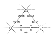
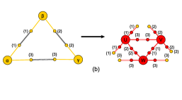
Refer to caption
Refer to caption
Figure 10: (a) Subgraph s𝑠s with distinguishing attributes on ports. The attributes are {1,2,3}123\{1,2,3\}. (b) Rule RTsubscript𝑅𝑇R_{T} with distinguishing attributes.

In order to consider only one match of the subgraph s𝑠s considered in Example 8 by the rule RTsubscript𝑅𝑇R_{T}, one option is to apply full parallel rewrite relation with distinguishing attributes on the subgraph depicted in Figure 10 (a) and rule RTsubscript𝑅𝑇R_{T} with distinguishing attributes given in Figure 10 (b), leading to a pregraph whose quotient is a graph with 333 new nodes and 121212 new ports. This graph is the expected one.

Another way to mitigate the problems of overmatching subgraphs, in addition to the use of distinguishing attributes, consists in taking advantage of the symmetries that appear in the graphs of rewrite rules. This leads us to define a new rewrite relation which gets rid of multiple matches of the same left-hand-side of a fixed rule. We call this relation parallel up to automorphisms and is defined below.

0.4.2 Parallel Rewrite Relation up to Automorphisms

Let us consider a graph g𝑔g which rewrites into g1subscript𝑔1g_{1} and g2subscript𝑔2g_{2} using an ESRR lr𝑙𝑟l\to r. This means that there exist two matches μiβi:lg:subscriptsuperscript𝜇subscript𝛽𝑖𝑖𝑙𝑔\mu^{\beta_{i}}_{i}:l\to g with i{1,2}𝑖12i\in\{1,2\} such that glr,μiβigisubscript𝑙𝑟subscriptsuperscript𝜇subscript𝛽𝑖𝑖𝑔subscript𝑔𝑖g\Rightarrow_{l\rightarrow r,\mu^{\beta_{i}}_{i}}g_{i}. One may wonder whether g1subscript𝑔1g_{1} and g2subscript𝑔2g_{2} are the same (up to isomorphism) whenever matches μ1β1subscriptsuperscript𝜇subscript𝛽11\mu^{\beta_{1}}_{1} and μ2β2subscriptsuperscript𝜇subscript𝛽22\mu^{\beta_{2}}_{2} are linked by means of an automorphism of l𝑙l. That is to say, when there exists an automorphism ha:ll:superscript𝑎𝑙𝑙h^{a}:l\to l with μ1β1=μ2β2hasubscriptsuperscript𝜇subscript𝛽11subscriptsuperscript𝜇subscript𝛽22superscript𝑎\mu^{\beta_{1}}_{1}=\mu^{\beta_{2}}_{2}\circ h^{a}. Intuitively, matches μ1β1subscriptsuperscript𝜇subscript𝛽11\mu^{\beta_{1}}_{1} and μ2β2subscriptsuperscript𝜇subscript𝛽22\mu^{\beta_{2}}_{2} could be considered as the same up to a permutation of nodes. We show below that g1subscript𝑔1g_{1} and g2subscript𝑔2g_{2} are actually isomorphic but under some syntactic condition we call symmetry condition.

Notation: Let g𝑔g be a graph with attributes in 𝒜𝒜{\cal A}. We write H(g)𝐻𝑔H(g) to denote the set of automorphisms of g𝑔g, i.e. H(g)𝐻𝑔H(g) is the set of isomorphisms ha:gg:superscript𝑎𝑔𝑔h^{a}:g\to g, with a𝑎a being an isomorphism on the attributes of g𝑔g, a:𝒜𝒜:𝑎𝒜𝒜a:{\cal A}\to{\cal A}.

Proposition 11.

Let lr𝑙𝑟l\to r be an ESRR. let l1r1subscript𝑙1subscript𝑟1l_{1}\to r_{1} and l2r2subscript𝑙2subscript𝑟2l_{2}\to r_{2} be two variants of the rule lr𝑙𝑟l\to r. Let v1c1superscriptsubscript𝑣1subscript𝑐1v_{1}^{c_{1}}, v1c1superscriptsubscript𝑣1subscript𝑐1v_{1}^{\prime c_{1}}, v2c2superscriptsubscript𝑣2subscript𝑐2v_{2}^{c_{2}}, v2c2superscriptsubscript𝑣2subscript𝑐2v_{2}^{\prime c_{2}} be the isomorphisms reflecting the variant status of these two rules with v1c1:ll1:superscriptsubscript𝑣1subscript𝑐1𝑙subscript𝑙1v_{1}^{c_{1}}:l\to l_{1}, v1c1:rr1:superscriptsubscript𝑣1subscript𝑐1𝑟subscript𝑟1v_{1}^{\prime c_{1}}:r\to r_{1}, v2c2:ll2:superscriptsubscript𝑣2subscript𝑐2𝑙subscript𝑙2v_{2}^{c_{2}}:l\to l_{2} and v2c2:rr2:superscriptsubscript𝑣2subscript𝑐2𝑟subscript𝑟2v_{2}^{\prime c_{2}}:r\to r_{2} such that li=vici(l)subscript𝑙𝑖superscriptsubscript𝑣𝑖subscript𝑐𝑖𝑙l_{i}=v_{i}^{c_{i}}(l), ri=vici(r)subscript𝑟𝑖superscriptsubscript𝑣𝑖subscript𝑐𝑖𝑟r_{i}=v_{i}^{\prime c_{i}}(r) and vici(rienv)=vici(rienv)superscriptsubscript𝑣𝑖subscript𝑐𝑖superscriptsubscript𝑟𝑖𝑒𝑛𝑣superscriptsubscript𝑣𝑖subscript𝑐𝑖superscriptsubscript𝑟𝑖𝑒𝑛𝑣v_{i}^{c_{i}}(r_{i}^{env})=v_{i}^{\prime c_{i}}(r_{i}^{env}) for i{1,2}𝑖12i\in\{1,2\}. Let g𝑔g be a graph and g1subscriptsuperscript𝑔1g^{\prime}_{1} and g2subscriptsuperscript𝑔2g^{\prime}_{2} be two pregraphs. Let gl1r1,m1b1g1subscriptsubscript𝑙1subscript𝑟1subscriptsuperscript𝑚subscript𝑏11𝑔superscriptsubscript𝑔1g\Rightarrow_{l_{1}\rightarrow r_{1},m^{b_{1}}_{1}}g_{1}^{\prime} and gl2r2,m2b2g2subscriptsubscript𝑙2subscript𝑟2subscriptsuperscript𝑚subscript𝑏22𝑔superscriptsubscript𝑔2g\Rightarrow_{l_{2}\rightarrow r_{2},m^{b_{2}}_{2}}g_{2}^{\prime} be two rewrite steps such that there exist two automorphisms ha:ll:superscript𝑎𝑙𝑙h^{a}:l\to l and ha:rr:superscript𝑎𝑟𝑟h^{\prime a}:r\to r such that (i) with m1b1=m2b2v2c2ha(v1c1)1subscriptsuperscript𝑚subscript𝑏11subscriptsuperscript𝑚subscript𝑏22superscriptsubscript𝑣2subscript𝑐2superscript𝑎superscriptsuperscriptsubscript𝑣1subscript𝑐11m^{b_{1}}_{1}=m^{b_{2}}_{2}\circ v_{2}^{c_{2}}\circ h^{a}\circ(v_{1}^{c_{1}})^{-1} and (ii) for all elements x𝑥x of renvsuperscript𝑟𝑒𝑛𝑣r^{env}, ha(x)=ha(x)superscript𝑎𝑥superscript𝑎𝑥h^{\prime a}(x)=h^{a}(x). Then, g1superscriptsubscript𝑔1g_{1}^{\prime} and g2superscriptsubscript𝑔2g_{2}^{\prime} are isomorphic.

Sketch.

The sketch of the proof is depicted in Figure 11. The attributes structures used in the rule lr𝑙𝑟l\to r (respectively, l1r1subscript𝑙1subscript𝑟1l_{1}\to r_{1} and l2r2subscript𝑙2subscript𝑟2l_{2}\to r_{2}) are denoted A𝐴A (respectively, A1subscript𝐴1A_{1} and A2subscript𝐴2A_{2}) whereas the attibutes structure of the transfomed graph g𝑔g is denoted B𝐵B. From the hypotheses, we can easily infer the exitence of two isomorphisms hvcv:l1l2:superscriptsubscript𝑣subscript𝑐𝑣subscript𝑙1subscript𝑙2h_{v}^{c_{v}}:l_{1}\to l_{2} and hvcv:r1r2:superscriptsubscript𝑣subscript𝑐𝑣subscript𝑟1subscript𝑟2h_{v}^{\prime c_{v}}:r_{1}\to r_{2} such that hvcv=v2c2ha(v1c1)1superscriptsubscript𝑣subscript𝑐𝑣superscriptsubscript𝑣2subscript𝑐2superscript𝑎superscriptsuperscriptsubscript𝑣1subscript𝑐11h_{v}^{c_{v}}=v_{2}^{c_{2}}\circ h^{a}\circ(v_{1}^{c_{1}})^{-1} and hvcv=v2cvha(v1c1)1superscriptsubscript𝑣subscript𝑐𝑣superscriptsubscript𝑣2subscript𝑐𝑣superscript𝑎superscriptsuperscriptsubscript𝑣1subscript𝑐11h_{v}^{\prime c_{v}}=v_{2}^{\prime c_{v}}\circ h^{\prime a}\circ(v_{1}^{\prime c_{1}})^{-1}. And we have cv=c2ac11subscript𝑐𝑣subscript𝑐2𝑎superscriptsubscript𝑐11c_{v}=c_{2}\circ a\circ c_{1}^{-1}.

Let gl1r1,m1b1g1subscriptsubscript𝑙1subscript𝑟1superscriptsubscript𝑚1subscript𝑏1𝑔superscriptsubscript𝑔1g\Rightarrow_{l_{1}\rightarrow r_{1},m_{1}^{b_{1}}}g_{1}^{\prime} and gl2r2,m2b2g2subscriptsubscript𝑙2subscript𝑟2superscriptsubscript𝑚2subscript𝑏2𝑔superscriptsubscript𝑔2g\Rightarrow_{l_{2}\rightarrow r_{2},m_{2}^{b_{2}}}g_{2}^{\prime} such that m1b1(l1)=m2b2(l2)superscriptsubscript𝑚1subscript𝑏1subscript𝑙1superscriptsubscript𝑚2subscript𝑏2subscript𝑙2m_{1}^{b_{1}}(l_{1})=m_{2}^{b_{2}}(l_{2}). By definition of a rewrite step, there exist a pregraph g1subscript𝑔1g_{1} (respect. a pregraph g2subscript𝑔2g_{2}) and an injective homomorphism m1b1:r1g1:superscriptsubscript𝑚1subscript𝑏1subscript𝑟1subscript𝑔1m_{1}^{\prime b_{1}}:r_{1}\to g_{1} (respect. m2b2:r2g2:superscriptsubscript𝑚2subscript𝑏2subscript𝑟2subscript𝑔2m_{2}^{\prime b_{2}}:r_{2}\to g_{2}) such that g1=g¯1subscriptsuperscript𝑔1subscript¯𝑔1g^{\prime}_{1}=\overline{g}_{1} (respect. g2=g¯2subscriptsuperscript𝑔2subscript¯𝑔2g^{\prime}_{2}=\overline{g}_{2}). Moreover, since, by definition, renvsuperscript𝑟𝑒𝑛𝑣r^{env} is included in lenvsuperscript𝑙𝑒𝑛𝑣l^{env} for any ESRR lr𝑙𝑟l\to r, we have m1b1(r1env)=m1b1(r1env)superscriptsubscript𝑚1subscript𝑏1superscriptsubscript𝑟1𝑒𝑛𝑣superscriptsubscript𝑚1subscript𝑏1superscriptsubscript𝑟1𝑒𝑛𝑣m_{1}^{\prime b_{1}}(r_{1}^{env})=m_{1}^{b_{1}}(r_{1}^{env}) (respect. m2b2(r2env)=m2b2(r2env)superscriptsubscript𝑚2subscript𝑏2superscriptsubscript𝑟2𝑒𝑛𝑣superscriptsubscript𝑚2subscript𝑏2superscriptsubscript𝑟2𝑒𝑛𝑣m_{2}^{\prime b_{2}}(r_{2}^{env})=m_{2}^{b_{2}}(r_{2}^{env})), where mibisuperscriptsubscript𝑚𝑖subscript𝑏𝑖m_{i}^{\prime b_{i}}, for i{1,2}𝑖12i\in\{1,2\}, are defined as follows:

for n𝒩ri,mibi(n)={mibi(n)ifn𝒩rienvnotherwise(n𝒩rinew)formulae-sequence𝑛subscript𝒩subscript𝑟𝑖subscriptsuperscriptsuperscript𝑚subscript𝑏𝑖𝑖𝑛casessubscriptsuperscript𝑚subscript𝑏𝑖𝑖𝑛𝑖𝑓𝑛superscriptsubscript𝒩subscript𝑟𝑖𝑒𝑛𝑣𝑛𝑜𝑡𝑒𝑟𝑤𝑖𝑠𝑒𝑛superscriptsubscript𝒩subscript𝑟𝑖𝑛𝑒𝑤n\in{\cal N}_{r_{i}},{m^{\prime}}^{b_{i}}_{i}(n)=\left\{\begin{array}[]{l}m^{b_{i}}_{i}(n)\;if\;n\in{\cal N}_{r_{i}}^{env}\\ n\;otherwise(n\in{\cal N}_{r_{i}}^{new})\end{array}\right.

for p𝒫ri,mibi(p)={mibi(p)ifp𝒫rienvpotherwise(p𝒫rinew)formulae-sequence𝑝subscript𝒫subscript𝑟𝑖subscriptsuperscriptsuperscript𝑚subscript𝑏𝑖𝑖𝑝casessubscriptsuperscript𝑚subscript𝑏𝑖𝑖𝑝𝑖𝑓𝑝superscriptsubscript𝒫subscript𝑟𝑖𝑒𝑛𝑣𝑝𝑜𝑡𝑒𝑟𝑤𝑖𝑠𝑒𝑝superscriptsubscript𝒫subscript𝑟𝑖𝑛𝑒𝑤p\in{\cal P}_{r_{i}},{m^{\prime}}^{b_{i}}_{i}(p)=\left\{\begin{array}[]{l}m^{b_{i}}_{i}(p)\;if\;p\in{\cal P}_{r_{i}}^{env}\\ p\;otherwise(p\in{\cal P}_{r_{i}}^{new})\end{array}\right.

Now, let us define the isomorphism h′′d:g1g2:superscript′′𝑑subscript𝑔1subscript𝑔2h^{\prime\prime d}:g_{1}\to g_{2} with d(x)=𝑑𝑥absentd(x)= if xb1(A1)𝑥subscript𝑏1subscript𝐴1x\in b_{1}(A_{1}) then b2cvb11(x)subscript𝑏2subscript𝑐𝑣superscriptsubscript𝑏11𝑥b_{2}\circ c_{v}\circ b_{1}^{-1}(x) else x𝑥x. Let us consider x𝑥x such that x𝑥x is an element of renvsuperscript𝑟𝑒𝑛𝑣r^{env} (port or node). We have m1b1(v1c1(x))=m2b2(v2c2(ha(x)))superscriptsubscript𝑚1subscript𝑏1superscriptsubscript𝑣1subscript𝑐1𝑥superscriptsubscript𝑚2subscript𝑏2superscriptsubscript𝑣2subscript𝑐2superscript𝑎𝑥m_{1}^{b_{1}}(v_{1}^{c_{1}}(x))=m_{2}^{b_{2}}(v_{2}^{c_{2}}(h^{a}(x))) is an element of g𝑔g. Moreover m1b1(v1c1(x))g1superscriptsubscript𝑚1subscript𝑏1superscriptsubscript𝑣1subscript𝑐1𝑥subscript𝑔1m_{1}^{\prime b_{1}}(v_{1}^{\prime c_{1}}(x))\in g_{1} and m2b2(v2c2(ha(x))g2m_{2}^{\prime b_{2}}(v_{2}^{\prime c_{2}}({h^{\prime}}^{a}(x))\in g_{2}. Let us denote y=m1b1(v1c1(x))𝑦superscriptsubscript𝑚1subscript𝑏1superscriptsubscript𝑣1subscript𝑐1𝑥y=m_{1}^{b_{1}}(v_{1}^{c_{1}}(x)). By construction m1b1(v1c1(x))=m1b1(v1c1(x))=ysuperscriptsubscript𝑚1subscript𝑏1superscriptsubscript𝑣1subscript𝑐1𝑥superscriptsubscript𝑚1subscript𝑏1superscriptsubscript𝑣1subscript𝑐1𝑥𝑦m_{1}^{\prime b_{1}}(v_{1}^{\prime c_{1}}(x))=m_{1}^{b_{1}}(v_{1}^{c_{1}}(x))=y because xrenv𝑥superscript𝑟𝑒𝑛𝑣x\in r^{env}. From the hypothesis we have ha(x)=ha(x)superscript𝑎𝑥superscriptsuperscript𝑎𝑥h^{a}(x)={h^{\prime}}^{a}(x). Thus m2b2(v2c2(ha(x))=m2b2(v2c2(ha(x))m_{2}^{\prime b_{2}}(v_{2}^{\prime c_{2}}({h^{\prime}}^{a}(x))=m_{2}^{\prime b_{2}}(v_{2}^{\prime c_{2}}(h^{a}(x)) and then we have m2b2(v2c2(ha(x))=m2b2(v2c2(ha(x))=ym_{2}^{\prime b_{2}}(v_{2}^{\prime c_{2}}({h^{\prime}}^{a}(x))=m_{2}^{b_{2}}(v_{2}^{c_{2}}(h^{a}(x))=y. Then, for all elements z𝑧z of the non-modified part of g𝑔g which is gm1b1(v1c1(l))𝑔superscriptsubscript𝑚1subscript𝑏1superscriptsubscript𝑣1subscript𝑐1𝑙g-m_{1}^{b_{1}}(v_{1}^{c_{1}}(l)) (z𝑧z can be a port or a node if y𝑦y is not a node) such that (z,y)g𝑧𝑦𝑔(z,y)\in g, we have that (z,y)g1𝑧𝑦subscript𝑔1(z,y)\in g_{1} and (z,y)g2𝑧𝑦subscript𝑔2(z,y)\in g_{2} and h′′d=Iddsuperscriptsuperscript′′𝑑𝐼superscript𝑑𝑑{h^{\prime\prime}}^{d}=Id^{d} on g1m1b1(v1c1(r))subscript𝑔1superscriptsubscript𝑚1subscript𝑏1superscriptsubscript𝑣1subscript𝑐1𝑟g_{1}-m_{1}^{\prime b_{1}}(v_{1}^{\prime c_{1}}(r)). Finally the definition of h′′dsuperscript′′𝑑h^{\prime\prime d} is :

For y𝒩g1𝒫g1,h′′d(y)={m2b2(hvcv((m1b1)1(y)))ifym1b1(r1)yotherwiseformulae-sequence𝑦subscript𝒩subscript𝑔1subscript𝒫subscript𝑔1superscript′′𝑑𝑦casessuperscriptsubscript𝑚2subscript𝑏2superscriptsubscript𝑣subscript𝑐𝑣superscriptsuperscriptsubscript𝑚1subscript𝑏11𝑦𝑖𝑓𝑦superscriptsubscript𝑚1subscript𝑏1subscript𝑟1𝑦𝑜𝑡𝑒𝑟𝑤𝑖𝑠𝑒y\in{\cal N}_{g_{1}}\cup{\cal P}_{g_{1}},h^{\prime\prime d}(y)=\left\{\begin{array}[]{l}m_{2}^{\prime b_{2}}(h_{v}^{\prime c_{v}}((m_{1}^{\prime b_{1}})^{-1}(y)))\;if\;y\in m_{1}^{\prime b_{1}}(r_{1})\\ y\;otherwise\end{array}\right.

For all types of existing connections (y,z)𝑦𝑧(y,z) of g1subscript𝑔1g_{1} where y𝑦y and z𝑧z in 𝒩g1𝒫g1subscript𝒩subscript𝑔1subscript𝒫subscript𝑔1{\cal N}_{g_{1}}\cup{\cal P}_{g_{1}}, h′′d(y,z)=(h′′d(y),h′′d(z))superscript′′𝑑𝑦𝑧superscript′′𝑑𝑦superscript′′𝑑𝑧h^{\prime\prime d}(y,z)=(h^{\prime\prime d}(y),h^{\prime\prime d}(z)) is in g2subscript𝑔2g_{2}. By construction, the homomorphism conditions on attributes are fulfilled by h′′dsuperscript′′𝑑h^{\prime\prime d}. Thus, h′′d:g1g2:superscript′′𝑑subscript𝑔1subscript𝑔2h^{\prime\prime d}:g_{1}\to g_{2} is a pregraph homomorphism. In addition, h′′dsuperscript′′𝑑h^{\prime\prime d} is bijective by construction. From h′′dsuperscript′′𝑑h^{\prime\prime d} and Proposition 6, we infer the isomorphism h(3)d:g1g2:superscript3𝑑subscriptsuperscript𝑔1subscriptsuperscript𝑔2h^{(3)d}:g^{\prime}_{1}\to g^{\prime}_{2}.

Refer to caption
Refer to caption
Figure 11: Sketch of the proof of Proposition 11

Definition 18 (Symmetry Condition).

An ESRR lr𝑙𝑟l\rightarrow r verifies the symmetry condition  iff haH(l),haH(r),such thatxrenv,ha(x)=ha(x)formulae-sequencefor-allsuperscript𝑎𝐻𝑙formulae-sequencesuperscript𝑎𝐻𝑟formulae-sequencesuch thatfor-all𝑥superscript𝑟𝑒𝑛𝑣superscript𝑎𝑥superscript𝑎𝑥\forall h^{a}\in H(l),\;\exists\;h^{\prime a}\in H(r),\;\mbox{such that}\;\forall x\in r^{env},h^{a}(x)=h^{\prime a}(x)

The reader can check that the rule RTsubscript𝑅𝑇R_{T} verifies the symmetry condition.

Definition 19 (Matches up to automorphism, lsuperscriptsimilar-to𝑙\sim^{l}).

Let lr𝑙𝑟l\to r be an ESRR satisfying the symmetry condition. Let l1r1subscript𝑙1subscript𝑟1l_{1}\to r_{1} and l2r2subscript𝑙2subscript𝑟2l_{2}\to r_{2} be two different variants of the rule lr𝑙𝑟l\to r. Let v1c1:ll1:subscriptsuperscript𝑣subscript𝑐11𝑙subscript𝑙1v^{c_{1}}_{1}:l\to l_{1} and v2c2:ll2:subscriptsuperscript𝑣subscript𝑐22𝑙subscript𝑙2v^{c_{2}}_{2}:l\to l_{2} be the isomorphisms that reflect the variant status of l1subscript𝑙1l_{1} and l2subscript𝑙2l_{2} of l𝑙l. Let m1b1:l1g:subscriptsuperscript𝑚subscript𝑏11subscript𝑙1𝑔m^{b_{1}}_{1}:l_{1}\to g and m2b2:l2g:subscriptsuperscript𝑚subscript𝑏22subscript𝑙2𝑔m^{b_{2}}_{2}:l_{2}\to g be two matches such that m1b1(l1)=m2b2(l2)subscriptsuperscript𝑚subscript𝑏11subscript𝑙1subscriptsuperscript𝑚subscript𝑏22subscript𝑙2m^{b_{1}}_{1}(l_{1})=m^{b_{2}}_{2}(l_{2}). We say that matches m1b1subscriptsuperscript𝑚subscript𝑏11m^{b_{1}}_{1} and m2b2subscriptsuperscript𝑚subscript𝑏22m^{b_{2}}_{2} are equal up to (l𝑙l-)automorphism and write m1b1lm2b2superscriptsimilar-to𝑙subscriptsuperscript𝑚subscript𝑏11subscriptsuperscript𝑚subscript𝑏22m^{b_{1}}_{1}\sim^{l}m^{b_{2}}_{2} iff there exists an automorphism ha:ll:superscript𝑎𝑙𝑙h^{a}:l\to l such that m1b1=m2b2v2c2hav1c11subscriptsuperscript𝑚subscript𝑏11subscriptsuperscript𝑚subscript𝑏22subscriptsuperscript𝑣subscript𝑐22superscript𝑎superscriptsubscriptsuperscript𝑣subscript𝑐111m^{b_{1}}_{1}=m^{b_{2}}_{2}\circ v^{c_{2}}_{2}\circ h^{a}\circ{v^{c_{1}}_{1}}^{-1}.

Definition 20 (Rewriting up to automorphisms).

Let \mathcal{R} be a conflict free environment sensitive graph rewrite system whose rules satisfy the symmetry condition and g𝑔g a graph. Let M(,g)auto={miai:lig|li is the left-hand side of a variant of a rule lr in  and miaiis a match up to automorphism}𝑀superscript𝑔𝑎𝑢𝑡𝑜conditional-setsubscriptsuperscript𝑚subscript𝑎𝑖𝑖subscript𝑙𝑖conditional𝑔subscript𝑙𝑖 is the left-hand side of a variant of a rule 𝑙𝑟 in  and subscriptsuperscript𝑚subscript𝑎𝑖𝑖is a match up to automorphismM(\mathcal{R},g)^{auto}=\{m^{a_{i}}_{i}:l_{i}\to g\;|\;l_{i}\mbox{ is the left-hand side of a variant of a }\mbox{rule }l\to r\mbox{ in }\mathcal{R}\mbox{ and }m^{a_{i}}_{i}\\ \mbox{is a match up to automorphism}\}. We define the rewrite relation autosubscript𝑎𝑢𝑡𝑜\displaystyle\rightrightarrows_{auto} which rewrites graph g𝑔g by considering only matches up to automorphisms. I.e., the set of matches M𝑀M of Definition 14 is M(,g)auto𝑀superscript𝑔𝑎𝑢𝑡𝑜M(\mathcal{R},g)^{auto}.

Remark 4.

For all two matches m1b1subscriptsuperscript𝑚subscript𝑏11m^{b_{1}}_{1} and m2b2subscriptsuperscript𝑚subscript𝑏22m^{b_{2}}_{2} in M(,G)auto𝑀superscript𝐺𝑎𝑢𝑡𝑜M(\mathcal{R},G)^{auto}, m1b1≁lm2b2superscriptnot-similar-to𝑙subscriptsuperscript𝑚subscript𝑏11subscriptsuperscript𝑚subscript𝑏22m^{b_{1}}_{1}\not\sim^{l}m^{b_{2}}_{2}. This means that the choice of matchings in M(,G)auto𝑀superscript𝐺𝑎𝑢𝑡𝑜M(\mathcal{R},G)^{auto} are not unique. From every equivalence class of a match w.r.t. the equivalence relation lsuperscriptsimilar-to𝑙\sim^{l}, only one representative is considered. Therefore, one may wonder if the relation autosubscript𝑎𝑢𝑡𝑜\displaystyle\rightrightarrows_{auto} is confluent. The answer is positive, that is to say, whatever the match representatives are chosen (up to automorphism), the relation autosubscript𝑎𝑢𝑡𝑜\displaystyle\rightrightarrows_{auto} rewrites a given graph to a same pregraph up to isomorphism.

Theorem 3.

Let \mathcal{R} be a conflict free environment sensitive graph rewrite system whose rules satisfy the symmetry condition. Then autosubscript𝑎𝑢𝑡𝑜\displaystyle\rightrightarrows_{auto} is deterministic. That is, for all graphs g𝑔g, (gautog1subscript𝑎𝑢𝑡𝑜𝑔subscriptsuperscript𝑔1g\displaystyle\rightrightarrows_{auto}g^{\prime}_{1} and gautog2subscript𝑎𝑢𝑡𝑜𝑔subscriptsuperscript𝑔2g\displaystyle\rightrightarrows_{auto}g^{\prime}_{2}) implies that g1subscriptsuperscript𝑔1g^{\prime}_{1} and g2subscriptsuperscript𝑔2g^{\prime}_{2} are isomorphic.

Sketch.

Let M1subscript𝑀1M_{1} (resp. M2subscript𝑀2M_{2}) be the set of matches used in the rewrite step gautog1subscript𝑎𝑢𝑡𝑜𝑔subscriptsuperscript𝑔1g\displaystyle\rightrightarrows_{auto}g^{\prime}_{1} (resp. gautog2subscript𝑎𝑢𝑡𝑜𝑔subscriptsuperscript𝑔2g\displaystyle\rightrightarrows_{auto}g^{\prime}_{2}). Let us assume that M1M2subscript𝑀1subscript𝑀2M_{1}\not=M_{2}. By definition of sets M1subscript𝑀1M_{1} and M2subscript𝑀2M_{2}, for all matches mibi:lig:superscriptsubscript𝑚𝑖subscript𝑏𝑖subscript𝑙𝑖𝑔m_{i}^{b_{i}}:l_{i}\to g in M1subscript𝑀1M_{1}, there exits a match mibi:lig:superscriptsubscript𝑚𝑖superscriptsubscript𝑏𝑖subscriptsuperscript𝑙𝑖𝑔m_{i}^{\prime b_{i}^{\prime}}:l^{\prime}_{i}\to g in M2subscript𝑀2M_{2} such that lisubscript𝑙𝑖l_{i} and lisuperscriptsubscript𝑙𝑖l_{i}^{\prime} are the left-hand sides of two variants lirisubscript𝑙𝑖subscript𝑟𝑖l_{i}\to r_{i} and lirisubscriptsuperscript𝑙𝑖subscriptsuperscript𝑟𝑖l^{\prime}_{i}\to r^{\prime}_{i} of a rule lr𝑙𝑟l\to r in \mathcal{R} such that mibi(li)=mibi(li)superscriptsubscript𝑚𝑖subscript𝑏𝑖subscript𝑙𝑖superscriptsubscript𝑚𝑖superscriptsubscript𝑏𝑖subscriptsuperscript𝑙𝑖m_{i}^{b_{i}}(l_{i})=m_{i}^{\prime b_{i}^{\prime}}(l^{\prime}_{i}). That is to say, there exist four isomorphisms reflecting the variant status of these two rules, say vici:lli:superscriptsubscript𝑣𝑖subscript𝑐𝑖𝑙subscript𝑙𝑖v_{i}^{c_{i}}:l\to l_{i}, vici:rri:superscriptsubscript𝑣𝑖subscript𝑐𝑖𝑟subscript𝑟𝑖v_{i}^{\prime c_{i}}:r\to r_{i}, widi:lli:superscriptsubscript𝑤𝑖subscript𝑑𝑖𝑙subscriptsuperscript𝑙𝑖w_{i}^{d_{i}}:l\to l^{\prime}_{i} and widi:rri:superscriptsubscript𝑤𝑖subscript𝑑𝑖𝑟subscriptsuperscript𝑟𝑖w_{i}^{\prime d_{i}}:r\to r^{\prime}_{i} such that li=vici(l)subscript𝑙𝑖superscriptsubscript𝑣𝑖subscript𝑐𝑖𝑙l_{i}=v_{i}^{c_{i}}(l), ri=vici(r)subscript𝑟𝑖superscriptsubscript𝑣𝑖subscript𝑐𝑖𝑟r_{i}=v_{i}^{\prime c_{i}}(r), li=widi(l)subscriptsuperscript𝑙𝑖superscriptsubscript𝑤𝑖subscript𝑑𝑖𝑙l^{\prime}_{i}=w_{i}^{d_{i}}(l), ri=widi(r)subscriptsuperscript𝑟𝑖superscriptsubscript𝑤𝑖subscript𝑑𝑖𝑟r^{\prime}_{i}=w_{i}^{\prime d_{i}}(r), xrienv,vici(x)=vici(x)formulae-sequencefor-all𝑥superscriptsubscript𝑟𝑖𝑒𝑛𝑣superscriptsubscript𝑣𝑖subscript𝑐𝑖𝑥superscriptsubscript𝑣𝑖subscript𝑐𝑖𝑥\forall x\in r_{i}^{env},\,v_{i}^{c_{i}}(x)=v_{i}^{\prime c_{i}}(x) and xrienv,widi(x)=widi(x)formulae-sequencefor-all𝑥superscriptsubscript𝑟𝑖superscript𝑒𝑛𝑣superscriptsubscript𝑤𝑖subscript𝑑𝑖𝑥superscriptsubscript𝑤𝑖subscript𝑑𝑖𝑥\forall x\in r_{i}^{{}^{\prime}env},\,w_{i}^{d_{i}}(x)=w_{i}^{\prime d_{i}}(x).

From the hypotheses, there exist two automorphisms hiai:lili:superscriptsubscript𝑖subscript𝑎𝑖subscript𝑙𝑖subscript𝑙𝑖h_{i}^{a_{i}}:l_{i}\to l_{i} and hiai:riri:superscriptsubscript𝑖subscript𝑎𝑖subscript𝑟𝑖subscript𝑟𝑖h_{i}^{\prime a_{i}}:r_{i}\to r_{i} and two isomorphisms hviei:lili:superscriptsubscriptsubscript𝑣𝑖subscript𝑒𝑖subscript𝑙𝑖subscriptsuperscript𝑙𝑖{h_{v}}_{i}^{e_{i}}:l_{i}\to l^{\prime}_{i} and hviei:riri:superscriptsubscriptsubscriptsuperscript𝑣𝑖subscript𝑒𝑖subscript𝑟𝑖subscriptsuperscript𝑟𝑖{h^{\prime}_{v}}_{i}^{e_{i}}:r_{i}\to r^{\prime}_{i} such that hviei=widihiai(vici)1superscriptsubscriptsubscript𝑣𝑖subscript𝑒𝑖superscriptsubscript𝑤𝑖subscript𝑑𝑖superscriptsubscript𝑖subscript𝑎𝑖superscriptsuperscriptsubscript𝑣𝑖subscript𝑐𝑖1{h_{v}}_{i}^{e_{i}}=w_{i}^{d_{i}}\circ h_{i}^{a_{i}}\circ(v_{i}^{c_{i}})^{-1} and hviei=wieihiai(vici)1superscriptsubscriptsubscriptsuperscript𝑣𝑖subscript𝑒𝑖superscriptsubscript𝑤𝑖subscript𝑒𝑖superscriptsubscript𝑖subscript𝑎𝑖superscriptsuperscriptsubscript𝑣𝑖superscriptsubscript𝑐𝑖1{h^{\prime}_{v}}_{i}^{e_{i}}=w_{i}^{\prime e_{i}}\circ h_{i}^{\prime a_{i}}\circ(v_{i}^{{}^{\prime}c_{i}})^{-1}.

By following the same reasoning as in Proposition 11, we can build h′′f:g1g2:superscript′′𝑓subscript𝑔1subscript𝑔2h^{\prime\prime f}:g_{1}\to g_{2} defined as follows, where μiti:rig1:superscriptsubscript𝜇𝑖subscript𝑡𝑖subscript𝑟𝑖subscript𝑔1\mu_{i}^{t_{i}}:r_{i}\to g_{1} and μiti:rig2:superscriptsubscript𝜇𝑖subscript𝑡𝑖subscriptsuperscript𝑟𝑖subscript𝑔2\mu_{i}^{\prime t_{i}}:r^{\prime}_{i}\to g_{2} are induced by definition of rewrite steps (μitisuperscriptsubscript𝜇𝑖subscript𝑡𝑖\mu_{i}^{t_{i}} and μitisuperscriptsubscript𝜇𝑖subscript𝑡𝑖\mu_{i}^{\prime t_{i}} play the same role, for every two rules, as m1b1superscriptsubscript𝑚1subscript𝑏1m_{1}^{\prime b_{1}} and m2b2superscriptsubscript𝑚2subscript𝑏2m_{2}^{\prime b_{2}} in the proof of Proposition 11).

for n𝒩g1,h′′f(n)={μiti(hviei((μiti)1(n)))ifnμiti(ri)notherwiseformulae-sequence𝑛subscript𝒩subscript𝑔1superscript′′𝑓𝑛casessuperscriptsubscript𝜇𝑖subscript𝑡𝑖superscriptsubscriptsubscriptsuperscript𝑣𝑖subscript𝑒𝑖superscriptsuperscriptsubscript𝜇𝑖subscript𝑡𝑖1𝑛𝑖𝑓𝑛superscriptsubscript𝜇𝑖subscript𝑡𝑖subscript𝑟𝑖𝑛𝑜𝑡𝑒𝑟𝑤𝑖𝑠𝑒n\in{\cal N}_{g_{1}},h^{\prime\prime f}(n)=\left\{\begin{array}[]{l}\mu_{i}^{\prime t_{i}}({h^{\prime}_{v}}_{i}^{e_{i}}((\mu_{i}^{t_{i}})^{-1}(n)))\;if\;n\in\mu_{i}^{t_{i}}(r_{i})\\ n\;otherwise\end{array}\right.

for p𝒫g1,h′′f(p)={μiti(hviei((μiti)1(p)))ifpμiti(ri)potherwiseformulae-sequence𝑝subscript𝒫subscript𝑔1superscript′′𝑓𝑝casessuperscriptsubscript𝜇𝑖subscript𝑡𝑖superscriptsubscriptsubscriptsuperscript𝑣𝑖subscript𝑒𝑖superscriptsuperscriptsubscript𝜇𝑖subscript𝑡𝑖1𝑝𝑖𝑓𝑝superscriptsubscript𝜇𝑖subscript𝑡𝑖subscript𝑟𝑖𝑝𝑜𝑡𝑒𝑟𝑤𝑖𝑠𝑒p\in{\cal P}_{g_{1}},h^{\prime\prime f}(p)=\left\{\begin{array}[]{l}\mu_{i}^{\prime t_{i}}({h^{\prime}_{v}}_{i}^{e_{i}}((\mu_{i}^{t_{i}})^{-1}(p)))\;if\;p\in\mu_{i}^{t_{i}}(r_{i})\\ p\;otherwise\end{array}\right.

for (p,n)𝒩g1,h′′f(p,n)=(h′′f(p),h′′f(n))formulae-sequence𝑝𝑛subscript𝒩subscript𝑔1superscript′′𝑓𝑝𝑛superscript′′𝑓𝑝superscript′′𝑓𝑛(p,n)\in{\cal N}_{g_{1}},h^{\prime\prime f}(p,n)=(h^{\prime\prime f}(p),h^{\prime\prime f}(n))

for (p,p)𝒩g1,h′′f(p,p)=(h′′f(p),h′′f(p))formulae-sequence𝑝superscript𝑝subscript𝒩subscript𝑔1superscript′′𝑓𝑝superscript𝑝superscript′′𝑓𝑝superscript′′𝑓superscript𝑝(p,p^{\prime})\in{\cal N}_{g_{1}},h^{\prime\prime f}(p,p^{\prime})=(h^{\prime\prime f}(p),h^{\prime\prime f}(p^{\prime}))

Clearly h′′fsuperscript′′𝑓h^{\prime\prime f} is an isomorphism between pregraphs g1subscript𝑔1g_{1} and g2subscript𝑔2g_{2}. Therefore, by Proposition 6, g1subscriptsuperscript𝑔1g^{\prime}_{1} (which equals g¯1subscript¯𝑔1\overline{g}_{1}) is isomorphic to g2subscriptsuperscript𝑔2g^{\prime}_{2} (which equal g¯2subscript¯𝑔2\overline{g}_{2}).

0.5 Examples

We illustrate the proposed framework through three examples borrowed from different fields. We particularly provide simple confluent rewrite systems encoding cellular automata, the koch snowflake and the mesh refinement.

0.5.1 Cellular automata (CA)

A cellular automaton is based on a fixed grid composed of cells. Each cell computes its new state synchronously. At instant t+1𝑡1t+1, the value of a state k𝑘k, denoted xk(t+1)subscript𝑥𝑘𝑡1x_{k}(t+1) may depend on the valuations at instant t𝑡t of the state k𝑘k itself, xk(t)subscript𝑥𝑘𝑡x_{k}(t), and the states xn(t)subscript𝑥𝑛𝑡x_{n}(t) such that n𝑛n is a neighbor of k𝑘k. Such a formula is of the following shape, where f𝑓f is a given function and ν(k)𝜈𝑘\nu(k) is the set of the neighbors of cell k𝑘k: xk(t+1)=f(xk(t),xn(t),nν(k))subscript𝑥𝑘𝑡1𝑓subscript𝑥𝑘𝑡subscript𝑥𝑛𝑡𝑛𝜈𝑘x_{k}(t+1)=f(x_{k}(t),x_{n}(t),n\in\nu(k)) In the case of a graph g𝑔g, the neighbors of a cell (node) k𝑘k, ν(k)𝜈𝑘\nu(k), is defined by : lν(k)𝑙𝜈𝑘l\in\nu(k) iff p1,p2,(p1,k)𝒫𝒩g(p2,l)𝒫𝒩g(p1,p2)𝒫𝒫gsubscript𝑝1subscript𝑝2subscript𝑝1𝑘𝒫subscript𝒩𝑔subscript𝑝2𝑙𝒫subscript𝒩𝑔subscript𝑝1subscript𝑝2𝒫subscript𝒫𝑔\exists p_{1},\exists p_{2},(p_{1},k)\in{\cal PN}_{g}\wedge(p_{2},l)\in{{\cal PN}_{g}}\wedge(p_{1},p_{2})\in{{\cal PP}_{g}}. Usually, the grid is oriented such that any cell of ν(k)𝜈𝑘\nu(k) has a unique relative position with respect to the cell k𝑘k. This orientation is easily modeled by distinguishing attributes on ports. For instance, one can consider Moore’s neighborhood [9] on a 2-dimensional grid. This neighborhood of radius 1 is composed of 8 neighbors. The distinguishing attributes on ports belong to the set 𝒜={e,w,n,s,ne,se,nw,sw}𝒜𝑒𝑤𝑛𝑠𝑛𝑒𝑠𝑒𝑛𝑤𝑠𝑤{\cal A}=\{e,w,n,s,ne,se,nw,sw\} which defines the 8 directions where e = east, w = west, n = north, s = south etc.

The grid is defined by a graph g=(𝒩g,𝒫g,𝒫𝒩g,𝒫𝒫g,𝒜g,λg)𝑔subscript𝒩𝑔subscript𝒫𝑔𝒫subscript𝒩𝑔𝒫subscript𝒫𝑔subscript𝒜𝑔subscript𝜆𝑔g=({{\cal N}_{g}},{{\cal P}_{g}},{{\cal PN}_{g}},{\cal PP}_{g},{\cal A}_{g},\lambda_{g}) such that :

  • 𝒩g={mi,j}iI,jJsubscript𝒩𝑔subscriptsubscript𝑚𝑖𝑗formulae-sequence𝑖𝐼𝑗𝐽{\cal N}_{g}=\{m_{i,j}\}_{i\in I,j\in J}, where intervals I𝐼I and J𝐽J are defined as I=[N,N]𝐼𝑁𝑁I=[-N,N]\cap\mathbb{Z} and J=[N,N]𝐽superscript𝑁superscript𝑁J=[-N^{\prime},N^{\prime}]\cap\mathbb{Z} for some natural numbers N𝑁N and Nsuperscript𝑁N^{\prime}.

  • 𝒫g={ei,j,wi,j,si,j,ni,j,nei,j,nwi,j,{{\cal P}_{g}}=\{e_{i,j},w_{i,j},s_{i,j},n_{i,j},ne_{i,j},nw_{i,j}, sei,j,swi,j|iI,jJ}se_{i,j},sw_{i,j}|\ i\in I,j\in J\},

  • 𝒫𝒩g={(ei,j,mi,j),(wi,j,mi,j),(si,j,mi,j),(ni,j,mi,j),(nei,j,mi,j),(nwi,j,mi,j),(sei,j,mi,j),{{\cal PN}_{g}}=\{(e_{i,j},m_{i,j}),(w_{i,j},m_{i,j}),(s_{i,j},m_{i,j}),(n_{i,j},m_{i,j}),(ne_{i,j},m_{i,j}),(nw_{i,j},m_{i,j}),(se_{i,j},m_{i,j}), (swi,j,mi,j)|iI,jJ}(sw_{i,j},m_{i,j})|i\in I,j\in J\},

  • 𝒫𝒫g={(ei,j,wi,j+1),(wi,j,ei,j1),(ni,j,{{\cal PP}_{g}}=\{(e_{i,j},w_{i,j+1}),(w_{i,j},e_{i,j-1}),(n_{i,j}, si1,j),(si,j,ni+1,j),(nei,j,swi1,j+1),s_{i-1,j}),(s_{i,j},n_{i+1,j}),(ne_{i,j},sw_{i-1,j+1}), (sei,j,nwi+1,j+1),(nwi,j,sei1,j1),(swi,j,(se_{i,j},\\ nw_{i+1,j+1}),(nw_{i,j},se_{i-1,j-1}),(sw_{i,j}, nei+1,j1)|iI,jJ}ne_{i+1,j-1})|\ i\in I,j\in J\},

  • iI,jJformulae-sequencefor-all𝑖𝐼for-all𝑗𝐽\forall i\in I,\forall j\in J, λg(mi,j)𝒜gsubscript𝜆𝑔subscript𝑚𝑖𝑗subscript𝒜𝑔{\lambda_{g}}(m_{i,j})\subseteq{\cal A}_{g},

  • iI,jJformulae-sequencefor-all𝑖𝐼for-all𝑗𝐽\forall i\in I,\forall j\in J, λg(ei,j)={e}subscript𝜆𝑔subscript𝑒𝑖𝑗𝑒{\lambda_{g}}(e_{i,j})=\{e\}, λg(wi,j)={w}subscript𝜆𝑔subscript𝑤𝑖𝑗𝑤{\lambda_{g}}(w_{i,j})=\{w\},λg(si,j)={s}subscript𝜆𝑔subscript𝑠𝑖𝑗𝑠{\lambda_{g}}(s_{i,j})=\{s\}, λg(ni,j)={n}subscript𝜆𝑔subscript𝑛𝑖𝑗𝑛{\lambda_{g}}(n_{i,j})=\{n\}, λg(nei,j)={ne{\lambda_{g}}(ne_{i,j})=\{ne, λg(nwi,j)={nw}subscript𝜆𝑔𝑛subscript𝑤𝑖𝑗𝑛𝑤{\lambda_{g}}(nw_{i,j})=\{nw\}, λg(sei,j)={se}subscript𝜆𝑔𝑠subscript𝑒𝑖𝑗𝑠𝑒{\lambda_{g}}(se_{i,j})=\{se\}, λg(swi,j)={sw}subscript𝜆𝑔𝑠subscript𝑤𝑖𝑗𝑠𝑤{\lambda_{g}}(sw_{i,j})=\{sw\}.

The attributes of the nodes correspond to states of the cells. They belong to a set 𝒜𝒜{\cal A}. To implement the dynamics of the automaton one needs only one rewrite rule {ρ=lr}𝜌𝑙𝑟\{\rho=l\to r\} which corresponds to the function f𝑓f. The rule does not modify the structure of the grid but modifies the attributes of nodes. Thus a left-hand side has a structure of a star with one central node (see Figure 12), for which the rule at hand expresses its dynamics, surrounded by its neighbors. Nodes, ports and edges of the left-hand side belong to the environment part of the rule. Only the attribute of the central node belongs to the cut part since this attribute is modified by the rule. In the left-hand-side, the attributes of nodes are variables to which values are assigned during the matches. The right-hand-side is reduced to a single node named i𝑖i. Its attribute corresponds to the new part of the right-hand side.

Figure 12 illustrates such rules by implementing the well known game of life. It is defined using Moore’s neighborhood and the dynamics of the game is defined on a graph g𝑔g such that attributes of nodes are in {0,1}01\{0,1\} and

xi(t+1)=((lν(i)xl(t))=?=3)+((xi(t)=?=1)x_{i}(t+1)=((\sum_{l\in\nu(i)}x_{l}(t))=?=3)+((x_{i}(t)=?=1) ×(lσ(i)xl(t))=?=2))\times(\sum_{l\in\sigma(i)}x_{l}(t))=?=2))

where (x=?=y){1ifx=y0otherwise𝑥?𝑦cases1𝑖𝑓𝑥𝑦0𝑜𝑡𝑒𝑟𝑤𝑖𝑠𝑒(x=?=y)\Leftrightarrow\left\{\begin{array}[]{l}1\;if\;x=y\\ 0\;otherwise\end{array}\right.

The neighborhood of a node i𝑖i and its dynamics verify the symmetry condition, thus there is no need to define attributes on ports. The rewriting relation autosubscript𝑎𝑢𝑡𝑜\displaystyle\rightrightarrows_{auto} is applied on the rewrite system ={ρ=lr}𝜌𝑙𝑟{\cal R}=\{\rho=l\to r\} reduced to one rule depicted in Figure 12. More precisely the graphs of the rule as defined as follows:

l=(𝒩l,𝒫l,𝒫𝒩l,𝒫𝒫l,𝒜l,λl)𝑙subscript𝒩𝑙subscript𝒫𝑙𝒫subscript𝒩𝑙𝒫subscript𝒫𝑙subscript𝒜𝑙subscript𝜆𝑙l=({\cal N}_{l},{\cal P}_{l},{\cal PN}_{l},{\cal PP}_{l},{\cal A}_{l},\lambda_{l}) with

  • 𝒩l=𝒩lenv={i,a,b,c,d,e,f,g,h}subscript𝒩𝑙superscriptsubscript𝒩𝑙𝑒𝑛𝑣𝑖𝑎𝑏𝑐𝑑𝑒𝑓𝑔{\cal N}_{l}={\cal N}_{l}^{env}=\{i,a,b,c,d,e,f,g,h\},

  • 𝒫l=𝒫lenv={i1,i2,i3,i4,i5,i6,i7,i8,{\cal P}_{l}={\cal P}_{l}^{env}=\{i_{1},i_{2},i_{3},i_{4},i_{5},i_{6},i_{7},i_{8}, a1,b1,c1,d1,e1,f1,g1,h1}a_{1},b_{1},c_{1},d_{1},e_{1},f_{1},g_{1},h_{1}\},

  • 𝒫𝒩l=𝒫𝒩lenv={(a1,a),(b1,b),(c1,c),(d1,d),{\cal PN}_{l}={\cal PN}_{l}^{env}=\{(a_{1},a),(b_{1},b),(c_{1},c),(d_{1},d), (e1,e),(f1,f),(g1,g),(h1,h),(i1,i)(i2,i),(i3,i),subscript𝑒1𝑒subscript𝑓1𝑓subscript𝑔1𝑔subscript1subscript𝑖1𝑖subscript𝑖2𝑖subscript𝑖3𝑖(e_{1},e),(f_{1},f),(g_{1},g),(h_{1},h),(i_{1},i)(i_{2},i),(i_{3},i), (i4,i),(i5,i),(i6,i),(i7,i),(i8,i)}(i_{4},i),(i_{5},i),(i_{6},i),(i_{7},i),(i_{8},i)\},

  • 𝒫𝒫l=𝒫𝒫lenv={(i1,a1)(i2,b1),(i3,c1),(i4,d1),{\cal PP}_{l}={\cal PP}_{l}^{env}=\{(i_{1},a_{1})(i_{2},b_{1}),(i_{3},c_{1}),(i_{4},d_{1}), (i5,e1),(i6,f1),(i7,g1),(i8,h1)}(i_{5},e_{1}),(i_{6},f_{1}),(i_{7},g_{1}),(i_{8},h_{1})\}.

  • 𝒜l={0,1,xi}{yq|q{a,b,c,d,e,f,g,h}}subscript𝒜𝑙01subscript𝑥𝑖conditional-setsubscript𝑦𝑞𝑞𝑎𝑏𝑐𝑑𝑒𝑓𝑔{\cal A}_{l}=\{0,1,x_{i}\}\cup\{y_{q}\;|\;q\in\{a,b,c,d,e,f,g,h\}\} and λl=λlenvλlcutsubscript𝜆𝑙superscriptsubscript𝜆𝑙𝑒𝑛𝑣superscriptsubscript𝜆𝑙𝑐𝑢𝑡\lambda_{l}=\lambda_{l}^{env}\cup\lambda_{l}^{cut} with λlcut:{i}𝒜l:superscriptsubscript𝜆𝑙𝑐𝑢𝑡𝑖subscript𝒜𝑙\lambda_{l}^{cut}:\{i\}\to{\cal A}_{l} such that λlcut(i)={xi}superscriptsubscript𝜆𝑙𝑐𝑢𝑡𝑖subscript𝑥𝑖\lambda_{l}^{cut}(i)=\{x_{i}\} ; and λlenv:{a,b,c,d,e,f,g,h}𝒜l:superscriptsubscript𝜆𝑙𝑒𝑛𝑣𝑎𝑏𝑐𝑑𝑒𝑓𝑔subscript𝒜𝑙\lambda_{l}^{env}:\{a,b,c,d,e,f,g,h\}\to{\cal A}_{l} such that λlenv(q)={yq}superscriptsubscript𝜆𝑙𝑒𝑛𝑣𝑞subscript𝑦𝑞\lambda_{l}^{env}(q)=\{y_{q}\}

r=(𝒩r,𝒫r,𝒫𝒩r,𝒫𝒫r,𝒜r,λr)𝑟subscript𝒩𝑟subscript𝒫𝑟𝒫subscript𝒩𝑟𝒫subscript𝒫𝑟subscript𝒜𝑟subscript𝜆𝑟r=({\cal N}_{r},{\cal P}_{r},{\cal PN}_{r},{\cal PP}_{r},{\cal A}_{r},\lambda_{r}) with

  • 𝒩r=𝒩renv={i}subscript𝒩𝑟superscriptsubscript𝒩𝑟𝑒𝑛𝑣𝑖{\cal N}_{r}={\cal N}_{r}^{env}=\{i\},

  • 𝒫r=subscript𝒫𝑟{\cal P}_{r}=\emptyset, 𝒫𝒩r=𝒫subscript𝒩𝑟{\cal PN}_{r}=\emptyset, 𝒫𝒫r=𝒫subscript𝒫𝑟{\cal PP}_{r}=\emptyset.

  • 𝒜r=𝒜lsubscript𝒜𝑟subscript𝒜𝑙{\cal A}_{r}={\cal A}_{l}

  • Moreover, on nodes, λr=λrnewsubscript𝜆𝑟superscriptsubscript𝜆𝑟𝑛𝑒𝑤\lambda_{r}=\lambda_{r}^{new} (λrenvsuperscriptsubscript𝜆𝑟𝑒𝑛𝑣\lambda_{r}^{env} being empty) with λrnew:{i}Attr:superscriptsubscript𝜆𝑟𝑛𝑒𝑤𝑖𝐴𝑡subscript𝑡𝑟\lambda_{r}^{new}:\{i\}\to Att_{r} and λrnew(i)={((ya+yb+yc+yd+ye+yf+yg+yh)=?=3)+((xi=?=1)×((ya+yb+yc+yd+ye+yf+yg+yh)=?=2))}superscriptsubscript𝜆𝑟𝑛𝑒𝑤𝑖subscript𝑦𝑎subscript𝑦𝑏subscript𝑦𝑐subscript𝑦𝑑subscript𝑦𝑒subscript𝑦𝑓subscript𝑦𝑔subscript𝑦?3subscript𝑥𝑖?1subscript𝑦𝑎subscript𝑦𝑏subscript𝑦𝑐subscript𝑦𝑑subscript𝑦𝑒subscript𝑦𝑓subscript𝑦𝑔subscript𝑦?2\lambda_{r}^{new}(i)=\{((y_{a}+y_{b}+y_{c}+y_{d}+y_{e}+y_{f}+y_{g}+y_{h})=?=3)+((x_{i}=?=1)\times((y_{a}+y_{b}+y_{c}+y_{d}+y_{e}\\ +y_{f}+y_{g}+y_{h})=?=2))\}.

Refer to caption
Figure 12: game of life rule

In the classical formulation of cellular automata, a cell contains one and only one value. The model we propose can deal with cells with one or several values. For instance, the initial state of the game of life can be a grid containing {0}0\{0\}’s except for 444 cells describing a square (see Figure 13(a)).

{0}{0}{0}{0}{0}{1}{1}{0}{0}{0,1}{1}{0}{0}{0}{0}{0}{0}{0}{0}{0}{0}{1}{1}{0}{0}{1}{1}{0}{0}{0}{0}{0}missing-subexpressionmissing-subexpressionmissing-subexpressionmissing-subexpressionmissing-subexpressionmissing-subexpressionmissing-subexpressionmissing-subexpressionmissing-subexpressionmissing-subexpressionmissing-subexpressionmissing-subexpressionmissing-subexpression0000missing-subexpressionmissing-subexpressionmissing-subexpressionmissing-subexpressionmissing-subexpressionmissing-subexpressionmissing-subexpressionmissing-subexpression0110missing-subexpressionmissing-subexpressionmissing-subexpressionmissing-subexpressionmissing-subexpressionmissing-subexpressionmissing-subexpressionmissing-subexpression00110missing-subexpressionmissing-subexpressionmissing-subexpressionmissing-subexpressionmissing-subexpressionmissing-subexpressionmissing-subexpressionmissing-subexpression0000missing-subexpressionmissing-subexpressionmissing-subexpressionmissing-subexpressionmissing-subexpressionmissing-subexpressionmissing-subexpressionmissing-subexpressionmissing-subexpressionmissing-subexpressionmissing-subexpressionmissing-subexpressionmissing-subexpressionmissing-subexpressionmissing-subexpressionmissing-subexpressionmissing-subexpressionmissing-subexpressionmissing-subexpressionmissing-subexpression0000missing-subexpressionmissing-subexpressionmissing-subexpressionmissing-subexpressionmissing-subexpressionmissing-subexpressionmissing-subexpressionmissing-subexpression0110missing-subexpressionmissing-subexpressionmissing-subexpressionmissing-subexpressionmissing-subexpressionmissing-subexpressionmissing-subexpressionmissing-subexpression0110missing-subexpressionmissing-subexpressionmissing-subexpressionmissing-subexpressionmissing-subexpressionmissing-subexpressionmissing-subexpressionmissing-subexpression0000missing-subexpressionmissing-subexpressionmissing-subexpressionmissing-subexpressionmissing-subexpressionmissing-subexpressionmissing-subexpression\begin{array}[]{c|c|c|c|c|c}&&&&&\\ \hline\cr&\{0\}&\{0\}&\{0\}&\{0\}&\\ \hline\cr&\{0\}&\{1\}&\{1\}&\{0\}&\\ \hline\cr&\{0\}&\{0,1\}&\{1\}&\{0\}&\\ \hline\cr&\{0\}&\{0\}&\{0\}&\{0\}&\\ \hline\cr&&&&&\\ \end{array}\quad\begin{array}[]{c|c|c|c|c|c}&&&&&\\ \hline\cr&\{0\}&\{0\}&\{0\}&\{0\}&\\ \hline\cr&\{0\}&\{1\}&\{1\}&\{0\}&\\ \hline\cr&\{0\}&\{1\}&\{1\}&\{0\}&\\ \hline\cr&\{0\}&\{0\}&\{0\}&\{0\}&\\ \hline\cr&&&&&\\ \end{array}

(a)                                                                       (b)

Figure 13: (a) initial grid; (b) fixed point

In this configuration one cell have 2 values which means, on the example, that the cell is dead or alive or we don’t have any information on the state of the cell. The behavior of all possible trajectories is computed in parallel and the fixed point is reached. The initial state Figure 14(a) yields Figure 14(b) as a fixed point. Here we observe that the indeterminacy concerns at most 4 cells over time.

{0}{0}{0}{0}{0}{1}{0}{0}{0}{0,1}{1}{0}{0}{0}{0}{0}{0}{0}{0}{0}{0}{0,1}{0,1}{0}{0}{0,1}{0,1}{0}{0}{0}{0}{0}missing-subexpressionmissing-subexpressionmissing-subexpressionmissing-subexpressionmissing-subexpressionmissing-subexpressionmissing-subexpressionmissing-subexpressionmissing-subexpressionmissing-subexpressionmissing-subexpressionmissing-subexpressionmissing-subexpression0000missing-subexpressionmissing-subexpressionmissing-subexpressionmissing-subexpressionmissing-subexpressionmissing-subexpressionmissing-subexpressionmissing-subexpression0100missing-subexpressionmissing-subexpressionmissing-subexpressionmissing-subexpressionmissing-subexpressionmissing-subexpressionmissing-subexpressionmissing-subexpression00110missing-subexpressionmissing-subexpressionmissing-subexpressionmissing-subexpressionmissing-subexpressionmissing-subexpressionmissing-subexpressionmissing-subexpression0000missing-subexpressionmissing-subexpressionmissing-subexpressionmissing-subexpressionmissing-subexpressionmissing-subexpressionmissing-subexpressionmissing-subexpressionmissing-subexpressionmissing-subexpressionmissing-subexpressionmissing-subexpressionmissing-subexpressionmissing-subexpressionmissing-subexpressionmissing-subexpressionmissing-subexpressionmissing-subexpressionmissing-subexpressionmissing-subexpression0000missing-subexpressionmissing-subexpressionmissing-subexpressionmissing-subexpressionmissing-subexpressionmissing-subexpressionmissing-subexpressionmissing-subexpression001010missing-subexpressionmissing-subexpressionmissing-subexpressionmissing-subexpressionmissing-subexpressionmissing-subexpressionmissing-subexpressionmissing-subexpression001010missing-subexpressionmissing-subexpressionmissing-subexpressionmissing-subexpressionmissing-subexpressionmissing-subexpressionmissing-subexpressionmissing-subexpression0000missing-subexpressionmissing-subexpressionmissing-subexpressionmissing-subexpressionmissing-subexpressionmissing-subexpressionmissing-subexpression\begin{array}[]{c|c|c|c|c|c}&&&&&\\ \hline\cr&\{0\}&\{0\}&\{0\}&\{0\}&\\ \hline\cr&\{0\}&\{1\}&\{0\}&\{0\}&\\ \hline\cr&\{0\}&\{0,1\}&\{1\}&\{0\}&\\ \hline\cr&\{0\}&\{0\}&\{0\}&\{0\}&\\ \hline\cr&&&&&\\ \end{array}\quad\begin{array}[]{c|c|c|c|c|c}&&&&&\\ \hline\cr&\{0\}&\{0\}&\{0\}&\{0\}&\\ \hline\cr&\{0\}&\{0,1\}&\{0,1\}&\{0\}&\\ \hline\cr&\{0\}&\{0,1\}&\{0,1\}&\{0\}&\\ \hline\cr&\{0\}&\{0\}&\{0\}&\{0\}&\\ \hline\cr&&&&&\\ \end{array}

(a)                                                                       (b)

Figure 14: (a) initial grid; (b) fixed point

0.5.2 The Koch snowflake

The well-known Koch snowflake is based on segment divisions (variants exist on surfaces, both can be modeled by our formalism). Each segment is recursively divided into three segments of equal length as described in the following picture :

[Uncaptioned image]

Let us consider the following triangle g𝑔g as an initial state.

g=(𝒩g,𝒫g,𝒫𝒩g,𝒫𝒫g,𝒜g,λg)𝑔subscript𝒩𝑔subscript𝒫𝑔𝒫subscript𝒩𝑔𝒫subscript𝒫𝑔subscript𝒜𝑔subscript𝜆𝑔g=({{\cal N}}_{g},{\cal P}_{g},{\cal PN}_{g},{\cal PP}_{g},{\cal A}_{g},\lambda_{g}) with 𝒩g={1,2,3}subscript𝒩𝑔123{\cal N}_{g}=\{1,2,3\} , 𝒫g={p1,q1,p2,q2,p3,q3}subscript𝒫𝑔subscript𝑝1subscript𝑞1subscript𝑝2subscript𝑞2subscript𝑝3subscript𝑞3{\cal P}_{g}=\{p_{1},q_{1},p_{2},q_{2},p_{3},q_{3}\}, 𝒫𝒩g={(p1,1),(q1,1),(p2,2),(q2,2),(p3,3),(q3,3)}𝒫subscript𝒩𝑔subscript𝑝11subscript𝑞11subscript𝑝22subscript𝑞22subscript𝑝33subscript𝑞33{\cal PN}_{g}=\{(p_{1},1),(q_{1},1),(p_{2},2),(q_{2},2),(p_{3},3),(q_{3},3)\} , 𝒫𝒫g={(p1,q2),(p2,q3),(p3,q1)}𝒫subscript𝒫𝑔subscript𝑝1subscript𝑞2subscript𝑝2subscript𝑞3subscript𝑝3subscript𝑞1{\cal PP}_{g}=\{(p_{1},q_{2}),(p_{2},q_{3}),(p_{3},q_{1})\}.

λg(1)=(10)subscript𝜆𝑔110\lambda_{g}(1)=\left(\begin{array}[]{c}-1\\ 0\end{array}\right), λg(2)=(02)subscript𝜆𝑔202\lambda_{g}(2)=\left(\begin{array}[]{c}0\\ \sqrt{2}\end{array}\right), λg(3)=(10)subscript𝜆𝑔310\lambda_{g}(3)=\left(\begin{array}[]{c}1\\ 0\end{array}\right), λg(p1)=λg(p2)=λg(p3)={}subscript𝜆𝑔subscript𝑝1subscript𝜆𝑔subscript𝑝2subscript𝜆𝑔subscript𝑝3\lambda_{g}(p_{1})=\lambda_{g}(p_{2})=\lambda_{g}(p_{3})=\{-\}, λg(q1)=λg(q2)=λg(q3)={+}subscript𝜆𝑔subscript𝑞1subscript𝜆𝑔subscript𝑞2subscript𝜆𝑔subscript𝑞3\lambda_{g}(q_{1})=\lambda_{g}(q_{2})=\lambda_{g}(q_{3})=\{+\}.

The attributes of ports are distinguishing attributes. The attributes of nodes are the 2superscript2\mathbb{R}^{2} positions of the nodes. Every node got one attribute in 2superscript2\mathbb{R}^{2}, thus by abuse of notation, we get rid of the set notation of attributes and use a functional one. The implementation of both relations \displaystyle\rightrightarrows and autosubscript𝑎𝑢𝑡𝑜\displaystyle\rightrightarrows_{auto} using the rule depicted in Figure 15 provide the expected pictures of flakes as in Figures 16.

Refer to caption
Figure 15: Koch Snowflake rule lr𝑙𝑟l\to r with the node attribute computation λr(i)=23λl(a)+13λl(b)subscript𝜆𝑟𝑖23subscript𝜆𝑙𝑎13subscript𝜆𝑙𝑏\lambda_{r}(i)=\frac{2}{3}\lambda_{l}(a)+\frac{1}{3}\lambda_{l}(b), λr(j)=12(λl(a)+λl(b))+36(λl(a)T+λl(b)T)subscript𝜆𝑟𝑗12subscript𝜆𝑙𝑎subscript𝜆𝑙𝑏36subscript𝜆𝑙superscript𝑎𝑇subscript𝜆𝑙superscript𝑏𝑇\lambda_{r}(j)=\frac{1}{2}(\lambda_{l}(a)+\lambda_{l}(b))+\frac{\sqrt{3}}{6}(-\lambda_{l}(a)^{T}+\lambda_{l}(b)^{T}) , λr(k)=13λl(a)+23λl(b)subscript𝜆𝑟𝑘13subscript𝜆𝑙𝑎23subscript𝜆𝑙𝑏\lambda_{r}(k)=\frac{1}{3}\lambda_{l}(a)+\frac{2}{3}\lambda_{l}(b)

Let us denote λl(a)=(xaya)subscript𝜆𝑙𝑎subscript𝑥𝑎subscript𝑦𝑎\lambda_{l}(a)=\left(\begin{array}[]{c}x_{a}\\ y_{a}\end{array}\right) and λl(b)=(xbyb)subscript𝜆𝑙𝑏subscript𝑥𝑏subscript𝑦𝑏\lambda_{l}(b)=\left(\begin{array}[]{c}x_{b}\\ y_{b}\end{array}\right). In this example, the attributes of nodes i,j𝑖𝑗i,j and k𝑘k are defined as follows: λr(i)=23λl(a)+13subscript𝜆𝑟𝑖23subscript𝜆𝑙𝑎13\lambda_{r}(i)=\frac{2}{3}\lambda_{l}(a)+\frac{1}{3}       λl(b)=(23xa+13xb23ya+13yb)subscript𝜆𝑙𝑏23subscript𝑥𝑎13subscript𝑥𝑏23subscript𝑦𝑎13subscript𝑦𝑏\lambda_{l}(b)=\left(\begin{array}[]{c}\frac{2}{3}x_{a}+\frac{1}{3}x_{b}\\ \frac{2}{3}y_{a}+\frac{1}{3}y_{b}\end{array}\right),

λr(j)=12(λl(a)+λl(b))+36(λl(a)T+λl(b)T)=(12(xa+xb)+36(yayb)12(ya+yb)+36(xa+xb))subscript𝜆𝑟𝑗12subscript𝜆𝑙𝑎subscript𝜆𝑙𝑏36subscript𝜆𝑙superscript𝑎𝑇subscript𝜆𝑙superscript𝑏𝑇12subscript𝑥𝑎subscript𝑥𝑏36subscript𝑦𝑎subscript𝑦𝑏12subscript𝑦𝑎subscript𝑦𝑏36subscript𝑥𝑎subscript𝑥𝑏\lambda_{r}(j)=\frac{1}{2}(\lambda_{l}(a)+\lambda_{l}(b))+\frac{\sqrt{3}}{6}(\lambda_{l}(a)^{T}+\lambda_{l}(b)^{T})=\left(\begin{array}[]{c}\frac{1}{2}(x_{a}+x_{b})+\frac{\sqrt{3}}{6}(y_{a}-y_{b})\\ \frac{1}{2}(y_{a}+y_{b})+\frac{\sqrt{3}}{6}(-x_{a}+x_{b})\end{array}\right), and λr(k)=13λl(a)+23λl(b)=(13xa+23xb13ya+23yb)subscript𝜆𝑟𝑘13subscript𝜆𝑙𝑎23subscript𝜆𝑙𝑏13subscript𝑥𝑎23subscript𝑥𝑏13subscript𝑦𝑎23subscript𝑦𝑏\lambda_{r}(k)=\frac{1}{3}\lambda_{l}(a)+\frac{2}{3}\lambda_{l}(b)=\left(\begin{array}[]{c}\frac{1}{3}x_{a}+\frac{2}{3}x_{b}\\ \frac{1}{3}y_{a}+\frac{2}{3}y_{b}\end{array}\right)

Refer to caption
Refer to caption
Refer to caption
Refer to caption
Figure 16: Flake results : flake at the different time steps 1,2,3 and 4

0.5.3 Mesh refinement

Mesh refinement consists in creating iteratively new partitions of the considered space. The initial mesh g𝑔g we consider is depicted Figure 18. Distinguishing attributes are given on ports. Attributes on nodes are omitted but we can easily consider coordinates. Triangle refinements are given in Figure 17. The three rules verify the symmetry condition and we apply the autosubscript𝑎𝑢𝑡𝑜\displaystyle\rightrightarrows_{auto} relation on g𝑔g to obtain the graph gsuperscript𝑔g^{\prime} described in Figure 18. Iteratively, the rewrite system can be applied again on gsuperscript𝑔g^{\prime} and so forth.

Refer to caption
Refer to caption
Refer to caption
Figure 17: The rules RTsubscriptsuperscript𝑅𝑇R^{\prime}_{T}, RUsubscript𝑅𝑈R_{U}, RVsubscript𝑅𝑉R_{V} are refinement rules defined e.g. in [2]
Refer to caption
Refer to caption
Figure 18: gautogsubscript𝑎𝑢𝑡𝑜𝑔superscript𝑔g\displaystyle\rightrightarrows_{auto}g^{\prime}

0.6 Conclusion and Related Work

Parallel rewriting technique is a tough issue when it has to deal with overlapping reducible expressions. In this paper, we have proposed a framework, based on the notion of rewriting modulo, to deal with graph transformation where parallel reductions may overlap some parts of the transformed graph. In general, these transformations do no lead to graphs but to a structure we call pregraphs. We proposed sufficient conditions which ensure that graphs are closed under parallel transformations. We also defined two parallel transformations: (i) one that fires all possible rules in parallel (full parallel) and (ii) a second rewrite relation which takes advantage of the possible symmetries that may occur in the rules by reducing the possible number of matches that one has to consider. The two proposed parallel rewrite relations are confluent (up to isomorphisms).

Our proposal subsumes some existing formalisms where simultaneous transformations are required such as cellular automata [23] or (extensions of) L-systems [19]. Indeed, one can easily write graph rewriting systems which define classical cellular automata, with possibly evolving structures (grids) and where the content of a cell, say C𝐶C, may depend on cells not necessary adjacent to C𝐶C. As for L-systems, they could be seen as formal (context sensitive) grammars which fire their productions in parallel over a string. Our approach here generalizes L-systems at least in two directions: first by considering graphs instead of strings and second by considering overlapping graph rewrite rules instead of context sensitive (or often context free) rewrite rules. Some graph transformation approaches could also be considered as extension of L-systems such as star-grammars [15] or hyperedge replacement [10]. These approaches do not consider overlapping matches but act as context free grammars. However, in [8] parallel graph grammars with overlapping matches have been considered. In that work, overlapping subgraphs remain unchanged after reductions, contrary to our framework which does not require such restrictions. The idea behind parallel graph grammars has been lifted to general replacement systems in [22]. Amalgamation, see e.g.[13], aims at investigating how the parallel application of two rules can be decomposed into a common part followed by the remainder of the two considered parallel rules. Amalgamation does not consider full parallel rewriting as investigated in this paper. Another approach based on complex transformation has been introduced in [14]. This approach can handle overlapping matches but requires from the user to specify the transformation of these common parts. This requires to provide detailed rules. For instance, the two first cases of the triangle mesh refinement example requires about sixteen rules including local transformations and inclusions, instead of two rules in our framework.

The strength of our approach lies in using an equivalence relation on the resulting pregraph. This equivalence plays an important role in making graphs closed under rewriting. Other relations may also be candidate to equate pregraphs into graphs. we plan to investigate such kind of relations in order to widen the class of rewrite systems that may be applied in parallel on graph structures in presence of overlaps. We also plan to investigate other issues such as stochastic rewriting and conditional rewriting which would be a plus in modeling some natural phenomena. Analysis of the proposed systems remains to be investigated further.

References

  • [1] Franz Baader and Tobias Nipkow. Term rewriting and all that. Cambridge University Press, 1998.
  • [2] R. E. Bank, A. H. Sherman, and A. Weiser. Refinement algorithms and data structures for regular local mesh refinement. In R. Stepleman et al., editor, Scientific Computing, pages 3–17. IMACS/North-Holland, 1983.
  • [3] M. J. Berger and P. Colella. Local adaptive mesh refinement for shock hydrodynamics. Journal of Computational Physics, 82:64–84, May 1989.
  • [4] Ronald V. Book and Friedrich Otto. String-Rewriting Systems. Texts and Monographs in Computer Science. Springer, 1993.
  • [5] H. L. De Cougny and M. S. Shephard. Parallel refinement and coarsening of tetrahedral meshes. International Journal for Numerical Methods in Engineering, 46(7):1101–1125, 1999.
  • [6] Stéphane Despréaux, Roland Hildebrand, and Aude Maignan. Graph algorithm for the simulation of the interaction between particles. In ICNAAM 2012 - International Conference of Numerical Analysis and Applied Mathematics, volume 1479 of AIP Conference Proceedings, pages 678–681, Kos, Greece, September 2012. AIP.
  • [7] Dominique Duval, Rachid Echahed, Frédéric Prost, and Leila Ribeiro. Transformation of attributed structures with cloning. In Stefania Gnesi and Arend Rensink, editors, Fundamental Approaches to Software Engineering, FASE 2014, volume 8411 of LNCS, pages 310–324. Springer, 2014.
  • [8] Hartmut Ehrig and Hans-Jörg Kreowski. Parallel graph grammars. In A. Lindenmayer and G. Rozenberg, editors, Automata, Languages, Development, pages 425–447. Amsterdam: North Holland, 1976.
  • [9] Moore G.A. Automatic scanning and computer processes for the quantitative analysis of micrographs and equivalent subjects. Pictorial Pattern Recognition, 1969.
  • [10] Annegret Habel. Hyperedge Replacement: Grammars and Languages, volume 643 of Lecture Notes in Computer Science. Springer, 1992.
  • [11] H. C. M. Kleijn and Grzegorz Rozenberg. A study in parallel rewriting systems. Information and Control, 44(2):134–163, 1980.
  • [12] Richard I. Klein. Star formation with 3-d adaptive mesh refinement: the collapse and fragmentation of molecular clouds. Journal of Computational and Applied Mathematics, 109(1–2):123 – 152, 1999.
  • [13] Michael Löwe. Algebraic approach to single-pushout graph transformation. Theor. Comput. Sci., 109(1&2):181–224, 1993.
  • [14] Luidnel Maignan and Antoine Spicher. Global graph transformations. In Detlef Plump, editor, Proceedings of the 6th International Workshop on Graph Computation Models, volume 1403, pages 34–49. CEUR-WS.org, 2015.
  • [15] Manfred Nagl. Graph-Grammatiken: Theorie, Anwendungen, Implementierung. Vieweg, 1979.
  • [16] Gerald E. Peterson and Mark E. Stickel. Complete sets of reductions for some equational theories. J. ACM, 28(2):233–264, 1981.
  • [17] Tomasz Plewa, Timur Linde, and V. Gregory Weir, editors. Adaptive Mesh Refinement - Theory and Applications. Proceedings of the Chicago Workshop on Adaptive Mesh Refinement Methods, Sept. 3–5, volume 41. Lecture Notes in Computational Science and Engineering, Springer, 2003.
  • [18] Pat Plunkett, Brian A. Camley, Kimberly L. Weirich, Jacob Israelachvili, and Paul J. Atzberger. Simulation of edge facilitated adsorption and critical concentration induced rupture of vesicles at a surface. Soft Matter, 9:8420–8427, 2013.
  • [19] Przemyslaw Prusinkiewicz and Aristid Lindenmayer. The algorithmic beauty of plants. Springer, 1996.
  • [20] Grzegorz Rozenberg, editor. Handbook of Graph Grammars and Computing by Graph Transformations, Volume 1: Foundations. World Scientific, 1997.
  • [21] Donald Sannella and Andrzej Tarlecki. Foundations of Algebraic Specification and Formal Software Development. EATCS Monographs on theoretical computer science. Springer, 2012.
  • [22] Gabriele Taentzer. Parallel and distributed graph transformation - formal description and application to communication-based systems. Berichte aus der Informatik. Shaker, 1996.
  • [23] Stephen Wolfram. A new kind of science. Wolfram-Media, 2002.