Lower Bounds on the Complexity of Solving Two Classes of Non-cooperative Games

Abstract

This paper studies the complexity of solving two classes of non-cooperative games in a distributed manner in which the players communicate with a set of system nodes over noisy communication channels. The complexity of solving each game class is defined as the minimum number of iterations required to find a Nash equilibrium (NE) of any game in that class with $\epsilon$ accuracy. First, we consider the class $\mathcal{G}$ of all $N$-player non-cooperative games with a continuous action space that admit at least one NE. Using information-theoretic inequalities, we derive a lower bound on the complexity of solving $\mathcal{G}$ that depends on the Kolmogorov $2\epsilon$-capacity of the constraint set and the total capacity of the communication channels. We also derive a lower bound on the complexity of solving games in $\mathcal{G}$ which depends on the volume and surface area of the constraint set. We next consider the class of all $N$-player non-cooperative games with at least one NE such that the players’ utility functions satisfy a certain (differential) constraint. We derive lower bounds on the complexity of solving this game class under both Gaussian and non-Gaussian noise models. Our result in the non-Gaussian case is derived by establishing a connection between the Kullback-Leibler distance and Fisher information.

I Introduction

I-A Motivation

Game theory offers a suite of analytical frameworks for investigating the interaction between rational decision-makers, hereafter called players. In the past decade, game theory has found diverse applications across engineering disciplines ranging from power control in wireless networks to modeling the behavior of travelers in a transport system. The Nash Equilibrium (NE) is the fundamental solution concept for non-cooperative games, in which a number of players compete to maximize conflicting utility functions that are influenced by the action of others. At the NE, no player benefits from a unilateral deviation from its NE strategy.

Finding the NE of a non-cooperative game is a fundamental research problem that lies at the heart of game theory literature. For non-cooperative games with continuous action spaces, various Nash seeking algorithms have been proposed in the literature, e.g. see [1], [2]. In this paper, we investigate the intrinsic difficulty of finding a NE in such games. Using the notion of complexity from the convex optimization literature, and information-theoretic inequalities, we derive lower bounds on the minimum number of iterations required to find a NE within a desired accuracy, for any $N$-player, non-cooperative game in a given class.

I-B Related Work

The book by [3] pioneered the investigation of complexity in convex optimization problems. In this model, an algorithm sequentially queries an oracle about the objective function of a convex optimization problem, and the oracle responds according to the queries and the objective function. They derive bounds on the minimum number of queries required to find the global optimizer of any function in a given function class. In [4], information-theoretic lower bounds were derived on the complexity of convex optimization problems with a stochastic first order oracle for the class of functions with a known Lipschitz constant. In a stochastic first order oracle model, the algorithm receives randomized information about the objective function and its subgradient. These results were extended to different function classes in [5].

The paper [6] considered a model in which the algorithm observes noisy versions of the oracle’s response and established lower bounds on the complexity of convex optimization problems under first order as well as gradient-only oracles. In [7], complexity lower bounds were obtained for convex optimization problems with a stochastic zero-order oracle. The paper [8] studied the complexity of convex optimization problems under a zero-order stochastic oracle in which the optimization algorithm submits two queries at each iteration and the oracle responds to both queries. These results were extended to the case in which the algorithm makes queries about multiple points at each iteration in [9]. In [10], the complexity of convex optimization problems was studied under an erroneous oracle model wherein the oracle’s responses to queries are subject to absolute/relative errors.

I-C Contributions

This paper studies the complexity of solving two classes of non-cooperative games in a distributed setting in which players communicate, not with an oracle, but with a set of utility system nodes (USNs) and constraint system nodes (CSNs) to obtain the required information for updating their actions. Each USN computes the utility-related information for a subset of players whereas a CSN evaluates a subset of constraint functions. The communication between players and system nodes is subject to noise, i.e., the system nodes will receive noisy versions of players’ actions, and the players will receive noisy information from the system nodes.

First, we consider the game class $\mathcal{G}$ which consists of all $N$-player non-cooperative games with a joint action space defined by $L$ convex constraints such that all the games in $\mathcal{G}$ admit at least one Nash equilibrium (NE). We derive lower bounds on the minimum number of iterations required to get within $\epsilon$ of a NE of any game in $\mathcal{G}$ with confidence $1-\delta$ without imposing any particular structure on the computation model at USNs. Our results indicate that the complexity of solving the game class $\mathcal{G}$ is limited by the Kolmogorov $2\epsilon$-capacity of the constraint set and the total capacity of communication channels from the USNs to the players. We also derive a lower bound on the complexity of solving the game class $\mathcal{G}$ in terms of the volume and surface area of the constraint set. We note that, in a precursor conference paper [11], we have studied the complexity of solving the game class $\mathcal{G}$ under a slightly different setting than that in the current manuscript.

We next consider the game class $\mathcal{G}_{\gamma}$ which consists of all non-cooperative games with a joint action space defined by $L$ constraints such that $(i)$ all the games in $\mathcal{G}_{\gamma}$ admit at least one NE, $(ii)$ the norm of the Jacobian matrix of the pseudo-gradient vector, induced by utility functions of players, is more than $\gamma$. We study the complexity of solving the game class $\mathcal{G}_{\gamma}$ under the partial-derivative computation model at USNs and various noise models. Under the partial-derivative computation model, each player receives a noisy version of the partial derivative of its utility function, with respect to its action, in each iteration.

Our results show that the complexity of solving the game class $\mathcal{G}_{\gamma}$ up to $\epsilon$ accuracy is at least of order ${\frac{1}{\gamma^{2}\epsilon^{2}}}$, as $\epsilon$ tends to zero, with Gaussian communication channels. We also consider a setting in which the channels from system nodes to players are non-Gaussian and the channels from players to system nodes are noiseless. In the non-Gaussian setting, our results show that the complexity of solving the game class $\mathcal{G}_{\gamma}$ up to $\epsilon$ accuracy is at least of order ${\frac{1}{\gamma^{2}\epsilon^{2}}}$ as $\epsilon$ tends to zero. This result is established by deriving an asymptotic expansion for the Kullback-Leibler (KL) distance between a non-Gaussian probability distribution function (PDF) and its shifted version, under some mild assumptions on the non-Gaussian PDF. More precisely, it is shown that the KL distance between a PDF and its shifted version can be written, up an error term, as a monomial which is quadratic in the shift parameter and linear in the Fisher information of the corresponding PDF with respect to the shift parameter.

This paper is organized as follows. Section II discusses our modeling assumptions and problem formulation. Section III discusses our main results along with their interpretations. All the proofs are relegated to Section IV to improve the readability of the paper. Section V concludes the paper.

II System Model

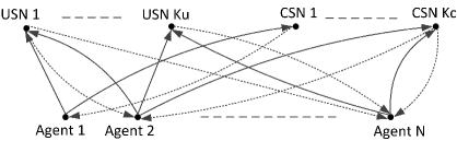
Figure 1: A pictorial representation of the communication graph between system nodes and players. Solid arrows denote the uplink channels and dashed arrows denote the downlink channels.

II-A Game-theoretic Set-up

Consider a non-cooperative game with $N$ players indexed over $\mathcal{N}=\left\{1,\cdots,N\right\}$. Let $x^{i}$ ($i\in\mathcal{N}$), and $\boldsymbol{x}=\left[x^{1},\cdots,x^{N}\right]^{\top}$ denote the action of the $i$th player and the collection of all players’ actions, respectively. The utility function of the $i$th player is denoted by $u_{i}\left(x^{i},\boldsymbol{x}^{-i}\right)$ where $\boldsymbol{x}^{-i}$ is the vector of those other players’ actions that affect the $i$th player’s utility. The utility function of the $i$th player quantifies the desirability of any point in the action space for the $i$th player. The actions of players are limited by $L$ convex constraints denoted by $\boldsymbol{g}\left(\boldsymbol{x}\right)\leq 0$ where $\boldsymbol{g}\left(\cdot\right)=\left[g_{1}\left(\cdot\right),\cdots,g_{L}\left(\cdot\right)\right]^{\top}$ is a mapping from $\mathbb{R}^{N}$ to $\mathbb{R}^{L}$. The set of constraint functions is indexed over $\mathcal{L}=\left\{p\in\mathbb{N}:1\leq p\leq L\right\}$. Let $\mathcal{S}$ denote the action space of players, i.e.,

$$\mathcal{S}=\left\{\boldsymbol{x}\in\mathbb{R}^{N}s.t.\,\boldsymbol{g}\left(\boldsymbol{x}\right)\leq 0\right\}.$$

We assume that $\mathcal{S}$ is a compact and convex subset of $\mathbb{R}^{N}$.

In non-cooperative games, each player is interested in maximizing its own utility function, irrespective of other players. Since the maximizers of utility functions of players do not necessarily coincide with each other, a trade-off is required. In this paper, the Nash equilibrium is considered as the canonical solution concept of the non-cooperative game among players. Let $\boldsymbol{x}_{\rm NE}\in\mathcal{S}$ be the NE of the game among players. Then, at the NE, no player has incentive to unilaterally deviate its action from its NE strategy, i.e.,

$$x^{i}_{\rm NE}=\arg\underset{x^{i}\in\mathcal{S}\left(\boldsymbol{x}^{-i}_{\rm NE,C}\right)}{\max} u_{i}\left(x^{i},\boldsymbol{x}^{-i}_{\rm NE}\right),\forall i\in\mathcal{N},$$

where $\boldsymbol{x}^{-i}_{\rm NE,C}$ is the collection of NE strategies of players which are coupled with the $i$th player through constraints, and $\mathcal{S}\left(\boldsymbol{x}^{-i}_{\rm NE,C}\right)$ is the set of possible actions of the $i$th player given $\boldsymbol{x}^{-i}_{\rm NE,C}$. The vector of all utility functions is denoted by $U\left(\boldsymbol{x}\right)=\left[u_{1}\left(\boldsymbol{x}\right),\cdots,u_{N}\left(\boldsymbol{x}\right)\right]^{\top}$.

Let $\mathcal{F}$ denote the class of functions from $\mathbb{R}^{N}$ to $\mathbb{R}^{N}$ such that any $N$-player non-cooperative game with the constraint set $\mathcal{S}$ and utility function vector in $\mathcal{F}$ admits at least one NE. By the class of non-cooperative games $\mathcal{G}=\langle\mathcal{N},\mathcal{S},\mathcal{F}\rangle$, we mean the set of all games with $N$ players, the action space $\mathcal{S}$, and the utility function vector in $\mathcal{F}$, i.e., $U\left(\cdot\right)\in\mathcal{F}$.

II-B Communication Model

In this paper, we consider a distributed Nash seeking set-up wherein, at each time-step, players communicate with a set of utility system nodes (USNs) and constraint system nodes (CSNs) to obtain the required utility/constraint related information for updating their actions. A USN computes utility-related information for a set of players, e.g., the utility functions of players or their partial derivatives. A CSN evaluates a subset of constraints based on the received actions of players. Each utility function or constraint is evaluated at only one USN or CSN, respectively. The number of USNs and CSNs are denoted by $K_{\rm u}$ and $K_{\rm c}$, respectively, with $K_{\rm u}\leq N$ and $K_{\rm c}\leq L$. We use $\text{USN}_{l}$ ($l\in\left\{1,\dots,K_{\rm u}\right\}$) and $\text{CSN}_{n}$ ($n\in\left\{1,\dots,K_{\rm c}\right\}$) to refer to the $l$th USN and $n$th CSN, respectively.

At each time-step, player $i$ transmits its action to $\text{USN}_{l}$ if its action affects at least a utility function evaluated by $\text{USN}_{l}$. The set of players which transmit their actions to $\text{USN}_{l}$ is denoted by $\mathcal{N}_{{\rm usn}_{l}}$. We use the mapping $\pi\left(\cdot\right)$, from $\left\{1,\cdots,N\right\}$ to $\left\{1,\dots,K_{\rm u}\right\}$, to indicate the USN which computes the utility-related information for a given player, i.e., $\pi\left(i\right)=l$ if $\text{USN}_{l}$ computes the utility-related information for the $i$th player. Thus, the utility-related information for the $i$th player is computed by $\text{USN}_{\pi\left(i\right)}$.

Similarly, at each time-step, player $i$ transmits its action to $\text{CSN}_{n}$ if its action affects at least one constraint function evaluated by $\text{CSN}_{n}$. The set of players which transmit their actions to $\text{CSN}_{n}$ is represented by $\mathcal{N}_{{\rm csn}_{n}}$. We use the mapping $\phi\left(\cdot\right)$, from $\left\{1,\cdots,L\right\}$ to $\left\{1,\dots,K_{\rm c}\right\}$, to indicate the CSN which evaluates a given constraint function, i.e., $\phi\left(p\right)=n$ if $\text{CSN}_{n}$ evaluates the $p$th constraint function. Hence, the $p$th constraint function is evaluated by $\text{CSN}_{\phi\left(p\right)}$. The set of constraint functions which are affected by the $i$th player’s action are denoted by $\mathcal{L}_{i}$.

The communication topology between players and system nodes is given by a bipartite digraph in which the players and the system nodes form two disjoint sets of vertices. There exists a directed edge, in the communication graph, from the $i$th player to $\text{USN}_{l}$ if $i\in\mathcal{N}_{{\rm usn}_{l}}$. Also, there exists a directed edge from $\text{USN}_{\pi\left(i\right)}$ to the $i$th player for all $i\in\mathcal{N}$. Furthermore, there exist a directed edge from the $i$th player to $\text{CSN}_{n}$, and a directed edge from $\text{CSN}_{n}$ to the $i$th player if $i\in\mathcal{N}_{{\rm csn}_{n}}$. We refer to communication channels from players to system nodes as uplink channels and the communications channels between system nodes and players as downlink channels. Fig. 1 shows a pictorial representation of the communication topology between system nodes and players.

Players communicate with system nodes using frequency division multiplexing (FDM) or time division multiplexing (TDM) schemes, i.e., each player broadcasts its action to its neighboring system nodes in the communication graph using a dedicated time or frequency band. Similarly, system nodes communicate with players via FDM or TDM communication schemes. The communication between players and system nodes is performed over noisy communication channels, i.e., players receive noisy information from system nodes, and system nodes receive noisy versions of players’ actions. This will be made more explicit in the next subsection.

$$T^{\star}_{\epsilon,\delta}\left(\mathcal{G},\mathcal{O}\right)=\inf\left\{T\in\mathbb{N}:\exists\mathcal{A}\quad s.t.\sup_{U\left(\cdot\right)\in\mathcal{F}}\inf_{i}\mathsf{Pr}\left(\left\|\boldsymbol{x}_{{\rm NE}_{i},U\left(\cdot\right)}-\mathcal{A}_{T+1}\left({X}_{1:T},{\hat{Y}_{1:T}},\hat{Z}_{1:T}\right)\right\|\geq\epsilon\right)\leq\delta\right\}.$$ (1)

 

II-C Nash Seeking Algorithms

II-C1 The Update Rule

In this paper, we consider a general structure for the Nash seeking algorithms which allows each player’s action to be updated using the past actions of that player as well as the past received utility/constraint related information by that player. Let $\mathcal{A}$ be such a Nash seeking algorithm. Then, under $\mathcal{A}$, the $i$th player’s action at time $k$, i.e., $x^{i}_{k}$, is updated according to the update rule

$$x^{i}_{k}=\mathcal{A}^{i}_{k}\left(X^{i}_{1:k-1},\hat{Y}^{i}_{1:k-1},\hat{Z}^{i}_{1:k-1}\right),$$

where $X^{i}_{1:k-1}$ is the history of the $i$th player’s actions from time $1$ to $k-1$, $\hat{Y}^{i}_{1:k-1}$ denotes the sequence of received utility-related information by the $i$th player from time $1$ to $k-1$, and $\hat{Z}^{i}_{1:k-1}$ denotes the sequence of received constraint-related information by the $i$th player from time $1$ to $k-1$. Here, $\mathcal{A}^{i}_{k}\left(\cdot,\cdot,\cdot\right)$ is a mapping from $\mathbb{R}^{k-1}\times\mathbb{R}^{k-1}\times\mathbb{R}^{\left(k-1\right)\left|\mathcal{L}_{i}\right|}$ to $\mathbb{R}$. Note that $X^{i}_{1:k-1}$, $\hat{Y}^{i}_{1:k-1}$ and $\hat{Z}^{i}_{1:k-1}$ can be written as

$$X^{i}_{1:k-1} =\left\{x^{i}_{t}\right\}_{t=1}^{k-1},$$

$$\hat{Y}^{i}_{1:k-1} =\left\{\hat{y}^{i}_{t}\right\}_{t=1}^{k-1},$$

$$\hat{Z}^{i}_{1:k-1} =\left\{\hat{z}^{i,p}_{t},p\in\mathcal{L}_{i}\right\}_{t=1}^{k-1},$$

, respectively, where $x^{i}_{t}$ is the action of the $i$th player at time $t$, $\hat{y}^{i}_{t}$ denotes the received utility-related information by the $i$th player at time $t$ and $\hat{z}^{i,p}_{t}$ denotes the received information regarding the $p$th constraint by the $i$th player at time $t$.

The $k$th step of the algorithm $\mathcal{A}$ is denoted by

$$\mathcal{A}_{k}\!\!\left(X_{1:k-1},\hat{Y}_{1:k-1},\hat{Z}_{1:k-1}\right)\!\!=\!\!\left\{\!\mathcal{A}^{i}_{k}\!\!\left(X^{i}_{1:k-1},\hat{Y}^{i}_{1:k-1},\hat{Z}^{i}_{1:k-1}\!\!\right)\right\}_{i},$$

where

$$X_{1:k-1} =\left\{x^{i}_{t}:i\in\mathcal{N}\right\}_{t=1}^{k-1},$$

$$\hat{Y}_{1:k-1} =\left\{\hat{y}^{i}_{t}:i\in\mathcal{N}\right\}_{t=1}^{k-1},$$

$$\hat{Z}_{1:k-1} =\left\{\hat{z}^{i,p}_{t}:i\in\mathcal{N},p\in\mathcal{L}_{i}\right\}_{t=1}^{k-1}.$$

We refer to

$$\mathcal{A}=\left\{\mathcal{A}_{k}\left(X_{1:k-1},\hat{Y}_{1:k-1},\hat{Z}_{1:k-1}\right)\right\}_{k},$$

as the Nash seeking algorithm $\mathcal{A}$.

II-C2 Communication and Computation At USNs

The received action of the $i$th player by $\text{USN}_{l}$ at time $k$, i.e., $\hat{x}^{i}_{k,{\rm usn}_{l}}$, can be written as

$$\hat{x}^{i}_{k,{\rm usn}_{l}}=x^{i}_{k}+W^{i}_{k,{\rm usn}_{l}},$$

where $W^{i}_{k,{\rm usn}_{l}}$ is the noise in the uplink channel from the $i$th player to $\text{USN}_{l}$. Let $\hat{X}_{1:k}^{{\rm usn}_{l}}=\left\{\hat{x}^{i}_{t,{\rm usn}_{l}}:i\in\mathcal{N}_{{\rm usn}_{l}}\right\}_{t=1}^{k}$ denote the history of actions received by $\text{USN}_{l}$ from time 1 to time $k$. At time $k$, $\text{USN}_{l}$ computes $y_{k}^{i}$, i.e., the utility-related information for player $i$ at time $k$, for all $i$ such that $\pi\left(i\right)=l$.

In this paper, we study the complexity of solving non-cooperative games under two computation models at USNs. We first consider a general computation model in which $y^{i}_{k}$ is allowed to be any arbitrary function of $u_{i}\left(\cdot\right)$ and the information available at $\text{USN}_{l}$ from time $1$ to $k$, i.e.,

$$y_{k}^{i}=\mathcal{O}_{k,i}\left(\hat{X}_{1:k}^{{\rm usn}_{l}},u_{i}\left(\cdot\right)\right)\quad\forall i:\pi\left(i\right)=l.$$ (2)

where $\mathcal{O}_{k,i}\left(\cdot,\cdot\right)$ is a functional. This formulation allows us to capture the complexity of solving the game class $\mathcal{G}$ under a general class of computation models at USNs in Theorem 1. We refer to $\mathcal{O}=\left\{\mathcal{O}_{k,i}\left(\hat{X}^{{\rm usn}_{\pi\left(i\right)}}_{1:k},u_{i}\left(\cdot\right)\right)\right\}_{k,i}$ as the general computation model at USNs.

We also study the complexity of solving non-cooperative games under the partial-derivative computation model in which $\text{USN}_{l}$ at time $k$ evaluates the partial derivative of the utility function of the $i$th player with respect to its action, i.e., $y^{i}_{k}=\left.\frac{\partial}{\partial\left(x^{i}\right)}u_{i}\left(x^{i},\boldsymbol{x}^{-i}\right)\right|_{\hat{X}^{{\rm usn}_{l}}_{k}}$ for all $i$ with $\pi\left(i\right)=l$. We refer to the partial-derivative computational model for USNs as

$$\mathcal{O}^{1}=\left\{\mathcal{O}^{1}_{k,i}\left(\hat{X}^{{\rm usn}_{\pi\left(i\right)}}_{k},u_{i}\left(\cdot\right)\right)\right\}_{k,i}$$ (3)

where $\hat{X}^{{\rm usn}_{l}}_{k}=\left\{\hat{x}^{i}_{k,{\rm usn}_{l}}:i\in\mathcal{N}_{{\rm usn}_{l}}\right\}$ denotes the set of actions received by $\text{USN}_{l}$ at time $k$ and

$$\mathcal{O}^{1}_{k,i}\left(\hat{X}^{{\rm usn}_{\pi\left(i\right)}}_{k},u_{i}\left(\cdot\right)\right)=\left.\frac{\partial}{\partial\left(x^{i}\right)}u_{i}\left(x^{i},\boldsymbol{x}^{-i}\right)\right|_{\boldsymbol{x}=\hat{X}^{{\rm usn}_{\pi\left(i\right)}}_{k}}.$$

Then, $\text{USN}_{l}$ transmits $y_{k}^{i}$ to the $i$th player for all $i$ with $\pi\left(i\right)=l$. The received utility-related information by the $i$th player at time $k$ can be written as

$$\hat{y}^{i}_{k}=y^{i}_{k}+V^{i}_{k},$$

where $V^{i}_{k}$ is the noise in the downlink channel from the $\text{USN}_{\pi\left(i\right)}$ to the $i$th player.

II-C3 Communication and Computation At CSNs

The received action of the $i$th player by $\text{CSN}_{n}$ at time $k$, i.e, $\hat{x}^{i}_{k,{\rm csn}_{n}}$, can be written as

$$\hat{x}^{i}_{k,{\rm csn}_{n}}=x^{i}_{k}+W^{i}_{k,{\rm csn}_{n}},$$

where $W^{i}_{k,{\rm csn}_{n}}$ is the noise in the uplink channel from the $i$th player to $\text{CSN}_{n}$. The collection of received actions at time $k$ by the $\text{CSN}_{n}$ is denoted by $\hat{X}^{{\rm csn}_{n}}_{k}=\left\{\hat{x}^{i}_{k,{\rm csn}_{n}}:i\in\mathcal{N}_{{\rm csn}_{n}}\right\}$. At time $k$, $\text{CSN}_{n}$ evaluates its associated constraint functions using the received actions at time $k$, i.e.,

$$z^{p}_{k}=g_{p}\left(\hat{X}_{k}^{{\rm csn}_{n}}\right),\quad\forall p:\phi\left(p\right)=n$$

Finally, $\text{CSN}_{n}$ broadcasts $z^{p}_{k}$ to the players which their actions affect $g_{p}\left(\cdot\right)$. If the action of the $i$th player affects the $p$th constraint, the $i$th player will receive

$$\hat{z}^{i,p}_{k}=z^{p}_{k}+V^{i,p}_{k},$$

at time $k$ where $V^{i,p}_{k}$ is the noise in the downlink channel from $\text{CSN}_{\phi\left(p\right)}$ to the player $i$.

Remark 1

Although, we assume that the $\text{CSN}_{n}$ at time $k$ transmits $g_{p}\left(\hat{X}_{k}^{{\rm csn}_{n}}\right)$ to the $i$th player (if $p\in\mathcal{L}_{i}$), our results continue to hold when other computation models are implemented at the CSNs, e.g., when the $\text{CSN}_{n}$ at time $k$ transmits $\left.\frac{\partial}{\partial x^{i}}g_{p}\left(\boldsymbol{x}\right)\right|_{\boldsymbol{x}=\hat{X}_{k}^{{\rm csn}_{n}}}$ to the $i$th player.

TABLE I: Table of the main variables

Variable	Description
$\mathcal{N}$	The set of players
$\mathcal{L}$	The set of constraints
$\mathcal{L}_{i}$	The set of constraints which are affected by the $i$th player action
$\text{USN}_{\pi\left(i\right)}$	The USN which computes utility-related information for the $i$th player
$\text{CSN}_{\phi\left(p\right)}$	The CSN which evaluates the $p$th constraint
$\mathcal{N}_{{\rm usn}_{l}}$	The set of players which transmit their actions to $\text{USN}_{l}$
$\mathcal{N}_{{\rm csn}_{n}}$	The set of players which transmit their actions to $\text{CSN}_{n}$
$x^{i}_{k}$	Action of the $i$th player at time $k$
$X^{i}_{1:k}$	Actions of the $i$th player from time $1$ to $k$
$X_{1:k}$	Actions of all the players from time $1$ to $k$
$\hat{x}^{i}_{k,{\rm usn}_{l}}$	The received action of the $i$th player by $\text{USN}_{l}$ at time $k$
$\hat{X}^{{\rm usn}_{l}}_{k}$	The collection of received actions by $\text{USN}_{l}$ at time $k$
$\hat{X}^{{\rm usn}_{l}}_{1:k}$	The collection of received actions by $\text{USN}_{l}$ from time 1 to $k$
$y^{i}_{k}$	The utility-related information computed by $\text{USN}_{\pi\left(i\right)}$ for the $i$th player
$\hat{y}^{i}_{k}$	The received utility-related information by the $i$th player
$\hat{Y}^{i}_{1:k}$	The history of received utility-related information by the $i$th players from time $1$ to $k$
$\hat{Y}_{1:k}$	The history of received utility-related information by all the players from time $1$ to $k$
$\hat{x}^{i}_{k,{\rm csn}_{n}}$	The received action of the $i$th player by $\text{CSN}_{n}$ at time $k$
$\hat{X}^{{\rm csn}_{n}}_{k}$	The collection of received actions by $\text{CSN}_{n}$ at time $k$
$z^{p}_{k}$	The value of the $p$th constraint at time $k$ evaluated by $\text{CSN}_{\phi\left(p\right)}$
$\hat{z}^{i,p}_{k}$	The received value of the $p$th constraint at time $k$ by the $i$th player
$\hat{Z}^{i}_{1:k}$	The history of received constraint-related information by the $i$th players from time $1$ to $k$
$\hat{Z}_{1:k}$	The history of received constraint-related information by all the players from time $1$ to $k$
$W^{i}_{k,{\rm usn}_{l}}$	The additive noise in the uplink channel from the $i$th player to $\text{USN}_{l}$ at time $k$ ($i\in\mathcal{N}_{{\rm usn}_{l}}$)
$W^{i}_{k,{\rm csn}_{n}}$	The additive noise in the uplink channel from the $i$th player to $\text{CSN}_{n}$ at time $k$ ($i\in\mathcal{N}_{{\rm csn}_{n}}$)
$V^{i}_{k}$	The additive noise in the downlink channel from $\text{USN}_{\pi\left(i\right)}$ to the $i$th player at time $k$
$V^{i,p}_{k}$	The additive noise in the downlink channel which transmits $z^{p}_{k}$ to the $i$th player at time $k$ ($p\in\mathcal{L}_{i}$)

II-D The Complexity Criterion

Consider the class of games $\mathcal{G}$ and and the computation model $\mathcal{O}$. Then, the $\left(\epsilon,\delta\right)$-complexity of solving the class of games $\mathcal{G}$ with the computation model $\mathcal{O}$, denoted by $T^{\star}_{\epsilon,\delta}\left(\mathcal{G},\mathcal{O}\right)$, is defined in (1) where $\boldsymbol{x}_{{\rm NE}_{i},U\left(\cdot\right)}$ is a NE of the non-cooperative game with the utility function vector given by $U\left(\boldsymbol{\cdot}\right)\in\mathcal{F}$. According to (1), the $\left(\epsilon,\delta\right)$-complexity of solving the class of games $\mathcal{G}$ with the computation model $\mathcal{O}$ is defined as the smallest positive integer $T$ for which there exists an algorithm $\mathcal{A}$ such that, for any game in $\mathcal{G}$, the probability of $\epsilon$ deviation of the algorithm’s output at time $T+1$ from at least a NE of the game is less than $\delta$. Note that (1) assigns a positive integer to any class of games. For a given pair of $\left(\mathcal{G},\mathcal{O}\right)$, a small value of $T^{\star}_{\epsilon,\delta}\left(\mathcal{G},\mathcal{O}\right)$ indicates that the class of games $\mathcal{G}$ with the computation model $\mathcal{O}$ can be solved faster compared to a large value of $T^{\star}_{\epsilon,\delta}\left(\mathcal{G},\mathcal{O}\right)$. The complexity of solving the game class $\mathcal{G}$ under the computation model $\mathcal{O}^{1}$ can be defined in a similar way.

Remark 2

The $\epsilon$-Nash equilibrium ($\epsilon$-NE) is a closely related solution concept to the NE which is defined as the point such that no play can gain more than $\epsilon$ by unilaterally deviating its strategy from its $\epsilon$-NE strategy. However, an $\epsilon$-NE is not always close to a NE since game-theoretic problems are not necessarily convex problems and a NE is not necessarily the maximizer/minimizer of utility functions of all players [12]. Hence, we do not consider $\epsilon$-NE as a solution concept in this paper.

II-E Modeling Assumptions

In this paper, we impose the following assumptions on the Nash seeking algorithms and the noise terms in the uplink/downlink communication channels:

1. $X_{1}$ is specified by the algorithm $\mathcal{A}$, and the algorithm $\mathcal{A}$ uses the same value of $X_{1}$ for solving any game.

2. $\left\{W^{i}_{k,{\rm usn}_{l}},i\in\mathcal{N}_{{\rm usn}_{l}}\right\}_{k}$ is a collection of zero mean, independent and identically distributed (i.i.d.) random variables with variance $\sigma^{2}_{{\rm usn}_{l}}>0$ for all $1\leq l\leq K_{\rm u}$.

3. $\left\{W^{i}_{k,{\rm csn}_{n}},i\in\mathcal{N}_{{\rm csn}_{n}}\right\}_{k}$ is a collection of zero mean, i.i.d. random variables with variance $\sigma^{2}_{{\rm csn}_{n}}>0$ for all $1\leq n\leq K_{\rm c}$.

4. $\left\{V^{i}_{k},V^{i,p}_{k},p\in\mathcal{L}_{i}\right\}_{k}$ is a collection of i.i.d. random variables with zero mean and variance $\sigma^{2}_{i}>0$ for all $i\in\mathcal{N}$.

5. All the uplink/downlink noise terms are jointly independent.

II-F Organization of The Paper and Notations

The rest of this paper is organized as follows. Section III states our main results on the complexity of solving two classes of non-cooperative games. Section IV presents the derivation of our results, and Section V concludes the paper.

In the rest of this paper, we use the following notations from asymptotic analysis literature. For two positive functions $f\left(x\right)$ and $g\left(x\right)$, we say $f\left(x\right)=\Omega\left(g\left(x\right)\right)$ if $\lim\inf_{x\downarrow 0}\frac{f\left(x\right)}{g\left(x\right)}>0$. We also say $f\left(x\right)=\Theta\left(g\left(x\right)\right)$ if $\lim\inf_{x\downarrow 0}\frac{f\left(x\right)}{g\left(x\right)}>0$ and $\lim\sup_{x\downarrow 0}\frac{f\left(x\right)}{g\left(x\right)}<\infty$. Our main notations are summarized in Table I.

III Results and Discussions

In this section, we establish various lower bounds on the complexity of solving two game classes under different assumptions on the distribution of uplink/downlink noise terms and different computation models at USNs. In Subsection III-A, we derive two lower bounds on the complexity of solving the game class $\mathcal{G}$ under the general computation model at USNs without assuming any particular distribution for the uplink/downlink noise terms. In Subsection III-B, we establish a lower bound on the complexity of solving a subclass of $\mathcal{G}$, denoted by $\mathcal{G}_{\gamma}$, under Gaussian uplink/downlink channels and the partial-derivative computation model. Subsection III-B presents a lower bound on the complexity of solving the game class $\mathcal{G}_{\gamma}$ under noiseless uplink channels, non-Gaussian downlink channels, and the partial-derivative computation model. Subsection III-D discusses the complexity of solving the game class $\mathcal{G}_{\gamma}$ under the partial-derivative computation model when both uplink and downlink channels are non-Gaussian distributed.

III-A General Computation model at USNs and General Uplink/Downlink Channels

In this subsection, we study the computational complexity of solving the game class $\mathcal{G}$ without imposing any particular structure on the computation model at the USNs, or imposing any specific probability distribution on the noise in the uplink/downlink channels. To this end, we first give the definition of the total capacity of downlink channels, the notion of $2\epsilon$-distinguishable subsets of $\mathcal{S}$, and the Kolmogorov capacity of $\mathcal{S}$.

The total capacity of downlink channels from USNs to players is defined as

$$C_{\rm down}=\max_{p_{Y}\left(\boldsymbol{y}\right),\mathsf{E}\left[\left\|Y\right\|^{2}\right]\leq\alpha}\mathsf{I}\left[y^{1},\cdots,y^{N};\hat{y}^{1},\cdots,\hat{y}^{N}\right]$$

where $y^{i}$ and $\hat{y}^{i}$ are the input and the output of the downlink channel from $\text{USN}_{\pi\left(i\right)}$ to the $i$th player, respectively, $Y=\left[y^{1},\cdots,y^{N}\right]^{\top}$, $p_{Y}\left(\boldsymbol{y}\right)$ is the joint distribution of $Y$, and $\alpha$ is the total average power constraint of the downlink channels between USNs and players.

Definition 1

A subset of $\mathcal{S}$ is $2\epsilon$-distinguishable if the distance between any two of its points is more than $2\epsilon$ [13].

Definition 2

Let $\mathcal{M}_{2\epsilon}\left(\mathcal{S}\right)$ denote the cardinality of maximal size $2\epsilon$ distinguishable subsets of $\mathcal{S}$. Then, the Kolmogorov capacity of $\mathcal{S}$ is defined as $\log\mathcal{M}_{2\epsilon}\left(\mathcal{S}\right)$ [13].

The next theorem establishes a lower bound on $T^{\star}_{\epsilon,\delta}\left(\mathcal{G},\mathcal{O}\right)$.

Theorem 1

Let $T^{\star}_{\epsilon,\delta}\left(\mathcal{G},\mathcal{O}\right)$ denote the complexity of the class of $N$-player non-cooperative games $\mathcal{G}$ with the continuous action space $\mathcal{S}$. Then, we have

$$T^{\star}_{\epsilon,\delta}\left(\mathcal{G},\mathcal{O}\right)\geq\frac{\left(1-\delta\right)\log\mathcal{M}_{2\epsilon}\left(\mathcal{S}\right)-1}{C_{\rm down}}$$ (4)

where $C_{\rm down}$ is the total capacity downlink channels from USNs to players, and $\log\mathcal{M}_{2\epsilon}\left(\mathcal{S}\right)$ is the Kolmogorov $2\epsilon$-capacity of the action space $\mathcal{S}$.

Proof:

See Subsection IV-A. ∎

Theorem 1 establishes an algorithm-independent lower bound on the order of complexity of solving the game class $\mathcal{G}$. According to this theorem, $T^{\star}_{\epsilon,\delta}\left(\mathcal{G},\mathcal{O}\right)$ is lower bounded by the ratio of the Kolmogorov $2\epsilon$-capacity of the action space $\mathcal{S}$ to the total Shannon capacity of the downlink channels. Note that the Kolmogorov $2\epsilon$-capacity of $\mathcal{S}$ can be interpreted as a measure of players’ ambiguity about their NE strategies. Thus, as $\log\mathcal{M}_{2\epsilon}\left(\mathcal{S}\right)$ becomes large, $T^{\star}_{\epsilon,\delta}\left(\mathcal{G},\mathcal{O}\right)$ is expected to increase since players have to search in a bigger space to find their NE strategies. Based on Theorem 1, $C_{\rm down}$ has a reverse impact on $T^{\star}_{\epsilon,\delta}\left(\mathcal{G},\mathcal{O}\right)$. Note that $C_{\rm down}$ is an indication of the information transmission quality from USNs to players. That is, as $C_{\rm down}$ decreases, players will receive noisier information regarding their utility functions compared with a large value of $C_{\rm down}$.

Theorem 1 depends on the $2\epsilon$-capacity of the constraint set $\mathcal{S}$ which is usually hard to compute unless the action space of players is restricted to special geometries. As $\mathcal{M}_{2\epsilon}\left(\mathcal{S}\right)$ is just the maximum number of $\epsilon$-balls that can be packed into $\mathcal{S}$, it is asymptotically equal to $\frac{{\rm Vol}\left(\mathcal{S}\right)}{{\rm Vol}\left(B_{\epsilon}\right)}=\frac{{\rm Vol}\left(\mathcal{S}\right)}{\alpha_{N}\epsilon^{N}}$ as $\epsilon$ tends to zero, where $B_{\epsilon}$ is the $N$-ball of radius $\epsilon$, and $\alpha_{N}$ is the $N$-dimensional spherical constant under the assumed norm. Thus, the complexity is at least of order $\log\frac{1}{\epsilon}$ as $\epsilon$ becomes small. The next result establishes a non-asymptotic lower bound of the same order, by lower bounding $\mathcal{M}_{2\epsilon}\left(\mathcal{S}\right)$ using a result from lattice theory.

Corollary 1

The complexity of solving the class of $N$-player non-cooperative games $\mathcal{G}$ with continuous action space $\mathcal{S}$ can be bower bounded as

$$T^{\star}_{\epsilon,\delta}\left(\mathcal{G},\mathcal{O}\right)\geq\frac{\left(1-\delta\right)\!\!\left(N\log\frac{1}{2\epsilon}\!+\!\log\left({\rm Vol}\left(\mathcal{S}\right)\!-\!\epsilon{\rm P}\left(\mathcal{S}\right)\right)\right)-1}{C_{\rm down}}$$ (5)

where ${\rm Vol}\left(\mathcal{S}\right)$ and ${\rm P}\left(\mathcal{S}\right)$ are the volume and the surface area of the action space of players, respectively.

Proof:

See Subsection IV-B. ∎

Based on Corollary 1, the lower bound on $T^{\star}_{\epsilon,\delta}\left(\mathcal{G},\mathcal{O}\right)$ increases at least linearly with the number of players. This is due to the fact that the amount of uncertainty about the NE increases as the number of players becomes large. Recall that $\log\mathcal{M}_{2\epsilon}\left(\mathcal{S}\right)$ is a quantitative indicator of ambiguity about the NE. Furthermore, $\epsilon$ has a logarithmic effect on $T^{\star}_{\epsilon,\delta}\left(\mathcal{G},\mathcal{O}\right)$, i.e., the complexity of solving the class of games $\mathcal{G}$ increases according to $\Omega\left(\log\frac{1}{\epsilon}\right)$ as $\epsilon$ becomes small. Hence, based on Corollary 1, the game class $\mathcal{G}$ cannot be solved faster than $\Theta\left(\log\frac{1}{\epsilon}\right)$ time-steps regardless of uplink/downlink noise distributions, and the computation model at the USNs.

According to Corollary 1, the lower bound on the complexity of solving the game class $\mathcal{G}$ increases as the volume of the action space of players becomes large. Also, for a given surface area of action space of players, i.e., ${\rm P}\left(\mathcal{S}\right)$, the volume of action space of players can be upper bounded using the isoperimetric inequality for convex bodies [14] as follows:

$${\rm Vol}\left(\mathcal{S}\right)\leq\frac{{\rm Vol}\left(\rm B\right)}{\left({\rm P}\left(\rm B\right)\right)^{\frac{N}{N-1}}}{\rm P}\left(\mathcal{S}\right)^{\frac{N}{N-1}}$$ (6)

where $\rm B$ is the closed unit ball in $N$-dimensional Euclidean space $\mathbb{R}^{N}$. Note that the equality in (6) is achieved if and only if $\mathcal{S}$ is a ball in $\mathbb{R}^{N}$[14]. Thus, for a given surface area of action space of players ${\rm P}\left(\mathcal{S}\right)$, the lower bound on the complexity of solving games in the class $\mathcal{G}$ increases as the action space of players becomes closer to a ball in $\mathbb{R}^{N}$ with the volume $\frac{{\rm Vol}\left(\rm B\right)}{\left({\rm P}\left(\rm B\right)\right)^{\frac{N}{N-1}}}{\rm P}\left(\mathcal{S}\right)^{\frac{N}{N-1}}$.

III-B Partial-derivative Computation Model at USNs and Gaussian Uplink/Downlink Channels

In this section, we establish a lower bound on the complexity of solving a subclass of $\mathcal{G}$, denoted by $\mathcal{G}_{\gamma}$, under the partial-derivative computation model (see equation (3)) when the communication noise in the uplink and downlink channels is Gaussian distributed. We also compare the complexity of solving the game class $\mathcal{G}_{\gamma}$ with the complexity of solving the class of strongly convex optimization problems. To specify the game class $\mathcal{G}_{\gamma}$, we first define the notion of pseudo-gradient for a utility function vector as follows.

Definition 3

The pseudo-gradient of the utility function vector $U\left(\boldsymbol{x}\right)=\left[u_{1}\left(x^{1},\boldsymbol{x}^{-1}\right),\cdots,u_{N}\left(x^{N},\boldsymbol{x}^{-N}\right)\right]^{\top}$ is defined as

$$\tilde{\nabla}U\left(\boldsymbol{x}\right)\!\!=\!\!\left[\frac{\partial}{\partial\left(x^{1}\right)}u_{1}\left(x^{1},\boldsymbol{x}^{-1}\right),\cdots,\frac{\partial}{\partial\left(x^{N}\right)}u_{N}\left(x^{N},\boldsymbol{x}^{-N}\right)\right]^{\top}$$

We use $J_{\tilde{\nabla}U}\left(\boldsymbol{x}\right)$ to denote the Jacobian matrix of the vector valued function $\tilde{\nabla}U\left(\boldsymbol{x}\right)$, i.e.,

$$\left[J_{\tilde{\nabla}U}\left(\boldsymbol{x}\right)\right]_{ij}=\frac{\partial^{2}}{\partial\left(x^{j}\right)\left(x^{i}\right)}u_{i}\left(x^{i},\boldsymbol{x}^{-i}\right),\quad 1\leq i,j\leq N$$

We next specify a set of utility vector functions, denoted by $\mathcal{F}_{\gamma}$, which is used to define the game class $\mathcal{G}_{\gamma}$.

Definition 4

The set of utility vector functions $\mathcal{F}_{\gamma}$ is defined as the set of all vector valued functions $U\left(\boldsymbol{x}\right)$ from $\mathbb{R}^{N}$ to $\mathbb{R}^{N}$ such that

1. The $N$-player non-cooperative game with utility vector function given by $U\left(\boldsymbol{x}\right)$ and the constraint set $\mathcal{S}$ admits at least a Nash equilibrium (NE).

2. The matrix $J_{\tilde{\nabla}U}\left(\boldsymbol{x}\right)$ exists for all $\boldsymbol{x}$ in $\mathcal{S}$.

3. The matrix $J_{\tilde{\nabla}U}\left(\boldsymbol{x}\right)$ satisfies $\left\|J_{\tilde{\nabla}U\left(\boldsymbol{x}\right)}\right\|\geq\gamma>0$ for all $\boldsymbol{x}\in\mathcal{S}$ where $\left\|J_{\tilde{\nabla}U}\left(\boldsymbol{x}\right)\right\|$ denotes the matrix norm of $J_{\tilde{\nabla}_{U}}\left(\boldsymbol{x}\right)$.

The next definition specifies the game class $\mathcal{G}_{\gamma}$.

Definition 5

The class of games $\mathcal{G}_{\gamma}=\langle\mathcal{N},\mathcal{S},\mathcal{F}_{\gamma}\rangle$ is defined as the set of all non-cooperative games with $N$ players, the constraint set $\mathcal{S}$, and the utility function vector $U\left(\cdot\right)$ in $\mathcal{F}_{\gamma}$.

Note that the game class $\mathcal{G}_{\gamma}$ reduces to the class $\mathcal{G}$ when $\gamma$ is equal to zero. The complexity of solving the game class $\mathcal{G}_{\gamma}$ heavily depends on $J_{\tilde{\nabla}U}\left(\boldsymbol{x}\right)$ as shown in Theorem 2.

Remark 3

We note that both $\tilde{\nabla}U\left(\boldsymbol{x}\right)$ and $J_{\tilde{\nabla}U}\left(\boldsymbol{x}\right)$ play important roles in the game theory and system theory literature. To clarify this point, consider an unconstrained $N$-player game with the utility vector function $U\left(\boldsymbol{x}\right)=\left[u_{i}\left(x^{i},\boldsymbol{x}^{-i}\right)\right]_{i}$ such that each $u_{i}\left(x^{i},\boldsymbol{x}^{-i}\right)$ is concave in $x^{i}$. Then, any solution of $\tilde{\nabla}_{U}\left(\boldsymbol{x}\right)=\boldsymbol{0}$ will be a NE of this game. Also, consider the dynamical system $\dot{\boldsymbol{x}}=\tilde{\nabla}U\left(\boldsymbol{x}\right)$. Then, any NE of the aforementioned game will be an equilibrium of this dynamical system and the eigenvalues of the matrix $J_{\tilde{\nabla}U}\left(\boldsymbol{x}\right)$ determine the local stability of this dynamical system around its equilibria. Moreover, the matrix $J_{\tilde{\nabla}U}\left(\boldsymbol{x}\right)$ can be used to study the uniqueness of the NE in non-cooperative games [15].

The next theorem studies the complexity of solving the game class $\mathcal{G}_{\gamma}$ under the partial-derivative computation model and Gaussian distributed uplink/downlink channels. In the derivation of Theorem 2, it is assumed that the constraint set $\mathcal{S}$ contains a 2-ball with radius $\sqrt{2}\epsilon$, i.e., the set of all points in a 2-dimensional plane with the distance $\sqrt{2}\epsilon$ from a point in $\mathcal{S}$.

Theorem 2

Let $T^{\star}_{\epsilon,\delta}\left(\mathcal{G}_{\gamma},\mathcal{O}^{1}\right)$ denote the complexity of solving the game class $\mathcal{G}_{\gamma}$ under the partial-derivative computation model at USNs. Then, for Gaussian distributed uplink/downlink channels and $\delta\leq 0.5$, we have

$$T^{\star}_{\epsilon,\delta}\left(\mathcal{G}_{\gamma},\mathcal{O}^{1}\right)\geq\frac{\left(2\left(1-\delta\right)-1\right)\min_{i}\sigma^{2}_{i}}{4\gamma^{2}\epsilon^{2}},$$ (7)

where $\sigma_{i}^{2}$ is the variance of noise at the player $i$’s receiver.

Proof:

See Subsection IV-C. ∎

Theorem 2 establishes an algorithm-independent lower bound on the complexity of solving the game class $\mathcal{G}_{\gamma}$. According to this result, the game class $\mathcal{G}_{\gamma}$ cannot be solved faster than $\Theta\left(\frac{1}{\gamma^{2}\epsilon^{2}}\right)$ under the partial-derivative computation model and Gaussian noise model for uplink and downlink channels.

It is helpful to compare the complexity of solving the game class $\mathcal{G}_{\gamma}$ with that of solving a black-box convex optimization problem. The complexity of solving black-box optimization problems is studied under an oracle-based setting in which optimization algorithms rely on an oracle for function evaluation. In this setting, the oracle receives noise-free queries from the optimization algorithm, and, the algorithm receives a noisy version of oracle’s response [6]. The next corollary studies the complexity of solving the game class $\mathcal{G}_{\gamma}$ in a similar setting, i.e., under noiseless uplink channels and Gaussian downlink channels.

Corollary 2

Let $T^{\star}_{\epsilon,\delta}\left(\mathcal{G}_{\gamma},\mathcal{O}^{1}\right)$ denote the complexity of solving the class $\mathcal{G}_{\gamma}$ using the partial-derivative computation model. Then, for noiseless uplink channels, Gaussian distributed downlink channels and $\delta\leq 0.5$, we have

$$T^{\star}_{\epsilon,\delta}\left(\mathcal{G}_{\gamma},\mathcal{O}^{1}\right)\geq\frac{\left(2\left(1-\delta\right)-1\right)\min_{i}\sigma^{2}_{i}}{4\gamma^{2}\epsilon^{2}}.$$

Proof:

The proof is similar to that of Theorem 2 and is skipped. ∎

Next, we use Corollary 2 to compare the complexity of solving the class $\mathcal{G}_{\gamma}$ with the complexity of solving a class of convex optimization problems using the oracle-based setting. To this end, consider the following optimization problem

$$\underset{\boldsymbol{x}\in\mathcal{S}}{\min} f\left(\boldsymbol{x}\right),$$

where $\mathcal{S}$ is a convex set, and $f\left(\boldsymbol{x}\right)$ belongs to the class of continuous and strongly convex functions $\mathcal{F}_{\rm sc}$. The complexity of solving the class of convex optimization problems with the objective function in $\mathcal{F}_{\rm sc}$ is defined as [6]

$$\inf\left\{T\in\mathbb{N}:\exists\mathcal{A}\quad s.t.\sup_{f\left(\cdot\right)\in\mathcal{F}_{\rm sc}}\mathsf{Pr}\left(f\left(\boldsymbol{x}_{T+1}\right)-f^{\star}\geq\epsilon\right)\leq\delta\right\}$$

where $\boldsymbol{x}_{T+1}$ is the output of the algorithm $\mathcal{A}$ after $T$ queries, and $f^{\star}=\inf_{\boldsymbol{x}\in\mathcal{S}}f\left(\boldsymbol{x}\right)$. It is shown in [6] that the complexity of solving the class of strictly convex optimization problems under the subgradient computation model and Gaussian noise model is given by $\Omega\left(\frac{1}{\epsilon}\right)$. According to the Corollary 2, the game class $\mathcal{G}_{\gamma}$ is harder to solve compared with the class of strictly convex optimization problems since the games are non-convex problems, and NE is more sophisticated solution concept compared with the minimizer of a convex function (see Remark 2 for more details).

III-C Partial-derivative Computation Model at USNs, Non-Gaussian Downlink Channels and Noiseless Uplink Channels

In this subsection, we study the complexity of solving the game class $\mathcal{G}_{\gamma}$ under the partial-derivative computation model when the downlink channels are not necessarily Gaussian and the uplink channels are noiseless. To this end, let $p_{V^{i}}\left(x\right)$ denote the common probability distribution function (PDF) of the collection of random variables $\left\{V^{i}_{k}\right\}_{k}$, i.e., the collection of noise terms in the downlink channel from ${\rm USN}_{\pi\left(i\right)}$ to player $i$. To investigate the complexity of the game class $\mathcal{G}_{\gamma}$ in the non-Gaussian setting, we assume that $p_{V^{i}}\left(x\right)$ satisfies the following mild assumptions for all $1\leq i\leq N$

1. The PDF $p_{V^{i}}\left(x\right)$ is non-zero everywhere on $\mathbb{R}$.

2. The PDF $p_{V^{i}}\left(x\right)$ is at least 3 times continuously differentiable, i.e., $p_{V^{i}}\left(x\right)\in C^{3}$.

3. There exist positive constants $\beta_{1},\beta_{2},\beta_{3}>0$ such that

   $$\left|\frac{d^{3}}{dx^{3}}\log p_{V^{i}}\left(x\right)\right|\leq\beta_{1}+\beta_{2}\left|x\right|^{\beta_{3}}\quad\forall x\in\mathbb{R}$$

4. The tail of the random variable $\left|V^{i}_{k}\right|$ decays faster than $x^{-\left(\beta_{3}+1\right)}$, i.e., we have

   $$\lim_{x\rightarrow\infty}x^{\left(\beta_{3}+1+r\right)}\mathsf{Pr}\left\{\left|V^{i}_{k}\right|\geq x\right\}=0\quad\forall k$$

   for some $r>0$.

The next theorem derives a lower bound on the complexity of solving the game class $\mathcal{G}_{\gamma}$ in the non-Gaussian setting.

Theorem 3

Let $T^{\star}_{\epsilon,\delta}\left(\mathcal{G}_{\gamma},\mathcal{O}^{1}\right)$ denote the complexity of solving the $N$-player non-cooperative games in the class $\mathcal{G}_{\gamma}$ using the partial-derivative computation model at USNs. Assume that the PDFs of the downlink noise terms satisfy the assumptions 1-4 above and the uplink channels are noiseless. Then, for $\delta\leq 0.5$ we have

$$T^{\star}_{\epsilon,\delta}\left(\mathcal{G}_{\gamma},\mathcal{O}^{1}\right)\geq\frac{2\left(1-\delta\right)-1}{4N\epsilon^{2}\gamma^{2}\max_{i}\mathcal{I}_{i}+O\left(\epsilon^{3}\right)}.$$

where $\mathcal{I}_{i}$ is the Fisher information of the PDF $p_{V^{i}}\left(x\right)$ with respect to a shift parameter.

Proof:

See Subsection IV-D. ∎

Theorem 3 establishes a lower bound on the complexity of solving the game class $\mathcal{G}_{\gamma}$ under noiseless uplink channels and non-Gaussian downlink channels. In Corollary 2, we showed that the complexity of solving the game class $\mathcal{G}_{\gamma}$ under the partial-derivative computation model is at least of the order ${\frac{1}{\gamma^{2}\epsilon^{2}}}$, as $\epsilon$ becomes small, when the uplink channels are noiseless and the downlink channels are Gaussian distributed. According to Theorem 3, the lower bound on the complexity of solving the game class $\mathcal{G}_{\gamma}$ is also of the order $\frac{1}{\gamma^{2}\epsilon^{2}}$ when the uplink channels are noiseless and the downlink channels are not necessarily Gaussian distributed.

Theorem 3 is established by deriving an asymptotic expansion for the Kullback-Leibler (KL) distance between the PDF $p_{V^{i}}\left(x\right)$ and its shifted version. More precisely, we show that

$$\mathsf{D}\left[p_{V^{i}}\left(x\right)\left\|p_{A_{i}\boldsymbol{\tau}+V^{i}}\left(x\right)\right.\right]=\frac{1}{2}\mathcal{I}_{i}\left(A_{i}\boldsymbol{\tau}\right)^{2}+O\left(\left\|\boldsymbol{\tau}\right\|^{3}\right)$$

where $A_{i}$ is a 1-by-$N$ row vector, $\boldsymbol{\tau}$ is an $N$-by-1 column vector, $p_{A_{i}\boldsymbol{\tau}+V^{i}}\left(x\right)$ is the PDF of $A_{i}\boldsymbol{\tau}+V^{i}$, and $\mathcal{I}_{i}$ is the Fisher information of $p_{V^{i}}\left(x\right)$ with respect to a shift parameter. Since the Taylor series of a real function is not necessarily convergent, Theorem 3 is proved using Taylor expansion Theorem. The assumptions 1-4 above are used to bound the remainder integral which appears in the Taylor expansion (see Lemma 6 in Subsection IV-D and its proof for more details).

III-D Partial-derivative Computation Model at USNs With Arbitrarily Distributed Uplink and Downlink Channels

The next theorem establishes a lower bound on the complexity of solving the game class $\mathcal{G}_{\gamma}$ under the partial-derivative computation model when the uplink and downlink channels are not necessarily Gaussian distributed.

Theorem 4

The complexity of solving the game class $\mathcal{G}_{\gamma}$ using the partial-derivative computation model at USNs is lower bounded by

$$T^{\star}_{\epsilon,\delta}\left(\mathcal{G}_{\gamma},\mathcal{O}^{1}\right)\geq\sup_{A:\left\|A\right\|\geq\gamma,{\mathcal{S}}_{2\epsilon}\in\mathcal{S}}\frac{\left(1-\delta\right)\log\left|{\mathcal{S}}_{2\epsilon}\right|-1}{\mathsf{I}\left[\boldsymbol{x}^{\star}_{M};-A\boldsymbol{x}^{\star}_{M}+\hat{W}_{A}\right]}$$ (8)

where ${\mathcal{S}}_{2\epsilon}$ is a $2\epsilon$-distinguishable subset of $\mathcal{S}$, $A=\left[a_{ij}\right]$ is an $N$-by-$N$ symmetric, negative definite matrix, $\boldsymbol{x}^{\star}_{M}$ is a random vector taking value in ${\mathcal{S}}_{2\epsilon}$ with uniform distribution, the random vector $\hat{W}_{A}=\left[\hat{W}^{i}_{1}\right]_{i=1}^{N}$ is defined as

$$\hat{W}^{i}_{1}=\left(\sum_{j\in\mathcal{N}_{{\rm usn}_{\pi\left(i\right)}}}a_{ij}W^{j}_{1,{\rm usn}_{\pi\left(i\right)}}\right)+V^{i}_{1},\quad 1\leq i\leq N$$

and $\mathsf{I}\left[\boldsymbol{x}^{\star}_{M};-A\boldsymbol{x}^{\star}_{M}+\hat{W}_{A}\right]$ is the mutual information between $\boldsymbol{x}^{\star}_{M}$ and $-A\boldsymbol{x}^{\star}_{M}+\hat{W}_{A}$.

Proof:

See Subsection 4. ∎

Theorem 8 derives a lower bound on the complexity of solving the game class $\mathcal{G}_{\gamma}$ which depends on the constraint set $\mathcal{S}$, the constant $\gamma$ and the noise distribution in the uplink and downlink channels. The optimization in (8) is over the set of all symmetric, negative definite matrices with norm greater than or equal to $\gamma$, and the set of all $2\epsilon$-distinguishable subsets of $\mathcal{S}$. The matrix $A$ in (8) stems from the construction of quadratic utility functions in the proof of Theorem 4, the set $\mathcal{S}_{2\epsilon}$ and the matrix $A$ jointly represent a finite subset of the function class $\mathcal{F}_{\gamma}$, and $\hat{W}^{i}_{1}$ represents the combined impact of uplink and downlink channels at player $i$’s receiver under the constructed quadratic utility functions (see the proof of this theorem for more details).

Theorem 4 can be used to numerically obtain a lower bound on the complexity of solving the game class $\mathcal{G}_{\gamma}$ up to $\epsilon$ accuracy when the uplink/downlink channels are not Gaussian distributed. Note that according to (8), $T^{\star}_{\epsilon,\delta}\left(\mathcal{G}_{\gamma},\mathcal{O}^{1}\right)$ can be lower bounded as

$$T^{\star}_{\epsilon,\delta}\left(\mathcal{G}_{\gamma},\mathcal{O}^{1}\right)\geq\frac{\left(1-\delta\right)\log\left|{\mathcal{S}}_{2\epsilon}\right|-1}{\mathsf{I}\left[\boldsymbol{x}^{\star}_{M};-A\boldsymbol{x}^{\star}_{M}+\hat{W}_{A}\right]}$$ (9)

where $A$ is a symmetric, negative definite matrix with $\left\|A\right\|\geq\gamma$ and $\mathcal{S}_{2\epsilon}$ is a $2\epsilon$-distinguishable subset of $\mathcal{S}$. Thus, by numerically evaluating the mutual information term in (9), one can obtain a lower bound on $T^{\star}_{\epsilon,\delta}\left(\mathcal{G}_{\gamma},\mathcal{O}^{1}\right)$.

The lower bound in Theorem 4 has the following information-theoretic interpretation. Consider an auxiliary multiple-input-single-output (MISO) broadcast channel with $\boldsymbol{x}^{\star}_{M}$ as input and the $-A\boldsymbol{x}^{\star}_{M}+\hat{W}_{A}$ as output. Here, the channel input, i.e., $\boldsymbol{x}^{\star}_{M}$, takes value from the finite set of input alphabets ${\mathcal{S}}_{2\epsilon}$ with uniform distribution. The symmetric, positive definite matrix $-A$ acts on the input, and the received signal by player $i$ is given by $-A_{i}\boldsymbol{x}^{\star}_{M}+\hat{W}_{1}^{i}$ where $A_{i}$ is the $i$th row of $A$. Note that $\log\left|{\mathcal{S}}_{2\epsilon}\right|$ can be intuitively interpreted as the transmitter’s bit-rate and $\mathsf{I}\left[\boldsymbol{x}^{\star}_{M};-A\boldsymbol{x}^{\star}_{M}+\hat{W}_{A}\right]$ can be intuitively deemed as the amount of common information between the transmitted signal and the set of received signals by players. Therefore,

$${\rm R}\left(A,\mathcal{S}_{2\epsilon}\right)=\frac{\mathsf{I}\left[\boldsymbol{x}^{\star}_{M};-A\boldsymbol{x}^{\star}_{M}+\hat{W}_{A}\right]}{\left(1-\delta\right)\log\left|{\mathcal{S}}_{2\epsilon}\right|-1}$$

can be viewed as the relative common information between the transmitted signal and the set of received signals by players for a particular choice of the set ${\mathcal{S}}_{2\epsilon}$ and the matrix $A$. Note that $\mathsf{I}\left[\boldsymbol{x}^{\star}_{M};-A\boldsymbol{x}^{\star}_{M}+\hat{W}_{A}\right]\leq\mathsf{H}\left[\boldsymbol{x}^{\star}_{M}\right]=\log\left|{\mathcal{S}}_{2\epsilon}\right|$ as $\boldsymbol{x}^{\star}_{M}$ is uniformly distributed over ${\mathcal{S}}_{2\epsilon}$. Thus, according to (8), the complexity of solving the game class $\mathcal{G}_{\gamma}$ is limited by the choice of ${\mathcal{S}}_{2\epsilon}$ and $A$ such that the transmitted signal and the set of received signals by players have the smallest amount of relative common information.

IV Derivations of Results

IV-A Proof of Theorem 1

The proof of Theorem 1 is based on the following four steps:

1. Firstly, we construct a finite subset of $\mathcal{F}$, denoted by $\mathcal{F}^{\prime}$(see subsection IV-A1 for more details).

2. Secondly, for the function class $\mathcal{F}^{\prime}$, the Nash seeking problem is reduced to a hypothesis test problem (see subsection IV-A2 for more details).

3. Thirdly, the generalized Fano inequality is used to obtain a lower bound on the error probability of the hypothesis test problem (see subsection IV-A2 for more details).

4. Finally, information-theoretic inequalities are used to obtain an upper bound on the mutual information term which appears in the generalized Fano inequality.

IV-A1 Restricting the Class of Utility Function Vectors

The first step in deriving the lower bound on $T^{\star}_{\epsilon,\delta}\left(\mathcal{G},\mathcal{O}\right)$ is to restrict our analysis to an appropriately chosen, finite subset of $\mathcal{F}$. To this end, let

$$\mathcal{S}^{\star}_{2\epsilon}=\left\{\boldsymbol{x}^{\star}_{m}\in\mathcal{S}:m=1,\cdots,\mathcal{M}_{2\epsilon}\left(\mathcal{S}\right)\right\}$$ (10)

be a maximal size, $2\epsilon$-distinguishable subset of $\mathcal{S}$ where $\mathcal{M}_{2\epsilon}\left(\mathcal{S}\right)$ is the cardinality of maximal size, $2\epsilon$-distinguishable subsets of $\mathcal{S}$ (see Definition 1 for more details on $2\epsilon$-distinguishable subsets of $\mathcal{S}$). Next, for each $\boldsymbol{x}^{\star}_{m}\in\mathcal{S}^{\star}_{2\epsilon}$ ($m=1,\cdots,\mathcal{M}_{2\epsilon}\left(\mathcal{S}\right)$), we construct a utility function vector $U_{m}\left(\boldsymbol{x}\right)$ such that $\boldsymbol{x}^{\star}_{m}$ is the NE of the non-cooperative game with $N$ players, utility function vector $U_{m}\left(\boldsymbol{x}\right)$ and the action space $\mathcal{S}$.

The utility function vector $U_{m}\left(\boldsymbol{x}\right)$ ($m=1,\cdots,\mathcal{M}_{2\epsilon}\left(\mathcal{S}\right)$) is constructed as follows. Let $A=\left[a_{ij}\right]_{i,j}$ be a symmetric, negative definite $N$-by-$N$ matrix. Also, let $u_{m,i}\left(x^{i},\boldsymbol{x}^{-i}\right)=\frac{a_{ii}}{2}\left(x^{i}\right)^{2}+x^{i}\left(-A_{i}\boldsymbol{x}^{\star}_{m}+\sum_{j\neq i}a_{ij}x^{j}\right)$ denote the utility function of player $i$ where $A_{i}$ is the $i$th row of $A$. The utility function vector $U_{m}\left(\boldsymbol{x}\right)$ is constructed as $U_{m}\left(\boldsymbol{x}\right)=\left[u_{m,i}\left(x^{i},\boldsymbol{x}^{-i}\right)\right]_{i}^{\top}$. Let $\mathcal{F}^{\prime}$ be the finite set of utility function vectors defined as

$$\mathcal{F}^{\prime}=\left\{U_{m}\left(\cdot\right)\in\mathcal{F},m=1,\cdots,\mathcal{M}_{2\epsilon}\left(\mathcal{S}\right)\right\}$$ (11)

Clearly, we have $\left|\mathcal{F}^{\prime}\right|=\mathcal{M}_{2\epsilon}\left(\mathcal{S}\right)$.

The next lemma shows that the utility function vector $U_{m}\left(\boldsymbol{x}\right)$ belongs to the function class $\mathcal{F}$, i.e., the class of vector-valued functions from $\mathbb{R}^{N}$ to $\mathbb{R}^{N}$ such that any $N$-player non-cooperative game with the constraint set $\mathcal{S}$ and utility function vector in $\mathcal{F}$ admits at least one NE.

Lemma 1

Consider the $N$-player non-cooperative game in which: $(i)$ the utility function of the $i$th player is given by $u_{m,i}\left(x^{i},\boldsymbol{x}^{-i}\right)=\frac{a_{ii}}{2}\left(x^{i}\right)^{2}+x^{i}\left(-A_{i}\boldsymbol{x}^{\star}_{m}+\sum_{j\neq i}a_{ij}x^{j}\right)$, $(ii)$ the action space of players is given by $\mathcal{S}$. Then, $\boldsymbol{x}^{\star}_{m}$ is a NE of the game among players, and we have $U_{m}\left(\boldsymbol{x}\right)\in\mathcal{F}$.

Proof:

To prove this result, we first show that $\boldsymbol{x}_{m}^{\star}$ is the NE of the unconstrained, $N$-player non-cooperative game with the utility function vector $U_{m}\left(\boldsymbol{x}\right)$ as follows. Consider the non-cooperative game in which the utility function of player $i$ is given by $u_{m,i}\left(x^{i},\boldsymbol{x}^{-i}\right)$. Then, the best response of the $i$th player to $\boldsymbol{x}^{-i}$ is obtained by solving the following optimization problem:

$$\begin{array}[]{cc}\underset{x^{i}}{\max}&u_{m,i}\left(x^{i},\boldsymbol{x}^{-i}\right)\end{array}$$ (13)

where $u_{m,i}\left(x^{i},\boldsymbol{x}^{-i}\right)=\frac{a_{ii}}{2}\left(x^{i}\right)^{2}+x^{i}\left(-A_{i}\boldsymbol{x}^{\star}_{m}+\sum_{j\neq i}a_{ij}x^{j}\right)$. Note that $a_{ii}<0$ for $1\leq i\leq N$ as the matrix $A$ is negative definite. Thus, the objective function in (13) is strongly concave in $x^{i}$ and the optimization problem (13) admits a unique solution. The best response of player $i$ to $\boldsymbol{x}^{-i}$ can be obtained using the first order necessary and sufficient optimality condition:

$$-A_{i}\boldsymbol{x}^{\star}_{m}+\sum\limits_{j=1}^{N}a_{ij}x^{j}=0$$

Note that any intersection of the best responses of players is a NE. Thus, the NE of the unconstrained game can be found by solving the following system of linear equations

$$-A_{i}\boldsymbol{x}^{\star}_{m}\!\!+\!\!\sum\limits_{j=1}^{N}a_{ij}x^{j}=0,1\leq i\leq N$$ (14)

It can be easily verified that $\boldsymbol{x}^{\star}_{m}$ is a solution of (14) which implies $\boldsymbol{x}^{\star}_{m}$ is a NE of the $N$-player, unconstrained non-cooperative game with the utility function vector $U_{m}\left(\boldsymbol{x}\right)$. Since $\boldsymbol{x}^{\star}_{m}$ belongs to $\mathcal{S}$, it is also a NE of the $N$-player, non-cooperative game with the utility function vector $U_{m}\left(\boldsymbol{x}\right)$ and the action space $\mathcal{S}$. Thus, $U_{m}\left(\cdot\right)$ belongs to the function class $\mathcal{F}$. ∎

Lemma 1 implies that $\mathcal{F}^{\prime}$ is a subset of $\mathcal{F}$. We refer to the class of $N$-player non-cooperative games with the utility function vectors in $\mathcal{F}^{\prime}$ and the action space $\mathcal{S}$ as $\mathcal{G}^{\prime}=\langle\mathcal{N},\mathcal{S},\mathcal{F}^{\prime}\rangle$. Here, we make the technical assumption that each game in the game class $\mathcal{G}^{\prime}$ admits a unique NE. This assumption can be satisfied by imposing more structure on the constraint set $\mathcal{S}$, e.g., see [15]. In this paper, we do not explicitly impose a specific requirement on the action space $\mathcal{S}$ to guarantee the uniqueness of NE for the games in $\mathcal{G}^{\prime}$ since these restrictions are only sufficient conditions (not necessary and sufficient) to guarantee the existence of a unique NE.

Now, for a given $\epsilon$ and $\delta$, consider any algorithm $\mathcal{A}$ for which after $T$ time-steps, we have

$$\!\!\!\!\sup_{U\left(\cdot\right)\in\mathcal{F}}\inf_{i}\mathsf{Pr}\left(\left\|\boldsymbol{x}_{{\rm NE}_{i},U\left(\cdot\right)}\!\!-\!\!\mathcal{A}_{T+1}\!\!\left({X}_{1:T},{\hat{Y}_{1:T}},\hat{Z}_{1:T}\right)\right\|\!\geq\!\epsilon\right)\leq\delta.$$

Since $\mathcal{F}^{\prime}$ is a subset of $\mathcal{F}$ and any game in $\mathcal{G}^{\prime}$ admits a unique NE, we have

$$\!\!\sup_{m=1,\cdots,\mathcal{M}_{2\epsilon}\left(\mathcal{S}\right)}\!\!\!\!\!\!\mathsf{Pr}\left(\left\|\boldsymbol{x}^{\star}_{m}-\mathcal{A}_{T+1}\left({X}_{1:T},{\hat{Y}_{1:T}},\hat{Z}_{1:T}\right)\right\|\geq\epsilon\right)\leq\delta.$$ (15)

IV-A2 A Genie-aided Hypothesis Test

In this subsection, we construct a genie-aided hypothesis test as follows which operates based on the output of the algorithm $\mathcal{A}$. Consider a genie-aided hypothesis test in which, first, a genie selects a game instance from $\mathcal{G}^{\prime}$ uniformly at random. Let $\boldsymbol{x}^{\star}_{M}\in\mathcal{S}^{\star}_{2\epsilon}$ and $U_{M}\left(\cdot\right)\in\mathcal{F}^{\prime}$ denote the NE and the utility function vector associated with the randomly selected game instance, respectively, where $M$ is a random variable uniformly distributed over the set $\left\{1,\cdots,{\mathcal{M}}_{2\epsilon}\left(\mathcal{S}\right)\right\}$.

At time $k\in\left\{1,\cdots,T\right\}$, the $i$th player updates its action using the algorithm $\mathcal{A}$ according to $x^{i}_{k}=\mathcal{A}^{i}_{k}\left(X^{i}_{1:k-1},\hat{Y}^{i}_{1:k-1},\hat{Z}^{i}_{1:k-1}\right)$. At time $T+1$, the genie estimates the NE according to the following decision rule:

$$\boldsymbol{\hat{x}}^{\star}=\arg\min_{x\in\mathcal{S}_{2\epsilon}^{\star}}\!\!\left\|x-\mathcal{A}_{T+1}\left(X_{1:T},\hat{Y}_{1:T},\hat{Z}_{1:T}\right)\right\|$$ (16)

where $\boldsymbol{\hat{x}}^{\star}\in\mathcal{S}^{\star}_{2\epsilon}$ is the closest elements of $\mathcal{S}^{\star}_{2\epsilon}$ to the output of algorithm. An error is declared if the error event

$$E_{\mathcal{A}}=\left\{\boldsymbol{x}^{\star}_{M}\neq\boldsymbol{\hat{x}}^{\star}\right\}$$

happens, that is, if the estimated NE is not equal to the true NE. The next lemma establishes an upper bound on the probability of the error event $E_{\mathcal{A}}$.

Lemma 2

Let $\mathsf{Pr}\left(E_{\mathcal{A}}\right)$ denote the error probability under the proposed genie-aided hypothesis test. Then,

$$\mathsf{Pr}\left(E_{\mathcal{A}}\right)\leq\sup_{m\in\left\{1,\cdots,\mathcal{M}_{2\epsilon}\left(\mathcal{S}\right)\right\}}\!\!\!\!\!\!\!\mathsf{Pr}\left(\left\|\boldsymbol{x}^{\star}_{m}-\mathcal{A}_{T+1}\left({X}_{1:T},{\hat{Y}_{1:T}},\hat{Z}_{1:T}\right)\right\|\geq\epsilon\right)$$

where $\boldsymbol{x}^{\star}_{m}$ is the NE corresponding to the utility function vector $U_{m}\left(\cdot\right)$.

Proof:

We show that the error event $E_{\mathcal{A}}$ implies

$$\left\|\boldsymbol{x}^{\star}_{M}-\mathcal{A}_{T+1}\left(X_{1:T},\hat{Y}_{1:T},\hat{Z}_{1:T}\right)\right\|>\epsilon$$

by contraposition. That is, we show if the following inequality holds

$$\left\|\boldsymbol{x}^{\star}_{M}-\mathcal{A}_{T+1}\left(X_{1:T},\hat{Y}_{1:T},\hat{Z}_{1:T}\right)\right\|\leq\epsilon,$$ (17)

then, we have $\boldsymbol{\hat{x}}^{\star}=\boldsymbol{x}^{\star}_{M}$. Assume that the inequality (17) holds. For $\boldsymbol{x}^{\star}_{m}\neq\boldsymbol{x}^{\star}_{M}$, we have

$$2\epsilon \stackrel{{\scriptstyle(a)}}{{<}}\left\|\boldsymbol{x}^{\star}_{m}-\boldsymbol{x}^{\star}_{M}\right\|$$

$$\leq\left\|\boldsymbol{x}^{\star}_{m}-\mathcal{A}_{T+1}\left(X_{1:T},\hat{Y}_{1:T},\hat{Z}_{1:T}\right)\right\|+\left\|\boldsymbol{x}^{\star}_{M}-\mathcal{A}_{T+1}\left(X_{1:T},\hat{Y}_{1:T},\hat{Z}_{1:T}\right)\right\|$$

$$<\left\|\boldsymbol{x}^{\star}_{m}-\mathcal{A}_{T+1}\left(X_{1:T},\hat{Y}_{1:T},\hat{Z}_{1:T}\right)\right\|+\epsilon$$

where $(a)$ follows from the fact that $\boldsymbol{x}_{m}^{\star}$ and $\boldsymbol{x}_{M}^{\star}$ belong to the $2\epsilon$-distinguishable set $\mathcal{S}^{\star}_{2\epsilon}$. Thus, $\boldsymbol{x}^{\star}_{m}$ cannot be the solution of the optimization problem (16). Therefore, we have

$$\mathsf{Pr}\left(E_{\mathcal{A}}\right) \leq\mathsf{Pr}\left(\left\|\boldsymbol{x}^{\star}_{M}-\mathcal{A}_{T+1}\left({X}_{1:T},\hat{Y}_{1:T},\hat{Z}_{1:T}\right)\right\|\geq\epsilon\right)$$

$$=\mathsf{E}_{M}\left[\mathsf{Pr}\left(\left.\left\|\boldsymbol{x}^{\star}_{M}-\mathcal{A}_{T+1}\left({X}_{1:T},{\hat{Y}_{1:T}},\hat{Z}_{1:T}\right)\right\|\geq\epsilon\right|M\right)\right]$$

$$\leq\!\!\!\!\!\!\!\!\sup_{m\in\left\{1,\cdots,\mathcal{M}_{2\epsilon}\left(\mathcal{S}\right)\right\}}\!\!\!\!\!\!\!\mathsf{Pr}\left(\left\|\boldsymbol{x}^{\star}_{m}-\mathcal{A}_{T+1}\left({X}_{1:T},{\hat{Y}_{1:T}},\hat{Z}_{1:T}\right)\right\|\geq\epsilon\right)$$

which completes the proof. ∎

We next use Fano inequality to obtain a lower bound on $\mathsf{Pr}\left(E_{\mathcal{A}}\right)$. To this end, let the random variable $M\in\left\{1,\cdots,\mathcal{M}_{2\epsilon}\left(\mathcal{S}\right)\right\}$ encode the choice of utility function vector from the set $\mathcal{F}^{\prime}$. Also, let the random variable $\hat{M}\in\left\{1,\cdots,\mathcal{M}_{2\epsilon}\left(\mathcal{S}\right)\right\}$ encode the estimated NE by genie. Then, using Fano inequality [16], we have

$$\mathsf{Pr}\left(E_{\mathcal{A}}\right) \geq\frac{\mathsf{H}\left[M\left|\hat{M}\right.\right]-1}{\log\mathcal{M}_{2\epsilon}\left(\mathcal{S}\right)}$$

$$\stackrel{{\scriptstyle(a)}}{{=}}\geq 1-\frac{1+\mathsf{H}\left[M\right]-\mathsf{H}\left[M\left|\hat{M}\right.\right]}{\log\mathcal{M}_{2\epsilon}\left(\mathcal{S}\right)}$$

$$=1-\frac{1+\mathsf{I}\left[M;\hat{M}\right]}{\log\mathcal{M}_{2\epsilon}\left(\mathcal{S}\right)}$$ (18)

where $(a)$ follow from the fact that $\mathsf{H}\left[M\right]=\log\mathcal{M}_{2\epsilon}\left(\mathcal{S}\right)$ since $M$ is uniformly distributed over $\left\{1,\cdots,\mathcal{M}_{2\epsilon}\left(\mathcal{S}\right)\right\}$. Using (15), (IV-A2) and Lemma 2, we have

$$\delta\geq 1-\frac{1+\mathsf{I}\left[M;\hat{M}\right]}{\log\mathcal{M}_{2\epsilon}\left(\mathcal{S}\right)}$$ (19)

Next, we obtain an upper bound on $\mathsf{I}\left[M;\hat{M}\right]$ using information theoretic inequalities.

IV-A3 Applying information theoretic inequalities

First note that $\left(M,\left\{X_{1:T},\hat{Y}_{1:T},\hat{Z}_{1:T}\right\},\hat{M}\right)$ form a Markov chain as follows: $M\longrightarrow X_{1:T},\hat{Y}_{1:T},\hat{Z}_{1:T}\longrightarrow\hat{M}$. Therefore, we have

$$\mathsf{I}\left[M;\hat{M}\right]\leq\mathsf{I}\left[M;X_{1:T},\hat{Y}_{1:T},\hat{Z}_{1:T}\right].$$ (20)

Using the chain rule for mutual information, $\mathsf{I}\left[M;X_{1:T},\hat{Y}_{1:T},\hat{Z}_{1:T}\right]$ can be expanded as

$$\mathsf{I}\left[M;X_{1:T},\hat{Y}_{1:T},\hat{Z}_{1:T}\right] =\sum_{k=1}^{T}\mathsf{I}\left[M;X_{k},\hat{Y}_{k},\hat{Z}_{k}\left|X_{1:k-1},\hat{Y}_{1:k-1},\hat{Z}_{1:k-1}\right.\right]$$ (21)

where $X_{k}=\left[x^{i}_{k}\right]_{i}$ is the collection of players’ actions at time $k$, $\hat{Y}_{k}=\left[\hat{y}^{i}_{k}\right]_{i}$ is the collection of all received utility-related information by players at time $k$, and $\hat{Z}_{k}=\left\{\hat{z}^{i,p}_{k}:p\in\mathcal{L}_{i}\right\}_{i}$ is the collection of all constraint-related information received by players at time $k$ where $\mathcal{L}_{i}$ is the set of constraints affected by the $i$th player’s action.

Using the chain rule for conditional mutual information, we have

$$\mathsf{I}\left[M;X_{k},\hat{Y}_{k},\hat{Z}_{k}\left|X_{1:k-1},\hat{Y}_{1:k-1},\hat{Z}_{1:k-1}\right.\right] =\mathsf{I}\left[M;{X}_{k}\left|X_{1:k-1},\hat{Y}_{1:k-1},\hat{Z}_{1:k-1}\right.\right]+\mathsf{I}\left[M;\hat{Z}_{k}\left|X_{1:k},\hat{Y}_{1:k-1},\hat{Z}_{1:k-1}\right.\right]$$

$$+\mathsf{I}\left[M;\hat{Y}_{k}\left|X_{1:k},\hat{Y}_{1:k-1},\hat{Z}_{1:k}\right.\right]$$

Note that $\hat{Z}_{k}$ can be written as $\hat{Z}_{k}=\left\{g_{p}\left(\hat{X}_{k}^{{\rm csn}_{\phi\left(p\right)}}\right)+V^{i,p}_{k}:p\in\mathcal{L}_{i}\right\}_{i}$ where $\hat{X}_{k}^{{\rm csn}_{\phi\left(p\right)}}=\left\{x^{i}_{k}+W^{i}_{k,{\rm csn}_{\phi\left(p\right)}}\right\}_{i\in\mathcal{N}_{{\rm csn}_{\phi\left(p\right)}}}$. Thus, given $X_{k}$, $\hat{Z}_{k}$ only depends on $\left\{W^{i}_{k,{\rm csn}_{\phi\left(p\right)}}:i\in\mathcal{N}_{{\rm csn}_{\phi\left(p\right)}}\right\}_{p}$ and $\left\{V^{i,p}_{k}:p\in\mathcal{L}_{i}\right\}_{i}$ which are independent of $\left\{M,X_{1:k-1},\hat{Y}_{1:k-1},\hat{Z}_{1:k-1}\right\}$. Thus, we have $M,X_{1:k-1},\hat{Y}_{1:k-1},\hat{Z}_{1:k-1}\longrightarrow X_{k}\longrightarrow\hat{Z}_{k}$ and

$$\mathsf{I}\left[M;\hat{Z}_{k}\left|X_{1:k},\hat{Y}_{1:k-1},\hat{Z}_{1:k-1}\right.\right]=0$$

Also, we have

$$\mathsf{I}\left[M;{X}_{k}\left|X_{1:k-1},\hat{Y}_{1:k-1},\hat{Z}_{1:k-1}\right.\right]=0$$

since $x^{i}_{k}=\mathcal{A}^{i}_{k}\left(X^{i}_{1:k-1},\hat{Y}^{i}_{1:k-1},\hat{Z}^{i}_{1:k-1}\right)$, and the collection of random variables $\left(M,\left\{X_{1:k-1},\hat{Y}_{1:k-1},\hat{Z}_{1:k-1}\right\},X_{k}\right)$ from a Markov chain as follows $M\longrightarrow X_{1:k-1},\hat{Y}_{1:k-1},\hat{Z}_{1:k-1}\longrightarrow{X}_{k}$. Thus, we have

$$\mathsf{I}\left[M;X_{1:T},\hat{Y}_{1:T},\hat{Z}_{1:T}\right]=\sum_{k=1}^{T}\mathsf{I}\left[M;\hat{Y}_{k}\left|X_{1:k},\hat{Y}_{1:k-1},\hat{Z}_{1:k}\right.\right]$$ (22)

Now, $\mathsf{I}\left[M;\hat{Y}_{k}\left|X_{1:k},\hat{Y}_{1:k-1},\hat{Z}_{1:k}\right.\right]$ can be upper bounded as

$$\mathsf{I}\left[M;\hat{Y}_{k}\left|X_{1:k},\hat{Y}_{1:k-1},\hat{Z}_{1:k}\right.\right] \leq\mathsf{I}\left[M,Y_{k};\hat{Y}_{k}\left|X_{1:k},\hat{Y}_{1:k-1},\hat{Z}_{1:k}\right.\right]$$

$$=\mathsf{I}\left[Y_{k};\hat{Y}_{k}\left|\!X_{1:k},\!\hat{Y}_{1:k-1},\!\hat{Z}_{1:k}\right.\right]+\mathsf{I}\left[M;\hat{Y}_{k}\left|X_{1:k},\!\hat{Y}_{1:k-1},\!Y_{k},\!\hat{Z}_{1:k}\right.\right]$$ (23)

where $Y_{k}=\left[y_{k}^{i}\right]_{i}$ is the collection of utility-related information computed by the USNs at time $k$. Using the definition of conditional mutual information, we have

$$\mathsf{I}\left[M;\hat{Y}_{k}\left|X_{1:k},\hat{Y}_{1:k-1},Y_{k},\hat{Z}_{1:k}\right.\right] =\mathsf{h}\left[\hat{Y}_{k}\left|X_{1:k},\!\hat{Y}_{1:k-1},\!Y_{k},\!\hat{Z}_{1:k}\!\right.\right]-\!\mathsf{h}\left[\hat{Y}_{k}\left|X_{1:k},\!\hat{Y}_{1:k-1},\!Y_{k},\!\hat{Z}_{1:k},M\!\right.\right]$$

Note that $\hat{Y}_{k}$ can be written as $\hat{Y}_{k}=\left[y^{i}_{k}+V^{i}_{k}\right]_{i}$. Thus, given $Y_{k}$, $\hat{Y}_{k}$ only depends on $\left\{V^{i}_{k}\right\}_{i}$ which is independent of $\left\{X_{1:k},\hat{Y}_{1:k-1},Y_{k},\hat{Z}_{1:k},M\right\}$. Thus, random variables $\left(\left\{M,X_{1:k},\hat{Y}_{1:k-1},\hat{Z}_{1:k}\right\},Y_{k},\hat{Y}_{k}\right)$ form a Markov chain as $M,X_{1:k},\hat{Y}_{1:k-1},\hat{Z}_{1:k}\longrightarrow Y_{k}\longrightarrow\hat{Y}_{k}$. Hence, we have $\mathsf{h}\left[\hat{Y}_{k}\left|M,X_{1:k},\hat{Y}_{1:k-1},Y_{k},\hat{Z}_{1:k}\right.\right]=\mathsf{h}\left[\hat{Y}_{k}\left|Y_{k}\right.\right]$. It is straight forward to verify that random variables $\left(\left\{X_{1:k},\hat{Y}_{1:k-1},\hat{Z}_{1:k}\right\},Y_{k},\hat{Y}_{k}\right)$ form a Markov chain as $X_{1:k},\hat{Y}_{1:k-1},\hat{Z}_{1:k}\longrightarrow Y_{k}\longrightarrow\hat{Y}_{k}$, thus $\mathsf{h}\left[\hat{Y}_{k}\left|X_{1:k},\hat{Y}_{1:k-1},Y_{k},\hat{Z}_{1:k}\right.\right]=\mathsf{h}\left[\hat{Y}_{k}\left|Y_{k}\right.\right]$ which implies

$$\mathsf{I}\left[M;\hat{Y}_{k}\left|X_{1:k},\hat{Y}_{1:k-1},Y_{k},\hat{Z}_{1:k}\right.\right]=0$$ (24)

Now, we expand $\mathsf{I}\left[Y_{k};\hat{Y}_{k}\left|X_{1:k},\hat{Y}_{1:k-1},\hat{Z}_{1:k}\right.\right]$ as follows

$$\mathsf{I}\left[Y_{k};\hat{Y}_{k}\left|X_{1:k},\hat{Y}_{1:k-1},\hat{Z}_{1:k}\right.\right] =\mathsf{h}\left[\hat{Y}_{k}\left|X_{1:k},\hat{Y}_{1:k-1},\hat{Z}_{1:k}\right.\right]-\mathsf{h}\left[\hat{Y}_{k}\left|Y_{k},X_{1:k},\hat{Y}_{1:k-1},\hat{Z}_{1:k}\right.\right]$$

$$=\mathsf{h}\left[\hat{Y}_{k}\left|X_{1:k},\hat{Y}_{1:k-1},\hat{Z}_{1:k}\right.\right]-\mathsf{h}\left[\hat{Y}_{k}\left|Y_{k}\right.\right]$$

$$\stackrel{{\scriptstyle(a)}}{{\leq}}\mathsf{h}\left[\hat{Y}_{k}\right]-\mathsf{h}\left[\hat{Y}_{k}\left|Y_{k}\right.\right]$$

$$=\mathsf{I}\left[Y_{k};\hat{Y}_{k}\right]$$ (25)

where $(a)$ follows from the fact that conditioning reduces entropy. Combining (22)-(IV-A3), we have

$$\mathsf{I}\left[M;X_{1:T},\hat{Y}_{1:T},\hat{Z}_{1:T}\right] \leq\sum_{k=1}^{T}\mathsf{I}\left[Y_{k};\hat{Y}_{k}\right]$$

$$\leq T\max_{p_{Y}\left(y\right),\mathsf{E}\left[\left\|Y\right\|^{2}\right]\leq\alpha}\mathsf{I}\left[Y;\hat{Y}\right]$$

$$=TC_{\rm down}$$ (26)

Combining (19), (20) and (IV-A3), we have

$$T\geq\frac{\left(1-\delta\right)\log\mathcal{M}_{2\epsilon}\left(\mathcal{S}\right)-1}{C_{\rm down}}$$

which completes the proof.

IV-B Proof of Corollary 1

Let $D$ be a diagonal matrix with diagonal entries equal to $2\epsilon$. Let $\mathcal{D}$ be the lattice $D\mathbb{Z}^{N}$, i.e., $\mathcal{D}=\left\{D\boldsymbol{z},\boldsymbol{z}\in\mathbb{Z}^{N}\right\}$. Note that the elements of $\mathcal{D}$ are at least $2\epsilon$ apart. Let $\left|\mathcal{D}\cap\mathcal{S}\right|$ be the number of lattice points of $\mathcal{D}$ which lie in $\mathcal{S}$. Clearly, $\mathcal{M}_{2\epsilon}\left(\mathcal{S}\right)$ is lower bounded by $\left|\mathcal{D}\cap\mathcal{S}\right|$. We use the following result from [17] to obtain a lower bound on $\left|\mathcal{D}\cap\mathcal{S}\right|$ in terms of $\epsilon$, volume and surface area of $\mathcal{S}$.

Lemma 3

[17] Let $\mathcal{D}$ be a lattice in $\mathbb{R}^{N}$ with non-zero determinant, i.e., ${\rm Det}\left(D\right)\neq 0$. Let $\mathcal{S}$ be a convex and compact subset of $\mathbb{R}^{N}$. Then, we have

$$\left|\mathcal{D}\cap\mathcal{S}\right|\geq\frac{1}{{\rm Det}\left(\mathcal{D}\right)}\left({\rm Vol}\left(\mathcal{S}\right)-\frac{\lambda_{N}\left(\mathcal{D}\right)}{2}{\rm P}\left(\mathcal{S}\right)\right)$$ (27)

where ${\rm Vol}\left(\mathcal{S}\right)$ is the volume of $\mathcal{S}$, ${\rm P}\left(\mathcal{S}\right)$ is the surface area of $\mathcal{S}$ and $\lambda_{N}\left(\mathcal{D}\right)$ is the successive minima of $\mathcal{D}$ defined as the smallest $\rho$ such that there exist $N$ linearly independent elements of lattice, $\left\{d_{1},\cdots,d_{N}\in\mathcal{D}\backslash\left\{\boldsymbol{0}\right\}\right\}$ such that $\left\|d_{i}\right\|\leq\rho$ [18].

For the lattice $\mathcal{D}=D\mathbb{Z}^{N}$, we have ${\rm Det}\left(\mathcal{D}\right)=\left(2\epsilon\right)^{N}$ and $\lambda_{N}\left(\mathcal{D}\right)=2\epsilon$. Thus, $\mathcal{M}_{2\epsilon}\left(\mathcal{S}\right)$ can be lower bounded as

$$\mathcal{M}_{2\epsilon}\left(\mathcal{S}\right)\geq\left(\frac{1}{2\epsilon}\right)^{N}\left({\rm Vol}\left(\mathcal{S}\right)-\epsilon{\rm P}\left(\mathcal{S}\right)\right)$$ (28)

IV-C Proof of Theorem 2

Similar to the proof of Theorem 1, we first construct a finite subset of $\mathcal{F}_{\gamma}$ as follows. Recall that $\mathcal{S}$ contains a 2-ball of radius $\sqrt{2}\epsilon$. Let ${\rm B}_{\sqrt{2}\epsilon}$ denote such a ball. Also, let

$$\mathcal{S}^{\star}_{2\epsilon}=\left\{\boldsymbol{x}^{\star}_{1},\cdots,\boldsymbol{x}^{\star}_{4}\right\}$$ (29)

be the set of four points in ${\rm B}_{\sqrt{2}\epsilon}$ which are 90 degrees apart. Thus, we have $\max_{\boldsymbol{x}^{\star}_{m},\boldsymbol{x}^{\star}_{m^{\prime}}\in\mathcal{S}^{\star}_{2\epsilon}}\left\|\left(\boldsymbol{x}^{\star}_{m}-\boldsymbol{x}^{\star}_{m^{\prime}}\right)\right\|=2\sqrt{2}\epsilon$ and $\left|\mathcal{S}^{\star}_{2\epsilon}\right|=4$.

Here, for each $\boldsymbol{x}^{\star}_{m}\in\mathcal{S}^{\star}_{2\epsilon}$ $\left(m=1,\cdots,4\right)$, we construct a utility function vector $U_{m}\left(\boldsymbol{x}\right)$ such that $\boldsymbol{x}^{\star}_{m}$ becomes the Nash equilibrium (NE) of the non-cooperative game with $N$ players, utility function vector $U_{m}\left(\boldsymbol{x}\right)$ and the action space $\mathcal{S}$. To this end, let $A=\left[a_{ij}\right]_{i,j}$ be an $N$-by-$N$, symmetric, negative definite matrix with $\left\|A\right\|=\gamma$. Then, the utility function vector $U_{m}\left(\boldsymbol{x}\right)$ is constructed as $U_{m}\left(\boldsymbol{x}\right)=\left[u_{m,i}\left(x^{i},\boldsymbol{x}^{-i}\right)\right]_{i}$ where $u_{m,i}\left(x^{i},\boldsymbol{x}^{-i}\right)=\frac{a_{ii}}{2}\left(x^{i}\right)^{2}+x^{i}\left(-A_{i}\boldsymbol{x}^{\star}_{m}+\sum_{j\neq i}a_{ij}x^{j}\right)$ and $A_{i}$ is the $i$th row of $A$. It is straight forward to verify that $\boldsymbol{x}^{\star}_{m}$ is a NE of the $N$-player non-cooperative game with the utility function vector $U_{m}\left(\boldsymbol{x}\right)$ and the constraint set $\mathcal{S}$ (see the proof of Lemma 1 in Subsection IV-A). Let

$$\mathcal{F}^{\prime}_{\gamma}=\left\{U_{m}\left(\boldsymbol{x}\right),m=1,\cdots,4\right\}$$ (30)

denote a finite set of utility vector functions. Since we have $J_{\tilde{\nabla}U_{m}\left(\boldsymbol{x}\right)}=A$ for $m=1,\cdots,4$, each utility function vector $U_{m}\left(\cdot\right)$ belongs to the function class $\mathcal{F}_{\gamma}$. Hence, $\mathcal{F}^{\prime}_{\gamma}$ is a subset of $\mathcal{F}_{\gamma}$. The class of $N$-player non-cooperative games with utility function vectors in $\mathcal{F}^{\prime}_{\gamma}$ and the action space $\mathcal{S}$ is denoted as $\mathcal{G}^{\prime}_{\gamma}=\langle\mathcal{N},\mathcal{S},\mathcal{F}^{\prime}_{\gamma}\rangle$. Here, we make the technical assumption that each game in $\mathcal{G}^{\prime}_{\gamma}$ admits a unique NE.

For a given $\epsilon$ and $\delta<\frac{1}{2}$, consider any algorithm $\mathcal{A}$ such that after $T$ time-steps, we have

$$\!\!\!\!\sup_{U\left(\cdot\right)\in\mathcal{F}_{\gamma}}\!\!\inf_{i}\mathsf{Pr}\left(\left\|\boldsymbol{x}_{{\rm NE}_{i},U\left(\cdot\right)}\!\!-\!\!\mathcal{A}_{T+1}\!\!\left({X}_{1:T},{\hat{Y}_{1:T}},\hat{Z}_{1:T}\right)\right\|\geq\epsilon\right)\leq\delta.$$

Since $\mathcal{F}^{\prime}_{\gamma}$ is a subset of $\mathcal{F}_{\gamma}$ and the games in $\mathcal{G}^{\prime}_{\gamma}$ admit a unique NE, we have

$$\sup_{m=1,\cdots,\left|\mathcal{S}^{\star}_{2\epsilon}\right|}\mathsf{Pr}\left(\left\|\boldsymbol{x}^{\star}_{m}-\mathcal{A}_{T+1}\left({X}_{1:T},{\hat{Y}_{1:T}},\hat{Z}_{1:T}\right)\right\|\geq\epsilon\right)\leq\delta.$$

Consider a genie-aided hypothesis test in which a genie selects a game instance from $\mathcal{G}^{\prime}_{\gamma}$ uniformly at random. Let $\boldsymbol{x}^{\star}_{M}\in\mathcal{S}^{\star}_{2\epsilon}$ and $U_{M}\left(\cdot\right)\in\mathcal{F}^{\prime}$ denote the NE and the utility function vector associated with the randomly selected game instance, respectively, where $M$ is a random variable uniformly distributed over the set $\left\{1,\cdots,4\right\}$. Also, let the random variable $\hat{M}=\left\{1,\cdots,4\right\}$ encode the outcome of the genie-aided hypothesis test in Subsection IV-A. Then, using Lemma 2, Fano inequality and the fact that $\left|\mathcal{S}^{\star}_{2\epsilon}\right|=4$, we have

$$\delta\geq 1-\frac{1+\mathsf{I}\left[M;\hat{M}\right]}{2}$$ (31)

Using (22) in Subsection IV-A, we have

$$\mathsf{I}\left[M;\hat{M}\right]\leq\sum_{k=1}^{T}\mathsf{I}\left[M;\hat{Y}_{k}\left|X_{1:k},\hat{Y}_{1:k-1},\hat{Z}_{1:k}\right.\right]$$ (32)

Under the partial-derivative computation model for USNs, $y^{i}_{k}$ can be written as

$$y^{i}_{k} =-A_{i}\boldsymbol{x}^{\star}_{M}+\sum_{j\in\mathcal{N}_{{\rm usn}_{\pi\left(i\right)}}}a_{ij}\hat{x}^{j}_{k,{\rm usn}_{\pi\left(i\right)}}$$

$$=-A_{i}\boldsymbol{x}^{\star}_{M}+\sum_{j\in\mathcal{N}_{{\rm usn}_{\pi\left(i\right)}}}a_{ij}\left(x^{j}_{k}+W^{j}_{k,{\rm usn}_{\pi\left(i\right)}}\right)$$

Thus, $\hat{y}^{i}_{k}$ can be written as

$$\hat{y}^{i}_{k} =-A_{i}\boldsymbol{x}^{\star}_{M}+\left(\sum_{j\in\mathcal{N}_{{\rm usn}_{\pi\left(i\right)}}}a_{ij}\left(x^{j}_{k}+W^{j}_{k,{\rm usn}_{\pi\left(i\right)}}\right)\right)+V^{i}_{k}$$

$$=-A_{i}\boldsymbol{x}^{\star}_{M}+\left(\sum_{j}a_{ij}x^{j}_{k}\right)+\hat{W}_{k}^{i}$$

where $\hat{W}^{i}_{k}=\left(\sum_{j\in\mathcal{N}_{{\rm usn}_{\pi\left(i\right)}}}a_{ij}W^{j}_{k,{\rm usn}_{\pi\left(i\right)}}\right)+V^{i}_{k}$. Note that $\hat{Y}_{k}=\left[\hat{y}^{i}_{k}\right]_{i}$ can be written as $\hat{Y}_{k}=AX_{k}-A\boldsymbol{x}^{\star}_{M}+\hat{W}_{k}$ where $X_{k}=\left[x^{i}_{k}\right]_{i}$ and $\hat{W}_{k}=\left[\hat{W}_{k}^{i}\right]_{i}$.

Note that $\mathsf{I}\left[M;\hat{Y}_{k}\left|X_{1:k},\hat{Y}_{1:k-1},\hat{Z}_{1:k}\right.\right]$ can be upper bounded as:

$$\mathsf{I}\left[M;\hat{Y}_{k}\left|X_{1:k},\hat{Y}_{1:k-1},\hat{Z}_{1:k}\right.\right] \stackrel{{\scriptstyle(a)}}{{=}}\mathsf{h}\left[\hat{Y}_{k}\left|X_{1:k},\hat{Y}_{1:k-1},\hat{Z}_{1:k}\right.\right]-\mathsf{h}\left[\hat{Y}_{k}\left|M,X_{1:k},\hat{Y}_{1:k-1},\hat{Z}_{1:k}\right.\right]$$

$$=\mathsf{h}\left[AX_{k}-A\boldsymbol{x}^{\star}_{M}+\hat{W}_{k}\left|X_{1:k},\hat{Y}_{1:k-1},\hat{Z}_{1:k}\right.\right]$$

$$-\mathsf{h}\left[AX_{k}-A\boldsymbol{x}^{\star}_{M}+\hat{W}_{k}\left|M,X_{1:k},\hat{Y}_{1:k-1},\hat{Z}_{1:k}\right.\right]$$

$$\stackrel{{\scriptstyle(b)}}{{=}}\mathsf{h}\left[-A\boldsymbol{x}^{\star}_{M}+\hat{W}_{k}\left|X_{1:k},\hat{Y}_{1:k-1},\hat{Z}_{1:k}\right.\right]$$

$$\hskip 56.9055pt-\mathsf{h}\left[\hat{W}_{k}\left|M,X_{1:k},\hat{Y}_{1:k-1},\hat{Z}_{1:k}\right.\right]$$

$$\stackrel{{\scriptstyle(c)}}{{=}}\mathsf{h}\left[-A\boldsymbol{x}^{\star}_{M}+\hat{W}_{k}\left|X_{1:k},\hat{Y}_{1:k-1},\hat{Z}_{1:k}\right.\right]-\mathsf{h}\left[\hat{W}_{k}\right]$$

$$\stackrel{{\scriptstyle(d)}}{{\leq}}\mathsf{h}\left[-A\boldsymbol{x}^{\star}_{M}+\hat{W}_{k}\right]-\mathsf{h}\left[\hat{W}_{k}\right]$$

$$\stackrel{{\scriptstyle(e)}}{{=}}\mathsf{h}\left[-A\boldsymbol{x}^{\star}_{M}+\hat{W}_{k}\right]-\mathsf{h}\left[-A\boldsymbol{x}^{\star}_{M}+\hat{W}_{k}\left|\boldsymbol{x}^{\star}_{M}\right.\right]$$

$$\stackrel{{\scriptstyle(e)}}{{=}}\mathsf{h}\left[-A\boldsymbol{x}^{\star}_{M}+\hat{W}_{1}\right]-\mathsf{h}\left[-A\boldsymbol{x}^{\star}_{M}+\hat{W}_{1}\left|\boldsymbol{x}^{\star}_{M}\right.\right]$$

$$=\mathsf{I}\left[\boldsymbol{x}^{\star}_{M};-A\boldsymbol{x}^{\star}_{M}+\hat{W}_{A}\right]$$ (33)

where $\hat{W}_{A}=\left[\hat{W}^{i}_{1}\right]_{i}$ with $\hat{W}^{i}_{1}=\sum_{j\in\mathcal{N}_{{\rm usn}_{\pi\left(i\right)}}}\left(a_{ij}W^{j}_{1,{\rm usn}_{\pi\left(i\right)}}\right)+V^{i}_{1}$, $(a)$ follows from the definition of conditional mutual information, $(b)$ follows from the translation invariance property of differential entropy, $(c)$ follows from the fact that $\hat{W}_{k}$ is independent of $\left\{M,X_{1:k},\hat{Y}_{1:k-1},\hat{Z}_{1:k}\right\}$, $(d)$ follows from the fact that conditioning reduces entropy, and $(e)$ follows from the translation invariance property of the differential entropy and the fact that the random vectors $\hat{W}_{1}$ and $\hat{W}_{k}$ have the same probability density functions (PDFs). Combining (32) and (IV-C), we have

$$\mathsf{I}\left[M;\hat{M}\right]\leq T\mathsf{I}\left[\boldsymbol{x}^{\star}_{M};-A\boldsymbol{x}^{\star}_{M}+\hat{W}_{A}\right]$$ (34)

Using the convexity of the Kullback-Leibler (KL) distance, $\mathsf{I}\left[\boldsymbol{x}^{\star}_{M};-A\boldsymbol{x}^{\star}_{M}+\hat{W}_{A}\right]$ can be upper bounded as (IV-C)

$$\mathsf{I}\left[\boldsymbol{x}^{\star}_{M};-A\boldsymbol{x}^{\star}_{M}+\hat{W}_{A}\right] =\mathsf{E}_{\boldsymbol{x}^{\star}_{M}}\left[\mathsf{D}\left[p_{-A\boldsymbol{x}^{\star}_{M}+\hat{W}_{A}}\left(\boldsymbol{x}\left|\boldsymbol{x}^{\star}_{M}\right.\right)\left\|p_{-A\boldsymbol{x}^{\star}_{M}+\hat{W}_{A}}\left(\boldsymbol{x}\right)\right.\right]\right]$$

$$\stackrel{{\scriptstyle(a)}}{{=}}\mathsf{E}_{\boldsymbol{x}^{\star}_{M}}\left[\mathsf{D}\left[\mathsf{E}_{\boldsymbol{x}^{\star}_{M^{\prime}}}\left[p_{-A\boldsymbol{x}^{\star}_{M}+\hat{W}_{A}}\left(\boldsymbol{x}\left|\boldsymbol{x}_{M}\right.\right)\right]\left\|\mathsf{E}_{\boldsymbol{x}^{\star}_{M^{\prime}}}\left[p_{-A\boldsymbol{x}^{\star}_{M^{\prime}}+\hat{W}_{A}}\left(\boldsymbol{x}\left|\boldsymbol{x}^{\star}_{M^{\prime}}\right.\right)\right]\right.\right]\right]$$

$$\stackrel{{\scriptstyle(b)}}{{\leq}}\mathsf{E}_{\boldsymbol{x}^{\star}_{M}}\left[\mathsf{E}_{\boldsymbol{x}^{\star}_{M^{\prime}}}\left[\mathsf{D}\left[p_{-A\boldsymbol{x}^{\star}_{M}+\hat{W}_{A}}\left(\boldsymbol{x}\left|\boldsymbol{x}^{\star}_{M}\right.\right)\left\|p_{-A\boldsymbol{x}^{\star}_{M^{\prime}}+\hat{W}_{A}}\left(\boldsymbol{x}\left|\boldsymbol{x}^{\star}_{M^{\prime}}\right.\right)\right.\right]\right]\right]$$

$$\leq\max_{\boldsymbol{x}^{\star}_{m},\boldsymbol{x}^{\star}_{m^{\prime}}\in\mathcal{S}^{\star}_{2\epsilon}}\mathsf{D}\left[p_{-A\boldsymbol{x}^{\star}_{m}+\hat{W}_{A}}\left(\boldsymbol{x}\right)\left\|p_{-A\boldsymbol{x}^{\star}_{m^{\prime}}+\hat{W}_{A}}\left(\boldsymbol{x}\right)\right.\right]$$ (35)

 

where $\mathsf{D}\left[p\left(x\right)\left\|q\left(x\right)\right.\right]$ is the KL distance between the pair of PDFs $\left(p\left(x\right),q\left(x\right)\right)$, $\boldsymbol{x}^{\star}_{M^{\prime}}$ is a random vector taking value in $\mathcal{S}^{\star}_{2\epsilon}$ with uniform distribution, independent of $\boldsymbol{x}^{\star}_{M}$, $(a)$ follows from the fact that

$$p_{-A\boldsymbol{x}^{\star}_{M}+\hat{W}_{A}}\left(\boldsymbol{x}\right)=\mathsf{E}_{\boldsymbol{x}^{\star}_{M^{\prime}}}\left[p_{-A\boldsymbol{x}^{\star}_{M^{\prime}}+\hat{W}_{A}}\left(\boldsymbol{x}\left|\boldsymbol{x}^{\star}_{M^{\prime}}\right.\right)\right]$$

since the random vectors $-A\boldsymbol{x}^{\star}_{M}+\hat{W}_{A}$ and $-A\boldsymbol{x}^{\star}_{M^{\prime}}+\hat{W}_{A}$ have the same joint PDFs, and $(b)$ follows from the convexity of $\mathsf{D}\left[p\left(x\right)\left\|q\left(x\right)\right.\right]$ in $\left(p\left(x\right),q\left(x\right)\right)$.

To evaluate the KL term in (IV-C), we need to study the joint PDF of the random vector $-A\boldsymbol{x}^{\star}_{m}+\hat{W}_{A}$. Note that random vector $-A\boldsymbol{x}^{\star}_{m}+\hat{W}_{A}$ is a Gaussian distributed random vector with mean $-A\boldsymbol{x}^{\star}_{m}$. The next lemma provides an expression for the covariance matrix of $A\boldsymbol{x}^{\star}_{m}+\hat{W}_{A}$.

Lemma 4

Let $\Sigma_{A}$ be an $N$-by-$N$ matrix defined as

$$\Sigma_{A}= {\rm\bf diag}\left(\sigma^{2}_{1},\cdots,\sigma^{2}_{N}\right)+{\rm\bf diag}\left(\sigma^{2}_{{\rm usn}_{\pi\left(1\right)}},\cdots,\sigma^{2}_{{\rm usn}_{\pi\left(N\right)}}\right)AA$$

Also, let $G=\left[G_{ij}\right]_{ij}$ denote an $N$-by-$N$ matrix defined as

$$G_{ij}=\left\{\!\!\!\!\begin{array}[]{cc}1&{\rm if}\quad\pi\left(i\right)=\pi\left(j\right)\\ 0&\quad{\rm Otherwise}\\ \end{array}\right.$$

Then, the covariance matrix of $-A\boldsymbol{x}^{\star}_{m}+\hat{W}_{A}$ can be written as $\Sigma_{A}\circ G$ where $\circ$ represents the Hadamard product.

Proof:

Note that the covariance matrix of $-A\boldsymbol{x}^{\star}_{m}+\hat{W}_{A}$ is the same as that of $\hat{W}_{A}=\left[\hat{W}^{i}_{1}\right]_{i}$ where $\hat{W}^{i}_{1}=\sum_{j\in\mathcal{N}_{{\rm usn}_{\pi\left(i\right)}}}\left(a_{ij}W^{j}_{1,{\rm usn}_{\pi\left(i\right)}}\right)+V^{i}_{1}$. The covariance of the $i$th and $t$th entries of $\hat{W}_{A}$ can be written as

$$\mathsf{E}\left[\hat{W}^{i}_{1}\hat{W}^{t}_{1}\right]\!\!=\!\!\left\{\!\!\!\!\begin{array}[]{cc}\sigma^{2}_{i}\delta\left[i-t\right]\!+\!\sigma^{2}_{{\rm usn}_{\pi\left(i\right)}}\!\!A_{i}\left(A_{t}\right)^{\top}&{\rm if}\quad\pi\left(i\right)=\pi\left(t\right)\\ 0&\quad{\rm Otherwise}\\ \end{array}\right.$$

where $\delta\left[\cdot\right]$ denotes the Kronecker delta function, and $A_{i}$ is the $i$th row of $A$. Using the definition of the matrix $G$, we have

$$\mathsf{E}\left[\hat{W}^{i}_{1}\hat{W}^{t}_{1}\right]=\sigma^{2}_{i}\delta\left[i-t\right]+\!\sigma^{2}_{{\rm usn}_{\pi\left(i\right)}}\!\!A_{i}\left(A_{t}\right)^{\top}G_{it}$$

Thus, the covariance of $\hat{W}_{A}$, i.e., $C_{\hat{W}_{A}}$, can be written as

$$C_{\hat{W}_{A}}= {\rm\bf diag}\left(\sigma^{2}_{1},\cdots,\sigma^{2}_{N}\right)+\left({\rm\bf diag}\left(\sigma^{2}_{{\rm usn}_{\pi\left(1\right)}},\cdots,\sigma^{2}_{{\rm usn}_{\pi\left(N\right)}}\right)AA^{\top}\right)\circ G$$

$$\stackrel{{\scriptstyle(a)}}{{=}} \left({\rm\bf diag}\left(\sigma^{2}_{1},\cdots,\sigma^{2}_{N}\right)+{\rm\bf diag}\left(\sigma^{2}_{{\rm usn}_{\pi\left(1\right)}},\cdots,\sigma^{2}_{{\rm usn}_{\pi\left(N\right)}}\right)AA\right)\circ G$$

$$= \Sigma_{A}\circ G$$

where $(a)$ follows from the fact that the matrix $A$ is symmetric. ∎

To use the expression of KL distance between two Gaussian PDFs, we need to ensure that the matrix $\Sigma_{A}\circ G$ is invertible. This result is established in the next lemma.

Lemma 5

The matrix $\Sigma_{A}\circ G$ is an invertible matrix.

Proof:

Note that $\Sigma_{A}$ can be written as

$$\Sigma_{A}\circ G= {\rm\bf diag}\left(\sigma^{2}_{1},\cdots,\sigma^{2}_{N}\right)+\left({\rm\bf diag}\left(\sigma^{2}_{{\rm usn}_{\pi\left(1\right)}},\cdots,\sigma^{2}_{{\rm usn}_{\pi\left(N\right)}}\right)AA\right)\circ G$$ (36)

The second term in (36) is the covariance of the random vector

$$\left[\sum_{j\in\mathcal{N}_{{\rm usn}_{\pi\left(i\right)}}}a_{ij}W^{j}_{1,{\rm usn}_{\pi\left(i\right)}}\right]_{i},$$

thus, it is a positive semi-definite matrix. Since ${\rm\bf diag}\left(\sigma^{2}_{1},\cdots,\sigma^{2}_{N}\right)$ is positive definite, $\Sigma_{A}\circ G$ is a positive definite matrix. Hence, $\Sigma_{A}\circ G$ is invertible. ∎

Using the expression of KL distance between two Gaussian PDFs, we have (IV-C) where $\left\|A\right\|$ and $\left\|\left(\Sigma_{A}\circ G\right)^{-1}\right\|$ are the induced matrix norms of $A$ and $\left(\Sigma_{A}\circ G\right)^{-1}$, respectively.

$$\mathsf{D}\left[p_{-A\boldsymbol{x}^{\star}_{m}+\hat{W}_{A}}\left(\boldsymbol{x}\right)\left\|p_{-A\boldsymbol{x}^{\star}_{m^{\prime}}+\hat{W}_{A}}\left(\boldsymbol{x}\right)\right.\right] =\frac{1}{2}\left(A\left(\boldsymbol{x}^{\star}_{m}-\boldsymbol{x}^{\star}_{m^{\prime}}\right)\right)^{\top}\left(\Sigma_{A}\circ G\right)^{-1}A\left(\boldsymbol{x}^{\star}_{m}-\boldsymbol{x}^{\star}_{m^{\prime}}\right)$$

$$\leq\frac{1}{2}\left\|A\right\|^{2}\left\|\left(\boldsymbol{x}^{\star}_{m}-\boldsymbol{x}^{\star}_{m^{\prime}}\right)\right\|^{2}\left\|\left(\Sigma_{A}\circ G\right)^{-1}\right\|$$

$$=\frac{1}{2}\gamma^{2}\left\|\left(\boldsymbol{x}^{\star}_{m}-\boldsymbol{x}^{\star}_{m^{\prime}}\right)\right\|^{2}\left\|\left(\Sigma_{A}\circ G\right)^{-1}\right\|$$ (37)

 

Recall that the set $\mathcal{S}^{\star}_{2\epsilon}$ was selected such that $\max_{\boldsymbol{x}_{m},\boldsymbol{x}_{m^{\prime}}\in\mathcal{S}^{\star}_{2\epsilon}}\left\|\left(\boldsymbol{x}^{\star}_{m}-\boldsymbol{x}^{\star}_{m^{\prime}}\right)\right\|=2\sqrt{2}\epsilon$ and $\left|\mathcal{S}^{\star}_{2\epsilon}\right|=4$. Using this construction for $\mathcal{S}^{\star}_{2\epsilon}$, (IV-C) and (IV-C), $\mathsf{I}\left[\boldsymbol{x}^{\star}_{M};-A\boldsymbol{x}^{\star}_{M}+\hat{W}_{A}\right]$ can be upper bounded as

$$\mathsf{I}\left[\boldsymbol{x}^{\star}_{M};-A\boldsymbol{x}^{\star}_{M}+\hat{W}_{A}\right]\leq 4\gamma^{2}\epsilon^{2}\left\|\left(\Sigma_{A}\circ G\right)^{-1}\right\|$$ (38)

Note that $\left\|\left(\Sigma_{A}\circ G\right)^{-1}\right\|$ can be upper bounded as (IV-C)

$$\left\|\left(\Sigma_{A}\circ G\right)^{-1}\right\| \stackrel{{\scriptstyle(a)}}{{=}}\lambda_{\rm max}\left({\left(\Sigma_{A}\circ G\right)^{-1}}\right)$$

$$=\frac{1}{\lambda_{\rm min}\left(\Sigma_{A}\circ G\right)}$$

$$\stackrel{{\scriptstyle(b)}}{{=}}\frac{1}{\lambda_{\rm min}\left({\rm\bf diag}\left(\sigma^{2}_{1},\cdots,\sigma^{2}_{N}\right)+{\rm\bf diag}\left(\sigma^{2}_{{\rm usn}_{\pi\left(1\right)}},\cdots,\sigma^{2}_{{\rm usn}_{\pi\left(N\right)}}\right)AA\circ G\right)}$$

$$\stackrel{{\scriptstyle(c)}}{{\leq}}\frac{1}{\lambda_{\rm min}\left({\rm\bf diag}\left(\sigma^{2}_{1},\cdots,\sigma^{2}_{N}\right)\right)+\lambda_{\rm min}\left({\rm\bf diag}\left(\sigma^{2}_{{\rm usn}_{\pi\left(1\right)}},\cdots,\sigma^{2}_{{\rm usn}_{\pi\left(N\right)}}\right)AA\circ G\right)}$$

$$\stackrel{{\scriptstyle(d)}}{{\leq}}\frac{1}{\lambda_{\rm min}\left({\rm\bf diag}\left(\sigma^{2}_{1},\cdots,\sigma^{2}_{N}\right)\right)}$$

$$=\frac{1}{\min_{i}\sigma^{2}_{i}}$$ (39)

 

where $\lambda_{\rm max}\left(\cdot\right)$ and $\lambda_{\rm min}\left(\cdot\right)$ represent the maximum and minimum eigenvalues, respectively, $(a)$ follows from the fact that $\left(\Sigma_{A}\circ G\right)^{-1}$ is symmetric and positive definite, $(b)$ follows from (36), $(c)$ follows from dual Weyl inequality [19] and $(d)$ follows from the fact that ${\rm\bf diag}\left(\sigma^{2}_{{\rm usn}_{\pi\left(1\right)}},\cdots,\sigma^{2}_{{\rm usn}_{\pi\left(N\right)}}\right)AA\circ G$ is a positive semi-definite matrix (see the proof of Lemma 5). Combining (31), (34), (38) and (IV-C), we have

$$T\geq\frac{\left(2\left(1-\delta\right)-1\right)\min_{i}\sigma^{2}_{i}}{4\gamma^{2}\epsilon^{2}}$$

which completes the proof.

IV-D Proof of Theorem 3

Similar to the proof of Theorem 2, we first restrict our analysis to a finite subset of $\mathcal{F}_{\gamma}$. To this end, let $\mathcal{S}^{\star}_{2\epsilon}$ and $\mathcal{F}^{\prime}_{\gamma}$ denote the $2\epsilon$-distinguishable subset of $\mathcal{S}$ and the finite subset of $\mathcal{F}_{\gamma}$, respectively, constructed in the proof of Theorem 2. For a given $\epsilon$ and $\delta<\frac{1}{2}$, consider any algorithm $\mathcal{A}$ which can solve any game in $\mathcal{G}_{\gamma}$ after $T$ time-steps when the uplink channels are noiseless, i.e.,

$$\!\!\!\!\sup_{U\left(\cdot\right)\in\mathcal{F}_{\gamma}}\!\!\inf_{i}\mathsf{Pr}\left(\left\|\boldsymbol{x}_{{\rm NE}_{i},U\left(\cdot\right)}\!\!-\!\!\mathcal{A}_{T+1}\!\!\left({X}_{1:T},{\hat{Y}_{1:T}},\hat{Z}_{1:T}\right)\right\|\geq\epsilon\right)\leq\delta.$$

Using the proposed genie-aided hypothesis test in Subsection IV-C, (31) and (34), we have

$$\delta \geq 1-\frac{1+T\mathsf{I}\left[\boldsymbol{x}^{\star}_{M};-A\boldsymbol{x}^{\star}_{M}+\hat{W}_{A}\right]}{2}$$

$$\stackrel{{\scriptstyle(a)}}{{=}}1-\frac{1+T\mathsf{I}\left[\boldsymbol{x}^{\star}_{M};-A\boldsymbol{x}^{\star}_{M}+V_{1}\right]}{2}$$ (40)

where $\boldsymbol{x}^{\star}_{M}$ is a random vector taking value in $\mathcal{S}^{\star}_{2\epsilon}$ with uniform distribution, $V_{1}=\left[V_{1}^{1},\cdots,V_{1}^{N}\right]^{\top}$ and $(a)$ follows from the fact that the uplink channels are noiseless. Next, we obtain an upper bound on the mutual information term in (IV-D) as follows. In the absence of uplink noise, the inequality (IV-C) can be written as (IV-D)

$$\mathsf{I}\left[\boldsymbol{x}^{\star}_{M};-A\boldsymbol{x}^{\star}_{M}+V_{1}\right] \leq\max_{\boldsymbol{x}^{\star}_{m},\boldsymbol{x}^{\star}_{m^{\prime}}\in\mathcal{S}^{\star}_{2\epsilon}}\mathsf{D}\left[p_{-A\boldsymbol{x}^{\star}_{m}+V_{1}}\left(\boldsymbol{x}\right)\left\|p_{-A\boldsymbol{x}^{\star}_{m^{\prime}}+V_{1}}\left(\boldsymbol{x}\right)\right.\right]$$

$$\stackrel{{\scriptstyle(a)}}{{=}}\max_{\boldsymbol{x}^{\star}_{m},\boldsymbol{x}^{\star}_{m^{\prime}}\in\mathcal{S}^{\star}_{2\epsilon}}\sum_{i=1}^{N}\mathsf{D}\left[p_{-A_{i}\boldsymbol{x}^{\star}_{m}+V^{i}_{1}}\left(x\right)\left\|p_{-A_{i}\boldsymbol{x}^{\star}_{m^{\prime}}+V^{i}_{1}}\left(x\right)\right.\right]$$ (41)

 

where $A_{i}$ is the $i$th row of matrix $A$ and $(a)$ follows from the fact that the entries of the random vector $V_{1}$ are jointly independent.

The next lemma derives an asymptotic expansion for $\mathsf{D}\left[p_{-A_{i}\boldsymbol{x}^{\star}_{m}+V^{i}_{1}}\left(x\right)\left\|p_{-A_{i}\boldsymbol{x}^{\star}_{m^{\prime}}+V^{i}_{1}}\left(x\right)\right.\right]$.

Lemma 6

The KL distance between the probability distribution functions (PDFs) $p_{-A_{i}\boldsymbol{x}^{\star}_{m}+V^{i}_{1}}\left(x\right)$ and $p_{-A_{i}\boldsymbol{x}^{\star}_{m^{\prime}}+V^{i}_{1}}\left(x\right)$ can be written as

$$\mathsf{D}\left[p_{-A_{i}\boldsymbol{x}^{\star}_{m}+V^{i}_{1}}\left(x\right)\left\|p_{-A_{i}\boldsymbol{x}^{\star}_{m^{\prime}}+V^{i}_{1}}\left(x\right)\right.\right]=\frac{1}{2}\mathcal{I}_{i}\left(A_{i}\left(\boldsymbol{x}^{\star}_{m}-\boldsymbol{x}^{\star}_{m^{\prime}}\right)\right)^{2}+O\left(\epsilon^{3}\right)$$

where $\mathcal{I}_{i}=-\int_{-\infty}^{\infty}p_{V^{i}}\left(x\right)\frac{d^{2}}{dx^{2}}\log p_{V^{i}}\left(x\right)dx$ denotes the Fisher information of $p_{V^{i}}\left(x\right)$ with respect to a shift parameter.

Proof:

To prove this lemma, we first expand $\mathsf{D}\left[p_{-A_{i}\boldsymbol{x}^{\star}_{m}+V^{i}_{1}}\left(x\right)\left\|p_{-A_{i}\boldsymbol{x}^{\star}_{m^{\prime}}+V^{i}_{1}}\left(x\right)\right.\right]$ as (42)

$$\mathsf{D}\left[p_{-A_{i}\boldsymbol{x}^{\star}_{m}+V^{i}_{1}}\left(x\right)\left\|p_{-A_{i}\boldsymbol{x}^{\star}_{m^{\prime}}+V^{i}_{1}}\left(x\right)\right.\right]\!\!=\!\!\!\int\!\!p_{V^{i}}\left(x+A_{i}\boldsymbol{x}^{\star}_{m}\right)\left(\log p_{V^{i}}\left(x+A_{i}\boldsymbol{x}^{\star}_{m}\right)-\log p_{V^{i}}\left(x+A_{i}\boldsymbol{x}^{\star}_{m^{\prime}}\right)\right)dx$$ (42)

 

where $p_{-A_{i}\boldsymbol{x}^{\star}_{m}+V^{i}_{1}}\left(x\right)$ represents the PDF of $-A_{i}\boldsymbol{x}^{\star}_{m}+V^{i}_{1}$, and $p_{V^{i}}\left(x\right)$ denotes the PDF of $V^{i}_{1}$. Note that $\log p_{V^{i}}\left(x+A_{i}\boldsymbol{x}^{\star}_{m^{\prime}}\right)$ can be written as

$$\log p_{V^{i}}\left(x+A_{i}\boldsymbol{x}^{\star}_{m^{\prime}}\right)=\log p_{V^{i}}\left(x+A_{i}\boldsymbol{x}^{\star}_{m}-A_{i}\epsilon^{\star}_{m,m^{\prime}}\right)$$ (43)

where $\epsilon^{\star}_{m,m^{\prime}}=\boldsymbol{x}^{\star}_{m}-\boldsymbol{x}^{\star}_{m^{\prime}}$. We next use the Taylor expansion Theorem to expand the right hand side of (43). To this end, let $\theta=\left[\theta_{1},\cdots,\theta_{N}\right]^{\top}$ be an $N$-dimensional vector in $\mathbb{R}^{N}$. Then, using the Taylor expansion [20] of $\log p_{V^{i}}\left(x+A_{i}\boldsymbol{x}^{\star}_{m}-A_{i}\theta\right)$ around $\theta=\boldsymbol{0}$, we have

$$\log p_{V^{i}}\left(x+A_{i}\boldsymbol{x}^{\star}_{m}-A_{i}\theta\right) =\log p_{V^{i}}\left(x+A_{i}\boldsymbol{x}^{\star}_{m}\right)+\sum_{j=1}^{N}\theta_{j}\frac{\partial}{\partial\theta_{j}}\left.\log p_{V^{i}}\left(x+A_{i}\boldsymbol{x}^{\star}_{m}-A_{i}\theta\right)\right|_{\theta=\boldsymbol{0}}$$

$$+\sum_{\left|\alpha\right|=2}\frac{\theta^{\alpha}}{\alpha!}\partial^{\alpha}\left.\log p_{V^{i}}\left(x+A_{i}\boldsymbol{x}^{\star}_{m}-A_{i}\theta\right)\right|_{\theta=\boldsymbol{0}}$$

$$+\sum_{\left|\alpha\right|=3}\frac{\theta^{\alpha}}{\alpha!}\int_{0}^{1}3\left(1-s\right)^{2}\partial^{\alpha}\log p_{V^{i}}\left(x+A_{i}\boldsymbol{x}^{\star}_{m}-sA_{i}\theta\right)ds$$ (44)

where $\alpha=\left[\alpha_{1},\cdots,\alpha_{N}\right]^{\top}$ is an $N$-tuple of positive integers, i.e., $\alpha_{i}\in\mathbb{N}_{0}$ for $1\leq i\leq N$, $\left|\alpha\right|=\sum_{i}\alpha_{i}$, $\theta^{\alpha}=\prod_{i}\theta_{i}^{\alpha_{i}}$, $\alpha!=\prod_{i}\alpha_{i}!$,

$$\frac{\partial}{\partial\theta_{j}} \left.\log p_{V^{i}}\left(x+A_{i}\boldsymbol{x}^{\star}_{m}-A_{i}\theta\right)\right|_{\theta=\boldsymbol{0}}=-A_{ij}\frac{\frac{d}{dx}p_{V^{i}}\left(x+A_{i}\boldsymbol{x}^{\star}_{m}\right)}{p_{V^{i}}\left(x+A_{i}\boldsymbol{x}^{\star}_{m}\right)}$$ (45)

and

$$\partial^{\alpha}\log p_{V^{i}}\left(x+A_{i}\boldsymbol{x}^{\star}_{m}-A_{i}\theta\right) =\partial^{\alpha_{N}}\cdots\partial^{\alpha_{1}}\log p_{V^{i}}\left(x+A_{i}\boldsymbol{x}^{\star}_{m}-A_{i}\theta\right)$$

$$=\left(-A_{i}\right)^{\alpha}\frac{d^{\left|\alpha\right|}}{dx^{\left|\alpha\right|}}\log p_{V^{i}}\left(x+A_{i}\boldsymbol{x}^{\star}_{m}-A_{i}\theta\right)$$ (46)

Setting $\theta=\epsilon^{\star}_{m,m^{\prime}}$, and substituting (IV-D)-(IV-D) in (42), we have (IV-D) where $(a)$ follows from the fact that $\int_{-\infty}^{\infty}\frac{d}{dx}p_{V^{i}}\left(x+A_{i}\boldsymbol{x}^{\star}_{m}\right)dx=0$, $\mathcal{I}_{i}=-\int_{-\infty}^{\infty}p_{V^{i}}\left(x\right)\frac{d^{2}}{dx^{2}}\log p_{V^{i}}\left(x\right)dx$ is the Fisher information of the PDF $p_{V^{i}}\left(x\right)$ with respect to a shift parameter, and ${\rm Rem}_{i}$ is defined in (48).

$$\mathsf{D}\left[p_{-A_{i}\boldsymbol{x}^{\star}_{m}+V^{i}_{1}}\left(x\right)\left\|p_{-A_{i}\boldsymbol{x}^{\star}_{m^{\prime}}+V^{i}_{1}}\left(x\right)\right.\right]$$

$$=A_{i}\boldsymbol{\epsilon}^{\star}_{m,m^{\prime}}\int_{-\infty}^{\infty}\frac{d}{dx}p_{V^{i}}\left(x+A_{i}\boldsymbol{x}^{\star}_{m}\right)dx-\frac{1}{2}\left(A_{i}\epsilon^{\star}_{m,m^{\prime}}\right)^{2}\int_{-\infty}^{\infty}p_{V^{i}}\left(x+A_{i}\boldsymbol{x}^{\star}_{m}\right)\frac{d^{2}}{dx^{2}}\log p_{V^{i}}\left(x+A_{i}\boldsymbol{x}^{\star}_{m}\right)dx$$

$$-\int_{-\infty}^{\infty}\left(\sum_{\left|\alpha\right|=3}\frac{{\epsilon^{\star}_{m,m^{\prime}}}^{\alpha}}{\alpha!}\left(-A_{i}\right)^{\alpha}\int_{0}^{1}3\left(1-s\right)^{2}\frac{d^{3}}{dx^{3}}\log p_{V^{i}}\left(x+A_{i}\boldsymbol{x}^{\star}_{m}-sA_{i}\epsilon^{\star}_{m,m^{\prime}}\right)ds\right)p_{V^{i}}\left(x+A_{i}\boldsymbol{x}^{\star}_{m}\right)dx$$

$$\stackrel{{\scriptstyle(a)}}{{=}}\frac{1}{2}\left(A_{i}\epsilon^{\star}_{m,m^{\prime}}\right)^{2}\mathcal{I}_{i}+{\rm Rem}_{i}$$ (47)

 

$${\rm Rem}_{i}={\int_{-\infty}^{\infty}\left(\sum_{\left|\alpha\right|=3}\frac{{\epsilon^{\star}_{m,m^{\prime}}}^{\alpha}}{\alpha!}\left(-A_{i}\right)^{\alpha}\int_{0}^{1}3\left(1-s\right)^{2}\frac{d^{3}}{dx^{3}}\log p_{V^{i}}\left(x+A_{i}\boldsymbol{x}^{\star}_{m}-sA_{i}\epsilon^{\star}_{m,m^{\prime}}\right)ds\right)p_{V^{i}}\left(x+A_{i}\boldsymbol{x}^{\star}_{m}\right)dx}$$ (48)

 

To complete the proof, we show that ${\rm Rem}_{i}=O\left(\epsilon^{3}\right)$. To this end, we upper bound $\left|{\rm Rem}_{i}\right|$ in (IV-D) where $(a)$ follows from the assumption 3 in Subsection III-C, $(b)$ follows from triangle inequality, $(c)$ follows from the fact that $0\leq s\leq 1$ and $(d)$ follows from the fact that $\left\|\epsilon^{\star}_{m,m^{\prime}}\right\|=\left\|\left(\boldsymbol{x}^{\star}_{m}-\boldsymbol{x}^{\star}_{m^{\prime}}\right)\right\|\leq 2\sqrt{2}\epsilon$ (see the construction of $\mathcal{S}^{\star}_{2\epsilon}$ in the proof of Theorem 2 for more details).

$$\left|\rm Rem_{i}\right| \leq\int_{-\infty}^{\infty}\left(\sum_{\left|\alpha\right|=3}\frac{\left|{\epsilon^{\star}_{m,m^{\prime}}}\right|^{\alpha}}{\alpha!}\left|A_{i}\right|^{\alpha}\int_{0}^{1}3\left(1-s\right)^{2}\left|\frac{d^{3}}{dx^{3}}\log p_{V^{i}}\left(x+A_{i}\boldsymbol{x}^{\star}_{m}-sA_{i}\epsilon^{\star}_{m,m^{\prime}}\right)ds\right|\right)p_{V^{i}}\left(x+A_{i}\boldsymbol{x}^{\star}_{m}\right)dx$$

$$\stackrel{{\scriptstyle(a)}}{{\leq}}\int_{-\infty}^{\infty}\left(\sum_{\left|\alpha\right|=3}\frac{\left|{\epsilon^{\star}_{m,m^{\prime}}}\right|^{\alpha}}{\alpha!}\left|A_{i}\right|^{\alpha}\int_{0}^{1}3\left(1-s\right)^{2}\left(\beta_{1}+\beta_{2}\left|x+A_{i}\boldsymbol{x}^{\star}_{m}-sA_{i}\epsilon^{\star}_{m,m^{\prime}}\right|^{\beta_{3}}ds\right)\right)p_{V^{i}}\left(x+A_{i}\boldsymbol{x}^{\star}_{m}\right)dx$$

$$\stackrel{{\scriptstyle(b)}}{{\leq}}\int_{-\infty}^{\infty}\left(\sum_{\left|\alpha\right|=3}\frac{\left|{\epsilon^{\star}_{m,m^{\prime}}}\right|^{\alpha}}{\alpha!}\left|A_{i}\right|^{\alpha}\int_{0}^{1}3\left(1-s\right)^{2}\left(\beta_{1}+\beta_{2}\left(\left|x+A_{i}\boldsymbol{x}^{\star}_{m}\right|+s\left|A_{i}\epsilon^{\star}_{m,m^{\prime}}\right|\right)^{\beta_{3}}ds\right)\right)p_{V^{i}}\left(x+A_{i}\boldsymbol{x}^{\star}_{m}\right)dx$$

$$\stackrel{{\scriptstyle(c)}}{{\leq}}\int_{-\infty}^{\infty}\left(\sum_{\left|\alpha\right|=3}\frac{\left|{\epsilon^{\star}_{m,m^{\prime}}}\right|^{\alpha}}{\alpha!}\left|A_{i}\right|^{\alpha}\int_{0}^{1}3\left(1-s\right)^{2}\left(\beta_{1}+\beta_{2}\left(\left|x+A_{i}\boldsymbol{x}^{\star}_{m}\right|+\left\|A_{i}\right\|\left\|\epsilon^{\star}_{m,m^{\prime}}\right\|\right)^{\beta_{3}}ds\right)\right)p_{V^{i}}\left(x+A_{i}\boldsymbol{x}^{\star}_{m}\right)dx$$

$$\stackrel{{\scriptstyle(d)}}{{\leq}}\left(2\sqrt{2}\epsilon\right)^{3}\sum_{\left|\alpha\right|=3}\frac{\left|A_{i}\right|^{\alpha}}{\alpha!}\!\left(\int_{0}^{1}3\left(1-s\right)^{2}ds\right)\!\!\left(\beta_{1}+\int_{-\infty}^{\infty}\beta_{2}\left(\left|x+A_{i}\boldsymbol{x}^{\star}_{m}\right|+2\sqrt{2}\left\|A_{i}\right\|\epsilon\right)^{\beta_{3}}\!\!p_{V^{i}}\left(x+A_{i}\boldsymbol{x}^{\star}_{m}\right)dx\right)$$ (49)

 

Note that the second integral in the right hand side of (IV-D) can be upper bounded as (IV-D).

$$\int_{-\infty}^{\infty}\beta_{2}\left(\left|x+A_{i}\boldsymbol{x}^{\star}_{m}\right|+2\sqrt{2}\left\|A_{i}\right\|\epsilon\right)^{\beta_{3}}p_{V^{i}}\left(x+A_{i}\boldsymbol{x}^{\star}_{m}\right)dx =\int_{-\infty}^{\infty}\beta_{2}\left(\left|x\right|+2\sqrt{2}\left\|A_{i}\right\|\epsilon\right)^{\beta_{3}}p_{V^{i}}\left(x\right)dx$$

$$\leq\beta_{2}\sum_{j=1}^{\infty}\left(j+2\sqrt{2}\left\|A_{i}\right\|\epsilon\right)^{\beta_{3}}\mathsf{Pr}\left\{\left|V^{i}_{1}\right|\geq j-1\right\}$$

$$=\beta_{2}\sum_{j=1}^{\infty}\left(1+2\sqrt{2}\frac{\left\|A_{i}\right\|\epsilon}{j}\right)^{\beta_{3}}j^{\beta_{3}}\mathsf{Pr}\left\{\left|V^{i}_{1}\right|\geq j-1\right\}$$

$$\leq\beta_{2}\left(1+2\sqrt{2}\left\|A_{i}\right\|\epsilon\right)^{\beta_{3}}\sum_{j=1}^{\infty}j^{\beta_{3}}\mathsf{Pr}\left\{\left|V^{i}_{1}\right|\geq j-1\right\}$$ (50)

 

It is straightforward to show that the series $\sum_{j=1}^{\infty}j^{\beta_{3}}\mathsf{Pr}\left\{\left|V^{i}_{1}\right|\geq j-1\right\}$ in (IV-D) is bounded since the PDF of $V^{i}_{1}$, i.e., $p_{V^{i}}\left(x\right)$, satisfies $\lim_{x\rightarrow\infty}x^{\left(\beta_{3}+1+r\right)}\mathsf{Pr}\left\{\left|V^{i}_{1}\right|\geq x\right\}=0$ for some $r>0$. Thus, we have ${\rm Rem}_{i}=O\left(\epsilon^{3}\right)$ which completes the proof. ∎

Using (IV-D) and (IV-D), $\mathsf{I}\left[\boldsymbol{x}^{\star}_{M};-A\boldsymbol{x}^{\star}_{M}+V_{1}\right]$ can be upper bounded as (IV-D) where $(a)$ follows from the facts that $\sum_{i}\left\|A_{i}\right\|^{2}\leq N\left\|A\right\|$ and $\max_{\boldsymbol{x}^{\star}_{m},\boldsymbol{x}^{\star}_{m^{\prime}}\in\mathcal{S}^{\star}_{2\epsilon}}\left\|\left(\boldsymbol{x}^{\star}_{m}-\boldsymbol{x}^{\star}_{m^{\prime}}\right)\right\|=2\sqrt{2}\epsilon$, and $(b)$ follows from the fact that $\left\|A\right\|=\gamma$.

$$\mathsf{I}\left[\boldsymbol{x}^{\star}_{M};-A\boldsymbol{x}^{\star}_{M}+V_{1}\right] \leq\max_{\boldsymbol{x}^{\star}_{m},\boldsymbol{x}^{\star}_{m^{\prime}}\in\mathcal{S}^{\star}_{2\epsilon}}\sum_{i=1}^{N}\frac{1}{2}\mathcal{I}_{i}\left(A_{i}\left(\boldsymbol{x}^{\star}_{m}-\boldsymbol{x}^{\star}_{m^{\prime}}\right)\right)^{2}+{\rm Rem}_{i}$$

$$\leq\max_{\boldsymbol{x}^{\star}_{m},\boldsymbol{x}^{\star}_{m^{\prime}}\in\mathcal{S}^{\star}_{2\epsilon}}\sum_{i=1}^{N}\frac{1}{2}\mathcal{I}_{i}\left(A_{i}\left(\boldsymbol{x}^{\star}_{m}-\boldsymbol{x}^{\star}_{m^{\prime}}\right)\right)^{2}+\max_{\boldsymbol{x}^{\star}_{m},\boldsymbol{x}^{\star}_{m^{\prime}}\in\mathcal{S}^{\star}_{2\epsilon}}\sum_{i=1}^{N}{\rm Rem}_{i}$$

$$\leq\max_{\boldsymbol{x}^{\star}_{m},\boldsymbol{x}^{\star}_{m^{\prime}}\in\mathcal{S}^{\star}_{2\epsilon}}\sum_{i=1}^{N}\frac{1}{2}\mathcal{I}_{i}\left\|\boldsymbol{x}^{\star}_{m}-\boldsymbol{x}^{\star}_{m^{\prime}}\right\|^{2}\left\|A_{i}\right\|^{2}+\max_{\boldsymbol{x}^{\star}_{m},\boldsymbol{x}^{\star}_{m^{\prime}}\in\mathcal{S}^{\star}_{2\epsilon}}\sum_{i=1}^{N}{\rm Rem}_{i}$$

$$\stackrel{{\scriptstyle(a)}}{{\leq}}4\epsilon^{2}N\left\|A\right\|^{2}\max_{i}\mathcal{I}_{i}+\max_{\boldsymbol{x}^{\star}_{m},\boldsymbol{x}^{\star}_{m^{\prime}}\in\mathcal{S}^{\star}_{2\epsilon}}\sum_{i=1}^{N}{\rm Rem}_{i}$$

$$\stackrel{{\scriptstyle(b)}}{{=}}4N\epsilon^{2}\gamma^{2}\max_{i}\mathcal{I}_{i}+\max_{\boldsymbol{x}^{\star}_{m},\boldsymbol{x}^{\star}_{m^{\prime}}\in\mathcal{S}^{\star}_{2\epsilon}}\sum_{i=1}^{N}{\rm Rem}_{i}$$ (51)

 

Since we have ${\rm Rem}_{i}=O\left(\epsilon^{3}\right)$ (see the proof of Lemma 6), (IV-D) implies

$$\mathsf{I}\left[\boldsymbol{x}^{\star}_{M};-A\boldsymbol{x}^{\star}_{M}+V_{1}\right]\leq 4N\epsilon^{2}\gamma^{2}\max_{i}\mathcal{I}_{i}+O\left(\epsilon^{3}\right)$$ (52)

Combining (IV-D) and (52), we have

$$T\geq\frac{2\left(1-\delta\right)-1}{4N\epsilon^{2}\gamma^{2}\max_{i}\mathcal{I}_{i}+O\left(\epsilon^{3}\right)}$$

which completes the proof.

IV-E Proof of Theorem 4

To establish this result, we first construct a finite subset of $\mathcal{F}_{\gamma}$. To this end, let $\mathcal{S}_{2\epsilon}$ denote an arbitrary $2\epsilon$-distinguishable subset of $\mathcal{S}$. Note that the set $\mathcal{S}_{2\epsilon}$ is not necessarily a maximal size $2\epsilon$-distinguishable subset of $\mathcal{S}$. For each $\boldsymbol{x}^{\star}_{m}\in\mathcal{S}_{2\epsilon}$ ($m=1,\cdots,\left|\mathcal{S}_{2\epsilon}\right|$), we construct a utility function vector $U_{m}\left(\boldsymbol{x}\right)$ such that $\boldsymbol{x}^{\star}_{m}$ is the NE of the non-cooperative game with $N$ players, utility function vector $U_{m}\left(\boldsymbol{x}\right)$ and the action space $\mathcal{S}$.

The utility function vector $U_{m}\left(\boldsymbol{x}\right)$ ($m=1,\cdots,\left|\mathcal{S}_{2\epsilon}\right|$) is constructed as follows. Let $A=\left[a_{ij}\right]_{i,j}$ be an $N$-by-$N$, symetric, negative definite matrix with $\left\|A\right\|\geq\gamma$. The utility function vector $U_{m}\left(\boldsymbol{x}\right)$ is defined as $U_{m}\left(\boldsymbol{x}\right)=\left[u_{m,i}\left(x^{i},\boldsymbol{x}^{-i}\right)\right]_{i}$ where $u_{m,i}\left(x^{i},\boldsymbol{x}^{-i}\right)=\frac{a_{ii}}{2}\left(x^{i}\right)^{2}+x^{i}\left(-A_{i}\boldsymbol{x}^{\star}_{m}+\sum_{j\neq i}a_{ij}x^{j}\right)$ where $A_{i}$ is the $i$th row of $A$. Let $\mathcal{F}^{\prime}$ be the finite set of utility function vectors defined as

$$\mathcal{F}^{\prime}_{\gamma}=\left\{U_{m}\left(\cdot\right)\in\mathcal{F},m=1,\cdots,\left|\mathcal{S}_{2\epsilon}\right|\right\}$$ (53)

Clearly, we have $\left|\mathcal{F}^{\prime}\right|=\left|\mathcal{S}_{2\epsilon}\right|$

It is straight forward to verify that $U_{m}\left(\boldsymbol{x}\right)$ belongs to $\mathcal{F}_{\gamma}$ which implies that ${\mathcal{F}}_{\gamma}^{\prime}$ is a subset of $\mathcal{F}_{\gamma}$. We refer to the $N$-player non-cooperative games with the utility functions in $\mathcal{F}^{\prime}_{\gamma}$ and the action space $\mathcal{S}$ as ${\mathcal{G}}^{\prime}_{\gamma}=\langle\mathcal{N},\mathcal{S},{\mathcal{F}}^{\prime}_{\gamma}\rangle$. Similar to the proof of Theorem 1, we make the technical assumption that each game in ${\mathcal{G}}_{\gamma}^{\prime}$ admits a unique Nash equilibrium (NE).

Now, for a given $\epsilon$ and $\delta$, consider any algorithm $\mathcal{A}$ for which after $T$ time-steps, we have

$$\!\!\!\!\sup_{U\left(\cdot\right)\in\mathcal{F}_{\gamma}}\!\!\inf_{i}\mathsf{Pr}\left(\left\|\boldsymbol{x}_{{\rm NE}_{i},U\left(\cdot\right)}\!\!-\!\!\mathcal{A}_{T+1}\!\!\left({X}_{1:T},{\hat{Y}_{1:T}},\hat{Z}_{1:T}\right)\right\|\geq\epsilon\right)\leq\delta.$$

Since ${\mathcal{F}}^{\prime}_{\gamma}$ is a subset of $\mathcal{F}_{\gamma}$ and each game in ${\mathcal{G}}^{\prime}_{\gamma}$ admits a unique NE, we have

$$\sup_{m=1,\cdots,\left|{\mathcal{S}}_{2\epsilon}\right|}\mathsf{Pr}\left(\left\|\boldsymbol{x}^{\star}_{m}-\mathcal{A}_{T+1}\left({X}_{1:T},{\hat{Y}_{1:T}},\hat{Z}_{1:T}\right)\right\|\geq\epsilon\right)\leq\delta.$$

Using Lemma 2 in Subsection IV-A2 and Fano inequality, we have

$$\delta\geq 1-\frac{1+\mathsf{I}\left[M;\hat{M}\right]}{\log\left|{\mathcal{S}}_{2\epsilon}\right|}$$ (54)

Combing (34) and (54), we have

$$T\geq\frac{\left(1-\delta\right)\log\left|{\mathcal{S}}_{2\epsilon}\right|-1}{\mathsf{I}\left[\boldsymbol{x}^{\star}_{M};-A\boldsymbol{x}^{\star}_{M}+\hat{W}_{A}\right]}$$

where $\boldsymbol{x}^{\star}_{M}$ is a random vector taking value in ${\mathcal{S}}_{2\epsilon}$ with uniform distribution and $\hat{W}_{A}=\left[\hat{W}^{i}_{1}\right]_{i}$ with $\hat{W}^{i}_{1}=\sum_{j\in\mathcal{N}_{{\rm usn}_{\pi\left(i\right)}}}\left(a_{ij}W^{j}_{1,{\rm usn}_{\pi\left(i\right)}}\right)+V^{i}_{1}$. Optimizing over the choice of the matrix $A$ and the $2\epsilon$-distinguishable set ${\mathcal{S}}_{2\epsilon}$, we have

$$T\geq\sup_{A:\left\|A\right\|\geq 2,{\mathcal{S}}_{2\epsilon}\in\mathcal{S}}\frac{\left(1-\delta\right)\log\left|{\mathcal{S}}_{2\epsilon}\right|-1}{\mathsf{I}\left[\boldsymbol{x}^{\star}_{M};-A\boldsymbol{x}^{\star}_{M}+\hat{W}_{A}\right]}$$

which completes the proof.

V Conclusion

In this paper, we studied the complexity of solving two game classes in a distributed setting in which players obtain the required information for updating their actions by communicating with a set of system nodes over noisy communication channels. We first considered the game class $\mathcal{G}$ which is comprised of all $N$-player non-cooperative games with a continuous action space such that any game in $\mathcal{G}$ admits at least a Nash equilibrium. We obtained a lower bound on the complexity of solving the game class $\mathcal{G}$ to an $\epsilon$ accuracy which depends on the Kolmogorov $2\epsilon$-capacity of the constraint set and the total capacity of the communication channels which convey utility-related information to players. We also studied the complexity of solving a subclass of $\mathcal{G}$ under both Gaussian and non-Gaussian noise models.

References

• [1] S. Li and T. Basar, “Distributed algorithms for the computation of noncooperative equilibria,” Automatica, vol. 23, no. 4, pp. 523 – 533, 1987.
• [2] S.-J. Liu and M. Krstic, “Stochastic nash equilibrium seeking for games with general nonlinear payoffs,” SIAM Journal on Control and Optimization, vol. 49, no. 4, pp. 1659–1679, 2011.
• [3] A. Nemirovski and D. Yudin, Problem complexity and method efficiency in optimization.   Wiley, 1983.
• [4] A. Agarwal, M. J. Wainwright, P. L. Bartlett, and P. K. Ravikumar, “Information-theoretic lower bounds on the oracle complexity of convex optimization,” in Advances in Neural Information Processing Systems 22.   Curran Associates, Inc., 2009, pp. 1–9.
• [5] A. Agarwal, P. L. Bartlett, P. Ravikumar, and M. J. Wainwright, “Information-theoretic lower bounds on the oracle complexity of stochastic convex optimization,” IEEE Transactions on Information Theory, vol. 58, no. 5, pp. 3235–3249, May 2012.
• [6] M. Raginsky and A. Rakhlin, “Information-based complexity, feedback and dynamics in convex programming,” IEEE Transactions on Information Theory, vol. 57, no. 10, pp. 7036–7056, Oct 2011.
• [7] K. G. Jamieson, R. Nowak, and B. Recht, “Query complexity of derivative-free optimization,” in Advances in Neural Information Processing Systems 25.   Curran Associates, Inc., 2012, pp. 2672–2680.
• [8] J. C. Duchi, M. I. Jordan, M. J. Wainwright, and A. Wibisono, “Finite sample convergence rates of zero-order stochastic optimization methods,” in Advances in Neural Information Processing Systems 25.   Curran Associates, Inc., 2012, pp. 1439–1447.
• [9] ——, “Optimal rates for zero-order convex optimization: The power of two function evaluations,” IEEE Transactions on Information Theory, vol. 61, no. 5, pp. 2788–2806, May 2015.
• [10] Y. Singer and J. Vondrak, “Information-theoretic lower bounds for convex optimization with erroneous oracles,” in Advances in Neural Information Processing Systems 28.   Curran Associates, Inc., 2015, pp. 3204–3212.
• [11] E. Nekouei, T. Alpcan, G. Nair, and R. J. Evans, “Lower bounds on the best-case complexity of solving a class of non-cooperative games,” in 6th IFAC Workshop on Distributed Estimation and Control in Networked Systems (NecSys), Sept 2016.
• [12] K. Leyton-Brown and Y. Shoham, Essentials of Game Theory: A Concise, Multidisciplinary Introduction, 1st ed.   Morgan and Claypool Publishers, 2008.
• [13] A. Kolmogorov and V. Tikhomirov, “$\epsilon$-entropy and $\epsilon$-capacity of sets in function spaces,” Uspekhi Matematicheskikh Nauk, vol. 14, no. 2, pp. 3–86, 1959.
• [14] R. J. Gardner, “The brunn-minkowski inequality,” Bulletin of the American Mathematical Society, vol. 39, no. 3, pp. 355–405, 2002.
• [15] J. B. Rosen, “Existence and uniqueness of equilibrium points for concave n-person games,” Econometrica, vol. 33, no. 3, pp. 520–534, 1965.
• [16] T. M. Cover and J. A. Thomas, Elements of Information Theory.   Wiley-Interscience, 2006.
• [17] U. Schnell, “Lattice inequalities for convex bodies and arbitrary lattices,” Monatshefte für Mathematik, vol. 1993, no. 116, pp. 331–337, 1959.
• [18] R. Fischlin and J. Seifert, Cryptography and Coding.   Springer, Berlin Heidelberg, 1999, ch. Tensor-based trapdoors for CVP and their application to public key cryptography, pp. 244–257.
• [19] T. Tao, Topics in Random Matrix Theory, ser. Graduate studies in mathematics.   American Mathematical Soc., 2012.
• [20] J. Duistermaat and J. Kolk, Distributions: Theory and Applications.   Birkhäuser Basel, New York : Springer, 2010.