Coherent backscattering of light from ultracold and optically dense atomic ensembles

Abstract

We review experimental and theoretical studies of coherent backscattering of near resonant radiation from an ultracold atomic gas in the weak localization regime. Recent accomplishments in high resolution spectroscopy of atomic ensembles based on the coherent backscattering process are discussed. We also propose several new experimental schemes for time-dependent spectroscopy as applied to multiple scattering in the regime of weak localization.

I Introduction

The study of optical phenomena is an ancient quantitative scientific discipline, with historical roots extending more than two millennia into the past. It was therefore remarkable that, as recently as twenty years ago, in 1984, a completely new classical optics effect was reported for the first time in the scientific literature. It was then that Ishimaru and Kuga Ishimaru reported the observation of coherent backscattering (CBS) of light from a disordered scattering sample. This report was quickly followed by experimental and theoretical work Wolf ; Albada that included explanation of the effect based on the classical physical optics of electromagnetic wave scattering in a disordered medium. In the coherent backscattering effect, there is an enhancement in the intensity of light scattered in the nearly backwards direction from a liquid or optically disordered solid. The enhancement may be as large as a factor of two over the usually expected average incoherent scattered light intensity. Further, the enhancement effect is concentrated in a cone-shaped interference profile typically a few milliradians in angular width. The fundamental mechanism developed was that electromagnetic wave scattering along reciprocal, or time-reversed, multiple scattering paths preserves the relative phase. The result of phase preservation, after configuration averaging, along the reciprocal paths leads directly to prediction of the main features of the coherent backscattering cone for semi infinite disordered scattering samples.

The basic coherent backscattering effect is remarkably robust, and can be observed in wave scattering from a wide range of common natural and manmade materials Sheng ; POAN ; Mish . In the optical regime, the quantitative features are also quite sensitive to the polarization of the incident and detected waves. The CBS effect is not restricted to scattering of electromagnetic waves, but has been observed, for example, in acoustics, ultrasonics, and in propagation of waves in the solid earth. For each of these areas there has been a significant range of fundamental studies and development of practical applications Sheng ; POAN , particularly in the areas of imaging or detection of embedded objects within diffusive media. Another very important associated research area is connected to lasing and wave amplification in random media having gain HuiCao1 .

It is our purpose in this review to consider the more specialized and more recent developments associated with coherent backscattering of light in ultracold atomic gaseous samples. Such samples have characteristically very high Q and strong optical resonances, making them unique in comparison to scattering from classical condensed or liquid samples LagTig . Further, for scattering from single atoms, the varied influences of optical and atomic polarization, and the responses of atomic systems to applied static and dynamic fields are well known in the linear response regime Louden . Nonlinear responses to applied electromagnetic fields are also well studied ChTnDpRocGr ; Mollow . These characteristics make theoretical and experimental study of mesoscopic wave scattering in atomic media an attractive and accessible area of research.

Mesoscale processes in dense and cold atomic vapors can also display a constellation of fundamental and potentially important phenomena. One of these, strong localization of light Sheng , is a dynamic research area in its own right. Strong localization of light is the optical analog of Anderson localization of electrons Anderson , in which energy transport through a medium is suppressed by interferences mediated by multiple scattering in a spatially random medium. Two reports of strong localization in condensed systems have been made in the literature, one in the optical regime Wiersma1 , and the other in the microwave response of a quasi-one dimensional system Chabanov1 . Localization is expected to occur in the density range given by the Ioffe-Regel condition, kl $<$ 1, where k is the local wave vector in the medium and l the mean free path for light scattering. In a dilute atomic vapor, the mean free path is l = $1/\rho\sigma$, where $\rho$ is the atom density, and $\sigma$ the light scattering cross section Sheng ; LagTig . Light localization has not yet been observed in an atomic vapor, even though the density and temperature regimes where it is expected to occur are technically accessible using the techniques of ultracold atomic physics Metcalf .

In addition to the intriguing possibility of strong light localization in an atomic gas, research into other linear and nonlinear effects in a multiple scattering environment is relatively undeveloped ScullyZubairy . There are also potential ties to other areas of modern quantum optics research, including the developments of quantum memories in the form of polaritonic excitations FlLukin ; LukinImam1 in strongly scattering media. Manipulation of propagation and scattering in ultracold atomic gases, through application of electromagnetically induced transparency in various configurations Harris ; Liu1 ; Marangos , could potentially lead to coherent control of optical transport properties in such media. Similar techniques have been applied to nonlinear optical phenomena HarrisHau ; Zhu including four-wave mixing Braje1 , nonlinear optics at very low light levels Braje2 , and applications of nonlinear optics with single photons to quantum information processing LukinImam2 .

In this review we focus our discussion to near-resonance multiple light scattering, in the weak localization regime, in ensembles composed of ultracold atoms. We review the various theoretical and experimental results in this field, with some emphasis on our theoretical development, but with due attention to the many recent experimental achievements in this area of research. The main physical observable is the coherent backscattering cone, which is qualitatively characterized by an overall enhancement and angular width. We discuss the influence, in the coherent backscattering effect, of ensemble size, optical depth, hyperfine and Zeeman structure, and spectral detuning from resonance excitation. The fascinating spatial variations in the angular distribution of backscattering light produced by application of external static magnetic fields of a few gauss are also reviewed. A dynamic area of theoretical research, for which there are as yet only a few experimental results, is the area of nonlinear optical effects in coherent backscattering; we present an overview of these studies as well. Of particular interest here is the time development of the angular distribution and spectral profile of multiply scattered near-resonance radiation. For observations of the time development of diffusely scattered light, experimental and theoretical results show strong variations with light polarization and detuning. In the backscattering direction, the theoretical analysis of the time development of the scattered flux reveals a variety of transient effects in the coherent backscattering enhancement. Finally, we include in an appendix some details of the theoretical developments which will be of interest to some readers.

II Theoretical overview

II.1 Microscopic description

Consider an atomic ensemble consisting of atoms separated on the average by a distance larger than a typical radiative wavelength $\lambda$. Let this ensemble scatter low intensity light, such that the interaction process can be described properly by a perturbation theory approach. Then in the Heisenberg formalism the operator for the positive frequency component of the electric field $\hat{\mathbf{E}}^{(+)}(\mathbf{r},t)$ at the point $\mathbf{r}$ and at the moment $t$, modified by the process of multiple scattering, can be expressed by the following series

$$\hat{\mathbf{E}}^{(+)}(\mathbf{r},t) = \hat{\mathbf{E}}_{0}^{(+)}(\mathbf{r},t)\;+\;{\sum_{a}}\,\hat{\mathbf{E}}_{a}^{(+)}(\mathbf{r},t)$$

$$+ {\sum_{ab}}^{\prime}\,\hat{\mathbf{E}}_{ab}^{(+)}(\mathbf{r},t)\;+\;{\sum_{abc}}^{\prime}\,\hat{\mathbf{E}}_{abc}^{(+)}(\mathbf{r},t)\;+\;\ldots$$

This expansion, written for the positive frequency component of the electric field, shows how the different scattering orders, starting from single via double and triple scattering, up to the higher orders, subsequently contribute to the outgoing Heisenberg operator. The indices $a$, $b$, $c$, etc. enumerate the atoms participating in the scattering process. In double scattering $a\neq b$, but in higher scattering orders recurrent scattering, in which some of the indices coincide, can occur.

The expansion (II.1) can be proved under the assumption that at a microscopic level each randomly chosen and isolated atom of the ensemble scatters light independently from its environment. Then the series can be generated as an expansion of evolution operators acting on the original ”non-dressed” operator $\hat{\mathbf{E}}_{0}^{(+)}(\mathbf{r},t)$ ignoring any interference in interactions relating to different and well separated atoms. This makes possible independent evaluation of each scattering amplitude as well as the radiative correction of the excited state atomic Green function. In the case of weak interactions, when the incoming field does not noticeably modify the dynamics of the atomic subsystem, the final operators of the positive/negative field components $\hat{\mathbf{E}}^{(\pm)}(\mathbf{r},t)$ preserve the canonical commutation relation between the non-perturbed operators $\hat{\mathbf{E}}_{0}^{(\pm)}(\mathbf{r},t)$. Thus the transformation (II.1) is unitary and the whole series reproduces correctly the microscopic behavior of the Heisenberg field operator. This important property is based on the absence of any losses of light apart from the scattering channel, see KSKSH .

As a pedagogical example, which will be used throughout our discussion, let us show how a double scattering term can be written in the case of successive scattering on atom ”one” first and on atom ”two” second

$$\hat{\mathbf{E}}_{12}^{(+)}(\mathbf{r},t) = \frac{1}{|\mathbf{r}-\mathbf{r}_{2}|r_{12}}\sum\limits_{m_{1},m_{1}^{\prime}}\sum\limits_{m_{2},m_{2}^{\prime}}\,\sum\limits_{\nu}\sum\limits_{ij}$$ (1)

$$\sum\limits_{\mathbf{k},\mu}\,\left(\frac{2\pi\hbar\omega_{k}}{\mathcal{V}}\right)^{1/2}\frac{\omega_{2}^{2}}{c^{2}}\,\frac{\omega_{12}^{2}}{c^{2}}\,$$

$$\times \exp(-i\omega_{2}t+ik_{2}|\mathbf{r}-\mathbf{r}_{2}|+ik_{12}r_{12}+i\mathbf{k}\mathbf{r}_{1})$$

$$\times \mathbf{e}_{\mathbf{k}^{\prime}\nu}\,\hat{\alpha}_{\nu i}^{(m_{2}^{\prime}m_{2})}(\omega_{12}-\mathbf{k}_{12}\mathbf{v}_{2})\,\delta_{ij}^{\perp}$$

$$\times \hat{\alpha}_{j\mu}^{(m_{1}^{\prime}m_{1})}(\omega-\mathbf{k}\mathbf{v}_{1})\,a_{\mathbf{k}\mu}$$

It is assumed here that, before interaction, the light subsystem is specified by the set of modes described by the wave vector $\mathbf{k}$, frequency $\omega=\omega_{k}$ and the polarization vector $\mathbf{e}_{\mathbf{k}\mu}$. Then $a_{\mathbf{k}\mu}$ is an annihilation operator of the mode in the Schrödinger representation and $\cal{V}$ is the respective quantization volume. For light scattered from atom ”two” and propagating into its radiation zone, similar parameters are respectively defined as $\mathbf{k}^{\prime}$, $\omega^{\prime}$ and $\mathbf{e}_{\mathbf{k}^{\prime}\nu}$. If atoms are moving in space with velocities $\mathbf{v}_{1}$ and $\mathbf{v}_{2}$ the input-output transformations of the light frequency, as a result of successive quasi-elastic scattering events, is a direct consequence of the combined action of Raman processes and the Doppler effect.

$$\omega_{12} = \omega\,-\,\omega_{m_{1}^{\prime}m_{1}}\,+\,(\mathbf{k}_{12}-\mathbf{k})\mathbf{v}_{1}$$

$$\omega^{\prime} = \omega_{2}=\omega_{12}\,-\,\omega_{m_{2}^{\prime}m_{2}}\,+\,(\mathbf{k}_{2}-\mathbf{k}_{12})\mathbf{v}_{2}$$ (2)

The light scattering is accompanied by Zeeman transitions $|m_{1}\rangle\to|m_{1}^{\prime}\rangle$ and $|m_{2}\rangle\to|m_{2}^{\prime}\rangle$ in the ground states of the first and the second atoms. The intermediate and output wave vectors are given by

$$\mathbf{k}_{12} = \frac{\omega_{12}}{c}\,\frac{\mathbf{r}_{2}-\mathbf{r}_{1}}{|\mathbf{r}_{2}-\mathbf{r}_{1}|}\,\approx\,\frac{\omega}{c}\,\frac{\mathbf{r}_{2}-\mathbf{r}_{1}}{|\mathbf{r}_{2}-\mathbf{r}_{1}|}$$

$$\mathbf{k}^{\prime} = \mathbf{k}_{2}=\frac{\omega_{2}}{c}\,\frac{\mathbf{r}-\mathbf{r}_{2}}{|\mathbf{r}-\mathbf{r}_{2}|}\,\approx\,\frac{\omega}{c}\,\frac{\mathbf{r}-\mathbf{r}_{2}}{|\mathbf{r}-\mathbf{r}_{2}|}$$ (3)

where the observation point $\mathbf{r}$ tends to infinity and the approximated expressions, defined by the last equations and ignoring all inelastic corrections, should be substituted in the Doppler terms of (II.1). By $r_{12}=|\mathbf{r}_{2}-\mathbf{r}_{1}|$ we denoted the relative distance between atom ”one” and atom ”two” which are located respectively at spatial points $\mathbf{r}_{1}$ and $\mathbf{r}_{2}$. Considering the reciprocal scattering path, i.e. scattering from atom ”two” first and atom ”one” second it is only necessary to transpose the indices $1\Leftrightarrow 2$ in the above transformations, and the output frequency will obtain a different magnitude $\omega_{1}$. But, as can be verified straightforwardly for specific scattering channels such as the forward and backward directions, the following equality is satisfied: $\omega^{\prime}=\omega_{2}=\omega_{1}$.

The most important characteristic contributing to (1) is the scattering tensor, which can be defined in operator form as follows

$$\hat{\alpha}_{ji}^{(m^{\prime}m)}(\omega) = -\sum_{n}\,|m^{\prime}\rangle\langle m|\,\frac{(d_{j})_{m^{\prime}n}\,(d_{i})_{nm}}{\hbar(\omega-\omega_{nm})\,+\,{\rm i}\hbar\gamma_{n}/2}$$ (4)

$$\equiv |m^{\prime}\rangle\langle m|\,{\alpha}_{ji}^{(m^{\prime}m)}(\omega)$$

Here $d_{i}$ and $d_{j}$ are vector components of the transition dipole moment between lower $|m\rangle$, $|m^{\prime}\rangle$ and upper $|n\rangle$ states, $\omega_{nm}$ is the transition frequency and $\gamma_{n}$ is the natural relaxation rate of the upper state. As long as $\gamma_{n}$ has a pure radiative nature the partial transformation of the field operator in each scattering event, described by the amplitude (4), is unitary.

The $\delta^{\perp}$-symbol is defined as

$$\delta_{ij}^{\bot}=\delta_{ij}-\frac{k_{12i}\,k_{12j}}{k_{12}^{2}}$$ (5)

which guarantees that the light wave propagating between the scatterers is transverse.

There are no additional physical ideas necessary to recover the whole series (II.1). Other terms contributing to this expansion, such as $\hat{\mathbf{E}}_{abc}^{(+)}(\mathbf{r},t)$ for triple scattering and the higher order terms, can be written similar to (1). For each scattering sequence $a,b,c,\ldots$ the corresponding multiple amplitude will be a subsequent product of scattering tensors and the photon Green functions in vacuum, these being responsible for the light propagation between the scatterers. Thus the entire series can be recovered by following the simple combinatorial rules formulated in the beginning of this section.

II.2 Mesoscopic averaging and macroscopic description

We restrict our discussion by application to the experiments directed towards measurement of the first order interference or correlation properties of light, which are described by the following correlation function

$$D_{\mu\nu}^{(E)}(\mathbf{r},t;\mathbf{r}^{\prime},t^{\prime})\;=\;\langle\hat{E}_{\nu}^{(-)}(\mathbf{r}^{\prime},t^{\prime})\,\hat{E}_{\mu}^{(+)}(\mathbf{r},t)\rangle$$ (6)

Here the angle brackets denote statistical averaging over the initial state of atoms and light. In the case of an ultracold atomic gas that is not in a quantum degenerate phase, the location of atoms can be visualized as the location of classical objects distributed in a certain macroscopic volume. Then there are the following important processes governing the averaging procedure.

First, for a light ray propagating in any direction, there is a preferable coherent enhancement for its forward propagation. This means that along any ray, for a short mesoscopic scale consisting of a large number of atoms, there is only a slight attenuation of the propagating wave. Such an attenuation comes from the events of incoherent scattering, which have small but not negligible probability. Then an important modification should be made for the propagation of the light wave between any pair of neighboring atoms, see example (1), as well as for the incoming and outgoing parts of the light path. The Green’s function responsible for the light propagation in a vacuum should be replaced by the Fourier image of the retarded-type Green’s function responsible for the dispersion and intensity attenuation of the forward propagating light in the bulk medium,

$$\delta_{ij}^{\perp}\,\frac{1}{r_{12}}\,\exp\left[{\rm i}k_{12}r_{12}\right]\;\to\;-\frac{1}{\hbar}D_{ij}^{(R)}(\mathbf{r}_{1},\mathbf{r}_{2},\omega_{12})$$ (7)

where $\omega_{12}$ is given by (2). The complex conjugate of Eq.(7) transforms its right-hand side to the Fourier components of the advanced-type Green function.

In a homogeneous and isotropic medium, the Green’s function can be introduced by direct modification of the exponential factor in the left hand side of Eq.(7) through absorption and refraction indices of the medium. But in an inhomogeneous polarized atomic gas it becomes a considerably more complex problem. Therefore, in an appendix we briefly review the properties of the retarded Green’s function and show how it can be calculated in application to the problem of light propagation through a polarized atomic ensemble.

After averaging, the actual light wave in the sample can be visualized as a set of unknown zigzag paths, whose vertices consist of atoms scattering the light from the direction of forward propagation. Any randomly chosen path contains a chain of atoms located at the vertices and their number is just associated with the scattering order. Each chain of atomic scatterers makes a partial contribution to the formation of the outgoing wave similar to how it is described by expressions (II.1) for the Heisenberg operators. The important difference is that, as a result of the mesoscopic averaging, the series converges rapidly and only the multiple scattering of the low orders contribute significantly to the formation of the correlation function (6).

Secondly, it is remarkable that the coherence is not completely lost for scattering in the non-forward direction. For the light emerging from the sample in the backward direction the interference of multiple amplitudes for any selected chain of scatterers survives statistical averaging. This is known as the coherent backscattering (CBS) effect, which is closely related to weak localization of light. Comparing the expression (1) with a similar one written for the reciprocal $\hat{\mathbf{E}}_{21}^{(+)}(\mathbf{r},t)$ term, the CBS effect as well as the criteria of its observation can be clearly seen. If scattered light is detected at any random angle, such as $\mathbf{k}^{\prime}+\mathbf{k}\neq 0$, the interference contribution becomes quite sensitive to the atoms locations. In a sample consisting of many atoms the interference, being averaged over all possible combinations of atomic pairs, will be negligible comparing with ladder (non-interference) term. But this would not be the case in observation of the scattering in the backward or near-backward direction, where $\mathbf{k}^{\prime}+\mathbf{k}\to 0$. Weak oscillations caused by atomic motion or Raman type scattering still survive. But these also become negligible in the case of elastic scattering on cold and slowly moving atoms.

II.3 Observable characteristics in coherent backscattering

Normally the relevant quantity for discussing the scattering process is a differential cross-section, which is defined as the normalized flux of the scattered light emerging the sample in the observation direction. In terms of the correlation function the cross section is given by expression (6) considered at coincident spatial and time arguments: $\mathbf{r}=\mathbf{r}^{\prime},\;t=t^{\prime}$. In this section we illustrate by certain physical examples that the spectrally-sensitive and time-dependent measurements of the light correlation function (6) provide us further information than the measurement of the cross-section only. We concentrate ourselves on the time dependence of the correlation function, which corresponds to the following observation schemes.

First, the excitation of the ensemble can be initiated by a coherent light pulse. In this case the original correlation function will be factorized in the product

$${\cal D}_{\mu\nu}^{(E)}(\mathbf{r},t;\mathbf{r}^{\prime},t^{\prime})\;=\;{\cal E}_{\nu}^{(-)}(\mathbf{r}^{\prime},t^{\prime})\,{\cal E}_{\mu}^{(+)}(\mathbf{r},t)$$ (8)

where ${\cal E}_{\mu}^{(+)}(\mathbf{r},t)$ is a coherent field component of the laser light pulse. Then the scattered response (6), whose shape is a distorted copy of the original pulse profile, can provide us with comparative information about how this response is sensitive to the effects of single and higher orders of the multiple scattering. The appropriate analysis of the scattered pulse can be made by the methods of time-dependent spectroscopy.

Second, atomic motion, which always exists in a realistic sample, leads to a random low-frequency modulation of the scattering terms because of the Doppler effect. As clearly seen in the example of double scattering (1), such a modulation is described by velocities $\mathbf{v}_{1}$ and $\mathbf{v}_{2}$ considered as stochastic parameters in the frequency transformation (2). Then the probe of the sample with a monochromatic coherent wave of frequency $\omega$ will be modified in response as a non-monochromatic scattered wave with the output correlation function (6) decaying as a function of $t-t^{\prime}$. Taken at coincident spatial arguments ${\mathbf{r}}={\mathbf{r}}^{\prime}$ and for a point-like photodetector, the correlation function can be expressed in the form

$$\frac{c}{2\pi}\,D_{\mu\nu}^{(E)}(\mathbf{r},t;\mathbf{r},t^{\prime})\;=\;{\mathrm{e}}^{-i\omega_{R}\tau}\,I_{\mu\nu}(\tau)$$ (9)

where $\omega_{R}$ denotes the carrier frequency of the scattered light, which in general can be shifted from the input frequency $\omega$ because of the inelastic Raman effect. The outgoing intensity in any selected polarization channel is described by the Pointing vector $I_{\mu\nu}{\mathbf{k}}^{\prime}/k^{\prime}$ (for $\mu=\nu$) and is given by the correlation function considered at coincident times $t=t^{\prime}$. The dependence on $\tau=t^{\prime}-t$ in the right hand side comes from the spectral distribution of the scattered modes. The Fourier transform

$$I(\omega)=\sum_{\mu=1,2}\,\int_{-\infty}^{\infty}d\tau{\mathrm{e}}^{i(\omega-\omega_{R})\tau}\,I_{\mu\mu}(\tau)$$ (10)

gives us the spectral distribution of the scattered intensity in the vicinity of the Raman frequency. As we see, the knowledge of the spectral distribution (10) provides us with quite important information about the velocity distribution and possible correlations existing in an atomic ensemble confined with a magneto-optic trap. The corresponding spectral selection can be done by heterodyne detection and the light beating spectroscopy method Lightbeating .

We conclude the theoretical overview by the following remark. If an atomic sample were excited with monochromatic mode and the effect of atomic motion were neglected, then all the characteristics of the scattered light would be completely described inside the cross-section formalism. The spectrally sensitive and time-dependent analysis gives us more access to the important physical information concerning the light propagation and internal dynamics of the atomic gas in the magneto optic trap.

III Experimental overview

III.1 Apparatus

In this section we give a broad overview of an experimental apparatus used to measure light scattering in an ensemble of atoms consisting of an ultracold, dilute gas of atomic ⁸⁵Rb confined in a magneto-optical trap (MOT). The description here refers in particular to that of Ref. KSKSH ; the physics of the process is such that the described approach is quite general. In the present case, the MOT operates on the $5s^{2}S_{1/2}\;F_{0}=3\rightarrow 5p^{2}P_{3/2}\;F=4$ hyperfine transition and produces a nearly Gaussian cloud of approximately 10⁸ atoms at a temperature $\sim$100 $\mu$K. The peak density at the center of the trap is $\sim$3 x 10¹⁰ cm^-3. The Gaussian radius of the sample is $r_{0}$ $\sim$ 1mm, determined by fluorescence imaging. Measurement of the spectral variation of the transmitted light gives a peak optical depth, through the center of the trap, of $b_{0}$ = 6 - 8. For a Gaussian atom distribution in the trap, the weak-field optical depth, on resonance and through the center of the trap, is given by $b_{0}=\sqrt{2\pi}n_{0}\sigma_{0}r_{0}$, where $n_{0}$ is the peak trap density and $\sigma_{0}$ is the resonance cross section, see section IV.1.

Note that for an isolated transition the near resonance cross section for light scattering $\sigma$ and the respective optical depth $b$ vary with probe frequency such that

$$b=\frac{b_{0}}{1+(2\Delta/\gamma)^{2}},$$ (1)

where $\Delta=\omega_{L}-\omega_{0}$, and $\omega_{L}$ is the probe frequency, while $\omega_{0}$ is (in the present case) the $F_{0}=3\rightarrow F=4$ resonance frequency.

Separate lasers are used to provide the trapping and probe light. In both cases, a continuous wave diode laser having a bandwidth $\sim$ 1 MHz is used. A full description of the master-slave laser system and vacuum hardware can be found in KSKSH . The laser intensity for both the trapping and probe light is modulated with an acousto-optic modulator (AOM) - used as an optical switch - which generates nearly rectangular pulses of adjustable duration. The 20 dB response is limited by the AOM to about 60 ns. The laser light is subsequently coupled into a single mode fiber optic patchcord. The combination of the AOM switching and fiber coupling results in an $\sim$65 dB attenuation of the laser light when switched off. A weak probe laser is tuned in a range of several $\gamma$ around the trapping transition. The probe laser is linearly polarized in the vertical direction. The probe beam is directed into the MOT as shown in Figure 1.

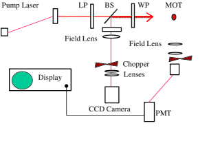
Figure 1: A schematic diagram of a typical experimental arrangement. Shown in the figure is a magneto optical trap (MOT), linear polarizers (LP) which select the detected polarization channels, a beam splitter (BS), wave plates (WP) and a photomultiplier tube (PMT) to detect the fluorescence signals for time dependent measurements. For continuous wave measurements, a charge-coupled device (CCD) camera is used. The generic display is a multichannel scalar for time dependent measurements.

Depending on the experiment to be performed, light scattered by the atoms is detected either in the backward direction on a liquid nitrogen cooled charge-coupled device (CCD) camera or in a direction at some other angle relative to the incident probe beam using a photomultiplier tube (PMT).

III.2 Coherent Backscattering Measurements

For measurements of the CBS cone, great care must be taken to suppress multiple and back reflections from optics in the detection optical path. A major source of unwanted back-scattered light is from the vacuum viewports on the MOT chamber. Windows are typically wedged and V-type anti-reflection (AR) coated for 780 nm on the probe laser entrance and exit ports and on the CCD camera. The AR coating characteristically results in less than 0.25 % reflectivity at 780 nm. Additionally, the entrance port window can be mounted on a ultrahigh vacuum bellows, allowing redirection of unwanted reflections away from the detector.

After exiting the fiber, the probe beam was expanded and collimated by a beam expander to a 1/e² diameter of about 8 mm. The polarization of the resulting beam was selected and then the beam passed through a nonpolarizing and wedged beam splitter that transmits approximately half of the laser power to the atomic sample. The backscattered radiation is directed by the same beam splitter to a field lens of 45 cm focal length, which condenses the light on the focal plane of the CCD camera. The diffraction limited spatial resolution was about 100 $\mu$rad, while the polarization analyzing power is greater than 2000 at 780 nm. Any one of the four polarization channels that are customarily studied in coherent backscattering can be selected by inserting or removing the quarter wave plate, and adjusting the linear polarization analyzer located before the field lens.

III.3 Time-Dependent Scattering Measurements

For measurements of time-dependent light scattering, light signals are detected in a direction away from the coherent beam. In a typical geometry, as shown in Figure 1, detection could be in a direction orthogonal to the probe laser propagation and polarization directions. For example, in Ref. Balik , the light was collected in an effective solid angle of about 0.35 mrad, and refocussed to match the numerical aperture of a 400 $\mu$m multimode fiber. A linear polarization analyzer is placed between the MOT and the field lens to collect signals in orthogonal linear polarization channels, which we label as parallel ($\|$) and perpendicular ($\bot$). The differential polarization response is calibrated against the known linear polarization direction of the probe laser, and the measured 20 % difference in polarization sensitivity is used to correct the signals taken in the two polarization channels. The fiber output is coupled through a 780 nm (5 nm spectral width) interference filter to a near-infrared sensitive GaAs-cathode photomultiplier tube. The PMT output is amplified and directed to a discriminator and multichannel scalar, which serves to time sort and accumulate the data into 5 ns bins. A precision pulse generator is used to control the timing of the MOT and probe lasers and for triggering the multichannel scalar.

Finally, we point out that in this type of experiment the quantitative results obtained depend on the relative diameter of the pumping beam and the sample size. The main effect is in the contribution of single scattering in comparison with the multiple scattering signals. For a pump beam large in comparison with the samples, there is significant single scattering from the relatively low density periphery, while for a narrow probe beam a larger portion of the signal is due to scattering from the denser regions of the sample.

IV CBS observation in an ultracold atomic gas in the continuous wave regime

IV.1 The enhancement factor and cone shape

First observation of the CBS effect in an ultracold atomic gas was reported by Labeyrie et al. in Ref. LTBMMK . In Figure 2 we reproduce the experimental graph from that paper showing the cone feature in the spatial profile of the backscattered light. The experiment was done with atoms of ⁸⁵Rb and the scattered light was observed as a response to a probe laser tuned near-resonance with the closed hyperfine transition $F_{0}=3\to F=4$ of the rubidium $D_{2}$ line. The rubidium atoms form a convenient sample for measurements and the dependence of Figure 2 shows a typical behavior of the CBS cone from an ensemble of these atoms. The measurements shown in Figure 2 LTBMMK were made with a circular polarized cw monochromatic probe laser, and the scattered light was detected in the channel with orthogonal helicity, which relates to the Rayleigh process for the single scattering event.

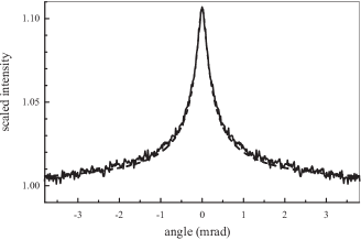
Figure 2: A coherent backscattering cone in the helicity non-preserving channel associated with the $F_{0}=3\rightarrow F=4$ transition in ultracold atomic ⁸⁵Rb. Reprint of Fig. 3 from Ref. LTBMMK ; copyright 1999 by the American Physical Society.

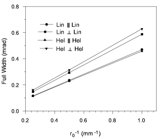
Figure 3: Dependence on the inverse sample size of the full width at half maximum of the coherent backscattering cone for various polarization channels. The peak optical depth is fixed at five for these calculations. Calculations refer to Monte-Carlo simulations of light scattering on the $F_{0}=3\rightarrow F=4$ resonance transition in ultracold atomic ⁸⁵Rb.

The graph shown in Figure 2 gives us the following two important parameters of the CBS process. The main informative parameter is the so-called enhancement factor, which is defined as

$$\alpha=1+\frac{I_{C}}{I_{L}+I_{S}}$$ (1)

and shows the maximum enhancement of the backscattered intensity. As was discussed in the theoretical overview, the additional intensity in the scattered light is a result of constructive interference between direct and reciprocal scattering paths and is described by the cross terms $I_{C}$ in the numerator of (1). The denominator consists of the single scattering contribution $I_{S}$ and non-interfering ladder contributions $I_{L}$ of the second and higher orders of multiple scattering. As is clear from the structure of Eq. (1), for classical type dipole scatterers with only Rayleigh scattering channels, the enhancement factor $\alpha$ should approach $2$ if the optical depth $b_{0}$ tends to infinity. But it is also clearly seen that this is not the case for the experimental graph shown in Figure 2.

As was pointed out later in JMKMD the relatively small magnitude of the enhancement factor is a direct consequence of multi-Zeeman-level atomic structure. The physics of the process was reiterated within an analytical microscopic theory developed by Müller, et al. Muller . The enhancement of a factor of two can be achieved only if direct and reciprocal scattering amplitudes describe the time reversal processes. Otherwise, for weak field scattering, the interference always leads to an enhancement less than a factor of two. Recovery of the factor of two in the enhancement factor was clearly demonstrated in experiments on atomic Sr by Bidel, et al. Strontium1 ; in this case scattering is on a $J_{0}=0\rightarrow J=1$ transition. The differences between the Sr and Rb cases, including the role of nonzero atom velocity, was emphasized in Wilkowski, et al. Wilkowski1 . Finally, we point out that the interferences in coherent backscattering can be destructive in special scattering channels. Below we discuss such an example of destructively interfering channels, where the enhancement factor is less than unity.

The second important characteristic of the cone shape is its angular width. For simple evaluation and as a pedagogical model, one can imagine a semi-infinite homogeneous medium and apply the diffusion approach to estimate the statistical distribution of spatial separations of the first and last scatterers in a scattering chain. It is only the location of these scatterers that determines the phase of the interference in the cross term. This straightforwardly leads to the following estimation of the cone angle

$$\theta_{\rm CBS}^{\prime}\sim\frac{1}{kl_{0}}$$ (2)

where $l_{0}=1/n_{0}\sigma_{0}$ is the free path for a resonance photon migrating in the sample, $n_{0}$ is the density of scatterers and $\sigma_{0}$ is the resonance cross section. However the application of this estimation to real experiments with atomic scatterers confined in a MOT fails and quantitatively disagrees with observable data.

As was shown by precise Monte-Carlo modelling in KSKSH , and was also discussed in LDMMK , the cone angular width does not depend on the diffusion length in the case of an atomic cloud with a Gaussian-type density distribution. For the density distribution

$$n(r)=n_{0}\,\exp(-\frac{r^{2}}{2r_{0}^{2}})$$ (3)

where $n_{0}$ is a peak density in the middle of the cloud and $r_{0}$ is the radius of the cloud, the relevant estimation of cone angle is given by

$$\theta_{\rm CBS}\sim\frac{1}{kr_{0}}$$ (4)

This is illustrated by the respective dependencies shown in Figure 3, which shows the linear dependence of the cone width on inverse sample size $r_{0}^{-1}$ in various polarization channels of the $F_{0}=3\to F=4$ transition of ⁸⁵Rb. Since for the Gaussian cloud the optical depth is given by $b_{0}=\sqrt{2\pi}\sigma_{0}n_{0}r_{0}$ we see that the estimations (2) and (4) differ by a factor of $b_{0}$ and expression (2) gives a larger cone angle width than is actually measured.

The CBS images in the plane orthogonal to the incident and backscattered directions are different for different polarization channels. Normally the polarization channels are discussed for circular and linear input and output polarizations. Circular polarization is normally defined in terms of helicities (hel) with respect to the frame of wave propagation, while linear polarization directions (lin) are defined with respect to a laboratory frame. The scattered light is detected either in the same polarization channel as the input light or in an orthogonal polarization channel. There is a spatial asymmetry in the linear polarization channel. This includes a larger cone width in the vertical direction for the lin $\parallel$ lin channel with the lines of asymmetry along the bisectors of the detected linear polarization directions in the lin $\perp$ lin channel. The details of the features in the cone shape are discussed in Ref. KSBHKS .

IV.2 The influence of hyperfine structure

In initial studies of coherent backscattering in atomic samples, it was assumed that for near-resonance scattering the hyperfine structure of the excited atomic state is unimportant (other than for the degeneracies of the transitions under consideration). Particularly for the $F_{0}=3\to F=4$ ”closed” transition in ⁸⁵Rb the nearest hyperfine satellite $F_{0}=3\to F=3$ is located at $-120$ MHz, see Figure 4. This is about $20$ times the natural line width $\gamma\sim 5.9$ MHz and argues for the unimportance of the off-resonant transitions. However as was predicted in KSKSH there is an asymmetry in the CBS enhancement for the spectral scanning near the resonance, this being caused by the interference among all the hyperfine transitions. The asymmetric shape is more clearly seen in the case of circular polarization. This indicates the non-trivial spectral behavior of the Raman-type cross/interference terms and the Raman-type ladder terms near the resonance.

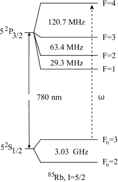
Figure 4: Hyperfine energy levels of relevant transitions in atomic ⁸⁵Rb.

The experimental verification of this effect was made in KSLKSBH ; LDMMK1 and in Figure 5 we reproduce the illustrative graph from KSLKSBH for the helicity preserving scattering channel. In the calculations the influence of possible heating effects, where the Doppler broadening $kv_{0}$ ($v_{0}=\sqrt{2k_{B}T/m}$ is the most probable velocity in the atomic ensemble) was varied from $0$ to $0.25\gamma$. The heating mechanism makes the enhancement weaker but the spectral shape broader. Comparing the results one can see that there is a qualitative agreement between theoretical calculations and experimental data. However they differ quantitatively and the enhancement, observed in the experiment in the wings, is even larger than its theoretical prediction. As was mentioned in KSLKSBH the main possible reason of such a contradiction between experiment and theory is in the optical pumping process, which tends to orient atomic spins along the probe beam. For 100% orientation this effect can increase the enhancement up to maximum value of two. The enhancement of a factor of two would be achievable because for spin oriented ensemble there is no the single scattering contribution. Then there would be only two constructively interfering amplitudes if the double scattering channel could be isolated. This effects is similar to the enhancement factor behavior in a strong magnetic field, as discussed in the following section.

We conclude this section by emphasizing that there are also significant variations in the enhancement factor even for resonant scattering on different $F_{0}\rightarrow F$ transitions. This is due primarily to the different degeneracies associated with the transitions. Experimental confirmation of these variations, and comparisons with Monte-Carlo and model calculations have recently been reported by Wilkowski, et al. FrenchHyperfine .

IV.3 Influence of an external magnetic field

The influence of an external magnetic field on the multiple scattering in optically dense atomic ensembles was studied in Refs. LMK ; LMMSDK ; SLJDKM . The unique conditions of ultracold atomic ensembles, where there is negligible inhomogeneous Doppler broadening, make possible the spectroscopic manipulation with a magnetic field for the Zeeman splitting of the atomic levels at the level of the natural line width. In Ref. LMK , which has no direct relation to the CBS phenomenon, the Faraday rotation of quasi-resonant light in an optically thick cloud of laser cooled rubidium atoms was experimentally studied. Measurements yield a large Verdet constant in the range $200000^{0}$/T/mm and a maximal polarization rotation of $150^{0}$. The Faraday effect was initiated

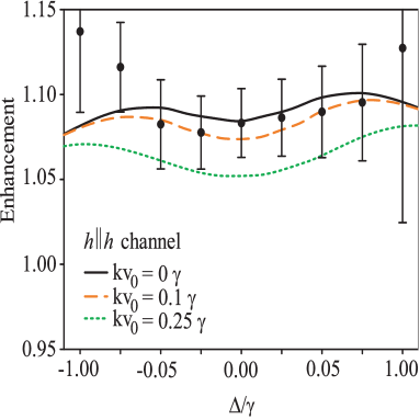
Figure 5: Comparison of experimental and theoretical enhancement spectra in the helicity-preserving polarization channel associated with an $F_{0}=3\rightarrow F=4$ resonance transition. Theoretical spectra show modification by Doppler broadening, which is varied from $kv_{0}=0$ to $kv_{0}=0.25\gamma$, in an ensemble of ⁸⁵Rb atoms having a peak density of $n_{0}=1.6\times 10^{10}$ cm^-3 and a Gaussian radius $r_{0}=1$ mm.

by the Zeeman splitting in the ground and in the upper state, which led to differences in the refraction indices for $\sigma_{+}$ and $\sigma_{-}$ polarization of the probe light. It is just the absence of the Doppler effect and the possibility to scan the sample near the natural resonance line which permits such a huge Verdet constant to be obtained.

As a next step it was recognized that a weak magnetic field, with Zeeman splitting comparable with the natural line width, should modify the CBS process itself. The presence of the magnetic field manifests itself in the scatterer dipole response to the electric field in a manner similar to the Hanle effect in a fluorescence geometry. As was shown in experiment LMMSDK the polar shape of the CBS cone in the linear polarization scattering channel follows the magnitude and direction of the magnetic field vector. In the theoretical discussion of Ref. LMMSDK an attempt was made to classify the influence of a magnetic field in terms of the well known Faraday, Cotton-Mouton and Hanle effects. But as is clear in multiple scattering, and particularly in the multiple scattering regime of CBS, there is only a convenient analogy with these basic optical processes.

The remarkable manifestation of a magnetic field was recently observed in Ref. SLJDKM . There it was observed that the enhancement factor can be increased with magnetic field up to its maximal value of two. This unusual behavior appears due to lifting of degeneracy in the helicity scattering channel for the spectrally selected Zeeman hyperfine transition $F_{0}=3,M_{0}=3\to F=4,M=4$ of ⁸⁵Rb, which can be done by applying a rather strong external magnetic field. For this transition there is no Raman-type scattering in the single scattering response. If only double scattering dominates in the helicity preserving scattering response there should be a factor of two enhancement of the scattered intensity. In the Figure 6 we reproduced the basic graph of SLJDKM , showing the experimental verification of this effect. Let us also point out that there is a direct analogy of the behavior of the enhancement factor in a magnetic field with its spectral behavior in a spin-oriented ensemble predicted in KSLKSBH .

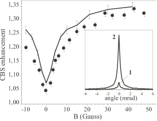
Figure 6: CBS enhancement factor of light for a cold Rb atomic cloud, measured in the parallel helicity channel hel $\parallel$ hel, as a function of the transverse magnetic field strength $B$; the graph shows an increase in the CBS enhancement for non-zero magnetic field. The solid line is the result of a Monte-Carlo simulation. The inset shows profiles of the CBS cones when $B=0$ (1) and $B=43$ G (2). Reprint of Fig. 2 from Ref. SLJDKM ; copyright 2004 by the American Physical Society.

IV.4 The CBS process in the saturation regime

Recent experiments by Chaneliere, et al. Chaneliere on the resonance transition in atomic strontium and by Balik, et al. Balik in rubidium, have shown that a significant reduction in the coherent backscattering enhancement can occur with increasing intensity of the probe laser. Both non-linear effects and additional inelastic scattering components can contribute to this reduction. Theoretical and model studies have shown similar qualitative effects Wellens1 ; Shatokhin ; Wellens2 , although they have yet to be quantitatively compared with experiment.

In the strontium experiment, a MOT containing 7$\times$10⁷ atoms at a temperature of $\sim$1mK and with a Gaussian radius of $\sim$0.7 mm was illuminated with near resonant light. The ensemble of cold atoms had a peak optical depth of $b_{0}$ = 3.5 and $\emph{kl}_{0}=10^{4}$, resulting in a regime of weak localization. In the absence of MOT light and magnetic field gradients, a resonant probe beam illuminated the sample for a variable period of 5 to 70 $\mu$s. The probe pulse duration was adjusted so as to keep the total number of scattered photons below 400 for all intensities investigated, thereby minimizing mechanical effects of the light on the cold atom sample. A CBS cone was then recorded in the helicity preserving channel (hel $\|$ hel), where single scattering is negligible. Keeping the shape of the CBS beam constant, but treating the width and enhancement factors as free parameters, a CBS cone enhancement was extracted. Results for on resonance scattering and a detuning of $\delta=\Gamma/2$ were measured as a function of saturation parameter $s=I/I_{s}$, where $I_{s}$=42 mW/cm². The results indicate that saturation is in part responsible for the magnitude of the cone enhancement, but saturation alone does not fully describe the CBS process. Detuning also plays a role because the ratio of inelastic to elastic scattering is detuning dependent. It is the inelastic component which degrades reciprocity and causes the enhancement factor to decrease. As the field increases, the inelastic nature of the light scattered also increases yielding a decreasing cone enhancement factor.

In the rubidium experiment, a nearly spherical MOT containing $\sim 4\times 10^{8}$ at a peak density of $1.6\times 10^{8}$ atoms-cm^-3 was illuminated with a probe beam for time T and the CBS cone was recorded on a liquid nitrogen cooled CCD camera as described in Section 3. Two polarization channels, lin $\bot$ lin and hel $\|$ hel were investigated. The intensity of the backscattered light was detected and the enhancement factor of the CBS cone measured as a function of probe intensity, again expressed in terms of the saturation parameter s, where $I_{s}$ in this case is the on-resonance saturation intensity of about 1.6 mW/cm². Data taken at s=0.08 provided the baseline for the “weak” field cone measurements. The baseline saturation parameter and exposure time were selected to minimize mechanical action of the CBS laser on the cold atom sample as in the Sr experiment. With s = 0.08, a probe exposure time of T = 0.25 ms satisfied this condition.

Measurements up to a saturation parameter of 9 in the lin $\bot$ lin channel were made. For optical depths larger than unity (as is the case here), one expects the width of the cone to be determined primarily by the spatial distribution of atoms in the MOT and not be very sensitive to the saturation parameter. Indeed, little change in the angular width of the cone was observed, in agreement with theory and the experimental results of Ref. Chaneliere . The cone enhancement factor $\alpha$, however, was observed to decrease substantially in the strong field regime. Cone images for the lin $\bot$ lin channel are shown in Figure 7. In this data, the product sT was constant and the total spatially integrated intensity was the same in all four images.

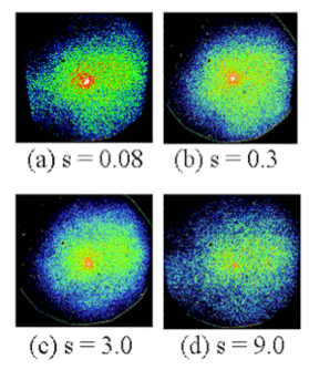
Figure 7: Dependence on the saturation parameter s in the lin $\bot$ lin polarization channel, of CCD images of the intensity field in the nearly backscattering direction. The data correspond to the $F_{0}=3\to F=4$ hyperfine resonance in ⁸⁵Rb.

The data, which spans a saturation parameter range of more than 100, shows a clear reduction in the contrast of the cone with increasing intensity. This behavior is shown quantitatively in Figure 8, where it is seen that the enhancement $\alpha$ decreases with increasing saturation parameter over the data range explored. As previously discussed, a similar monotonic decrease in $\alpha$ has been observed in experiments on the singlet resonance transition in ultracold Sr Chaneliere . However, the percentage decrease in $\alpha$ with increasing s was observed to be much larger in that case than in the Rb experiments.

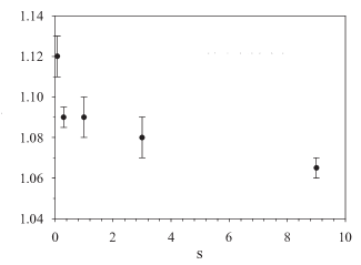
Figure 8: Dependence of the coherent backscattering enhancement on the saturation parameter s in the lin $\bot$ lin polarization channel. The data correspond to the $F_{0}=3\to F=4$ hyperfine resonance in ⁸⁵Rb.

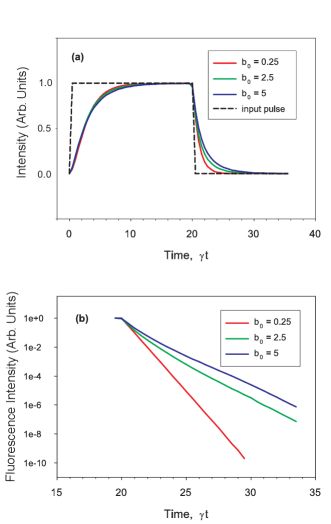
Figure 9: (a) The intensity response for light scattered in the backward direction from an atomic sample of ⁸⁵Rb probed by a pulse with a duration of $\tau_{0}=20\,\gamma^{-1}$ tuned to resonance with the $F_{0}=3\to F=4$ hyperfine transition for different optical thicknesses $b_{0}$. (b) Fluorescence decay after the excitation pulse is switched off.

Measurements of $\alpha$ in the hel $\|$ hel channel (not shown) in the range 0.04 $\leq$ s $\leq$ 1.0 stay relatively constant - in sharp contrast to the results for the lin $\bot$ lin channel and to the results of Chaneliere, et al. Chaneliere . The approximate constancy of $\alpha$ is a surprising result and suggests that optical pumping of the Zeeman sublevels in the ground level may play an important role in the observed quantitative results. Several other possible physical mechanisms explaining the data have been suggested in Balik but await confirmation by detailed calculations.

V Time-dependent and spectral analysis of the scattered light

V.1 Time dependent spectroscopy in a backscattering geometry

Consider excitation of an atomic ensemble with a coherent light pulse, when the correlation function can be factorized in the form (8). Let the field amplitude of ${\cal E}_{\mu}^{(+)}(\mathbf{r},t)$ have a rectangular pulse profile. It is convenient to scale the duration of the pulse $\tau_{0}$ by the natural atomic lifetime $\gamma^{-1}$. In accordance with (II.1) and with the usual restrictions of the rotating wave approximation, the rectangular pulse profile should be expanded over the set of incoming modes with the following amplitude

$$\alpha_{\mathbf{k}\mu}\propto\frac{\exp[i(\omega_{k}-\omega)\tau_{0}]\,-\,1}{i(\omega_{k}-\omega)\tau_{0}-0}\;e_{\mu}$$ (1)

describing the pulse propagating along the $z$-axis with carrier frequency $\omega$, mode wave vector ${\mathbf{k}}\parallel z$, mode frequency $\omega_{k}=c\,k$ and polarization ${\mathbf{e}}$. The pulse wavefront arrives at the plane $z=0$ at the time $t=0$ and $\alpha_{\mathbf{k}\mu}$ are the eigenstates of the mode annihilation operator:

$$a_{\mathbf{k}\mu}|\alpha_{\mathbf{k}\mu}\rangle=\alpha_{\mathbf{k}\mu}\,|\alpha_{\mathbf{k}\mu}\rangle$$ (2)

This initial coherent state gives an expected number of photons arriving at the system during the interval $(0,\tau_{0})$.

For an isotropic Gaussian-type cloud, with a radius normally on the order of $1$ mm, the Green’s Function (7) can be expressed in the form (6), where for an isotropic medium the slowly varying amplitude is given by

$$X_{ij}(\mathbf{r}_{1},\mathbf{r}_{2},\omega)=\delta_{ij}^{\perp}\,\exp\left[-\frac{2\pi\omega}{c}\int_{{\mathbf{r}}_{1}}^{{\mathbf{r}}_{2}}\,\chi({\mathbf{r}},\omega)\,ds\right]$$ (3)

where the integral is evaluated along the ray $s$ linking the points ${\mathbf{r}}_{1}$ and ${\mathbf{r}}_{2}$, and $\chi({\mathbf{r}},\omega)$ is the local susceptibility of the inhomogeneous medium, see definitions (13), (14).

In Figure 9(a) we show how the originally rectangular pulse (1) with duration of $\tau_{0}=20\,\gamma^{-1}$ is distorted in the scattering response in the backward direction. The calculations were made for the resonance $F_{0}=3\to F=4$ hyperfine transition of the $D_{2}$ line of ⁸⁵Rb for the optical thicknesses $b_{0}$ varying in the interval from $0$ to $5$. During such a long probe of the sample the steady state behavior, established within the temporal duration of the pulse, is clearly indicated. But the sharp shapes of initial and final fronts of the pulse are smoothed in the response pulse because of the delay in multiple scattering of different orders. The dependence on optical thickness emphasizes that this delay is longer as the scattering in higher orders becomes more important, i. e. for higher $b_{0}$. In turn, as shown in Figure 9(b), the presence of different scattering orders in the outgoing response also manifests themselves in multi-exponential decay of the fluorescence, which approximately approaches the zero Holstein mode for a rather long time and for high $b_{0}$.

The importance of the response inertia is remarkably indicated in the time dynamics of the enhancement factor for the CBS process. For a time dependent process the enhancement factor should be defined by the ratio of the instantaneous intensity of light scattered in the backward direction at the moment $t$ to the contribution of the single scattering and only ladder-type terms of the higher orders of multiple scattering

$$\alpha(t)=1+\frac{I_{C}(t)}{I_{S}(t)+I_{L}(t)}$$ (4)

Here $I_{S}(t)$, $I_{L}(t)$, $I_{C}(t)$ are respectively the single, ladder and crossed (interference) contributions to the instantaneous outgoing intensity.

In Figure 10 we illustrate the time dependence of the enhancement factor calculated in the same conditions and for the same parameters as the intensity response in Figure 9. The most interesting is a break point on the graph corresponding to the moment when the probe pulse is switched off. During the decay process the enhancement factor rises up at the beginning stage and drops down only after a delay and with a slower rate. Such behavior is a direct consequence of the intensity decay shown in Figure 9. Since the single scattering disappears first then, in accordance with definition (4), it should be expected that the instantaneous value of the enhancement factor will be raised immediately after the pulse is switched off.

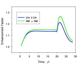
Figure 10: Time-dependence of the enhancement factor for the excitation conditions of Figure 9 in the lin $\|$ lin parallel and hel $\bot$ hel scattering channels. The optical thickness $b_{0}$ is equal to $5$ for this graph.

As one can see, the time dependent analysis gives us certain spectroscopic access to the selective information about different orders of multiple scattering. The CBS phenomenon could be an important process for this. If the sensitivity of time dependent measurements were high enough then the long-term decay of the instantaneous value of the enhancement factor would strongly select the contribution of different scattering orders. Roughly we would say that the time decay shown in Figure 10 just copies the partial contribution to the enhancement coming from different orders of multiple scattering. To show this in Figure 11 we plot the calculated data for the partial contributions to the enhancement factor for the scattering orders from two up to five. As one can see there is a qualitative coincidence between the graphs showing the time decay and the dependence on scattering order. Both the dependencies approach the value of unity because in higher scattering orders the number of non-interfering amplitudes enlarges faster than the number of interfering ones.

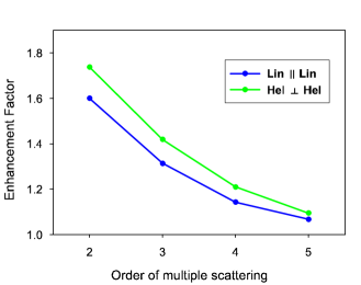
Figure 11: Partial contributions to the enhancement factor as function of the order of multiple scattering for the same polarization channels as in Figure 10.

In discussions of the CBS process in the literature Sheng ; LagTig the cone profile itself is normally suggested as an experimental reference dependence for selecting different orders of multiple scattering. Such a spatial spectroscopy method utilizes an idea that the higher orders contribute and are localized near the peak point of the cusp-like CBS cone. As is clear from the above discussion, in the time dependent spectroscopy there is an alternative situation when higher orders contribute in the wing of the time decay of the enhancement factor. Thus the spatial spectroscopy and time dependent spectroscopy could be complementary techniques for study of the weak localization of light in disordered media.

V.2 Measurements of time dependent diffuse light intensity

To date, there have been no measurements of the time dependence, in ultracold atomic gas samples, of coherently backscattered light. However, there have been several experimental studies, in ultracold gas samples, of the time dependence of multiply scattered light Balik1 ; Fioretti ; LabeyrieTime1 . In this section we present some of our combined experimental and theoretical results on the polarization dependence of multiple light scattering in ultracold atomic ⁸⁵Rb.

The essential experimental details Balik1 are discussed in Section 3 of this report. In these experiments, the intensity of light emitted in a direction orthogonal to the excitation light source is measured as a function of time and linear polarization state. These dependences are illustrated in Figure 12, which shows the measured intensities in two orthogonal polarization channels for resonance excitation of the $F_{0}=3\rightarrow F=4$ hyperfine transition. In the figure, the scale of the peak intensity in the lin $\|$ lin channel is about 10⁴ counts. In this data, the transient build up is due to multiple scattering of probe radiation after it has been switched on. The time scale for the process can be seen more clearly in the expanded view in the lower panel of Fig. 12. The solid curves in Fig. 12 represent Monte-Carlo simulations of the scattering process. Other than the overall intensity scale, there are no adjustable parameters in the comparison, with the simulation input data consisting of the measured trap density profile and peak optical depth.

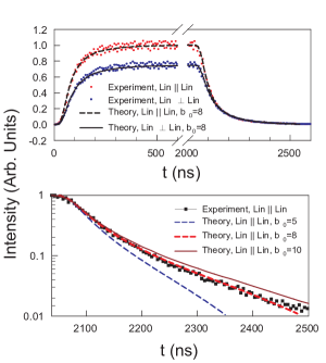
Figure 12: Measured time-dependent scattered light signal in orthogonal linear polarization channels. Theoretical results are indicated by the curves, as labelled in the figure legend.

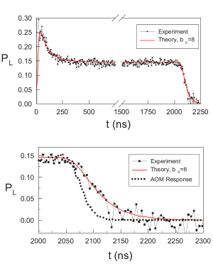
Figure 13: Measured time-dependent linear polarization degree, shown as solid points. Monte Carlo simulation results are shown as solid lines, while the limiting AOM response is shown as a dotted line.

This data is further reduced to emphasize the intensity differences for the two orthogonal linear polarizations. This is done by defining a linear polarization degree as

$$P_{L}=\frac{I_{\parallel}-I_{\perp}}{I_{\parallel}+I_{\perp}}$$ (5)

In the formula, $I_{\parallel}$ and $I_{\perp}$ represent the measured intensities in the lin $\parallel$ lin and lin $\perp$ lin channels. The data in Fig. 12 then give the time-dependence of $P_{L}$ shown in Fig. 13. There we see that $P_{L}$ enhances the differences in the different channels, thus clearly showing the time-dependent maximum in $P_{L}$ soon after the exciting pulse is turned on, which is followed by approach to a steady state linear polarization degree. We point out that the peak value of $P_{L}$ corresponds to a predominately single scattering value of $P_{L}$ = 0.268 for this resonance transition. As seen in the lower panel of Fig. 13, once the probe laser is turned off, $P_{L}$ rapidly decays toward 0. This emphasizes the quite different time scales for decay of the population in comparison to that of the electronic alignment. In all of this data, the Monte-Carlo simulations do an excellent job of describing both the light intensity and polarization dynamics in the system.

Finally, it is important to note that the spectral dependence of diffuse light scattering is strongly influenced by interferences in the light scattering amplitudes from different excited hyperfine levels. This is illustrated in Figure 14, which shows the spectral variation of the steady state linear polarization degree. In the figure, if hyperfine interferences were absent, the single scattering atomic polarization would be very nearly constant over the spectral range of the figure. We should point out that there is a much more gradual variation of the linear polarization due to coherent excitation of the fine structure multiplet levels.

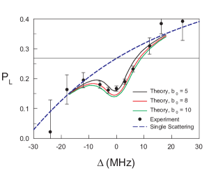
Figure 14: Detuning dependence of the linear polarization degree. The horizontal line indicates the single scattering benchmark at 0.268. The dots represent the experimental data points, while the blue chained curve is the expected variation for single atom scattering. The red and blue curves indicate the polarization variation for optical depths of $b_{0}=5$ (black), $b_{0}=8$ (red), and $b_{0}=10$ (green).

Instead, we see strong variations in the measured polarization due to both multiple light scattering and due to hyperfine interferences. For example, as the magnitude of the detuning is made larger, the measured steady-state values for $P_{L}$ approach the calculated frequency-dependent single scattering limit for this transition. Near the resonance, the polarization is significantly reduced by multiple coherent scattering. In all cases, agreement with Monte Carlo simulations is very satisfactory.

V.3 Spectral distribution of the scattered light

As an alternative to the time dependent analysis, it is possible to determine the spectral selection of the multiple scattering process. Different orders of the scattering should have different spectral profiles in response to coherent monochromatic excitation. In an experiment, precise selection can be done by using the light beating spectroscopy technique Lightbeating . In this approach, mixing the scattered light with a local oscillator wave in a heterodyne detection scheme yields a photocurrent spectrum which will reproduce the spectrum of the scattered light given by (9) and (10).

This spectrum can be calculated analytically if the following three basic criteria are met. (i) The velocity distribution for the atoms in the trap should be of the Maxwell-Boltzmann type. (ii) Near the Doppler cooling limit the corresponding Doppler frequency shift is much less than $\gamma$ and the retarded and advanced type Green functions should be insensitive to the atomic velocity distribution. (iii) For the same reason, the dependence of the scattering amplitude on atomic velocity should be also negligible for deeply cooled atoms. Then for the $N$-th order of multiple scattering the partial spectral profile will be centered at the either the Rayleigh elastic or Raman shifted outgoing frequency $\omega_{R}$ and will be given by

$$I_{N}(\omega)=\left\langle I_{N}\,\sqrt{\frac{2\pi}{\Gamma_{N}}}\,\exp\left[-\frac{(\omega-\omega_{R})^{2}}{2\Gamma_{N}^{2}}\right]\right\rangle$$ (6)

where the Gaussian bandwidth is given by the following sum

$$\Gamma_{N}=\frac{1}{\sqrt{2}}\left[\sum_{i=1}^{N}|\Delta{\mathbf{k}}_{i}|^{2}\right]^{1/2}{v_{0}}$$ (7)

Here $\Delta{\mathbf{k}}_{i}$ with $i=1\div N$ is the sequence of changes of the wave vector for the scattering of the light wave along any randomly selected scattering chain consisting of $N$ atoms. Here the velocity $v_{0}$ is the most probable velocity for the respective Maxwell-Boltzmann distribution, see definition in section IV.2. $I_{N}=I_{N}({\mathbf{r}}_{1},\ldots{\mathbf{r}}_{N})$ is the total intensity of the fraction of the light scattering in the direction of observation by the subsequent scattering from atoms located at spatial points ${\mathbf{r}}_{1},\ldots{\mathbf{r}}_{N}$. The angle brackets in (6) denote the averaging over the spatial distribution of these atoms. Such an averaging extends over $\Delta{\mathbf{k}}_{i}$ and $\Gamma_{N}$ as well, which also depend on the locations of atoms, see definitions (2), (3). Then the total spectrum of the scattered light is given by

$$I(\omega)=\sum_{N}I_{N}(\omega)$$ (8)

It is remarkable that this result is valid for the scattering in any direction including backscattering. The interference terms have the same spectral profile as the ladder terms if the atoms do not noticeably change their location on the spatial scale of $\lambda/2\pi$ during the retardation delay while the light wave passes through the scattering chain. As one can see in higher orders of multiple scattering the spectrum becomes broader and for an isotropic sample the bandwidth $\Gamma_{N}$ is enhanced by $N$.

However in reality the assumptions (i) - (iii) are not exactly fulfilled. First, the velocity distribution is only approximately Maxwell-Boltzmann-type because of complexity of the cooling mechanism in MOT. Second, if the Doppler scale $kv_{0}$ is comparable with the natural line width $\gamma$, there will be additional damping mechanisms acting via the Green’s propagator phase, reducing the scattering amplitude. Thus the sum of Gaussian profiles (8) gives us only a convenient zero-level approximation, or a certain type of reference dependence for further spectroscopic analysis. The deviations from this basic dependence provide us with actual information about real atomic motion and spatial correlations of atoms in the sample.

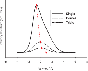
Figure 15: Spectral profiles of the light backscattered on the $F_{0}=3\to F=4$ hyperfine transition of ⁸⁵Rb in Rayleigh-type lin $\parallel$ lin polarization channel for different orders of multiple scattering. The probe light frequency is shifted to the blue wing of the resonance by one natural line width $\gamma$ and the velocity distribution of atoms is assumed to be Maxwell-Boltzmann-type with $kv_{0}=\gamma$. The red circle indicate how the maxima approach the limit of elastic scattering $\omega_{R}=\omega_{43}+\gamma$ in higher orders.

We illustrate this in Figure 15 where we show typical dependencies of the spectral response on the monochromatic probe wave for the scattering near the backward direction in the lin $\parallel$ lin polarization channel from atoms of ⁸⁵Rb. The data are presented for the $F_{0}=3\to F=4$ hyperfine transition of the $D_{2}$-line and for the different orders of multiple scattering. The frequency of the probe wave is tuned to the blue wing from the atomic resonance by one natural line width $\omega_{43}+\gamma$. The velocity distribution is assumed to be Maxwellian with $kv_{0}=\gamma$. For such ”hot” atoms the ladder-type response is mainly important in the detection channel. For Rayleigh-type scattering initiated on the selected closed transition the carrier frequency is $\omega_{R}=\omega_{43}+\gamma$ and, according to (6), it is expected that the spectral response should be centered and distributed near this carrier frequency shifted to the blue wing of resonance. But as one can see this is not the case and the mean frequency of the scattered light is shifted to the red wing of the atomic resonance. This is a typical manifestation of the Doppler effect in the denominators of scattering amplitudes. In a single scattering event, the scattering is preferably organized from the atoms moving with $v_{z}\sim\gamma/k$ in the direction of the incoming wave front. Thus the outgoing wave, which is scattered from these atoms, will be shifted by $-2kv_{z}\sim-2\gamma$. In a weaker form such an effect is preserved for the double and triple scattering channels, as also shown by the corresponding dependencies of Figure 15.

In Figure 16 we show how the spectral profiles for the total ladder and interference contributions depend on the frequency of the probe light, which is varying from the resonance transition frequency $\omega_{43}$ up to $\omega_{43}+2\gamma$. Other parameters are the same as in Figure 15. As is clearly seen, the location of the maximum for the ladder portion shifts to the red wing for small detuning and approaches the frequency of elastic scattering $\omega_{R}$ only for large detunings. For interference terms, the location of the maximum shifts approximately as $\omega_{R}$, which is because of no single order contribution in this case.

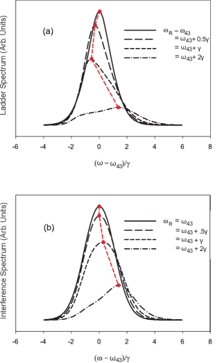
Figure 16: Spectra of the ladder (a) and interference (b) contributions to the light backscattered on the $F_{0}=3\to F=4$ hyperfine transition of ⁸⁵Rb for different frequency offsets of the probe light from the resonance transition. Other parameters are the same as in Figure 15. The red circles trace the location of the maxima as they approach the elastic carrier frequency for far off-resonant scattering.

If atoms are cooled close to the Doppler limit, such that $kv_{0}\ll\gamma$, the spectral profile will be given by expressions (6)-(8). In this case its spectral bandwidth can be quite narrow and in an experiment a high quality monochromatic local oscillator wave should be applied to resolve the spectrum by heterodyne detection. But the possible experimental realization could give us certain access to observation of the actual velocity distribution of the ultracold atoms in the trap, which is not necessarily Maxwellian.

V.4 Polarization-sensitive effects: Anti-enhancement in weak localization regime

Let us consider an atomic ensemble consisting of atoms oriented in their angular momenta. Further, let this ensemble be probed with circular polarized light in a direction antiparallel to the magnetization direction of the atomic vapor. Such a geometry requires special preparation since, because of the optical pumping process, there is a tendency to reorient the collective spin vector of the atomic ensemble along the beam, especially following a long interaction with the probe light, and after an accumulation of a sufficient number of Raman transitions. However during the short pulsed excitation we can neglect the optical pumping mechanism and assume that most of the atoms populate the $|F_{0},m=-F_{0}\rangle$ Zeeman state. In addition, and for the reason explained below, we can assume that the ensemble is located in an external weak magnetic field directed along the light beam. Thus the photons scattered via Raman channels will be generally Raman shifted. This splitting can be made quite small and less than the natural line width of the respective optical transition but still resolved with high resolution spectroscopy techniques.

In Figure 17 we show the double backscattering of incident light of positive helicity on a system consisting of two ⁸⁵Rb atoms; the exit channel consists of detection of light also of positive helicity. The two interfering channels, which are shown here, repopulate atoms via Raman transitions from the $F_{0},m=-F_{0}$ to the $F_{0},m=-F_{0}+2$ Zeeman sublevel. In the direct path the scattering consists of a sequence of Rayleigh-type scattering in the first step and of Raman-type scattering in the second. In the reciprocal path, Raman-type scattering occurs first, and the positive helicity photon undergoes Rayleigh-type scattering in the second step. Since identical helicities in incoming and outgoing channels have opposite polarizations with respect to the laboratory frame, there is an important difference in transition amplitudes associated with the Rayleigh process for these two interfering channels. Indeed, in the direct path the $\sigma_{+}$ mode is coupled with $F_{0}=3\to F=4$, $F_{0}=3\to F=3$ and $F_{0}=3\to F=2$ hyperfine transitions. But in the reciprocal path, the $\sigma_{-}$ mode can be coupled only with the $F_{0}=3\to F=4$. As we see from the diagrams shown in Figure 17, where the probe light frequency is scanned, for example, between the $F_{0}=3\to F=4$ and $F_{0}=3\to F=3$ transitions, a unique spectral feature is found when the scattering amplitudes connecting the direct and reciprocal scattering channels are equal in absolute value but have phases shifted by an angle close to $\pi$. From an electrodynamic point of view, such conditions are realized when, due to the asymmetry in the Rayleigh-type transitions, the real part of the susceptibility of the sample is positive for the $\sigma_{-}$ mode and is negative for the $\sigma_{+}$ mode. Since, in a first approximation, the amplitudes of the processes shown in Figure 17 have opposite signs they will interfere destructively with anti-enhancement of the light scattered in the backward direction in the helicity preserving channel. Such an unusual behavior in the CBS process is connected with the Raman nature of the helicity preserving scattering channel. To observe this effect, and not have it obscured by other competitive and constructively interfering channels, both special light polarization and selection of certain atomic $\Lambda$-type transition are required.

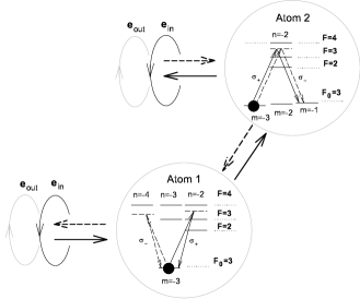
Figure 17: Diagram explaining the anti-localization phenomenon in the helicity preserving scattering channel for double scattering of circular polarized light from an ensemble of ⁸⁵Rb atoms oriented opposite to the helicity vector of the probe beam. The destructively interfering amplitudes are a combination of Rayleigh- and Raman-type transitions. The solid and dashed lines indicate the interfering direct and reciprocal scattering paths for probing between $F_{0}=3\to F=4$ and $F_{0}=3\to F=3$ hyperfine transitions.

In our example, and in the case of degenerate Zeeman sublevels, there are several competing channels of double scattering, which can interfere constructively. In an experiment, possible selection of either destructively or constructively interfering channels can be done by focusing attention to their angular dependence with respect to the location of the atomic scatterers. For an optically thin sample the process of Figure 17 dominates for atoms located preferably along the probe beam direction. The respective angular factor is proportional to the probability to initiate $\sigma_{+}$ or $\sigma_{-}$ transitions on the second atoms by the photon also emitted on the $\sigma_{+}$ or $\sigma_{-}$ by the first atom. The probability is given by

$$P_{++}(\theta)=P_{--}(\theta)\propto\frac{1}{4}(\cos^{2}\theta\,+\,1)^{2}$$ (9)

In turn, other processes are dominant if atoms are located preferably in the plane orthogonal to the probe beam. Thus in double scattering channel one can expect that, for a cigar-type atomic cloud, stretched along the probe beam direction and squeezed in orthogonal directions, the destructively interfering channels should give the dominant contribution.

In Figure 18 we show the dependence of the enhancement factor, calculated only for double scattering amplitudes, on the frequency of the probe field $\omega_{L}$. The blue curve is the contribution of the amplitudes expressed by the diagrams of Figure 17. The green curve includes the whole set of the double scattering amplitudes including all the constructively interfering channels. The calculations were made for the optical depth near the threshold level of $b_{0}\sim 1$ at each spectral detuning $\Delta=\omega_{L}-\omega_{43}$. It may seem surprising that even in this hypothetical situation, where only the process of Figure 17 contributes to the enhancement factor, it actually never drops down to zero level. This is because of the complexity of the Green propagation function in the spin polarized gas, which is discussed in an appendix. If locations of the atoms are shifted in the transverse plane, the phases of the $\sigma_{+}$ and $\sigma_{-}$ modes in the intermediate segments of the direct and reciprocal paths will be mismatched because of the refraction anisotropy of the sample. It is also unexpected that the accumulation of all the constructively interfering channels do not overwhelm the anti-localization effects in the observation conditions. The enhancement factor stays less than unity in the level of twenty percent in the total double scattering outcome. As follows from Figure 18 this takes place near the $F_{0}=3\to F=2$ resonance.

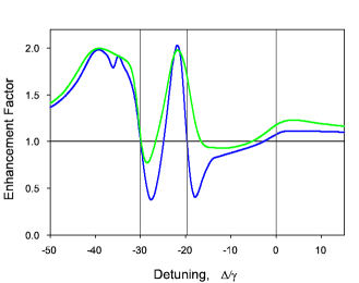
Figure 18: The enhancement factor in the helicity preserving channel for double scattering as a function of detuning $\Delta=\omega_{L}-\omega_{43}$ for the probe laser scanning the upper hyperfine manifold of ⁸⁵Rb. The blue curve shows the contribution of the processes depicted in Figure 17 and in the green curve all the constructively interfering channels were added. Vertical lines indicate the location of hyperfine resonances.

Let us briefly discuss the feasibility of how the anti-localization phenomenon could be observed in experiment. Our previous proposal KSH was based on the idea to organize an inelastic Raman type selection of the process shown in Figure 17. For this the Zeeman sublevels of the ground state could be split by external magnetic and electric fields as shown in the energy diagrams of Figure 17. Then the heterodyne detection seems a quite preferable high resolution spectroscopic technique to organize such a selection. Here we draw attention to another possibility to preferably select the double scattering, this by the time dependent spectroscopy technique described in Section V.1. As far as the decay rate of an atomic dipole is insensitive to its excitation frequency, the different orders of the multiple scattering will be subsequently observed during the time decay after the probe radiation is switched off, see Figure 10. This means that in the anti-localization regime the time dependence of the enhancement factor should be expected to break down (not up) after the probe pulse switched off. Our evaluations reproduced by the graphs of Figure 18 show that such a challenging and interesting scattering phenomenon as anti-localization of light is readily within current experimental capability.

VI Conclusion

In this review, we have provided a detailed summary of theoretical and experimental developments associated with coherent backscattering of light from ultracold samples of Rb or Sr atoms. The main observables are the coherent backscattering enhancement and the width of the backscattering cone. The paper considers the influence on these observables of a number of external parameters, including spectral variation from resonance excitation, the influence of magnetic fields, suppression of the coherent backscattering effect due to stronger electromagnetic fields. In the spectral variations, interference effects due to normally energetically distant hyperfine transitions are considered. Interference effects due to coherent scattering from nondegenerate levels are considered, including a regime of so-called antilocalization. The time evolution of the coherently backscattered light is also discussed, including the influence on the coherent backscattering cone with time. The method of light beating spectroscopy is discussed in the context of its utility in extracting additional information, including the actual velocity distribution of the atoms, regarding the light scattering process.

We emphasize that research exploring the physics of weak localization in ultracold atomic gases is clearly in the earliest stages, and there remain many unexplored lines of inquiry. Among these are fundamental aspects of nonlinear optical phenomena in the multiple scattering regime, and investigation of multifield coherences such as electromagnetically induced transparency and absorption. Research into nonlinear optics at very low light levels and the possibilities associated with generation of novel types of polaritonic excitations may have important practical applications in the area of quantum information processing. Finally, the regime of strong localization of light in ultracold gases is within reach of current experimental techniques of ultracold atomic physics. Strong light localization, as a phase transition in the quantum properties of energy transport in ultracold gases, promises fascinating opportunities for new experimental and theoretical insights into the physics of disordered systems.

Appendix A Green’s propagation function

A.1 Dyson equation

Light propagation through a sample consisting of atoms with arbitrary polarizations of their angular momenta was considered first by Cohen-Tannoudji and Laloë in Refs. ChTnLa . In those papers, such well known effects of optical anisotropy of an atomic vapor as birefringence, gyrotropy and dichroism were linked with the formalism of the irreducible tensor components of atomic polarization, i.e. with the orientation vector and alignment tensor. In the formalism of the Green’s function, the problem of light propagation through a polarized atomic vapor was discussed in Ref. KSS . The technique developed there permitted analytical solution for the Green’s function in many practically important applications. We review here the basic results of KSS and make them closer to the previously discussed conditions of CBS experiments with a cold atomic vapor confined to a MOT.

According to a general quasi-particle conception, the retarded-type Green’s function can be found as a solution of the following Dyson equation

$$\left[\frac{1}{c^{2}}\frac{\partial^{2}}{\partial\tau^{2}}-\triangle_{1}\right]D_{ij}^{(R)}(\mathbf{r}_{1},\mathbf{r}_{2},\tau)=-4\pi\hbar\delta(\tau)\delta^{\bot}_{ij}(\mathbf{r}_{1}-\mathbf{r}_{2})$$

$$+\int_{0}^{\infty}\!d\tau^{\prime}\int\!d^{3}r_{1}^{\prime}({\cal P}_{\bot}^{(R)})_{ii^{\prime}}(\mathbf{r}_{1},\mathbf{r}_{1}^{\prime},\tau^{\prime})\,D_{i^{\prime}j}^{(R)}(\mathbf{r}_{1}^{\prime},\mathbf{r}_{2},\tau-\tau^{\prime})$$

which reveals the normal vacuum wave equations modified by the contribution of the polarization operators on the right-hand side. Rigorously speaking, this equation defines only the positive frequency components of the Green’s function derived under the assumptions of the rotating wave approximation. But such an assumption is consistent with the general restrictions of our calculations and is just the Fourier image of the positive frequency components of the Green’s function, which has to be substituted into Eq.(7).

An important characteristic of equation (LABEL:A.1) is the transverse delta-function, which is given by

$$\delta^{\bot}_{ij}({\mathbf{r}})=\delta_{ij}\,\delta({\mathbf{r}})\,+\,\frac{1}{4\pi}\frac{\partial^{2}}{\partial x_{i}\partial x_{j}}\,\left(\frac{1}{r}\right)$$ (2)

Its Fourier components coincide with the $\delta^{\bot}_{ij}$-symbol defined by Eq.(5). This function selects, from any tensor characteristic connected with atomic variables, the transverse projection. Such a projected kernel of the polarization operator enters the Dyson equation (LABEL:A.1) and is given by

$$({\cal P}_{\bot}^{(R)})_{ii^{\prime}}({\mathbf{r}},{\mathbf{r}}^{\prime};\tau) = \int\!\int d^{3}r_{1}d^{3}r_{1}^{\prime}\delta^{\bot}_{ij}({\mathbf{r}}-{\mathbf{r}}_{1})$$

$$\times{\cal P}^{(R)}_{jj^{\prime}}({\mathbf{r}}_{1},{\mathbf{r}}_{1}^{\prime};\tau)\,\delta^{\bot}_{j^{\prime}i^{\prime}}({\mathbf{r}}_{1}^{\prime}-{\mathbf{r}}^{\prime})$$

In steady state conditions the polarization operator can be expressed by its Fourier transform

$${\cal P}^{(R)}_{ii^{\prime}}({\mathbf{r}},{\mathbf{r}}^{\prime};\tau)=\int\!\frac{d\omega}{2\pi}\,e^{-{\rm i}\omega\tau}\,{\cal P}^{(R)}_{ii^{\prime}}({\mathbf{r}},{\mathbf{r}}^{\prime};\omega)$$ (4)

where

$${\cal P}^{(R)}_{ii^{\prime}}({\mathbf{r}},{\mathbf{r}}^{\prime};\omega)=-\frac{4\pi\omega^{2}}{c^{2}}\sum_{n}\sum_{m,m^{\prime}}(d_{i})_{mn}(d_{i^{\prime}})_{nm^{\prime}}$$ (5)

$$\times\int\!\int\!\frac{d^{3}p}{{(2\pi\hbar)}^{3}}\frac{d^{3}p^{\prime}}{{(2\pi\hbar)}^{3}}\exp[-\frac{i}{\hbar}({\mathbf{p}}-{\mathbf{p}^{\prime}})({\mathbf{r}}-{\mathbf{r}}^{\prime})]$$

$$\times\frac{1}{\hbar(\omega-\omega_{nm})\,-\,\epsilon(p^{\prime})+\epsilon(p)\,+\,{\rm i}\hbar\gamma_{n}/2}$$

$$\times\rho_{m^{\prime}m}\left(\frac{{\mathbf{p}}+{\mathbf{p}}^{\prime}}{2},\frac{{\mathbf{r}}+{\mathbf{r}}^{\prime}}{2}\right)$$

Here $\rho_{m^{\prime}m}({\mathbf{p}},{\mathbf{r}})$ are the steady state components of atomic density matrix, in the Wigner representation, generated by an optical pumping process or due to other physical mechanisms initiating the spin polarization. We will further assume any possible polarization in degenerate or quasi-degenerate system of Zeeman sublevels. The function $\epsilon(p)$ denotes the remaining atomic kinetic energy.

In application to the CBS process we only need to know the long range asymptotic form of the Fourier components of the retarded Green’s function, see relation (7), where the spatial points ${\mathbf{r}}_{1}$ and ${\mathbf{r}}_{2}$ are separated by a distance of many wavelengths. Then the Green’s function can be factorized into the following product of the rapidly oscillating exponential and the slowly varying amplitude $X_{ij}({\mathbf{r}}_{1},{\mathbf{r}}_{2};\omega)$

$$D_{ij}^{(R)}(\mathbf{r}_{1},\mathbf{r}_{2},\omega)=-\hbar X_{ij}({\mathbf{r}}_{1},{\mathbf{r}}_{2};\omega)\,\frac{\exp[ik|{\mathbf{r}}_{1}-{\mathbf{r}}_{2}|]}{|{\mathbf{r}}_{1}-{\mathbf{r}}_{2}|}$$ (6)

where $k=\omega/c$. The slowly varying amplitudes satisfy the following differential equations

$$\frac{\partial}{\partial z_{1}}X_{ij}({\mathbf{r}}_{1},{\mathbf{r}}_{2};\omega) = \frac{2\pi{\rm i}\omega}{c}\sum_{i^{\prime}={x,y}}\chi_{ii^{\prime}}({\mathbf{r}}_{1},\omega)\,X_{i^{\prime}j}({\mathbf{r}}_{1},{\mathbf{r}}_{2};\omega)$$

$$X_{ij}({\bf r}_{1},{\bf r}_{2};\omega) \to \delta^{\bot}_{ij}\ \ {\rm at}\ \ z_{1}\to z_{2}$$ (7)

where $\chi_{ii^{\prime}}({\mathbf{r}},\omega)$ is the tensor of the local dielectric susceptibility of the inhomogeneous and anisotropic medium, which is given by

$$\chi_{ii^{\prime}}({\mathbf{r}},\omega) = -\sum_{n}\sum_{m,m^{\prime}}(d_{i})_{mn}(d_{i^{\prime}})_{nm^{\prime}}$$

$$\times\int\!\frac{d^{3}p}{{(2\pi\hbar)}^{3}}\,\frac{\rho_{m^{\prime}m}({\mathbf{p}},{\mathbf{r}})}{\hbar(\omega-\omega_{nm}-{\bf k}{\bf p}/\mu)\,+\,{\rm i}\hbar\gamma_{n}/2}$$

where $\mu$ is the atomic mass. The sum over tensor indices in equation (7) is extended only over transverse components $x,y$ in the reference frame associated with the $z$-direction along the ray linking the points ${\mathbf{r}}_{1}$ and ${\mathbf{r}}_{2}$. The indices $i,j$ can be also equal to $x,y$ in this frame.

A.2 Representation of irreducible tensor components

The basic equation (7) can be modified to a form more convenient for further analysis by expanding the atomic density matrix in terms of irreducible tensor components. As a first step we factorize the Wigner density matrix into the product

$$\rho_{m^{\prime}m}({\mathbf{p}},{\mathbf{r}})=\tilde{\rho}_{m^{\prime}m}({\mathbf{r}})\,f({\mathbf{p}},{\mathbf{r}})$$ (9)

where $f({\mathbf{p}},{\mathbf{r}})$ is the classical distribution function in phase space and $\tilde{\rho}_{m^{\prime}m}({\mathbf{r}})$ are the density matrix elements of the internal states.

¿From here let us restrict our discussion by the practically important assumption that the spatial dependence of the atomic polarization $\tilde{\rho}_{m^{\prime}m}({\mathbf{r}})$ has only a negligible change along the spatial scale associated with an average photon free path in the sample. Then, as a good approximation in solving equations (7), we can neglect the dependence on ${\mathbf{r}}$ and consider the $\tilde{\rho}_{m^{\prime}m}$ to be constant parameters. Then instead of a Zeeman basis, one can introduce the representation of irreducible tensor components by the following expansion

$$\tilde{\rho}_{kq}^{F_{0}}=\sqrt{\frac{2k+1}{2F_{0}+1}}\sum_{m,m^{\prime}}C_{F_{0}m^{\prime}\,kq}^{F_{0}m}\,\tilde{\rho}_{m^{\prime}m}$$ (10)

where $F_{0}$ is the total angular momentum of the ground state and $C_{\ldots\,\ldots}^{\ldots}$ is a Clebsch-Gordon coefficient in the notation of Ref. VMK .

Let us define the basis set of circular polarizations. The co- and contravariant components of any complex vector ${\mathbf{\varepsilon}}$ in the plane orthogonal to the $z$-direction are given by

$$\varepsilon_{+1} = -\varepsilon^{-1}\;=\;-\frac{1}{\sqrt{2}}(\varepsilon_{x}\,+\,{\rm i}\varepsilon_{y})$$

$$\varepsilon_{-1} = -\varepsilon^{+1}\;=\;+\frac{1}{\sqrt{2}}(\varepsilon_{x}\,-\,{\rm i}\varepsilon_{y})$$ (11)

In the basis set of circular polarizations the susceptibility tensor projected on the $x,y$- plane can be expanded in the set of identity and Pauli matrices as

$$\chi_{q}{}^{q^{\prime}}({\mathbf{r}},\omega)=\chi({\mathbf{r}},\omega)\left[\rho_{0}\delta_{q}{}^{q^{\prime}}\,+\,(\mbox{\boldmath$\rho$}\,\hat{\mbox{\boldmath$\sigma$}})_{q}{}^{q^{\prime}}\right]$$ (12)

where the symbolic vector $\hat{\mbox{\boldmath$\sigma$}}=\hat{\sigma}_{x},\hat{\sigma}_{y},\hat{\sigma}_{z}$ is the set of Pauli matrices. In this expansion the upper row and left column of Pauli matrices are associated with the $+1$ index and the respective lower row and right column with the $-1$ index.

The local susceptibility of an isotropic medium $\chi({\mathbf{r}},\omega)$ can be expanded in a sum of partial contributions for each $F_{0}\to F$ transition

$$\chi({\mathbf{r}},\omega)=\sum_{F}\,\chi_{F_{0}F}({\mathbf{r}},\omega)$$ (13)

where the partial contribution is given by

$$\chi_{F_{0}F}({\mathbf{r}},\omega) = -\frac{|d_{F_{0}F}|^{2}}{3(2F_{0}+1)}\int\!\frac{d^{3}p}{{(2\pi\hbar)}^{3}}\phantom{f({\mathbf{p}},{\mathbf{r}})\ (3.14)}$$ (14)

$$\times\frac{f({\mathbf{p}},{\mathbf{r}})}{\hbar(\omega-\omega_{FF_{0}}-{\mathbf{k}}{\mathbf{v}})+{\rm i}\hbar\gamma_{F}/2}$$

where $d_{F_{0}F}$ are the reduced matrix elements of the dipole moment for $F_{0}\to F$ transition.

Other expansion parameters $\rho_{0}$ and $\mbox{\boldmath$\rho$}=(\rho_{x},\rho_{y},\rho_{z})$ introduced by expansion (12) are subsequently given by

$$\rho_{0} = \rho_{0}(\omega)\;=\;1\,+\,c_{2}(\omega)\,\frac{1}{\sqrt{6}}\,\tilde{\rho}_{20}^{F_{0}}$$

$$\rho_{x} = \rho_{x}(\omega)\;=\;c_{2}(\omega)\,\frac{1}{2}\left[\tilde{\rho}_{2-2}^{F_{0}}+\tilde{\rho}_{22}^{F_{0}}\right]$$

$$\rho_{y} = \rho_{y}(\omega)\;=\;c_{2}(\omega)\,\frac{1}{2{\rm i}}\left[\tilde{\rho}_{2-2}^{F_{0}}-\tilde{\rho}_{22}^{F_{0}}\right]$$

$$\rho_{z} = \rho_{z}(\omega)\;=\;c_{1}(\omega)\,\tilde{\rho}_{10}^{F_{0}}$$ (15)

where the complex factors $c_{1}(\omega)$ and $c_{2}(\omega)$ are

$$c_{1}(\omega) = \frac{1}{\chi({\mathbf{r}},\omega)}\sum_{F}(-)^{F+F_{0}}\frac{3}{\sqrt{2}}(2F_{0}+1)$$ (18)

$$\times\left\{\begin{array}[]{ccc}1&1&1\\ F_{0}&F_{0}&F\end{array}\right\}\chi_{F_{0}F}({\mathbf{r}},\omega)$$

$$c_{2}(\omega) = \frac{1}{\chi({\mathbf{r}},\omega)}\sum_{F}(-)^{F+F_{0}+1}3(2F_{0}+1)$$ (21)

$$\times\left\{\begin{array}[]{ccc}1&1&2\\ F_{0}&F_{0}&F\end{array}\right\}\chi_{F_{0}F}({\mathbf{r}},\omega)$$

These generally complex parameters do not depend on ${\mathbf{r}}$ if the classical distribution $f({\mathbf{p}},{\mathbf{r}})$ is factorized into a product of independent spatial and velocity distributions, and they become real in the case of a closed $F_{0}\to F$ transition. In experiments carried out with ultracold atoms, and with high spectral selection of certain hyperfine transitions, these factors have only a small admixture of imaginary part. For an isotropic sample, $\rho_{0}\to 1$ and $\mbox{\boldmath$\rho$}\to 0$.

A.3 The phase integral representation of slowly varying amplitudes

The independence of the symbolic vector $\rho$ on ${\mathbf{r}}$ leads to commutativity of matrices $\hat{\chi}({\mathbf{r}},\omega)$ considered at different spatial points along a light ray. In turn, this makes possible analytical solution of equation (3). Let us define the complex length $\rho$ of the symbolic vector $\rho$ as

$$\rho = \rho(\omega)\;=\;|\rho(\omega)|\,e^{{\rm i}\psi(\omega)}$$

$$\rho^{2} = |\rho(\omega)|^{2}\,e^{2{\rm i}\psi(\omega)}\;=\;\rho_{x}^{2}\,+\,\rho_{y}^{2}\,+\,\rho_{z}^{2}$$ (22)

The spectrally dependent parameter $\rho=\rho(\omega)$ is a combined characteristic of anisotropy effects, which can manifest themselves in dispersion as well as in absorption.

As can be straightforwardly verified in a circular polarization basis, the slowly varying amplitude can be expressed in terms of phase integrals in the following form

$$X_{q_{1}}{}^{q_{2}}({\mathbf{r}}_{1},{\mathbf{r}}_{2},\omega) = e^{i\phi_{0}({\mathbf{r}}_{1},{\mathbf{r}}_{2})}\,\left[\cos(\phi({\mathbf{r}}_{1},{\mathbf{r}}_{2}))\,\delta_{q_{1}}{}^{q_{2}}\right.$$ (23)

$$\left.+\,{\rm i}\sin(\phi({\mathbf{r}}_{1},{\mathbf{r}}_{2}))\,({\mathbf{n}}\hat{\sigma})_{q_{1}}{}^{q_{2}}\right]$$

where

$$\phi_{0}({\mathbf{r}}_{1},{\mathbf{r}}_{2}) = \rho_{0}(\omega)\,\frac{2\pi\omega}{c}\,\int_{{\mathbf{r}}_{2}}^{{\mathbf{r}}_{1}}\chi({\mathbf{r}},\omega)\,ds$$

$$\phi({\mathbf{r}}_{1},{\mathbf{r}}_{2}) = \rho(\omega)\,\frac{2\pi\omega}{c}\,\int_{{\mathbf{r}}_{2}}^{{\mathbf{r}}_{1}}\chi({\mathbf{r}},\omega)\,ds$$ (24)

and

$${\mathbf{n}}={\mathbf{n}}(\omega)=\frac{\mbox{\boldmath$\rho$}(\omega)}{\rho(\omega)}$$ (25)

The integrals in (24) are evaluated along the light ray linking the points ${\mathbf{r}}_{2}$ and ${\mathbf{r}}_{1}$. All the parameters on the right hand side of (23) are spectrally dependent.

The Cartesian tensor components of the slowly varying amplitudes $X_{ij}({\mathbf{r}}_{1},{\mathbf{r}}_{2},\omega)$ can be restored via the transformations reverse to (11) with no remaining importance given to the covariant notation. In a Cartesian basis set the slowly varying amplitudes are given by

$$X_{11}({\mathbf{r}}_{1},{\mathbf{r}}_{2},\omega) = e^{i\phi_{0}({\mathbf{r}}_{1},{\mathbf{r}}_{2})}\,\left[\cos(\phi({\mathbf{r}}_{1},{\mathbf{r}}_{2}))\right.$$

$$\phantom{e^{i\phi_{0}({\mathbf{r}}_{1},{\mathbf{r}}_{2})}\,}\left.-\,{\rm i}\sin(\phi({\mathbf{r}}_{1},{\mathbf{r}}_{2}))\,n_{x}\right]$$

$$X_{22}({\mathbf{r}}_{1},{\mathbf{r}}_{2},\omega) = e^{i\phi_{0}({\mathbf{r}}_{1},{\mathbf{r}}_{2})}\,\left[\cos(\phi({\mathbf{r}}_{1},{\mathbf{r}}_{2}))\right.$$

$$\phantom{e^{i\phi_{0}({\mathbf{r}}_{1},{\mathbf{r}}_{2})}\,}\left.+\,{\rm i}\sin(\phi({\mathbf{r}}_{1},{\mathbf{r}}_{2}))\,n_{x}\right]$$

$$X_{12}({\mathbf{r}}_{1},{\mathbf{r}}_{2},\omega) = e^{i\phi_{0}({\mathbf{r}}_{1},{\mathbf{r}}_{2})}\,{\rm i}\sin(\phi({\mathbf{r}}_{1},{\mathbf{r}}_{2}))\,(n_{y}+{\rm i}n_{z})$$

$$X_{21}({\mathbf{r}}_{1},{\mathbf{r}}_{2},\omega) = e^{i\phi_{0}({\mathbf{r}}_{1},{\mathbf{r}}_{2})}\,{\rm i}\sin(\phi({\mathbf{r}}_{1},{\mathbf{r}}_{2}))\,(n_{y}-{\rm i}n_{z})$$

where the indices $1$ and $2$ relate to the $x$ and $y$ components respectively. In these expressions, the physical meaning of the symbolic vectors $\rho$ or ${\mathbf{n}}$ is clearly seen. The component $\rho_{z}$ is responsible for gyrotropy and circular dichroism of the atomic vapor. The other two components $\rho_{x}$ and $\rho_{y}$ are responsible for the effects of birefringence and dichroism in linear polarization defined with respect to either $x,y$ axes or to an alternative basis rotated relative to $x,y$ by an angle of $\pi/4$. Let us point out that the phase integrals (24) have real (dispersion) as well as imaginary (absorption) parts.

We conclude this appendix by the following remark concerning the validity of the representation of slowly varying amplitudes in the forms (23) or (LABEL:A.21). As follows from the above discussion, our approach does not apply when the spatial distribution of any type of polarization does not directly reflect the density distribution of atoms. In the most general case, different polarization components can be described by different spatial distributions. However there are two important limits where our assumptions are self-consistent. The first is resonant scattering in a dense atomic cloud. Then the photon free path scaling an average separation between the points ${\mathbf{r}}_{1}$ and ${\mathbf{r}}_{2}$, see example (1), can be small enough in comparison with the spatial scale where the distribution of the polarization components has noticeably changed. Then in a practical application of (LABEL:A.21), as a first and reliable approximation, it seems reasonable to use the polarization components averaged for the atoms located along the light ray between these points. The second quite important limit is a highly polarized atomic ensemble with 100% spin orientation. For such an ensemble the polarization distribution normalized to the local density will be uniform with high accuracy.

References

- (1) J. Ishimaru and Yu. Kuga, J. Opt. Soc. Am. A 1, 813 (1984).
- (2) P.E. Wolf and G. Maret, Phys. Rev. Lett. 55, 2696 (1985).
- (3) M.P. VanAlbada and A. Lagendijk, Phys. Rev. Lett. 55, 2692 (1985).
- (4) P. Sheng, Introduction to Wave Scattering, Localization, and Mesoscopic Phenomena (Academic Press, San Diego, 1995).
- (5) New Aspects of electromagnetic and Acoustic Wave Diffusion, ed. POAN Research Group, Springer Tracts in Modern Physics, V. 44 (Springer-Verlag, New York, 1998).
- (6) M.I. Mishchenko, Astrophys. J. 411, 351 (1993).
- (7) Hui Cao, Lasing in Random Media, Waves Random Media, v.12, p. R1 (2003).
- (8) Ad Lagendijk, and B.A. van Tiggelen, Resonant Multiple Scattering of Light, Physics Reports 270, 143 (1996).
- (9) See, for example, R. Louden, The Quantum Theory of Light (Oxford University Press, 2000).
- (10) C. Cohen-Tannoudji, J. Dupont-Roc, G. Grynberg Atom-Photon Interactions. Basic Processes and Applications (John Wiley & Sons,Inc., 1992)
- (11) B. Mollow, Phys. Rev. 188, 1969 (1969).
- (12) P.W. Anderson, Phys. Rev. 109, 1492 (1958).
- (13) D.S. Wiersma, P. Bartolini, Ad Lagendijk, and R. Righini, Nature 390, 671 (1997).
- (14) A.A. Chabanov, M. Stoytchev, and A.Z. Genack, Nature 404, 850 (2000).
- (15) Harold J. Metcalf and Peter van der Straten, Laser Cooling and Trapping (Springer, New York, 1999).
- (16) M.O. Scully and M.S. Zubairy, Quantum Optics (Cambridge University Press, Cambridge, England, 1997).
- (17) M. Fleischhauer and M.D. Lukin, Phys. Rev. A 65, 022314 (2002).
- (18) M.D. Lukin and A. Imamoglu, Nature 413, 273 (2001).
- (19) Stephen E. Harris, Phys. Today 50, No. 7, 36 (1997).
- (20) Chien Liu, Zachary Dutton, Cyris H. Behroozi, and Lene Vestergaard Hau, Nature 409, 490 (2000).
- (21) J.P. Marangos, J. Mod. Optics 45, 471 (1998).
- (22) S.E. Harris and L.V. Hau, Phys. Rev. Lett. 82, 4611(1999).
- (23) Min Yan, Edward G. Rickey, and Yifu Zhu, Phys. Rev. A 64, 041801(R) (2001).
- (24) Danielle A. Braje, Vlatko Balic, Sunil Goda, G.Y. Yin, and S.E. Harris, Phys. Rev. Lett. 93, 183601 (2004).
- (25) Danielle A. Braje, Vlatko Balic, G.Y. Yin, and S.E. Harris, Phys. Rev. A 68, 041801(R) (2003).
- (26) M.D. Lukin and A. Imamoglu, Phys. Rev. Lett. 84, 1419 (2000).
- (27) D.V. Kupriyanov, I.M. Sokolov, P.Kulatunga, C.I. Sukenik, and M.D. Havey, Phys. Rev. A 67, 013814 (2003).
- (28) Photon Correlation and Light Beating Spectroscopy, H.Z. Cummins and E.R. Pike, Plenum Press (1974).
- (29) S. Balik, P. Kulatunga, C.I. Sukenik, M.D. Havey, D.V. Kupriyanov, and I.M. Sokolov, to appear, J. Modern Optics (2005).
- (30) G. Labeyrie, F. De Tomasi, J-C. Bernard, C.A. Müller, C.A. Miniatura, and R. Kaiser, Phys. Rev. Lett. 83, 5266 (1999). See also, G. Labeyrie, C.A. Müller, D.S. Wiersma, Ch. Miniatura, and R. Kaiser, J. Opt. B: Quantum Semiclass. Opt 2, 672 (2000).
- (31) T. Jonckheere, C. A. Müller, R. Kaiser, C. Miniatura, and D. Delande, Phys. Rev. Lett. 85, 4269 (2000); Cord A. Müller, Thibaut Jonckheere, Christian Miniatura, and Dominique Delande, Phys. Rev. A 64, 053804 (2001).
- (32) Cord Axel Müller and Christian Miniatura, J. Phys. A: Math. Gen. 35, 10163 (2002).
- (33) Y. Bidel, B. Klappauf, J.C. Bernard, D. Delande, G. Labeyrie, C. Miniatura, D. Wilkowski, and R. Kaiser, Phys. Rev. Lett. 88, 203902-1 (2002).
- (34) D. Wilkowski, Y. Bidel, T. Chaneliere, R. Kaiser, B. Klappauf, G. Labeyrie, C.A. Müller, Ch. Miniatura, Physica B 328, 157 (2003).
- (35) G. Labeyrie, D. Delande, C. A. Müller, C. Miniatura, and R. Kaiser, Phys. Rev. A 67, 033814 (2003); See also, G. Labeyrie, D. Delande, C. A. Müller, C. Miniatura, R. Kaiser, Europhys. Lett. 61, 327 (2003).
- (36) P. Kulatunga, C.I. Sukenik, S. Balik, M.D. Havey, D.V. Kupriyanov, and I.M. Sokolov, Phys. Rev. A 68, 033816 (2003).
- (37) D.V. Kupriyanov, I.M. Sokolov, N.V. Larionov, P. Kulatunga, C.I. Sukenik, S. Balik, and M.D. Havey, Phys. Rev. A 69, 033801 (2004).
- (38) G. Labeyrie, D. Delande, C.A. M ller, C. Miniatura, and R. Kaiser, Opt. Comm. 243, 157 (2004).
- (39) D. Wilkowski, Y. Bidel, T. Chaneli re, D. Delande, T. Jonckheere, B. Klappauf, G. Labeyrie, C. Miniatura, C.A. M ller, O. Sigwarth, R. Kaiser, J. Opt. Soc. Am. B 21, 183 (2004).
- (40) G. Labeyrie, Ch. Miniature, and R. Kaiser, Phys. Rev. A 64, 033402 (2001).
- (41) G. Labeyrie, C. Miniatura, C. A. Müller, O. Sigwarth, D. Delande, and R. Kaiser, Phys. Rev. Lett. 89, 163901 (2002).
- (42) O. Sigwarth, G. Labeyrie, T. Jonckheere, D. Delande, R. Kaiser, and C. Miniatura, Phys. Rev. Lett. 93, 143906 (2004).
- (43) T. Chaneliere, D. Wilkowski, Y. Bidel, R. Kaiser, and C. Miniatura, Phys. Rev. E 70, 036602 (2004).
- (44) T. Wellens, B. Gremaud, D. Delande, and C. Miniatura, Phys. Rev. A 70, 023817 (2004).
- (45) V. Shatokhin, C. A. Müller, and A. Buchleitner, Phys. Rev. Lett. 94, 043603 (2005).
- (46) T. Wellens, B. Gremaud, D. Delande, and C. Miniatura, cond-mat//0411555 (2004).
- (47) S. Balik, R. Olave, C.I. Sukenik, M.D. Havey, V.M. Datsyuk, I.M. Sokolov, and D.V. Kupriyanov, submitted to Phys. Rev. A (2005).
- (48) A. Fioretti, A.F. Molisch, J.H. Müller, P. Verkerk, and M. Allegrini, Optics Comm. 149, 415 (1998).
- (49) G. Labeyrie, E. Vaujour, C.A. Müller, D. Delande, C. Miniatura, D. Wilkowski, and R. Kaiser, Phys. Rev. Lett. 91, 223904 (2003).
- (50) D.V. Kupriyanov, I.M. Sokolov, and M.D. Havey, Optics Comm. 243, 165 (2004).
- (51) C. Cohen-Tannoudji and F.J. Laloë J. de Phys. 28, 505 (1967); ibid 722.
- (52) D.V. Kupriyanov, I.M. Sokolov, and S.V. Subbotin, Sov. Phys. JETP 66, 71 (1987)
- (53) D.A. Varshalovich, A.N. Moskalev, and V.K. Khersonskii, Quantum Theory of Angular Momentum (World Scientific, Singapore, 1988).