\draft\Received

\langlereception date\rangle \Accepted\langleacception date\rangle \Published\langlepublication date\rangle \SetRunningHeadAstronomical Society of JapanUsage of pasj00.cls \KeyWordsradiative transfer — stars: individual (HD 142527) — star: pre-main sequence — protoplanetary disks — submillimeter: planetary systems

Detailed modeling of dust distribution in the disk of HD 142527

Kang-Lou Soon11affiliation: College of Science, Ibaraki University, 2-1-1 Bunkyo, Mito 310-8512, Japan ,∗    Tomoyuki Hanawa22affiliation: Center for Frontier Science, Chiba University, 1-33 Yayoi-cho, Inage-ku, Chiba 263-8522, Japan    Takayuki Muto33affiliation: Division of Liberal Arts, Kogakuin University, 1-24-2 Nishi-Shinjuku, Shinjuku-ku, Tokyo 163-8677, Japan   
Takashi Tsukagoshi11affiliationmark:
   and Munetake Momose11affiliationmark: 44affiliation: Visiting Professor, National Astronomical Observatory of Japan, 2-21-1 Osawa, Mitaka, Tokyo, 181-8588, Japan 14nd402n@vc.ibaraki.ac.jp
Abstract

We investigate the dust distribution in the crescent disk around HD 142527 based on the continuum emission at 890μm890𝜇m890\mathrm{\ \mu m} obtained by ALMA Cycle 0. The map is divided into 181818 azimuthal sectors, and the radial intensity profile in each sector is reproduced with a 2D disk model. Our model takes account of scattering and inclination of the disk as well as the azimuthal dependence in intensity. When the dust is assumed to have the conventional composition and maximum size of 1mm1mm1\ \mathrm{mm}, the northwestern region (PA=291351𝑃𝐴superscript291superscript351PA=291^{\circ}-351^{\circ}) cannot be reproduced. This is because the model intensity gets insensitive to the increase in surface density due to heavy self-scattering, reaching its ceiling much lower than the observed intensity. The ceiling depends on the position angle. When the scattering opacity is reduced by a factor of 101010, the intensity distribution is reproduced successfully in all the sectors including those in the northwestern region. The best fit model parameters depend little on the scattering opacity in the southern region where the disk is optically thin. The contrast of dust surface density along PA𝑃𝐴PA is derived to be about 404040, much smaller than the value for the cases of conventional opacities (701307013070-130). These results strongly suggest that the albedo is lower than considered by some reasons at least in the northwestern region.

1 Introduction

Transitional disks are believed to be in an evolutionary stage from a gas-rich, primordial phase to a gas-poor, debris phase. Unlike the primordial disks with large emission excess between 2μm2𝜇m2\ \mu\mathrm{m} and 25μm25𝜇m25\ \mu\mathrm{m}, their spectral energy distributions show a dip at around 5μm5𝜇m5\ \mu\mathrm{m}, signifying little or no emission excess in this near-infrared regime (Strom et al., 1989; Skrutskie et al., 1990; Muzerolle et al., 2010; Andrews et al., 2011; Williams & Cieza, 2011; Espaillat et al., 2014). From the early modeling (Calvet et al., 2002, 2005) and the recent high-angular resolution imaging at infrared and (sub-)millimeter wavelengths, the dip is indicative of a dust cavity in the disk’s inner region (Brown et al., 2009; Grady et al., 2015).

The continuum emission at millimeter and sub-millimeter wavelengths from the transitional disks is often observed to be azimuthally asymmetric (Isella et al., 2013; van der Marel et al., 2013; Pérez et al., 2014). The asymmetry is considered to be the consequence of dust accumulation in regions of higher gas pressure. The formation mechanism of such a pressure maximum is still under debate, but it includes a large-scale vortex (Lyra & Lin, 2013; Zhu & Stone, 2014), the perturbation by an unseen planet in the inner hole (Birnstiel et al., 2013), and a fast gravitational global (m=1𝑚1m=1) mode in the gas disk (Mittal & Chiang, 2015; Baruteau & Zhu, 2016). In order to examine the validity of these proposed mechanisms, further information about the disk structure should be provided based on observational results.

HD 142527 is a young Herbig star of spectral type F7III (van den Ancker et al., 1998), surrounded by a transitional disk. Considering its association with Sco OB2, the distance to the star is assumed to be 140pc140pc140\ \mathrm{pc}. The mass, radius, and the effective temperature of the star are 2.2M2.2subscript𝑀direct-product2.2\ M_{\odot}, 3.8R3.8subscript𝑅direct-product3.8\ R_{\odot}, and 6250K6250K6250\ \mathrm{K} (Fukagawa et al., 2006; Verhoeff et al., 2011; Mendigutía et al., 2014). A companion of 0.1M0.4M0.1subscript𝑀direct-product0.4subscript𝑀direct-product0.1\ M_{\odot}-0.4\ M_{\odot} is found at about 13au13au13\ \mathrm{au} from the central star (Biller et al., 2012; Close et al., 2014; Rodigas et al., 2014). The disk structure of HD 142527 has been studied at various wavelengths (Fukagawa et al., 2006; Fujiwara et al., 2006). Sub-millimeter observations yielded the outer disk as a crescent structure with a cavity of the size of approximately 150au150au150\ \mathrm{au} in radius. The continuum emission in the northern region of the outer disk is brighter, thus more dust-concentrated, than in the southern region (Casassus et al., 2013). On the other hand, the gas distributions revealed by the CO rotational lines are moderately symmetric with respect to the disk rotation axis. From the gas kinematics traced by 13CO (J=32)𝐽32(J=3-2), the inclination of the disk axis to the line of sight is derived to be 27superscript2727^{\circ} (Fukagawa et al., 2013). A 34GHz34GHz34\ \mathrm{GHz} dust clump is seen in the northern region of the disk, strongly suggesting the presence of centimeter-size dust grains (Casassus et al., 2015).

Muto et al. (2015) carried out detailed modeling of dust and gas radial distribution in PA=1131𝑃𝐴superscript11superscript31PA=11^{\circ}-31^{\circ} and PA=211231𝑃𝐴superscript211superscript231PA=211^{\circ}-231^{\circ}, the brightest and the faintest position angle (PA𝑃𝐴PA) sectors in the continuum emission. They try to reproduce the radial profiles of the dust continuum emission at λ=890μm𝜆890𝜇m\lambda=890\ \mu\mathrm{m} and line emissions of 13CO (J=32)𝐽32(J=3-2) and C18O (J=32)𝐽32(J=3-2) in the two sectors. Their results are consistent with dust accumulation in pressure maxima; while the contrast of dust surface density along PA𝑃𝐴PA is 70similar-toabsent70\sim 70, that in gas surface density is only 4similar-toabsent4\sim 4. In order to reveal the whole dust distribution that may be the key to understanding the formation mechanism of the crescent structure, we extend the modeling of dust continuum emission in all the PA𝑃𝐴PA directions. We use the same modeling method adopted by Muto et al. (2015).

This paper is organized as follows. In Section 2 we summarize the observational data used in this study. We introduce our modeling procedure in Section 3, and present the results in Section 4. Section 5 is reserved for discussions.

2 Observational data

We use the continuum data of HD 142527 taken by ALMA over the period from 2012 June to August (ADS/JAO.ALMA#2011.0.00318.S). Six scheduling blocks were carried out by using the Extended Array Configuration in Cycle 0 consisting of 202020 to 262626 121212-meter antennas, forming a maximum baseline of about 480m480m480\ \mathrm{m}. The correlator was configured to store dual polarizations in four separate spectral windows. The central frequencies for the windows are 330.588330.588330.588, 329.331329.331329.331, 342.883342.883342.883, and 342.400GHz342.400GHz342.400\ \mathrm{GHz}; each window has a 469MHz469MHz469\ \mathrm{MHz} bandwidth over 384038403840 channels. Aggregating all the line-free channels in the spectral windows, we obtain a 1.8GHz1.8GHz1.8\ \mathrm{GHz} bandwidth for the continuum data at 336GHz336GHz336\ \mathrm{GHz}, or λobs=890μmsubscript𝜆obs890𝜇m\lambda_{\mathrm{obs}}=890\ \mu\mathrm{m}. The on-source integration time is three hours after flagging aberrant data.

Refer to caption-3-2-10123δR.A.(asec)formulae-sequence𝛿RAasec\delta\mathrm{R.A.}\ \left(\mathrm{asec}\right)-3-2-10123

δDec.(asec)formulae-sequence𝛿Decasec\delta\mathrm{Dec.}\ \left(\mathrm{asec}\right)

-2.0-1.5-1.0-0.50.00.5log[Iobs/(1Jyasec2)]subscriptsuperscript𝐼obs1Jysuperscriptasec2\log\left[I^{*}_{\mathrm{obs}}\ /\left(1\ \mathrm{Jy\ asec^{-2}}\right)\right]NEfar sidenear sidemajor axisPA=0𝑃superscript𝐴superscript0PA^{\prime}=0^{\circ}
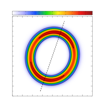
Figure 1: Image of the continuum emission at λobs=890μmsubscript𝜆obs890𝜇m\lambda_{\mathrm{obs}}=890\ \mu\mathrm{m} taken with ALMA. Black contours denote the intensity Iobs(Jyasec2)subscriptsuperscript𝐼obsJysuperscriptasec2I^{*}_{\mathrm{obs}}\ \left(\mathrm{Jy}\ \mathrm{asec^{-2}}\right) at log[Iobs]=2.0subscriptsuperscript𝐼obs2.0\log\left[I^{*}_{\mathrm{obs}}\right]=-2.0, 1.51.5-1.5, 1.01.0-1.0, 0.50.5-0.5, 0.00.00.0. The gray contours denote the intensity at 5σ5𝜎5\ \sigma level (1σ=0.61mJyasec21𝜎0.61mJysuperscriptasec21\ \sigma=0.61\ \mathrm{mJy\ asec^{-2}}). The synthesized beam is shown in the bottom left corner. The far side is in the northeast while the near side is in the southwest.
Table 1: Gaussian-fitted results for the observed radial intensity profiles.
PA𝑃superscript𝐴PA^{\prime} I0,obssubscriptsuperscript𝐼0obsI^{*}_{0,\mathrm{obs}} w0,obssubscriptsuperscript𝑤0obsw^{*}_{0,\mathrm{obs}} r0,obssubscriptsuperscript𝑟0obsr^{*}_{0,\mathrm{obs}}
(Jyasec2)Jysuperscriptasec2(\mathrm{Jy\ asec^{-2}}) (au)au(\mathrm{au}) (au)au(\mathrm{au})
1030superscript10superscript3010^{\circ}-30^{\circ} 1.161.161.16 50.950.950.9 158.4158.4158.4
3050superscript30superscript5030^{\circ}-50^{\circ} 1.251.251.25 51.051.051.0 152.3152.3152.3
5070superscript50superscript7050^{\circ}-70^{\circ} 1.191.191.19 50.250.250.2 148.6148.6148.6
7090superscript70superscript9070^{\circ}-90^{\circ} 0.940.940.94 49.049.049.0 143.1143.1143.1
90110superscript90superscript110\phantom{1}90^{\circ}-110^{\circ} 0.720.720.72 47.047.047.0 142.6142.6142.6
110130superscript110superscript130110^{\circ}-130^{\circ} 0.550.550.55 45.945.945.9 145.2145.2145.2
130150superscript130superscript150130^{\circ}-150^{\circ} 0.390.390.39 45.545.545.5 150.6150.6150.6
150170superscript150superscript170150^{\circ}-170^{\circ} 0.220.220.22 45.645.645.6 159.7159.7159.7
170190superscript170superscript190170^{\circ}-190^{\circ} 0.110.110.11 46.546.546.5 169.5169.5169.5
190210superscript190superscript210190^{\circ}-210^{\circ} 0.070.070.07 47.847.847.8 179.2179.2179.2
210230superscript210superscript230210^{\circ}-230^{\circ} 0.060.060.06 50.550.550.5 178.3178.3178.3
230250superscript230superscript250230^{\circ}-250^{\circ} 0.050.050.05 51.651.651.6 174.1174.1174.1
250270superscript250superscript270250^{\circ}-270^{\circ} 0.130.130.13 47.947.947.9 161.5161.5161.5
270290superscript270superscript290270^{\circ}-290^{\circ} 0.340.340.34 48.748.748.7 158.9158.9158.9
290310superscript290superscript310290^{\circ}-310^{\circ} 0.620.620.62 48.248.248.2 157.9157.9157.9
310330superscript310superscript330310^{\circ}-330^{\circ} 0.960.960.96 48.548.548.5 158.6158.6158.6
330350superscript330superscript350330^{\circ}-350^{\circ} 1.161.161.16 48.348.348.3 160.4160.4160.4
35010superscript350superscript10350^{\circ}-10^{\circ}\phantom{3} 1.131.131.13 49.349.349.3 159.9159.9159.9

Calibration and data reduction are made with the Common Astronomy Software Applications package version 3.4. We use Briggs weighting with a robust parameter of 0.50.50.5 during the self-calibration, in order to recover the weak and extended components of the dust emission (Muto et al., 2015). The synthesized beam (FWHM) is 0\farcs40×0\farcs470\farcs400\farcs470\farcs 40\times 0\farcs 47 (PA=59\fdg9𝑃𝐴59\fdg9PA=59\fdg 9), or 56au×66au56au66au56\ \mathrm{au}\times 66\ \mathrm{au} at the distance of HD 142527. The RMS noise level is 0.61mJyasec20.61mJysuperscriptasec20.61\ \mathrm{mJy\ asec^{-2}}. Figure 1 shows the self-calibrated image of the disk surrounding HD 142527.

As the groundwork in our modeling, we create radial intensity profiles of the continuum emission for 181818 azimuthal sectors with a radial bin width of 14au14au14\ \mathrm{au}. We fit these discrete averaged intensities in every sector by using a Gaussian function,

Iobssubscriptsuperscript𝐼obs\displaystyle I^{*}_{\mathrm{obs}} (robs)=I0,obsexp[(robsr0,obsw0,obs)2],subscriptsuperscript𝑟obssubscriptsuperscript𝐼0obssuperscriptsubscriptsuperscript𝑟obssubscriptsuperscript𝑟0obssubscriptsuperscript𝑤0obs2\displaystyle\left(r^{*}_{\mathrm{obs}}\right)=I^{*}_{0,\mathrm{obs}}\ \exp\left[-{\left(\frac{r^{*}_{\mathrm{obs}}-r^{*}_{0,\mathrm{obs}}}{w^{*}_{0,\mathrm{obs}}}\right)}^{2}\right], (1)

where robssubscriptsuperscript𝑟obsr^{*}_{\mathrm{obs}} denotes the projected radius from the star, I0,obssubscriptsuperscript𝐼0obsI^{*}_{0,\mathrm{obs}} the peak intensity at r0,obssubscriptsuperscript𝑟0obsr^{*}_{0,\mathrm{obs}}, and w0,obssubscriptsuperscript𝑤0obsw^{*}_{0,\mathrm{obs}} the projected width of the radial profile. The results of Gaussian-fitting are listed in table 1. In this paper, we use PA𝑃superscript𝐴PA^{\prime}, the angle measured from the disk major axis, to denote the azimuthal position of the disk instead of PA𝑃𝐴PA, i.e., PA=PA+19𝑃superscript𝐴𝑃𝐴superscript19PA^{\prime}=PA+19^{\circ}. Equation (1) is a function of PA𝑃superscript𝐴PA^{\prime}, but we have omitted it for convenience.

3 Modeling procedure
-101234-101234Refer to caption

log[κ/(1cm2g1)]𝜅1superscriptcm2superscriptg1\log\left[\kappa/\left(1\ \mathrm{cm^{2}\ g^{-1}}\right)\right]

log[λ/(1μm)]𝜆1𝜇m\log\left[\lambda/\left(1\ \mu\mathrm{m}\right)\right]
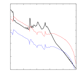
Figure 2: Conventional values of the absorption opacity (black solid line) and the scattering opacity (red dashed line) per unit dust mass, for compact dust grains following distribution a3.5superscript𝑎3.5a^{-3.5}, with amax=1mmsubscript𝑎max1mma_{\mathrm{max}}=1\ \mathrm{mm}. The blue dashed line indicates the scattering opacity reduced to 10%percent1010\% from their conventional values.
Refer to caption-2.0-1.5-1.0-0.50.00.51.01.52.0δR.A.(asec)formulae-sequence𝛿RAasec\delta\mathrm{R.A.}\ \left(\mathrm{asec}\right)-2.0-1.5-1.0-0.50.00.51.01.52.0

δDec.(asec)formulae-sequence𝛿Decasec\delta\mathrm{Dec.}\ \left(\mathrm{asec}\right)

0.000.020.040.060.080.100.12I(Jyasec2)superscript𝐼Jysuperscriptasec2I^{\prime}\ \left(\mathrm{Jy\ asec^{-2}}\right)(a)far sidenear sidemajor axisPA=0𝑃superscript𝐴superscript0PA^{\prime}=0^{\circ}
(a)
Refer to caption-2.0-1.5-1.0-0.50.00.51.01.52.0δR.A.(asec)formulae-sequence𝛿RAasec\delta\mathrm{R.A.}\ \left(\mathrm{asec}\right)-2.0-1.5-1.0-0.50.00.51.01.52.0

δDec.(asec)formulae-sequence𝛿Decasec\delta\mathrm{Dec.}\ \left(\mathrm{asec}\right)

0.000.501.001.502.00I(Jyasec2)superscript𝐼Jysuperscriptasec2I^{\prime}\ \left(\mathrm{Jy\ asec^{-2}}\right)(b)far sidenear sidemajor axisPA=0𝑃superscript𝐴superscript0PA^{\prime}=0^{\circ}
(b)
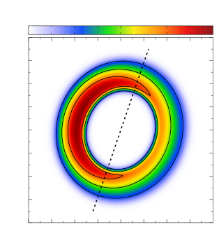
Figure 3: Disk intensity images obtained by ray-tracing simulation. Isuperscript𝐼I^{\prime} is the intensity before beam convolution. The dashed line indicates the major axis of the disk along PA=0𝑃superscript𝐴superscript0PA^{\prime}=0^{\circ}. The simulated images are based on w0=27ausubscript𝑤027auw_{0}=27\ \mathrm{au} and r0=175ausubscript𝑟0175aur_{0}=175\ \mathrm{au} models. (a): Σ0=0.01gcm2subscriptΣ00.01gsuperscriptcm2\Sigma_{0}=0.01\ \mathrm{g\ cm^{-2}} model. The contours are drawn at I=0.02superscript𝐼0.02I^{\prime}=0.02, 0.060.060.06, 0.10Jyasec20.10Jysuperscriptasec20.10\ \mathrm{Jy\ asec^{-2}}. (b): Σ0=1.00gcm2subscriptΣ01.00gsuperscriptcm2\Sigma_{0}=1.00\ \mathrm{g\ cm^{-2}} model. The contours are drawn at I=0.50superscript𝐼0.50I^{\prime}=0.50, 1.001.001.00, 1.50Jyasec21.50Jysuperscriptasec21.50\ \mathrm{Jy\ asec^{-2}}.

Our goal is to derive the dust surface density distribution for the disk that reproduces I0,obssubscriptsuperscript𝐼0obsI^{*}_{0,\mathrm{obs}}, w0,obssubscriptsuperscript𝑤0obsw^{*}_{0,\mathrm{obs}}, and r0,obssubscriptsuperscript𝑟0obsr^{*}_{0,\mathrm{obs}} in each PA𝑃superscript𝐴PA^{\prime} sector. Since the observed intensity of the disk around HD 142527 varies smoothly in the azimuthal direction, we employ a 2D axisymmetric model as a fiducial model to reproduce the intensity in each sector individually (Muto et al. 2015). The scattered light of the observed crescent disk, however, may be different from that of the axisymmetric model when scattering is dominant; the validity of this approach is discussed in Section 5.2.

The dust surface density distribution in the radial (r𝑟r) direction is assumed to be

Σ(r)=Σ0exp{min[(rr0w0)2, 20]},Σ𝑟subscriptΣ0minsuperscript𝑟subscript𝑟0subscript𝑤0220\displaystyle\Sigma\left(r\right)=\Sigma_{0}\ \exp\left\{-\mathrm{min}\left[{\left(\frac{r-r_{0}}{w_{0}}\right)}^{2},\ 20\right]\right\}, (2)

where Σ0subscriptΣ0\Sigma_{0}, w0subscript𝑤0w_{0}, and r0subscript𝑟0r_{0} denote the peak surface density, the radial width of the distribution, and the peak radius, respectively. Note that the floor exp(20)20\exp{(-20)} is set for computational convenience. We determine (Σ0,w0,r0)subscriptΣ0subscript𝑤0subscript𝑟0(\Sigma_{0},w_{0},r_{0}) by the following procedure:

  1. 1.

    Compute the surface density distribution, Σ(r)Σ𝑟\Sigma(r), for given sets of (Σ0,w0,r0)subscriptΣ0subscript𝑤0subscript𝑟0(\Sigma_{0},w_{0},r_{0}). The model parameters are varied in the range of 2.1logΣ0(gcm2)0.12.1subscriptΣ0gsuperscriptcm20.1-2.1\leq\log\Sigma_{0}~{}(\mathrm{g~{}cm^{-2}})\leq 0.1 with the interval ΔlogΣ0=0.1ΔsubscriptΣ00.1\Delta\log\Sigma_{0}=0.1, in 21auw031au21ausubscript𝑤031au21~{}\mathrm{au}\leq w_{0}\leq 31~{}\mathrm{au} with Δw0=2auΔsubscript𝑤02au\Delta w_{0}=2~{}\mathrm{au}, and in 159aur0199au159ausubscript𝑟0199au159~{}\mathrm{au}\leq r_{0}\leq 199~{}\mathrm{au} with Δr0=8auΔsubscript𝑟08au\Delta r_{0}=8~{}\mathrm{au}. They are extended slightly when necessary.

  2. 2.

    Calculate the density ρ(r,z)𝜌𝑟𝑧\rho\left(r,z\right), temperature T(r,z)𝑇𝑟𝑧T\left(r,z\right), and mean intensity Jν(r,z)subscript𝐽𝜈𝑟𝑧J_{\nu}\left(r,z\right) for each (Σ0,w0,r0)subscriptΣ0subscript𝑤0subscript𝑟0(\Sigma_{0},w_{0},r_{0}) by assuming the radiative and hydrostatic equilibria (Section 3.2).

  3. 3.

    Calculate model intensity by ray-tracing, and extract the radial profiles after convolving the image with the synthesized beam of the observation (Section 3.3).

  4. 4.

    Fit the radial profiles of the model intensity with the Gaussian function and obtain their (I0,w0,r0)subscriptsuperscript𝐼0subscriptsuperscript𝑤0subscriptsuperscript𝑟0(I^{*}_{0},w^{*}_{0},r^{*}_{0}) of the model, which are compared with (I0,obs,w0,obs,r0,obs)subscriptsuperscript𝐼0obssubscriptsuperscript𝑤0obssubscriptsuperscript𝑟0obs(I^{*}_{0,\mathrm{obs}},w^{*}_{0,\mathrm{obs}},r^{*}_{0,\mathrm{obs}}) in the same PA𝑃superscript𝐴PA^{\prime} sector (Section 3.4). Search for parameters (Σ0,r0,w0)subscriptΣ0subscript𝑟0subscript𝑤0(\Sigma_{0},r_{0},w_{0}) that meet the criteria in equation (3.4). If necessary, construct a refined model by interpolating Σ0subscriptΣ0\Sigma_{0} and r0subscript𝑟0r_{0}.

In the following, we explain the procedure in detail.

3.1 Assumptions on dust properties

We assume a dust grain in the disk to be a compact sphere composed of silicate, carbonaceous compounds, and water ice; their mass fractional abundances relative to the hydrogen mass are taken to be 0.00430.00430.0043, 0.00300.00300.0030, and 0.00940.00940.0094, respectively, which are consistent with the solar elemental abundance (Anders & Grevesse, 1989). The grains have a power-law size distribution,

dn(a)daa3.5,amax=1mm,formulae-sequenceproportional-to𝑑𝑛𝑎𝑑𝑎superscript𝑎3.5subscript𝑎max1mm\displaystyle\frac{dn(a)}{da}\propto a^{-3.5},\ a_{\mathrm{max}}=1\mathrm{\ mm}, (3)

where a𝑎a and amaxsubscript𝑎maxa_{\mathrm{max}} denote the grain radius and the maximum grain radius, respectively. The choice of amaxsubscript𝑎maxa_{\mathrm{max}} is based on the observed spectral opacity index, β1similar-to𝛽1\beta\sim 1 (Verhoeff et al., 2011). The absorption and scattering cross sections, Ca(a)subscript𝐶a𝑎C_{\mathrm{a}}(a) and Cs(a)subscript𝐶s𝑎C_{\mathrm{s}}(a), and the asymmetry parameter g(a)𝑔𝑎g(a) 111The asymmetry parameter describes the anisotropy in scattering and takes value within |g|1𝑔1|g|\leq 1 (see, e.g., Bohren & Huffman (1983)). For symmetric scattering about the axis perpendicular to the propagation direction of incident wave, g=0𝑔0g=0. If the grain tends to scatter light toward the forward (backward) direction, g𝑔g is positive (negative). for every grain size in the power-law distribution are calculated using Mie theory. The scattering cross section and its asymmetry parameter are defined as

Cs(a)=4πdCs(a)dΩ𝑑Ωsubscript𝐶s𝑎subscript4𝜋𝑑subscript𝐶s𝑎𝑑Ωdifferential-dΩ\displaystyle C_{\mathrm{s}}(a)=\int_{4\pi}\frac{dC_{\mathrm{s}}(a)}{d\Omega}d\Omega (4)

and

g(a)=1Cs(a)4πdCs(a)dΩcosΘ(a)𝑑Ω,𝑔𝑎1subscript𝐶s𝑎subscript4𝜋𝑑subscript𝐶s𝑎𝑑ΩΘ𝑎differential-dΩ\displaystyle g(a)=\frac{1}{C_{\mathrm{s}}(a)}\int_{4\pi}\frac{dC_{\mathrm{s}}(a)}{d\Omega}\cos\Theta(a)d\Omega, (5)

respectively, where dCs(a)/dΩ𝑑subscript𝐶s𝑎𝑑ΩdC_{\mathrm{s}}(a)/d\Omega is the differential scattering cross section and Θ(a)Θ𝑎\Theta(a) the deflection angle from the propagation direction Θ(a)=0Θ𝑎superscript0\Theta(a)=0^{\circ}. To take into account the effects of asymmetric scattering in the M1 model (see Appendix A for more details), we incorporate the asymmetry parameter by multiplying Cs(a)subscript𝐶s𝑎C_{\mathrm{s}}(a) by [1g(a)]delimited-[]1𝑔𝑎[1-g(a)]; the light scattered away from the propagation direction is treated as extinction along Θ=0Θsuperscript0\Theta=0^{\circ}. In this way, the effects of self-scattering are considered while keeping the computational time for radiative transfer reasonable. Denoting the grain mass by m(a)𝑚𝑎m(a), the scattering opacity used in this study is then defined as

κssubscript𝜅s\displaystyle\kappa_{\mathrm{s}} =\displaystyle= {Cs(a)m(a)[1g(a)]}dn(a)da𝑑a,subscript𝐶s𝑎𝑚𝑎delimited-[]1𝑔𝑎𝑑𝑛𝑎𝑑𝑎differential-d𝑎\displaystyle\int\left\{\frac{C_{\mathrm{s}}(a)}{m(a)}\left[1-g(a)\right]\right\}\frac{dn(a)}{da}da, (6)

which is weighted by the size distribution. Similarly, dividing Ca(a)subscript𝐶a𝑎C_{\mathrm{a}}(a) by m(a)𝑚𝑎m(a) and integrate over the size distribution we obtain the absorption opacity as

κasubscript𝜅a\displaystyle\kappa_{\mathrm{a}} =\displaystyle= {Ca(a)m(a)}dn(a)da𝑑a.subscript𝐶a𝑎𝑚𝑎𝑑𝑛𝑎𝑑𝑎differential-d𝑎\displaystyle\int\left\{\frac{C_{\mathrm{a}}(a)}{m(a)}\right\}\frac{dn(a)}{da}da. (7)

The opacities are shown in figure 2. When amaxsubscript𝑎maxa_{\mathrm{max}} is comparable to λobssubscript𝜆obs\lambda_{\mathrm{obs}}, κssubscript𝜅s\kappa_{\mathrm{s}} is larger than κasubscript𝜅a\kappa_{\mathrm{a}} by a factor of about 101010; κa=2.9cm2g1subscript𝜅a2.9superscriptcm2superscriptg1\kappa_{\mathrm{a}}=2.9\mathrm{\ cm^{2}\ g^{-1}} and κs=26.2cm2g1subscript𝜅s26.2superscriptcm2superscriptg1\kappa_{\mathrm{s}}=26.2\mathrm{\ cm^{2}\ g^{-1}} at λobs=890μmsubscript𝜆obs890𝜇m\lambda_{\mathrm{obs}}=890\mathrm{\ \mu m} (Aikawa & Nomura, 2006). As will be described in Section 5.1, we also use model where κssubscript𝜅s\kappa_{\mathrm{s}} is reduced by 90%percent9090\% from the conventional value.

3.2 Disk models

Applying the dust properties and the dust distribution, we solve the radiative transfer of the disk by the M1 model (González et al. (2007); Kanno et al. (2013); see also Appendix A). The 2D distributions of the dust density ρ(r,z)𝜌𝑟𝑧\rho(r,z), the temperature T(r,z)𝑇𝑟𝑧T(r,z), and the mean intensity Jν(r,z)subscript𝐽𝜈𝑟𝑧J_{\nu}(r,z) are determined by the same method as Muto et al. (2015). We consider the star as the heat source and use 226226226 colors in 0.1μmλ3.16mm0.1𝜇m𝜆3.16mm0.1\ \mu\mathrm{m}\leq\lambda\leq 3.16\ \mathrm{mm} (spectral resolution of Δlogλ=0.02Δ𝜆0.02\Delta\log\lambda=0.02) to calculate the radiative and hydrostatic equilibria. In the cylindrical coordinates (r,φ,z)𝑟𝜑𝑧(r,\varphi,z), the star is located at the origin, while the disk is assumed to be axisymmetric around the z𝑧z-axis and reflection symmetric with respect to the midplane (z=0𝑧0z=0). The computation region covers 30aur410au30au𝑟410au30\ \mathrm{au}\leq r\leq 410\ \mathrm{au} and 0auz120au0au𝑧120au0\ \mathrm{au}\leq z\leq 120\ \mathrm{au} with a spatial resolution of 2au2au2\ \mathrm{au}. We did not take the effects of accretion into account. We also did not consider the shadows cast by the inner warped disk discussed by Marino et al. (2015).

3.3 Model Image

The emergent intensity of the model is calculated by ray-tracing along the line of sight zsuperscript𝑧z^{\prime}:

dIdz=(κa+κs)ρ(ISν),𝑑superscript𝐼𝑑superscript𝑧subscript𝜅asubscript𝜅s𝜌superscript𝐼subscript𝑆𝜈\displaystyle\frac{dI^{\prime}}{dz^{\prime}}=-(\kappa_{\mathrm{a}}+\kappa_{\mathrm{s}})\rho\left(I^{\prime}-S_{\nu}\right), (8)

where the source function is given by

Sνsubscript𝑆𝜈\displaystyle S_{\nu} =\displaystyle= (1η)Bν(T)+ηJν.1𝜂subscript𝐵𝜈𝑇𝜂subscript𝐽𝜈\displaystyle\left(1-\eta\right)B_{\nu}\left(T\right)+\eta J_{\nu}. (9)

The source function is the sum of the Planck function Bν(T)subscript𝐵𝜈𝑇B_{\nu}\left(T\right) and the angular-averaged intensity Jνsubscript𝐽𝜈J_{\nu}, each weighted by (1η)1𝜂(1-\eta) and η𝜂\eta, where

ηκsκa+κs,𝜂subscript𝜅ssubscript𝜅asubscript𝜅s\displaystyle\eta\equiv\frac{\kappa_{\mathrm{s}}}{\kappa_{\mathrm{a}}+\kappa_{\mathrm{s}}}, (10)

is the albedo. We obtain intensity distribution on the uniform grid of 2au2au2\ \mathrm{au} on the sky plane to construct the model image.

Figure 3 shows the intensity images obtained by ray-tracing for two peak surface density models, Σ0=0.01gcm2subscriptΣ00.01gsuperscriptcm2\Sigma_{0}=0.01\ \mathrm{g\ cm^{-2}} and 1.00gcm21.00gsuperscriptcm21.00\ \mathrm{g\ cm^{-2}}, with w0=27ausubscript𝑤027auw_{0}=27\ \mathrm{au}, r0=175ausubscript𝑟0175aur_{0}=175\ \mathrm{au}, and i=27𝑖superscript27i=27^{\circ}. The former represents an optically thin disk, while the latter represents an optically thick disk. In the following, the coordinates of the disk projected in the sky are denoted by (r,PA)superscript𝑟𝑃superscript𝐴(r^{\prime},PA^{\prime}), i.e., coordinates with primes (). The regions of 0<PA<180superscript0𝑃superscript𝐴superscript1800^{\circ}<PA^{\prime}<180^{\circ} and 180<PA<360superscript180𝑃superscript𝐴superscript360180^{\circ}<PA^{\prime}<360^{\circ} correspond to the far side and the near side, respectively. The disk images appear slightly elongated in the major axis (PA=0𝑃superscript𝐴superscript0PA^{\prime}=0^{\circ}) because of the disk inclination, but they are reflection symmetry with respect to the minor axis (PA=90𝑃superscript𝐴superscript90PA^{\prime}=90^{\circ}). The intensity depends on PA𝑃superscript𝐴PA^{\prime} although the model is axisymmetric. It is highest on the major axis in the optically thin disk (figure 3a), but on the far side in the optically thick disk (figure 3b). When the disk is optically thin, the intensity is roughly proportional to the amount of dust along the line of sight. The major axis is brightest since the line of sight intersects the disk plane longer. When the disk is optically thick, the hot inner wall facing the star is exposed to us on the far side, thus its intensity is higher than that on the near side where the wall is hidden from sight. We take this PA𝑃superscript𝐴PA^{\prime} dependence into account in our analysis.

The next step is the convolution of the above images with a Gaussian beam to mimic the observation. Physical quantities obtained after beam convolution are indicated with asterisks (). Since the beam is elliptical with its major axis lying along PA=78.9𝑃superscript𝐴superscript78.9PA^{\prime}=78.9^{\circ}, the image no longer retains its reflection symmetry with respect to the minor axis after the beam convolution. We then extract the radial intensity profiles from the convolved image and fit them with Gaussian function to obtain I0subscriptsuperscript𝐼0I^{*}_{0}, w0subscriptsuperscript𝑤0w^{*}_{0}, and r0subscriptsuperscript𝑟0r^{*}_{0}.

3.4 Comparison between observation and simulation

For each sector, a parameter cube (I0,w0,r0)subscriptsuperscript𝐼0subscriptsuperscript𝑤0subscriptsuperscript𝑟0(I^{*}_{0},w^{*}_{0},r^{*}_{0}) associated with (Σ0,w0,r0)subscriptΣ0subscript𝑤0subscript𝑟0(\Sigma_{0},w_{0},r_{0}) is created. The best fit parameters for the dust distribution are searched by comparing the Gaussian-fitted values between the model and the observation. The best fit model should satisfy the following criteria: {subeqnarray} — ΔI^*_0 — &≡ — I^*_0,obs - I^*_0 — ≤0.01 I^*_0,obs,
— Δw^*_0 — ≡ —w^*_0,obs - w^*_0 — ≤1 au,
— Δr^*_0 — ≡ —r^*_0,obs - r^*_0 — ≤1 au. In order to discern the trend in the PA𝑃superscript𝐴PA^{\prime} direction, criteria better than the beam resolution are set. These criteria are different from those of Muto et al. (2015), who placed a ±10%plus-or-minuspercent10\pm 10\% tolerance for all the criteria above.

To facilitate the parameter search for the dust distribution and to save the computational time, we interpolate models to complement our sample on Σ0subscriptΣ0\Sigma_{0} and r0subscript𝑟0r_{0}. The interpolation among four adjacent (Σ0,w0,r0)subscriptΣ0subscript𝑤0subscript𝑟0(\Sigma_{0},w_{0},r_{0}) models at (r,z)𝑟𝑧(r,z) is carried out by the following weighted average:

A𝐴\displaystyle A (r,z;Σ0,i,w0,r0,i)=𝑟𝑧subscriptΣ0isubscript𝑤0subscript𝑟0iabsent\displaystyle\left(r,z;\Sigma_{0,\mathrm{i}},w_{0},r_{0,\mathrm{i}}\right)= (11)
n=12ln[m=12kmA(r+r0,mr0,i,z;Σ0,n,w0,r0,m)],superscriptsubscript𝑛12subscript𝑙𝑛delimited-[]superscriptsubscript𝑚12subscript𝑘𝑚𝐴𝑟subscript𝑟0𝑚subscript𝑟0i𝑧subscriptΣ0𝑛subscript𝑤0subscript𝑟0𝑚\displaystyle\sum\limits_{n=1}^{2}l_{n}\left[\sum\limits_{m=1}^{2}k_{m}A\left(r+r_{0,m}-r_{0,\mathrm{i}},z;\Sigma_{0,n},w_{0},r_{0,m}\right)\right],

where A𝐴A represents ρ𝜌\rho, T𝑇T, or Jνsubscript𝐽𝜈J_{\nu}. The weighting factors fmsubscript𝑓𝑚f_{m} and gnsubscript𝑔𝑛g_{n} are defined as

k1subscript𝑘1\displaystyle k_{1} =\displaystyle= 1|r0,ir0,1r0,2r0,1|1subscript𝑟0isubscript𝑟01subscript𝑟02subscript𝑟01\displaystyle 1-\left|\frac{r_{0,\mathrm{i}}-r_{0,1}}{r_{0,2}-r_{0,1}}\right|
k2subscript𝑘2\displaystyle k_{2} =\displaystyle= 1k11subscript𝑘1\displaystyle 1-k_{1}
l1subscript𝑙1\displaystyle l_{1} =\displaystyle= 1|Σ0,iΣ0,1Σ0,2Σ0,1|1subscriptΣ0isubscriptΣ01subscriptΣ02subscriptΣ01\displaystyle 1-\left|\frac{\Sigma_{0,\mathrm{i}}-\Sigma_{0,1}}{\Sigma_{0,2}-\Sigma_{0,1}}\right|
l2subscript𝑙2\displaystyle l_{2} =\displaystyle= 1l11subscript𝑙1\displaystyle 1-l_{1}

The subscripts “111” and “222” specify the two existing models, while the subscript “ii\mathrm{i}” specifies the interpolated product. We do not perform interpolation on w0subscript𝑤0w_{0} because its 222-auau\mathrm{au} interval in the parameter space is sufficiently refined to fulfill equation (3.4b).

4 Results

Table 2: Derived best fit values using the conventional model for dust opacity.
PA𝑃superscript𝐴PA^{\prime} Σ0subscriptΣ0\Sigma_{0} w0subscript𝑤0w_{0} r0subscript𝑟0r_{0} Msecsubscript𝑀secM_{\mathrm{sec}} ΔI0Δsubscriptsuperscript𝐼0\Delta I^{*}_{0} Δw0Δsubscriptsuperscript𝑤0\Delta w^{*}_{0} Δr0Δsubscriptsuperscript𝑟0\Delta r^{*}_{0}
(gcm2)gsuperscriptcm2\left(\mathrm{g\ cm^{-2}}\right) (au)au\left(\mathrm{au}\right) (au)au\left(\mathrm{au}\right) (M)subscript𝑀direct-product\left(M_{\odot}\right) (×I0,obs)\left(\times I^{*}_{0,\mathrm{obs}}\right) (au)au\left(\mathrm{au}\right) (au)au\left(\mathrm{au}\right)
1030superscript10superscript3010^{\circ}-30^{\circ} 7.89×1017.89superscript1017.89\times 10^{-1} 232323 175175175 2.1×1042.1superscript1042.1\times 10^{-4} 1.3×1051.3superscript105-1.3\times 10^{-5} +0.80.8+0.8 0.50.5-0.5
3050superscript30superscript5030^{\circ}-50^{\circ} 1.121.121.12 212121 173173173 2.6×1042.6superscript1042.6\times 10^{-4} 2.9×1052.9superscript105-2.9\times 10^{-5} +0.30.3+0.3 0.30.3-0.3
5070superscript50superscript7050^{\circ}-70^{\circ} 7.28×1017.28superscript1017.28\times 10^{-1} 212121 173173173 1.5×1041.5superscript1041.5\times 10^{-4} 1.0×1051.0superscript105-1.0\times 10^{-5} 0.30.3-0.3 0.50.5-0.5
7090superscript70superscript9070^{\circ}-90^{\circ} 3.07×1013.07superscript1013.07\times 10^{-1} 212121 167167167 5.9×1055.9superscript1055.9\times 10^{-5} 2.5×1052.5superscript105-2.5\times 10^{-5} +0.10.1+0.1 0.30.3-0.3
90110superscript90superscript110\phantom{1}90^{\circ}-110^{\circ} 2.00×1012.00superscript1012.00\times 10^{-1} 212121 165165165 3.8×1053.8superscript1053.8\times 10^{-5} 4.0×1054.0superscript105-4.0\times 10^{-5} 0.40.4-0.4 +0.80.8+0.8
110130superscript110superscript130110^{\circ}-130^{\circ} 1.33×1011.33superscript1011.33\times 10^{-1} 232323 165165165 2.7×1052.7superscript1052.7\times 10^{-5} 1.6×1051.6superscript105-1.6\times 10^{-5} 0.20.2-0.2 0.10.1-0.1
130150superscript130superscript150130^{\circ}-150^{\circ} 7.83×1027.83superscript1027.83\times 10^{-2} 232323 165165165 1.9×1051.9superscript1051.9\times 10^{-5} 4.0×1054.0superscript105-4.0\times 10^{-5} +0.40.4+0.4 +0.60.6+0.6
150170superscript150superscript170150^{\circ}-170^{\circ} 3.61×1023.61superscript1023.61\times 10^{-2} 272727 171171171 1.1×1051.1superscript1051.1\times 10^{-5} 1.1×1051.1superscript105-1.1\times 10^{-5} +0.20.2+0.2 0.80.8-0.8
170190superscript170superscript190170^{\circ}-190^{\circ} 1.61×1021.61superscript1021.61\times 10^{-2} 292929 177177177 5.7×1065.7superscript1065.7\times 10^{-6} 4.3×1054.3superscript105-4.3\times 10^{-5} +0.50.5+0.5 0.00.0-0.0
190210superscript190superscript210190^{\circ}-210^{\circ} 1.10×1021.10superscript1021.10\times 10^{-2} 292929 189189189 4.1×1064.1superscript1064.1\times 10^{-6} 4.5×1054.5superscript105-4.5\times 10^{-5} +0.50.5+0.5 0.60.6-0.6
210230superscript210superscript230210^{\circ}-230^{\circ} 9.05×1039.05superscript1039.05\times 10^{-3} 323232 193193193 3.5×1063.5superscript1063.5\times 10^{-6} 1.3×1051.3superscript105-1.3\times 10^{-5} 0.70.7-0.7 +0.70.7+0.7
230250superscript230superscript250230^{\circ}-250^{\circ} 8.31×1038.31superscript1038.31\times 10^{-3} 323232 195195195 3.0×1063.0superscript1063.0\times 10^{-6} 4.6×1054.6superscript105-4.6\times 10^{-5} 0.70.7-0.7 +0.80.8+0.8
250270superscript250superscript270250^{\circ}-270^{\circ} 2.89×1022.89superscript1022.89\times 10^{-2} 232323 185185185 6.8×1066.8superscript1066.8\times 10^{-6} 1.7×1051.7superscript105-1.7\times 10^{-5} 0.40.4-0.4 +0.10.1+0.1
270290superscript270superscript290270^{\circ}-290^{\circ} 8.60×1028.60superscript1028.60\times 10^{-2} 232323 183183183 2.0×1052.0superscript1052.0\times 10^{-5} 3.6×1053.6superscript105-3.6\times 10^{-5} +0.20.2+0.2 0.00.0-0.0
290310superscript290superscript310290^{\circ}-310^{\circ} 2.21×1012.21superscript1012.21\times 10^{-1} 232323 179179179 4.9×1054.9superscript1054.9\times 10^{-5} 1.5×1051.5superscript105-1.5\times 10^{-5} +0.30.3+0.3 +0.10.1+0.1
∗*∗*footnotemark: *310330superscript310superscript330310^{\circ}-330^{\circ} 1.261.261.26 212121 179179179 3.0×1043.0superscript1043.0\times 10^{-4} (5.7×10²)5.7superscript102(-5.7\times 10^{-2}) (2.9)2.9(-2.9) +0.90.9+0.9
∗*∗*footnotemark: *330350superscript330superscript350330^{\circ}-350^{\circ} 1.261.261.26 212121 177177177 3.2×1043.2superscript1043.2\times 10^{-4} (1.6×101)1.6superscript101(-1.6\times 10^{-1}) (1.2)1.2(-1.2) 0.40.4-0.4
∗*∗*footnotemark: *35010superscript350superscript10350^{\circ}-10^{\circ}\phantom{3} 1.261.261.26 212121 173173173 3.2×1043.2superscript1043.2\times 10^{-4} (3.4×10²)3.4superscript102(-3.4\times 10^{-2}) +0.70.7+0.7 +1.01.0+1.0
{tabnote}∗*∗*footnotemark: *

PA=310330𝑃superscript𝐴superscript310superscript330PA^{\prime}=310^{\circ}-330^{\circ}, PA=330350𝑃superscript𝐴superscript330superscript350PA^{\prime}=330^{\circ}-350^{\circ}, and PA=35010𝑃superscript𝐴superscript350superscript10PA^{\prime}=350^{\circ}-10^{\circ} are failed to be reproduced using the conventional model. The parenthesized parameters are those that do not fulfill the criteria in equation (3.4).

4.1 Derived best fit values

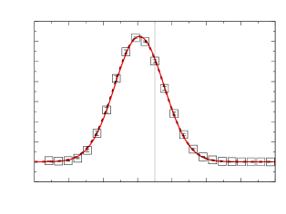
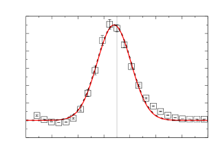
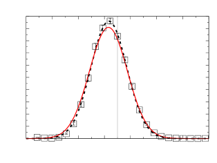
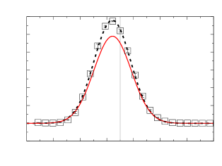
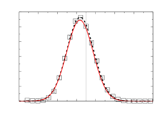
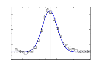
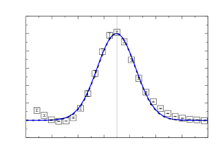
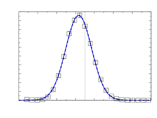
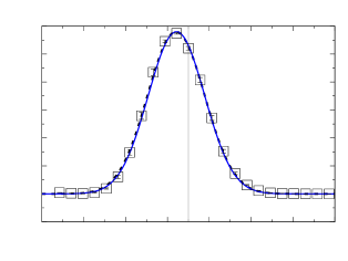
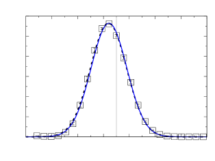
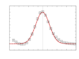
Figure 4 shows the results of the model fitting for all PA𝑃superscript𝐴PA^{\prime} sectors. The 151515 radial profiles in PA=10310𝑃superscript𝐴superscript10superscript310PA^{\prime}=10^{\circ}-310^{\circ} are well reproduced by the models; their parameters are listed in table 2. The mass contained in each PA𝑃superscript𝐴PA^{\prime} sector, Msecsubscript𝑀secM_{\mathrm{sec}}, is also presented. However, none of the models succeed in reproducing the three radial profiles in PA=31010𝑃superscript𝐴superscript310superscript10PA^{\prime}=310^{\circ}-10^{\circ} (figure 4d, 4e, and 4f). These three sectors will be described separately in Section 4.2.

We derived Σ0=1.12gcm2subscriptΣ01.12gsuperscriptcm2\Sigma_{0}=1.12\ \mathrm{g\ cm^{-2}} for the brightest PA=3050𝑃superscript𝐴superscript30superscript50PA^{\prime}=30^{\circ}-50^{\circ}, and Σ0=8.31×10³gcm2subscriptΣ08.31superscript103gsuperscriptcm2\Sigma_{0}=8.31\times 10^{-3}\ \mathrm{g\ cm^{-2}} for the faintest PA=230250𝑃superscript𝐴superscript230superscript250PA^{\prime}=230^{\circ}-250^{\circ}. The contrast in Σ0subscriptΣ0\Sigma_{0} between these two sectors is about a factor of 130130130, which is twice the value derived by Muto et al. (2015). The apparent discrepancy is discussed in Section 4.3. Our model might overestimate the temperature in the north (PA11𝑃superscript𝐴superscript11PA^{\prime}\approx 11^{\circ}) and the south (PA191𝑃superscript𝐴superscript191PA^{\prime}\approx 191^{\circ}) of the outer disk, as we did not consider the possible shadowing effects caused by the warped inner disk (Marino et al., 2015; Casassus et al., 2015). As a consequence, the best fit Σ0subscriptΣ0\Sigma_{0} for PA=35010𝑃superscript𝐴superscript350superscript10PA^{\prime}=350^{\circ}-10^{\circ} and PA=150170𝑃superscript𝐴superscript150superscript170PA^{\prime}=150^{\circ}-170^{\circ} might be considered as lower limits.
-0.200.000.200.400.600.801.001.201.40050100150200250300350Σ0=1.12gcm2subscriptΣ01.12gsuperscriptcm2\Sigma_{0}=1.12\ \mathrm{g\ cm^{-2}}w0=21ausubscript𝑤021auw_{0}=21\ \mathrm{au}r0=173ausubscript𝑟0173aur_{0}=173\ \mathrm{au}Msec=2.6×10⁴Msubscript𝑀sec2.6superscript104subscript𝑀direct-productM_{\mathrm{sec}}=2.6\times 10^{-4}\ M_{\odot}Refer to caption

I(Jyasec2)superscript𝐼Jysuperscriptasec2I^{*}\left(\mathrm{Jy\ asec^{-2}}\right)

r(au)superscript𝑟aur^{*}\left(\mathrm{au}\right)PA=3050𝑃superscript𝐴superscript30superscript50PA^{\prime}=30^{\circ}-50^{\circ}
(a)
-0.020.000.020.040.060.080.100.12050100150200250300350Σ0=1.61×10²gcm2subscriptΣ01.61superscript102gsuperscriptcm2\Sigma_{0}=1.61\times 10^{-2}\ \mathrm{g\ cm^{-2}}w0=29ausubscript𝑤029auw_{0}=29\ \mathrm{au}r0=177ausubscript𝑟0177aur_{0}=177\ \mathrm{au}Msec=5.7×10⁶Msubscript𝑀sec5.7superscript106subscript𝑀direct-productM_{\mathrm{sec}}=5.7\times 10^{-6}\ M_{\odot}Refer to caption

I(Jyasec2)superscript𝐼Jysuperscriptasec2I^{*}\left(\mathrm{Jy\ asec^{-2}}\right)

r(au)superscript𝑟aur^{*}\left(\mathrm{au}\right)PA=170190𝑃superscript𝐴superscript170superscript190PA^{\prime}=170^{\circ}-190^{\circ}
(b)
-0.010.000.010.020.030.040.050.06050100150200250300350Σ0=8.85×10³gcm2subscriptΣ08.85superscript103gsuperscriptcm2\Sigma_{0}=8.85\times 10^{-3}\ \mathrm{g\ cm^{-2}}w0=29ausubscript𝑤029auw_{0}=29\ \mathrm{au}r0=195ausubscript𝑟0195aur_{0}=195\ \mathrm{au}Msec=2.9×10⁶Msubscript𝑀sec2.9superscript106subscript𝑀direct-productM_{\mathrm{sec}}=2.9\times 10^{-6}\ M_{\odot}Refer to caption

I(Jyasec2)superscript𝐼Jysuperscriptasec2I^{*}\left(\mathrm{Jy\ asec^{-2}}\right)

r(au)superscript𝑟aur^{*}\left(\mathrm{au}\right)PA=230250𝑃superscript𝐴superscript230superscript250PA^{\prime}=230^{\circ}-250^{\circ}
(c)
0.000.100.200.300.400.500.600.700.800.901.00050100150200250300350Σ0=1.26gcm2subscriptΣ01.26gsuperscriptcm2\Sigma_{0}=1.26\ \mathrm{g\ cm^{-2}}w0=21ausubscript𝑤021auw_{0}=21\ \mathrm{au}r0=179ausubscript𝑟0179aur_{0}=179\ \mathrm{au}Msec=3.0×10⁴Msubscript𝑀sec3.0superscript104subscript𝑀direct-productM_{\mathrm{sec}}=3.0\times 10^{-4}\ M_{\odot}Refer to caption

I(Jyasec2)superscript𝐼Jysuperscriptasec2I^{*}\left(\mathrm{Jy\ asec^{-2}}\right)

r(au)superscript𝑟aur^{*}\left(\mathrm{au}\right)PA=310330𝑃superscript𝐴superscript310superscript330PA^{\prime}=310^{\circ}-330^{\circ}
(d)
-0.200.000.200.400.600.801.001.20050100150200250300350Σ0=1.26gcm2subscriptΣ01.26gsuperscriptcm2\Sigma_{0}=1.26\ \mathrm{g\ cm^{-2}}w0=21ausubscript𝑤021auw_{0}=21\ \mathrm{au}r0=177ausubscript𝑟0177aur_{0}=177\ \mathrm{au}Msec=3.2×10⁴Msubscript𝑀sec3.2superscript104subscript𝑀direct-productM_{\mathrm{sec}}=3.2\times 10^{-4}\ M_{\odot}Refer to caption

I(Jyasec2)superscript𝐼Jysuperscriptasec2I^{*}\left(\mathrm{Jy\ asec^{-2}}\right)

r(au)superscript𝑟aur^{*}\left(\mathrm{au}\right)PA=330350𝑃superscript𝐴superscript330superscript350PA^{\prime}=330^{\circ}-350^{\circ}
(e)
0.000.200.400.600.801.001.20050100150200250300350Σ0=1.26gcm2subscriptΣ01.26gsuperscriptcm2\Sigma_{0}=1.26\ \mathrm{g\ cm^{-2}}w0=21ausubscript𝑤021auw_{0}=21\ \mathrm{au}r0=173ausubscript𝑟0173aur_{0}=173\ \mathrm{au}Msec=3.2×10⁴Msubscript𝑀sec3.2superscript104subscript𝑀direct-productM_{\mathrm{sec}}=3.2\times 10^{-4}\ M_{\odot}Refer to caption

I(Jyasec2)superscript𝐼Jysuperscriptasec2I^{*}\left(\mathrm{Jy\ asec^{-2}}\right)

r(au)superscript𝑟aur^{*}\left(\mathrm{au}\right)PA=35010𝑃superscript𝐴superscript350superscript10PA^{\prime}=350^{\circ}-10^{\circ}
(f)
Figure 4: The observed radial intensity profiles (plotted in square boxes with error bars in the Iobssubscriptsuperscript𝐼obsI^{*}_{\mathrm{obs}} direction) at λobs=890μmsubscript𝜆obs890𝜇m\lambda_{\mathrm{obs}}=890\ \mu\mathrm{m} of six PA𝑃superscript𝐴PA^{\prime} sectors as examples. Black dashed lines are Gaussian-fitted curves for the observational data points. The faint gray line at r=175ausuperscript𝑟175aur^{*}=175\ \mathrm{au} is drawn to emphasize the relative position of I0,obssubscriptsuperscript𝐼0obsI^{*}_{0,\mathrm{obs}} among the PA𝑃superscript𝐴PA^{\prime} sectors. Red solid lines are the modeling results using the conventional model for dust opacity. The best fit parameters and the disk mass of the sector are written on the top right in each plot. The modeling results for PA=310330𝑃superscript𝐴superscript310superscript330PA^{\prime}=310^{\circ}-330^{\circ}, PA=330350𝑃superscript𝐴superscript330superscript350PA^{\prime}=330^{\circ}-350^{\circ}, and PA=35010𝑃superscript𝐴superscript350superscript10PA^{\prime}=350^{\circ}-10^{\circ} do not meet the criteria in equation (3.4).

4.2 The northwest region of the disk

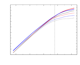
We encountered two difficulties in reproducing the three radial profiles in PA=31010𝑃superscript𝐴superscript310superscript10PA^{\prime}=310^{\circ}-10^{\circ}. First, the model intensity is lower than the observed intensity even at Σ0=1.26gcm2subscriptΣ01.26gsuperscriptcm2\Sigma_{0}=1.26\ \mathrm{g\ cm^{-2}}. In particular, it is 16%percent1616\% lower than I0,obssubscriptsuperscript𝐼0obsI^{*}_{0,\mathrm{obs}} in PA=330350𝑃superscript𝐴superscript330superscript350PA^{\prime}=330^{\circ}-350^{\circ}. Second, the model profiles in PA=310350𝑃superscript𝐴superscript310superscript350PA^{\prime}=310^{\circ}-350^{\circ} have larger radial extent than those observed even when the model width is set to be w0=21ausubscript𝑤021auw_{0}=21\ \mathrm{au}. The situation is shown more clearly in figure 5, where the model peak intensity I0subscriptsuperscript𝐼0I^{\prime}_{0} is plotted as a function of Σ0subscriptΣ0\Sigma_{0} for three sectors, PA=80100𝑃superscript𝐴superscript80superscript100PA^{\prime}=80^{\circ}-100^{\circ}, 35010superscript350superscript10350^{\circ}-10^{\circ}, and 260280superscript260superscript280260^{\circ}-280^{\circ}; they correspond to the far side, the major axis, and the near side, respectively. In Σ0<0.1gcm2subscriptΣ00.1gsuperscriptcm2\Sigma_{0}<0.1~{}\mathrm{g~{}cm^{-2}}, the peak intensities are roughly proportional to Σ0subscriptΣ0\Sigma_{0} and are the same for the far and near sides since the disk is optically thin. This can be confirmed in the model image shown in figure 3a. In Σ0>0.1gcm2subscriptΣ00.1gsuperscriptcm2\Sigma_{0}>0.1~{}\mathrm{g~{}cm^{-2}}, the slope is shallower for a higher Σ0subscriptΣ0\Sigma_{0}, and I0subscriptsuperscript𝐼0I^{\prime}_{0} reaches a ceiling. The ceiling of I0subscriptsuperscript𝐼0I^{\prime}_{0} is highest on the far side, followed by the major axis, and last, on the near side (figure 3b).

The saturation of the peak intensity can be understood as follows. At Σ00.1gcm2subscriptΣ00.1gsuperscriptcm2\Sigma_{0}\approx 0.1~{}\mathrm{g~{}cm^{-2}}, the effective optical thickness defined as

τeffΣ0κa(κa+κs)subscript𝜏effsubscriptΣ0subscript𝜅asubscript𝜅asubscript𝜅s\displaystyle\tau_{\mathrm{eff}}\approx\Sigma_{0}\sqrt{\kappa_{\mathrm{a}}(\kappa_{\mathrm{a}}+\kappa_{\mathrm{s}})} (12)

is approximately unity, while the optical thickness by absorption only is τa0.3subscript𝜏a0.3\tau_{\mathrm{a}}\approx 0.3. The effective optical thickness takes account of the diffusion length of a photon in the presence of scattering (Rybicki & Lightman (1979)). When τeffsubscript𝜏eff\tau_{\mathrm{eff}} is less than unity, the medium is effectively thin or translucent. Hence, the intensity is roughly proportional to the column density along the line of sight when the medium is isothermal (see Fig. 8 in Muto et al. (2015) for the temperature distribution). When Σ0>0.1gcm2subscriptΣ00.1gsuperscriptcm2\Sigma_{0}>0.1\ \mathrm{g\ cm^{-2}}, i.e., τeff>1subscript𝜏eff1\tau_{\mathrm{eff}}>1, the disk is opaque and the intensity reaches a ceiling. At the same time, the peak intensity depends on PA𝑃superscript𝐴PA^{\prime} for a given Σ0subscriptΣ0\Sigma_{0} model (figure 3b). The azimuthal dependence comes mainly from the difference in the temperature of the emitting surface, or the effective photosphere, which is discussed quantitatively in Section 5.2.

When Σ0>1.0gcm2subscriptΣ01.0gsuperscriptcm2\Sigma_{0}>1.0~{}\mathrm{g~{}cm^{-2}}, the intensity profile is also significantly broadened in the radial direction because the intensity becomes insensitive to the increase in Σ0subscriptΣ0\Sigma_{0}, i.e., the profile becomes saturated even before the beam convolution (figure 3). This situation can also be seen in table 2, where we have chosen the maximum Σ0subscriptΣ0\Sigma_{0} so that the peak intensity is as high as possible in our parameter space. The width in the model image, w0superscriptsubscript𝑤0w_{0}^{*}, is wider than the observed value, wobssubscriptsuperscript𝑤obsw^{*}_{\mathrm{obs}}, by more than 6%percent66\% in PA=310350𝑃superscript𝐴superscript310superscript350PA^{\prime}=310^{\circ}-350^{\circ}. Therefore, we conclude that the dust opacity applied here cannot reproduce the radial intensity profiles in PA=31010𝑃superscript𝐴superscript310superscript10PA^{\prime}=310^{\circ}-10^{\circ} due to the low intensity ceiling compared to the observation, as well as its associated effect of broadening the intensity profile.
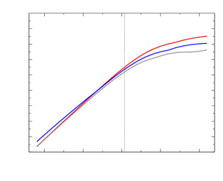
-1.2-1.0-0.8-0.6-0.4-0.20.00.20.40.6-2.0-1.5-1.0-0.50.0PA=80100𝑃superscript𝐴superscript80superscript100PA^{\prime}=80^{\circ}-100^{\circ}PA=35010𝑃superscript𝐴superscript350superscript10PA^{\prime}=350^{\circ}-10^{\circ}PA=260280𝑃superscript𝐴superscript260superscript280PA^{\prime}=260^{\circ}-280^{\circ}Refer to caption

log[I0/(1Jyasec2)]subscriptsuperscript𝐼01Jysuperscriptasec2\log\left[I^{\prime}_{\mathrm{0}}/\left(1\ \mathrm{Jy\ asec^{-2}}\right)\right]

log[Σ0/(1gcm2)]subscriptΣ01gsuperscriptcm2\log\left[\Sigma_{0}/\left(1\ \mathrm{g\ cm^{-2}}\right)\right]
Figure 5: The peak intensity I0subscriptsuperscript𝐼0I^{\prime}_{0} achievable in PA=80100𝑃superscript𝐴superscript80superscript100PA^{\prime}=80^{\circ}-100^{\circ} (the far side, red plots), PA=35010𝑃superscript𝐴superscript350superscript10PA^{\prime}=350^{\circ}-10^{\circ} (the major axis, blue plots), and PA=260280𝑃superscript𝐴superscript260superscript280PA^{\prime}=260^{\circ}-280^{\circ} (the near side, gray plots), regardless of rsuperscript𝑟r^{\prime}. The I0subscriptsuperscript𝐼0I^{\prime}_{0} values are values before beam convolution. In the analysis, w0subscript𝑤0w_{0} and r0subscript𝑟0r_{0} are fixed at 27au27au27\ \mathrm{au} and 175au175au175\ \mathrm{au}, respectively. The vertical, black dotted line denotes the Σ0subscriptΣ0\Sigma_{0} value where τeff=1subscript𝜏eff1\tau_{\mathrm{eff}}=1.

4.3 Uncertainties in the best fit values

Table 3: Fit values for PA=230250𝑃superscript𝐴superscript230superscript250PA^{*}=230^{\circ}-250^{\circ}.
Model parameters Model results
Σ0subscriptΣ0\Sigma_{0} w0subscript𝑤0w_{0} r0subscript𝑟0r_{0} Σ0w0subscriptΣ0subscript𝑤0\Sigma_{0}w_{0} Msecsubscript𝑀secM_{\mathrm{sec}} I0subscriptsuperscript𝐼0I^{*}_{0} w0subscriptsuperscript𝑤0w^{*}_{0} r0subscriptsuperscript𝑟0r^{*}_{0} ΔI0Δsubscriptsuperscript𝐼0\Delta I^{*}_{0} Δw0Δsubscriptsuperscript𝑤0\Delta w^{*}_{0} Δr0Δsubscriptsuperscript𝑟0\Delta r^{*}_{0}
(gcm2)gsuperscriptcm2\left(\mathrm{g\ cm^{-2}}\right) (au)au\left(\mathrm{au}\right) (au)au\left(\mathrm{au}\right) (gcm2au)gsuperscriptcm2au\left(\mathrm{g\ cm^{-2}\ au}\right) (M)subscript𝑀direct-product\left(M_{\odot}\right) (Jyasec2)Jysuperscriptasec2\left(\mathrm{Jy\ asec^{-2}}\right) (au)au\left(\mathrm{au}\right) (au)au\left(\mathrm{au}\right) (×I0,obs)\left(\times I^{\prime}_{0,\mathrm{obs}}\right) (au)au\left(\mathrm{au}\right) (au)au\left(\mathrm{au}\right)
8.31×1038.31superscript1038.31\times 10^{-3} 323232 195195195 0.270.270.27 3.0×1063.0superscript1063.0\times 10^{-6} 0.050.050.05 52.352.352.3 173.3173.3173.3 4.6×1054.6superscript1054.6\times 10^{-5} 0.70.7-0.7 0.80.80.8
8.85×1038.85superscript1038.85\times 10^{-3} 292929 195195195 0.260.260.26 2.9×1062.9superscript1062.9\times 10^{-6} 0.050.050.05 50.850.850.8 173.9173.9173.9 1.7×1051.7superscript1051.7\times 10^{-5} 0.80.80.8 0.30.30.3
Table 4: Fit values for PA=3050𝑃superscript𝐴superscript30superscript50PA^{\prime}=30^{\circ}-50^{\circ}.
Model parameters Model results
Σ0subscriptΣ0\Sigma_{0} w0subscript𝑤0w_{0} r0subscript𝑟0r_{0} Σ0w0subscriptΣ0subscript𝑤0\Sigma_{0}w_{0} Msecsubscript𝑀secM_{\mathrm{sec}} I0subscriptsuperscript𝐼0I^{*}_{0} w0subscriptsuperscript𝑤0w^{*}_{0} r0subscriptsuperscript𝑟0r^{*}_{0} ΔI0Δsubscriptsuperscript𝐼0\Delta I^{*}_{0} Δw0Δsubscriptsuperscript𝑤0\Delta w^{*}_{0} Δr0Δsubscriptsuperscript𝑟0\Delta r^{*}_{0}
(gcm2)gsuperscriptcm2\left(\mathrm{g\ cm^{-2}}\right) (au)au\left(\mathrm{au}\right) (au)au\left(\mathrm{au}\right) (gcm2au)gsuperscriptcm2au\left(\mathrm{g\ cm^{-2}\ au}\right) (M)subscript𝑀direct-product\left(M_{\odot}\right) (Jyasec2)Jysuperscriptasec2\left(\mathrm{Jy\ asec^{-2}}\right) (au)au\left(\mathrm{au}\right) (au)au\left(\mathrm{au}\right) (×I0,obs)\left(\times I^{\prime}_{0,\mathrm{obs}}\right) (au)au\left(\mathrm{au}\right) (au)au\left(\mathrm{au}\right)
1.121.121.12 212121 173173173 23.5223.5223.52 2.6×1052.6superscript1052.6\times 10^{-5} 1.251.251.25 50.750.750.7 152.6152.6152.6 2.9×1052.9superscript1052.9\times 10^{-5} 0.30.30.3 0.30.3-0.3
8.99×1018.99superscript1018.99\times 10^{-1} 232323 173173173 20.6820.6820.68 2.3×1052.3superscript1052.3\times 10^{-5} 1.251.251.25 51.751.751.7 152.1152.1152.1 1.8×1051.8superscript1051.8\times 10^{-5} 0.70.7-0.7 0.20.20.2

The best fit values cannot be strictly constrained because of the insufficient angular resolution (60auabsent60au\approx 60\ \mathrm{au} in FWHM). Furthermore, in the optically thick region the intensity reaches a ceiling, resulting in even larger uncertainties in the results, especially in Σ0subscriptΣ0\Sigma_{0}. The uncertainties in the optically thin and optically thick sectors are discussed separately, by using the radial profiles of PA=3050𝑃superscript𝐴superscript30superscript50PA^{\prime}=30^{\circ}-50^{\circ} and PA=230250𝑃superscript𝐴superscript230superscript250PA^{\prime}=230^{\circ}-250^{\circ} as case studies. We investigate the dependence of Msecsubscript𝑀secM_{\mathrm{sec}} on w0subscript𝑤0w_{0}, by treating Σ0subscriptΣ0\Sigma_{0} in equation (13) as the bound variable.

In the regime of optically thin and constant temperature,

I0Σ0w0,proportional-tosubscriptsuperscript𝐼0subscriptΣ0subscript𝑤0\displaystyle I^{*}_{0}\propto\Sigma_{0}w_{0}, (13)

i.e., the peak intensity is proportional to the product of Σ0subscriptΣ0\Sigma_{0} and w0subscript𝑤0w_{0}, or equivalently Msecsubscript𝑀secM_{\mathrm{sec}}. Despite the difference in their w0subscript𝑤0w_{0} values, the two parameter sets listed in table 4 for PA=230250𝑃superscript𝐴superscript230superscript250PA^{\prime}=230^{\circ}-250^{\circ} satisfy the criteria in equation (3.4). The two sets, each with w0=32ausubscript𝑤032auw_{0}=32\ \mathrm{au} and w0=29ausubscript𝑤029auw_{0}=29\ \mathrm{au}, estimate Msecsubscript𝑀secM_{\mathrm{sec}} to be 3.0×10⁶M3.0superscript106subscript𝑀direct-product3.0\times 10^{-6}\ M_{\odot} and 2.9×10⁶M2.9superscript106subscript𝑀direct-product2.9\times 10^{-6}\ M_{\odot}, respectively. Both Σ0subscriptΣ0\Sigma_{0} and w0subscript𝑤0w_{0} contain ±10%plus-or-minuspercent10\pm 10\% uncertainties due to the criteria tolerance in equation (3.4), but Msecsubscript𝑀secM_{\mathrm{sec}} is uncertain only by approximately ±5%plus-or-minuspercent5\pm 5\%. This is because I0subscriptsuperscript𝐼0I^{*}_{0} is proportional to Msecsubscript𝑀secM_{\mathrm{sec}} in these optically thin sectors.

Similarly, in table 4 we listed two parameter sets for the optically thick PA=3050𝑃superscript𝐴superscript30superscript50PA^{\prime}=30^{\circ}-50^{\circ}. The difference in terms of Msecsubscript𝑀secM_{\mathrm{sec}} or Σ0w0subscriptΣ0subscript𝑤0\Sigma_{0}w_{0} is about 11%percent1111\%, which is much larger than that for PA=230250𝑃superscript𝐴superscript230superscript250PA^{\prime}=230^{\circ}-250^{\circ}. The difference in terms of w0subscript𝑤0w_{0} is about 10%percent1010\%, in contrast to the difference in Σ0subscriptΣ0\Sigma_{0} which reaches 20%percent2020\%. This implies that equation (13) breaks down when the intensity reaches a ceiling. Moreover, if we relax the criteria tolerance to follow Muto et al. (2015) (Section 3.4), a wider range of Σ0w0subscriptΣ0subscript𝑤0\Sigma_{0}w_{0} can be obtained as best fit values, so as the uncertainties in the optically thick sectors (refer to Appendix 2 in Muto et al. 2015). This explains the discrepancy between our results and those derived by Muto et al. (2015): in this work the Σ0subscriptΣ0\Sigma_{0} value for PA=3050𝑃superscript𝐴superscript30superscript50PA^{\prime}=30^{\circ}-50^{\circ} is about twice the value derived by Muto et al. (2015), resulting in the higher Σ0subscriptΣ0\Sigma_{0} contrast between PA=3050𝑃superscript𝐴superscript30superscript50PA^{\prime}=30^{\circ}-50^{\circ} and PA=230250𝑃superscript𝐴superscript230superscript250PA^{\prime}=230^{\circ}-250^{\circ}. The best fit results, especially the values of Σ0subscriptΣ0\Sigma_{0} in the optically thick region in PA=10130𝑃superscript𝐴superscript10superscript130PA^{\prime}=10^{\circ}-130^{\circ} and PA=290310𝑃superscript𝐴superscript290superscript310PA^{\prime}=290^{\circ}-310^{\circ}, contain uncertainties of a factor of 2similar-toabsent2\sim 2. Analysis based on observations with a higher angular resolution, or at a longer wavelength (thus less opaque in the emissions), should be able to better constrain Σ0subscriptΣ0\Sigma_{0} and w0subscript𝑤0w_{0}.

5 Discussions

Table 5: Derived best fit values using the reduced-scattering model.
PA𝑃superscript𝐴PA^{\prime} Σ0subscriptΣ0\Sigma_{0} w0subscript𝑤0w_{0} r0subscript𝑟0r_{0} Msecsubscript𝑀secM_{\mathrm{sec}} ΔI0Δsubscriptsuperscript𝐼0\Delta I^{*}_{0} Δw0Δsubscriptsuperscript𝑤0\Delta w^{*}_{0} Δr0Δsubscriptsuperscript𝑟0\Delta r^{*}_{0}
(gcm2)gsuperscriptcm2(\mathrm{g\ cm^{-2}}) (au)au(\mathrm{au}) (au)au(\mathrm{au}) (M)subscript𝑀direct-product(M_{\odot}) (×I0,obs)\left(\times I^{*}_{0,\mathrm{obs}}\right) (au)au\left(\mathrm{au}\right) (au)au\left(\mathrm{au}\right)
1030superscript10superscript3010^{\circ}-30^{\circ} 2.76×1012.76superscript1012.76\times 10^{-1} 313131 173173173 1.0×1041.0superscript1041.0\times 10^{-4} 4.0×1054.0superscript105-4.0\times 10^{-5} +0.90.9+0.9 0.00.0-0.0
3050superscript30superscript5030^{\circ}-50^{\circ} 3.34×1013.34superscript1013.34\times 10^{-1} 313131 173173173 1.1×1041.1superscript1041.1\times 10^{-4} 2.6×1052.6superscript105-2.6\times 10^{-5} 0.60.6-0.6 0.90.9-0.9
5070superscript50superscript7050^{\circ}-70^{\circ} 3.33×1013.33superscript1013.33\times 10^{-1} 292929 173173173 9.8×1059.8superscript1059.8\times 10^{-5} 2.7×1052.7superscript105-2.7\times 10^{-5} 0.80.8-0.8 0.50.5-0.5
7090superscript70superscript9070^{\circ}-90^{\circ} 2.46×1012.46superscript1012.46\times 10^{-1} 272727 169169169 6.1×1056.1superscript1056.1\times 10^{-5} 2.2×1052.2superscript105-2.2\times 10^{-5} 0.50.5-0.5 0.60.6-0.6
90110superscript90superscript110\phantom{1}90^{\circ}-110^{\circ} 1.84×1011.84superscript1011.84\times 10^{-1} 232323 167167167 3.9×1053.9superscript1053.9\times 10^{-5} 3.1×1053.1superscript105-3.1\times 10^{-5} +0.00.0+0.0 0.90.9-0.9
110130superscript110superscript130110^{\circ}-130^{\circ} 1.24×1011.24superscript1011.24\times 10^{-1} 232323 165165165 2.8×1052.8superscript1052.8\times 10^{-5} 2.8×1052.8superscript105-2.8\times 10^{-5} +0.10.1+0.1 +0.20.2+0.2
130150superscript130superscript150130^{\circ}-150^{\circ} 6.94×1026.94superscript1026.94\times 10^{-2} 272727 167167167 2.0×1052.0superscript1052.0\times 10^{-5} 2.7×1052.7superscript105-2.7\times 10^{-5} 0.70.7-0.7 0.70.7-0.7
150170superscript150superscript170150^{\circ}-170^{\circ} 3.32×1023.32superscript1023.32\times 10^{-2} 292929 171171171 1.1×1051.1superscript1051.1\times 10^{-5} 1.9×1051.9superscript105-1.9\times 10^{-5} 0.20.2-0.2 0.90.9-0.9
170190superscript170superscript190170^{\circ}-190^{\circ} 1.51×1021.51superscript1021.51\times 10^{-2} 313131 177177177 5.7×1065.7superscript1065.7\times 10^{-6} 1.0×1051.0superscript105-1.0\times 10^{-5} 0.40.4-0.4 0.50.5-0.5
190210superscript190superscript210190^{\circ}-210^{\circ} 1.07×1021.07superscript1021.07\times 10^{-2} 292929 187187187 3.9×1063.9superscript1063.9\times 10^{-6} 9.1×1069.1superscript106-9.1\times 10^{-6} +0.70.7+0.7 +0.60.6+0.6
210230superscript210superscript230210^{\circ}-230^{\circ} 8.97×1038.97superscript1038.97\times 10^{-3} 323232 193193193 3.5×1063.5superscript1063.5\times 10^{-6} 3.5×1053.5superscript105-3.5\times 10^{-5} 0.50.5-0.5 0.20.2-0.2
230250superscript230superscript250230^{\circ}-250^{\circ} 8.28×1038.28superscript1038.28\times 10^{-3} 323232 195195195 3.0×1063.0superscript1063.0\times 10^{-6} 1.5×1051.5superscript105-1.5\times 10^{-5} 0.60.6-0.6 +0.10.1+0.1
250270superscript250superscript270250^{\circ}-270^{\circ} 2.80×1022.80superscript1022.80\times 10^{-2} 232323 185185185 6.5×1066.5superscript1066.5\times 10^{-6} 4.4×1054.4superscript105-4.4\times 10^{-5} +0.10.1+0.1 0.30.3-0.3
270290superscript270superscript290270^{\circ}-290^{\circ} 7.26×1027.26superscript1027.26\times 10^{-2} 272727 183183183 2.0×1052.0superscript1052.0\times 10^{-5} 7.5×1077.5superscript107-7.5\times 10^{-7} 0.30.3-0.3 +0.90.9+0.9
290310superscript290superscript310290^{\circ}-310^{\circ} 1.46×1011.46superscript1011.46\times 10^{-1} 272727 181181181 4.2×1054.2superscript1054.2\times 10^{-5} 8.1×1078.1superscript107-8.1\times 10^{-7} 0.10.1-0.1 0.60.6-0.6
310330superscript310superscript330310^{\circ}-330^{\circ} 2.37×1012.37superscript1012.37\times 10^{-1} 292929 177177177 7.7×1057.7superscript1057.7\times 10^{-5} 1.1×1051.1superscript105-1.1\times 10^{-5} +0.00.0+0.0 +0.30.3+0.3
330350superscript330superscript350330^{\circ}-350^{\circ} 2.91×1012.91superscript1012.91\times 10^{-1} 292929 175175175 1.0×1041.0superscript1041.0\times 10^{-4} 2.2×1052.2superscript105-2.2\times 10^{-5} +0.70.7+0.7 0.40.4-0.4
35010superscript350superscript10350^{\circ}-10^{\circ}\phantom{3} 2.59×1012.59superscript1012.59\times 10^{-1} 313131 173173173 9.6×1059.6superscript1059.6\times 10^{-5} 2.2×1052.2superscript105-2.2\times 10^{-5} +0.60.6+0.6 0.90.9-0.9
-0.200.000.200.400.600.801.001.201.40050100150200250300350Σ0=3.34×101gcm2subscriptΣ03.34superscript101gsuperscriptcm2\Sigma_{0}=3.34\times 10^{-1}\ \mathrm{g\ cm^{-2}}w0=31ausubscript𝑤031auw_{0}=31\ \mathrm{au}r0=173ausubscript𝑟0173aur_{0}=173\ \mathrm{au}Msec=1.1×10⁴Msubscript𝑀sec1.1superscript104subscript𝑀direct-productM_{\mathrm{sec}}=1.1\times 10^{-4}\ M_{\odot}Refer to caption

I(Jyasec2)superscript𝐼Jysuperscriptasec2I^{*}\left(\mathrm{Jy\ asec^{-2}}\right)

r(au)superscript𝑟aur^{*}\left(\mathrm{au}\right)PA=3050𝑃superscript𝐴superscript30superscript50PA^{\prime}=30^{\circ}-50^{\circ}
(a)
-0.020.000.020.040.060.080.100.12050100150200250300350Σ0=1.51×10²gcm2subscriptΣ01.51superscript102gsuperscriptcm2\Sigma_{0}=1.51\times 10^{-2}\ \mathrm{g\ cm^{-2}}w0=31ausubscript𝑤031auw_{0}=31\ \mathrm{au}r0=177ausubscript𝑟0177aur_{0}=177\ \mathrm{au}Msec=5.6×10⁶Msubscript𝑀sec5.6superscript106subscript𝑀direct-productM_{\mathrm{sec}}=5.6\times 10^{-6}\ M_{\odot}Refer to caption

I(Jyasec2)superscript𝐼Jysuperscriptasec2I^{*}\left(\mathrm{Jy\ asec^{-2}}\right)

r(au)superscript𝑟aur^{*}\left(\mathrm{au}\right)PA=170190𝑃superscript𝐴superscript170superscript190PA^{\prime}=170^{\circ}-190^{\circ}
(b)
-0.010.000.010.020.030.040.050.06050100150200250300350Σ0=8.28×10³gcm2subscriptΣ08.28superscript103gsuperscriptcm2\Sigma_{0}=8.28\times 10^{-3}\ \mathrm{g\ cm^{-2}}w0=32ausubscript𝑤032auw_{0}=32\ \mathrm{au}r0=195ausubscript𝑟0195aur_{0}=195\ \mathrm{au}Msec=3.0×10⁶Msubscript𝑀sec3.0superscript106subscript𝑀direct-productM_{\mathrm{sec}}=3.0\times 10^{-6}\ M_{\odot}Refer to caption

I(Jyasec2)superscript𝐼Jysuperscriptasec2I^{*}\left(\mathrm{Jy\ asec^{-2}}\right)

r(au)superscript𝑟aur^{*}\left(\mathrm{au}\right)PA=230250𝑃superscript𝐴superscript230superscript250PA^{\prime}=230^{\circ}-250^{\circ}
(c)
0.000.100.200.300.400.500.600.700.800.901.00050100150200250300350Σ0=2.37×101gcm2subscriptΣ02.37superscript101gsuperscriptcm2\Sigma_{0}=2.37\times 10^{-1}\ \mathrm{g\ cm^{-2}}w0=29ausubscript𝑤029auw_{0}=29\ \mathrm{au}r0=177ausubscript𝑟0177aur_{0}=177\ \mathrm{au}Msec=7.7×10⁵Msubscript𝑀sec7.7superscript105subscript𝑀direct-productM_{\mathrm{sec}}=7.7\times 10^{-5}\ M_{\odot}Refer to caption

I(Jyasec2)superscript𝐼Jysuperscriptasec2I^{*}\left(\mathrm{Jy\ asec^{-2}}\right)

r(au)superscript𝑟aur^{*}\left(\mathrm{au}\right)PA=310330𝑃superscript𝐴superscript310superscript330PA^{\prime}=310^{\circ}-330^{\circ}
(d)
-0.200.000.200.400.600.801.001.20050100150200250300350Σ0=2.91×101gcm2subscriptΣ02.91superscript101gsuperscriptcm2\Sigma_{0}=2.91\times 10^{-1}\ \mathrm{g\ cm^{-2}}w0=29ausubscript𝑤029auw_{0}=29\ \mathrm{au}r0=175ausubscript𝑟0175aur_{0}=175\ \mathrm{au}Msec=1.0×10⁴Msubscript𝑀sec1.0superscript104subscript𝑀direct-productM_{\mathrm{sec}}=1.0\times 10^{-4}\ M_{\odot}Refer to caption

I(Jyasec2)superscript𝐼Jysuperscriptasec2I^{*}\left(\mathrm{Jy\ asec^{-2}}\right)

r(au)superscript𝑟aur^{*}\left(\mathrm{au}\right)PA=330350𝑃superscript𝐴superscript330superscript350PA^{\prime}=330^{\circ}-350^{\circ}
(e)
0.000.200.400.600.801.001.20050100150200250300350Σ0=2.59×101gcm2subscriptΣ02.59superscript101gsuperscriptcm2\Sigma_{0}=2.59\times 10^{-1}\ \mathrm{g\ cm^{-2}}w0=31ausubscript𝑤031auw_{0}=31\ \mathrm{au}r0=173ausubscript𝑟0173aur_{0}=173\ \mathrm{au}Msec=9.3×10⁵Msubscript𝑀sec9.3superscript105subscript𝑀direct-productM_{\mathrm{sec}}=9.3\times 10^{-5}\ M_{\odot}Refer to caption

I(Jyasec2)superscript𝐼Jysuperscriptasec2I^{*}\left(\mathrm{Jy\ asec^{-2}}\right)

r(au)superscript𝑟aur^{*}\left(\mathrm{au}\right)PA=35010𝑃superscript𝐴superscript350superscript10PA^{\prime}=350^{\circ}-10^{\circ}
(f)
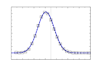
Figure 6: Similar to figure 4, but the results (blue solid lines) here are derived by the reduced-scattering model. The radial profiles of PA=310330𝑃superscript𝐴superscript310superscript330PA^{\prime}=310^{\circ}-330^{\circ}, PA=330350𝑃superscript𝐴superscript330superscript350PA^{\prime}=330^{\circ}-350^{\circ}, and PA=35010𝑃superscript𝐴superscript350superscript10PA^{\prime}=350^{\circ}-10^{\circ} are well reproduced with the reduced-scattering model.
-1.2-1.0-0.8-0.6-0.4-0.20.00.20.40.6-2.0-1.5-1.0-0.50.0Conventional Model: dashed linesScattering-Reduced Model: solid linesPA=80100𝑃superscript𝐴superscript80superscript100PA^{\prime}=80^{\circ}-100^{\circ}PA=35010𝑃superscript𝐴superscript350superscript10PA^{\prime}=350^{\circ}-10^{\circ}PA=260280𝑃superscript𝐴superscript260superscript280PA^{\prime}=260^{\circ}-280^{\circ}Refer to caption

log[I0/(1Jyasec2)]subscriptsuperscript𝐼01Jysuperscriptasec2\log\left[I^{\prime}_{\mathrm{0}}/\left(1\ \mathrm{Jy\ asec^{-2}}\right)\right]

log[Σ0/(1gcm2)]subscriptΣ01gsuperscriptcm2\log\left[\Sigma_{0}/\left(1\ \mathrm{g\ cm^{-2}}\right)\right]
Figure 7: The maximum surface brightness I0subscriptsuperscript𝐼0I^{\prime}_{0} achievable in PA=80100𝑃superscript𝐴superscript80superscript100PA^{\prime}=80^{\circ}-100^{\circ} (red plots), PA=35010𝑃superscript𝐴superscript350superscript10PA^{\prime}=350^{\circ}-10^{\circ} (blue plots), and PA=260280𝑃superscript𝐴superscript260superscript280PA^{\prime}=260^{\circ}-280^{\circ} (gray plots), regardless of rsuperscript𝑟r^{\prime}. Solid and dashed lines are the results using the reduced-scattering and conventional models, respectively. The I0subscriptsuperscript𝐼0I^{\prime}_{0} values are values before beam convolution. The vertical, black dotted line denotes the Σ0subscriptΣ0\Sigma_{0} value where τeff=1subscript𝜏eff1\tau_{\mathrm{eff}}=1 in the reduced-scattering model.

5.1 Reducing scattering opacities
-2.5-2.0-1.5-1.0-0.50.00.520253035160170180190200-6.0-5.5-5.0-4.5-4.0-3.5-3.004080120160200240280320Refer to caption

log[Σ0/(1gcm2)]subscriptΣ01gsuperscriptcm2\log\left[\Sigma_{0}\ /\left(1\ \mathrm{g\ cm^{-2}}\right)\right]

-2.5-2.0-1.5-1.0-0.50.00.5

w0(au)subscript𝑤0auw_{0}\ \left(\mathrm{au}\right)

20253035

r0(au)subscript𝑟0aur_{0}\ \left(\mathrm{au}\right)

160170180190200

log[Msec/(1M)]subscript𝑀sec1subscript𝑀direct-product\log\left[M_{\mathrm{sec}}/\left(1\ M_{\odot}\right)\right]

PA()PA^{\prime}\ \left({}^{\circ}\right)-6.0-5.5-5.0-4.5-4.0-3.5-3.004080120160200240280320
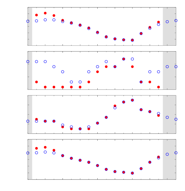
Figure 8: The best fit parameters, Σ0subscriptΣ0\Sigma_{0}, w0subscript𝑤0w_{0}, r0subscript𝑟0r_{0}, and Msecsubscript𝑀secM_{\mathrm{sec}}, distributions along the PA𝑃superscript𝐴PA^{\prime} direction, derived using the conventional (red filled circles) and the reduced-scattering model (blue open circles). The gray shaded portions indicate the PA𝑃superscript𝐴PA^{\prime} sectors where the radial profiles cannot be reproduced by the conventional model.

Figure 5 shows that I0subscriptsuperscript𝐼0I^{\prime}_{0} depends on both Σ0subscriptΣ0\Sigma_{0} and PA𝑃superscript𝐴PA^{\prime}, and it reaches a ceiling when τeffsubscript𝜏eff\tau_{\mathrm{eff}} exceeds unity. The low intensity ceiling is a consequence of the large scattering optical depth. Although the conventional properties of the dust grains are applied in the model, their actual opacity can be highly uncertain; they might be aggregates composed of monomers and have different composition (Tazaki et al., 2016), so that either the scattering cross section might have been overestimated or the asymmetry parameter been underestimated, or both. Therefore, as a tentative approach to reproduce the radial profiles in the northwestern region, PA=31010𝑃superscript𝐴superscript310superscript10PA^{\prime}=310^{\circ}-10^{\circ}, we reduce the scattering opacity across all the wavelengths by 90%percent9090\%, as depicted in figure 2. The scattering opacity at λobssubscript𝜆obs\lambda_{\mathrm{obs}} is then reduced to 2.62cm2g12.62superscriptcm2superscriptg12.62\ \mathrm{cm^{2}\ g^{-1}}, which approximates the absorption opacity. The purpose is to reduce the scattering optical depth, thus elevating the ceiling of I0subscriptsuperscript𝐼0I^{\prime}_{0}. The absorption opacity of the dust particles is kept the same. Therefore the albedo η𝜂\eta is thus effectively reduced. In the following, we denote this model by “reduced-scattering model”, in contrast to the “conventional model” which uses the conventional scattering opacity. We apply the reduced-scattering model to reproduce not only the radial profiles of the northwestern region, but also to all PA𝑃superscript𝐴PA^{\prime} sectors in order to study the relevant effects.

The results are shown in figure 6 and in table 5. We successfully reproduce the radial profiles in all sectors, including those in PA=31010𝑃superscript𝐴superscript310superscript10PA^{\prime}=310^{\circ}-10^{\circ} (figure 6d, 6e, and 6f). In addition, the contrast in Σ0subscriptΣ0\Sigma_{0} between PA=3050𝑃superscript𝐴superscript30superscript50PA^{\prime}=30^{\circ}-50^{\circ} and PA=230250𝑃superscript𝐴superscript230superscript250PA^{\prime}=230^{\circ}-250^{\circ} is reduced to about a factor of 404040, which is closer to the contrast in observed intensity. Using the reduced-scattering model, we plot I0subscriptsuperscript𝐼0I^{\prime}_{0} as a function of Σ0subscriptΣ0\Sigma_{0} in figure 7. The results are essentially similar to those of the conventional model, but I0subscriptsuperscript𝐼0I^{\prime}_{0} reaches a ceiling only at Σ00.25gcm2subscriptΣ00.25gsuperscriptcm2\Sigma_{0}\approx 0.25\ \mathrm{g\ cm^{-2}}, at which τeff1subscript𝜏eff1\tau_{\mathrm{eff}}\approx 1. Besides, the reduced-scattering model is brighter than the conventional model in all the cases, especially when Σ0subscriptΣ0\Sigma_{0} exceeds 0.1gcm20.1gsuperscriptcm20.1\ \mathrm{g\ cm^{-2}}, where τeffsubscript𝜏eff\tau_{\mathrm{eff}} is approximately 111 in the conventional model but only 0.30.30.3 in the reduced-scattering model.

We summarize the best fit parameters and the dust masses derived from the conventional and the reduced-scattering models in figure 8. Compared to the conventional model, the reduced-scattering model estimates smaller Σ0subscriptΣ0\Sigma_{0} but larger w0subscript𝑤0w_{0} in the northern region. Furthermore, the Σ0subscriptΣ0\Sigma_{0} distribution in PA=31070𝑃superscript𝐴superscript310superscript70PA^{\prime}=310^{\circ}-70^{\circ} is about 0.3gcm20.3gsuperscriptcm20.3\ \mathrm{g\ cm^{-2}} on average, contrary to the conventional model which derives about 0.9gcm20.9gsuperscriptcm20.9\ \mathrm{g\ cm^{-2}} for sectors in PA=1070𝑃superscript𝐴superscript10superscript70PA^{\prime}=10^{\circ}-70^{\circ}. When scattering is dominant, the disk appearance is faint and indistinct, restricting only the model of small w0subscript𝑤0w_{0} and large Σ0subscriptΣ0\Sigma_{0} to reproduce w0,obssubscriptsuperscript𝑤0obsw^{*}_{0,\mathrm{obs}}. Reducing the scattering opacities sharpens the disk outline and thus allows us to reproduce the same I0subscriptsuperscript𝐼0I^{*}_{0} with a larger w0subscript𝑤0w_{0} but at a smaller Σ0subscriptΣ0\Sigma_{0}, as predicted by equation (13). Since the reduced-scattering model is yet to be optically thick for the intensity to reach a ceiling, it estimates about half the mass derived from the conventional model. The sectors within PA=130290𝑃superscript𝐴superscript130superscript290PA^{\prime}=130^{\circ}-290^{\circ} show no significant changes in their best fit parameters like those in the northern region; their τeffsubscript𝜏eff\tau_{\mathrm{eff}} values are below unity so that the intensity is not much different between the conventional and reduced-scattering models. As a conclusion, reducing scattering opacity alters the results only in the optically thick northern sectors.

5.2 Intensity Dependence on Scattering Opacity and PA𝑃superscript𝐴PA^{\prime}
Refer to caption100120140160180200220240r(au)𝑟aur\ \left(\mathrm{au}\right)-60-40-200204060

z(au)𝑧auz\ \left(\mathrm{au}\right)

01.0×10141.0superscript10141.0\times 10^{-14}2.0×10142.0superscript10142.0\times 10^{-14}3.0×10143.0superscript10143.0\times 10^{-14}(κa+κs)ρSνeτ(Jyasec2au1)subscript𝜅asubscript𝜅s𝜌subscript𝑆𝜈superscriptesuperscript𝜏Jysuperscriptasec2superscriptau1(\kappa_{\mathrm{a}}+\kappa_{\mathrm{s}})\rho S_{\nu}\mathrm{e}^{-\tau^{\prime}}\ \left(\mathrm{Jy\ asec^{-2}\ au^{-1}}\right)707070606060505050404040303030202020
(a) θ=27𝜃superscript27\theta=-27^{\circ}
Refer to caption100120140160180200220240r(au)𝑟aur\ \left(\mathrm{au}\right)-60-40-200204060

z(au)𝑧auz\ \left(\mathrm{au}\right)

01.0×10141.0superscript10141.0\times 10^{-14}2.0×10142.0superscript10142.0\times 10^{-14}3.0×10143.0superscript10143.0\times 10^{-14}(κa+κs)ρSνeτ(Jyasec2au1)subscript𝜅asubscript𝜅s𝜌subscript𝑆𝜈superscriptesuperscript𝜏Jysuperscriptasec2superscriptau1(\kappa_{\mathrm{a}}+\kappa_{\mathrm{s}})\rho S_{\nu}\mathrm{e}^{-\tau^{\prime}}\ \left(\mathrm{Jy\ asec^{-2}\ au^{-1}}\right)707070606060505050404040303030202020
(b) θ=0𝜃superscript0\theta=0^{\circ}
Refer to caption100120140160180200220240r(au)𝑟aur\ \left(\mathrm{au}\right)-60-40-200204060

z(au)𝑧auz\ \left(\mathrm{au}\right)

01.0×10141.0superscript10141.0\times 10^{-14}2.0×10142.0superscript10142.0\times 10^{-14}3.0×10143.0superscript10143.0\times 10^{-14}(κa+κs)ρSνeτ(Jyasec2au1)subscript𝜅asubscript𝜅s𝜌subscript𝑆𝜈superscriptesuperscript𝜏Jysuperscriptasec2superscriptau1(\kappa_{\mathrm{a}}+\kappa_{\mathrm{s}})\rho S_{\nu}\mathrm{e}^{-\tau^{\prime}}\ \left(\mathrm{Jy\ asec^{-2}\ au^{-1}}\right)707070606060505050404040303030202020
(c) θ=+27𝜃superscript27\theta=+27^{\circ}
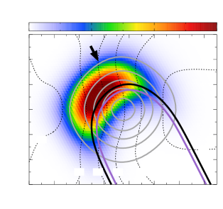
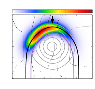
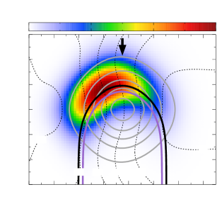
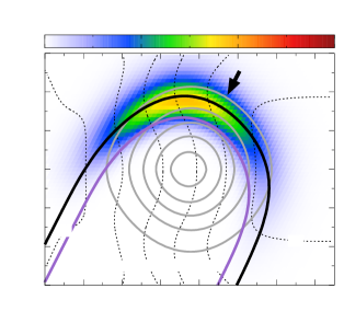
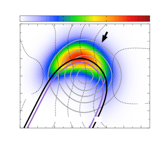
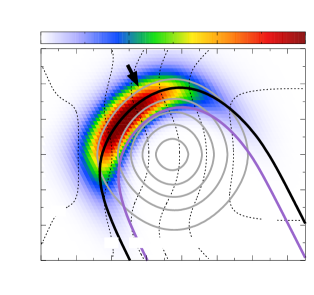
Figure 9: The (κa+κs)ρSνexp(τ)subscript𝜅asubscript𝜅s𝜌subscript𝑆𝜈superscript𝜏(\kappa_{\mathrm{a}}+\kappa_{\mathrm{s}})\rho S_{\nu}\exp(-\tau^{\prime}) distributions of the conventional (left panels) and the reduced-scattering model (right panels), at a common Σ0=1.00gcm2subscriptΣ01.00gsuperscriptcm2\Sigma_{0}=1.00\ \mathrm{g\ cm^{-2}}. The color scale is common for each panel. The top, middle, and bottom panels are the distributions at viewing angle θ=27𝜃superscript27\theta=-27^{\circ}, 0superscript00^{\circ}, and +27superscript27+27^{\circ}, respectively, as indicated by the black arrows. The black dotted contours are the temperature (units in KK\mathrm{K}). The gray solid contours are the densities drawn at ρ(r,z)=0.1, 0.3, 0.5, 0.7, 0.9𝜌𝑟𝑧0.10.30.50.70.9\rho(r,z)=0.1\ ,\ 0.3\ ,\ 0.5\ ,\ 0.7,\ 0.9 of ρ0(175au,0au)=1.3×10¹⁵gcm3subscript𝜌0175au0au1.3superscript1015gsuperscriptcm3\rho_{0}(175\ \mathrm{au},0\ \mathrm{au})=1.3\times 10^{-15}\ \mathrm{g\ cm^{-3}}, the peak density in the model. The surface where τ=1superscript𝜏1\tau^{\prime}=1 and τeff=1subscript𝜏eff1\tau_{\mathrm{eff}}=1 are indicated by the thick black and the purple curves, respectively.

In this subsection we discuss why the reduced-scattering model can reproduce the ALMA observation while the conventional model cannot. We also discuss the origin of the azimuthal dependence of the peak intensity. For these purposes, we evaluate the model intensity quantitatively.

The solution of equation (8) is expressed as

I(r;PA)=(κa+κs)+ρ(r,z)Sν(r,z)eτ𝑑z,superscript𝐼𝑟𝑃superscript𝐴subscript𝜅asubscript𝜅ssubscriptsuperscript𝜌𝑟𝑧subscript𝑆𝜈𝑟𝑧superscript𝑒superscript𝜏differential-dsuperscript𝑧\displaystyle I^{\prime}(r;PA^{\prime})=(\kappa_{\mathrm{a}}+\kappa_{\mathrm{s}})\int^{+\infty}_{-\infty}\rho(r,z)S_{\nu}(r,z)e^{-\tau^{\prime}}dz^{\prime}, (14)

where τsuperscript𝜏\tau^{\prime} denotes the optical depth measured from the observer to the point (r,z)𝑟𝑧(r,z) in the disk along the line of sight zsuperscript𝑧z^{\prime}, defined by

τ(r,z;PA)=(κa+κs)+zρ𝑑z.superscript𝜏𝑟𝑧𝑃superscript𝐴subscript𝜅asubscript𝜅ssubscriptsuperscript𝑧𝜌differential-dsuperscript𝑧\displaystyle\tau^{\prime}(r,z;PA^{\prime})=(\kappa_{\mathrm{a}}+\kappa_{\mathrm{s}})\int^{z}_{{+\infty}}\rho dz^{\prime}. (15)

The observer is located at z=+𝑧z=+\infty. The observable photon density, (κa+κs)ρSνexp(τ)subscript𝜅asubscript𝜅s𝜌subscript𝑆𝜈superscript𝜏(\kappa_{\mathrm{a}}+\kappa_{\mathrm{s}})\rho S_{\nu}\exp(-\tau^{\prime}), denotes the emissivity per unit length in which absorption and scattering are taken into account by the attenuation factor exp(τ)superscript𝜏\exp(-\tau^{\prime}). Figure 9 shows the observable photon density in unit of Jyasec2au1Jysuperscriptasec2superscriptau1\mathrm{Jy\ asec^{-2}\ au^{-1}} for the model of Σ0=1.00gcm2subscriptΣ01.00gsuperscriptcm2\Sigma_{0}=1.00\ \mathrm{g\ cm^{-2}}, w0=27ausubscript𝑤027auw_{0}=27\ \mathrm{au}, and r0=175ausubscript𝑟0175aur_{0}=175\ \mathrm{au}. The left and right panels are based on the conventional and the reduced-scattering models, respectively. From top to bottom, the line of sight is offset from the z𝑧z-axis by θ=27𝜃superscript27\theta=-27^{\circ}, 0superscript00^{\circ}, and +27superscript27+27^{\circ}. Since the inclination of the disk is i=27𝑖superscript27i=27^{\circ}, the top panels correspond to PA=90𝑃superscript𝐴superscript90PA^{\prime}=90^{\circ} (the far side) while the bottom panels to PA=270𝑃superscript𝐴superscript270PA^{\prime}=270^{\circ} (the near side). The middle panels where θ=0𝜃superscript0\theta=0^{\circ} shows the observable photon density of a face-on disk; they do not actually correspond to PA=0𝑃superscript𝐴superscript0PA^{\prime}=0^{\circ} because our line of sight does not lie in the (r,z)𝑟𝑧(r,z) plane. However, the results can be regarded as a good substitute for the PA=0𝑃superscript𝐴superscript0PA^{\prime}=0^{\circ} case since the inclination angle is small.

In each panel of figure 9, the gray solid and black dotted contours denote the density and temperature, respectively. The density and temperature are almost unchanged by the reduction of scattering. The observable photon density, on the other hand, is greatly different between the conventional and the scattering-reduced models, and it also varies with θ𝜃\theta. The thick black and purple curves denote the location of τ=1superscript𝜏1\tau^{\prime}=1 and τeff=1subscript𝜏eff1\tau_{\mathrm{eff}}=1, respectively; the location of τeff=1subscript𝜏eff1\tau_{\mathrm{eff}}=1 is plotted by scaling τsuperscript𝜏\tau^{\prime} by a factor of (1η)1/2superscript1𝜂12(1-\eta)^{-1/2}.

The observed photons come mainly from the region of τ=1superscript𝜏1\tau^{\prime}=1, where τeffsubscript𝜏eff\tau_{\mathrm{eff}} is still smaller than unity. This is because while most of the photons are often emitted from the τeff=1subscript𝜏eff1\tau_{\mathrm{eff}}=1 surface, the observed photons are scattered around τ=1superscript𝜏1\tau^{\prime}=1 surface before reaching the observer. In the conventional model, the difference between τeff=1subscript𝜏eff1\tau_{\mathrm{eff}}=1 and τ=1superscript𝜏1\tau^{\prime}=1 is large, and its observable photon emitting area is confined in a narrow region near τ=1superscript𝜏1\tau^{\prime}=1 (left panels in figure 9). When the reduced-scattering model is applied, the regions of τeff=1subscript𝜏eff1\tau_{\mathrm{eff}}=1 and τ=1superscript𝜏1\tau^{\prime}=1 become closer and the observable photon density extends over a wider area (right panels in figure 9). The narrowing of the emitting area in the conventional model is equivalent to the decrease in propagation speed of the photons caused by the dominant scattering. Considering that the source function of radiation is similar in both models, the intensity is higher in the reduced-scattering model because the line of sight crosses a longer path in the area of high observable photon density. It should be noted that the model peak intensity is lower than that of the blackbody radiation for the dust temperature in the presence of scattering.

The effects of scattering on the intensity is serious only when κs>κasubscript𝜅ssubscript𝜅a\kappa_{\mathrm{s}}>\kappa_{\mathrm{a}}. Further reduction in the scattering opacity will increase the intensity only by a little, thus we cannot set a lower limit on the scattering opacity from our modeling. Nevertheless, the scattering opacity of the dust grains should be appreciable since the pattern of polarization in the disk at λ=890μm𝜆890𝜇m\lambda=890\ \mu\mathrm{m}, recently revealed by ALMA, seems consistent with the case of self-scattering (Kataoka et al., 2015, 2016).

The peak intensity shows azimuthal dependence when the disk is inclined, and the observed intensity strongly depends on the temperature of the effective photosphere when τsuperscript𝜏\tau^{\prime} (or τeffsubscript𝜏eff\tau_{\mathrm{eff}}) exceeds unity (figure 3b). The observable photon density at a given point depends on θ𝜃\theta through the attenuation factor exp(τ)superscript𝜏\exp(-\tau^{\prime}), and the peak density decreases in the order of which θ=27𝜃superscript27\theta=-27^{\circ}, 0superscript00^{\circ}, and +27superscript27+27^{\circ}. Since the temperature gradient is due to the heating from the central star, the decrease in the observable photon density directly corresponds to the decrease in the temperature of the effective photosphere that we can observe. This is the origin of the azimuthal dependence shown in figures 3b and 5 when τeff>1subscript𝜏eff1\tau_{\mathrm{eff}}>1, in which the far side is the highest in intensity while the near side is the lowest.

As mentioned at the beginning of Section 3, our 2D axisymmetric model might not be able to describe the scattered light properly in the crescent disk, especially when scattering is dominant. We discuss the validity of the axisymmetric disk by using figure 9. In the figure, the difference between τ=1superscript𝜏1\tau^{\prime}=1 and τeff=1subscript𝜏eff1\tau_{\mathrm{eff}}=1 corresponds to the typical length travelled by a photon before escaping from the disk. Even when the albedo is high as in the conventional model, this length is approximately 10au10au10~{}\mathrm{au}, much shorter than the arc length subtended by the 20superscript2020^{\circ}-sector at r0,obs160ausubscriptsuperscript𝑟0obs160aur^{*}_{0,\mathrm{obs}}\approx 160~{}\mathrm{au}, which is approximately 56au56au56~{}\mathrm{au}. This implies that the contribution of scattered radiation from other sectors is negligible, and the 2D axisymmetric model is a good approximation to reproduce the asymmetry intensity distribution of the disk.

6 Summary

We derived the dust distribution in the crescent disk around HD 142527 by reproducing the observed radial intensity profiles of the continuum emission at 890μm890𝜇m890\ \mu\mathrm{m} obtained by ALMA Cycle 0. The radial distribution of surface density is assumed to be a Gaussian function whose peak and radial width are denoted as Σ0subscriptΣ0\Sigma_{0} and w0subscript𝑤0w_{0}, respectively. The radiative and hydrostatic equilibria in the disk are solved by radiative transfer calculations. We summarize our results as follows:

  1. 1.

    We first adopt the absorption opacity κasubscript𝜅a\kappa_{\mathrm{a}} and scattering opacity κssubscript𝜅s\kappa_{\mathrm{s}} as those of the compact spheres having composition consistent with the solar elemental abundance and a power-law size distributionß with the maximum radius of 1mm1mm1\ \mathrm{mm}. At the modeling wavelength 890μm890𝜇m890\ \mu\mathrm{m}, κssubscript𝜅s\kappa_{\mathrm{s}} is about 101010 times larger than κasubscript𝜅a\kappa_{\mathrm{a}}. Using these conventional opacities,ß we cannot reproduce the radial intensity profiles in the northwestern region of the disk, observation of which shows high intensity and is located in the near side of the disk. The model intensity in this region reaches a lower ceiling than the observed peak intensity due to heavy scattering.

  2. 2.

    When the scattering opacity is reduced to 10%percent1010\% from the conventional value, the observed intensity distributions are reproduced successfully in all the position angles, including those in the northwestern region. The best fit values depend little on the scattering opacity in the southern region where the disk is optically thin. On the other hand, Σ0subscriptΣ0\Sigma_{0} is derived to be 50%similar-toabsentpercent50\sim 50\% smaller, while w0subscript𝑤0w_{0} becomes 50%similar-toabsentpercent50\sim 50\% wider in the optically thick northern region. The contrast in Σ0subscriptΣ0\Sigma_{0} between PA=1131𝑃𝐴superscript11superscript31PA=11^{\circ}-31^{\circ} and PA=211231𝑃𝐴superscript211superscript231PA=211^{\circ}-231^{\circ}, the brightest and the faintest regions in the dust continuum emission, is derived to be 40absent40\approx 40, much smaller than the value for the cases of conventional opacities (701307013070-130).

  3. 3.

    Detailed inspection of our model shows that in the case of inclined, optically thick disk, the temperature on the emitting surface depends on the position angle even when the disk is axisymmetric. As a result, the emergent peak intensity also varies azimuthally. By reducing the scattering opacity, we derived smaller Σ0subscriptΣ0\Sigma_{0} to reproduce the observed intensity in the northern region. This is not only because the location of emitting surface gets deeper into the disk, but also the portion of the disk that contributes to the observed intensity becomes larger.

7 Funding

This work is supported by MEXT KAKENHI Nos. 23103004, 24103504, and 26103702.

8 Acknowledgments

We thank Hideko Nomura for providing us the dust opacity used in this paper. We also thank Satoshi Okuzumi and Akimasa Kataoka for their valuable comments. This paper makes use of the following ALMA data: ADS/JAO.ALMA#2011.0.00318.S. ALMA is a partnership of ESO (representing its member states), NSF (USA) and NINS (Japan), together with NRC (Canada), NSC and ASIAA (Taiwan), and KASI (Republic of Korea), in cooperation with the Republic of Chile. The Joint ALMA Observatory is operated by ESO, AUI/NRAO and NAOJ. A part of data analysis was carried out on common use data analysis computer system at the Astronomy Data Center of NAOJ. K.L. Soon is supported by Japanese Government Scholarship.

Appendix A The M1 model

Here, we summarize the M1 model, the approximation method used to solve the radiation transfer in our disk model (González et al., 2007). At coordinate 𝒙𝒙\bm{x} and at time t𝑡t, the radiation transfer equation for the specific intensity Iν(𝒙,t;𝒏)subscript𝐼𝜈𝒙𝑡𝒏I_{\nu}(\bm{x},t;\bm{n}) along direction 𝒏𝒏\bm{n} is

1cIν(𝒙,t;𝒏)t+𝒏Iν(𝒙,t;𝒏)=1𝑐subscript𝐼𝜈𝒙𝑡𝒏𝑡𝒏subscript𝐼𝜈𝒙𝑡𝒏absent\displaystyle\frac{1}{c}\frac{\partial I_{\nu}(\bm{x},t;\bm{n})}{\partial t}+\bm{n}\cdot\nabla I_{\nu}(\bm{x},t;\bm{n})=
κaρ(𝒙,t)Bν(𝒙,t)(κa+κs)ρ(𝒙,t)Iν(𝒙,t;𝒏)subscript𝜅a𝜌𝒙𝑡subscript𝐵𝜈𝒙𝑡subscript𝜅asubscript𝜅s𝜌𝒙𝑡subscript𝐼𝜈𝒙𝑡𝒏\displaystyle\quad\quad\quad\kappa_{\mathrm{a}}\rho(\bm{x},t)B_{\nu}(\bm{x},t)-(\kappa_{\mathrm{a}}+\kappa_{\mathrm{s}})\rho(\bm{x},t)I_{\nu}(\bm{x},t;\bm{n})
+κsρ(𝒙,t)4πIν(𝒙,t;𝒏)𝑑𝒏,subscript𝜅s𝜌𝒙𝑡subscript4𝜋subscript𝐼𝜈𝒙𝑡superscript𝒏bold-′differential-dsuperscript𝒏bold-′\displaystyle\quad\quad\quad\quad\quad+\kappa_{\mathrm{s}}\rho(\bm{x},t)\int_{4\pi}I_{\nu}(\bm{x},t;\bm{n^{\prime}})d\bm{n^{\prime}}, (16)

where κasubscript𝜅a\kappa_{\mathrm{a}} and κssubscript𝜅s\kappa_{\mathrm{s}} denote the absorption and scattering opacities at frequency ν𝜈\nu, respectively, while c𝑐c and ρ𝜌\rho the speed of light and the matter density. On the right hand side of the equation, the first term states that the emissivity of matter is proportional to the blackbody radiation Bνsubscript𝐵𝜈B_{\nu} at temperature T𝑇T, while the second term is read as the extinction by the matter. The last term, on the other hand, represents the intensity scattered from 𝒏superscript𝒏bold-′\bm{n^{\prime}} into 𝒏𝒏\bm{n}. In the M1 model, anisotropic scattering can be accounted for by incorporating the factor (1g)1𝑔(1-g) in the scattering cross section Cssubscript𝐶sC_{\mathrm{s}} (see Section 3.1). Integrating equation (A) and the dot product of equation (A) between 𝒏𝒏\bm{n} over solid angle yields

Eνtsubscript𝐸𝜈𝑡\displaystyle\frac{\partial E_{\nu}}{\partial t} +\displaystyle+ 𝑭ν=κaρ(4πBνcEν),subscript𝑭𝜈subscript𝜅a𝜌4𝜋subscript𝐵𝜈𝑐subscript𝐸𝜈\displaystyle\nabla\cdot\bm{F}_{\nu}=\kappa_{\mathrm{a}}\rho\left(4\pi B_{\nu}-cE_{\nu}\right), (17)
𝑭νtsubscript𝑭𝜈𝑡\displaystyle\frac{\partial\bm{F}_{\nu}}{\partial t} +\displaystyle+ c2𝒫ν=(κa+κs)cρ𝑭ν,superscript𝑐2subscript𝒫𝜈subscript𝜅asubscript𝜅s𝑐𝜌subscript𝑭𝜈\displaystyle c^{2}\nabla\cdot\mathcal{P}_{\nu}=-(\kappa_{\mathrm{a}}+\kappa_{\mathrm{s}})c\rho\bm{F}_{\nu}, (18)

respectively, where, Eνsubscript𝐸𝜈E_{\nu}, 𝑭νsubscript𝑭𝜈\bm{F}_{\nu}, and 𝒫νsubscript𝒫𝜈\mathcal{P}_{\nu} are defined as follows:

Eνsubscript𝐸𝜈\displaystyle E_{\nu} =\displaystyle= 4πIν(𝒙,t;𝒏)𝑑𝒏,subscript4𝜋subscript𝐼𝜈𝒙𝑡𝒏differential-d𝒏\displaystyle\int_{4\pi}I_{\nu}(\bm{x},t;\bm{n})d\bm{n},
𝑭νsubscript𝑭𝜈\displaystyle\bm{F}_{\nu} =\displaystyle= 4π𝒏Iν(𝒙,t;𝒏)𝑑𝒏,subscript4𝜋𝒏subscript𝐼𝜈𝒙𝑡𝒏differential-d𝒏\displaystyle\int_{4\pi}\bm{n}I_{\nu}(\bm{x},t;\bm{n})d\bm{n},
𝒫νsubscript𝒫𝜈\displaystyle\mathcal{P}_{\nu} =\displaystyle= 4π𝒏𝒏Iν(𝒙,t;𝒏)𝑑𝒏,subscript4𝜋𝒏𝒏subscript𝐼𝜈𝒙𝑡𝒏differential-d𝒏\displaystyle\int_{4\pi}\bm{n}\bm{n}I_{\nu}(\bm{x},t;\bm{n})d\bm{n},

i.e., they are the zeroth, the first, and the second angular moments of the intensity, respectively. In writing the conservation equations (17) and (18), we assume coherent scattering whereby the last term on the right hand side of equation (A) vanishes. The two conservation equations are closed by relating 𝒫νsubscript𝒫𝜈\mathcal{P}_{\nu} and Eνsubscript𝐸𝜈E_{\nu} via

𝒫ν=(1χν2+3χν12𝒇ν𝒇ν|𝒇ν|2)Eν,subscript𝒫𝜈1subscript𝜒𝜈23subscript𝜒𝜈12subscript𝒇𝜈subscript𝒇𝜈superscriptsubscript𝒇𝜈2subscript𝐸𝜈\displaystyle\mathcal{P}_{\nu}=\left(\frac{1-\chi_{\nu}}{2}\mathcal{I}+\frac{3\chi_{\nu}-1}{2}\frac{\bm{f}_{\nu}\bm{f}_{\nu}}{|\bm{f}_{\nu}|^{2}}\right)E_{\nu}, (19)

where

χνsubscript𝜒𝜈\displaystyle\chi_{\nu} =\displaystyle= 3+4|𝒇ν|25+43|𝒇ν|2,34superscriptsubscript𝒇𝜈2543superscriptsubscript𝒇𝜈2\displaystyle\frac{3+4|\bm{f}_{\nu}|^{2}}{5+\sqrt{4-3|\bm{f}_{\nu}|^{2}}},
𝒇νsubscript𝒇𝜈\displaystyle\bm{f}_{\nu} \displaystyle\equiv 𝑭νcEν,subscript𝑭𝜈𝑐subscript𝐸𝜈\displaystyle\frac{\bm{F}_{\nu}}{cE_{\nu}},

and \mathcal{I} the identity matrix.

As described in Section 3.2, we use the cylindrical coordinates (r,φ,z)𝑟𝜑𝑧(r,\varphi,z) in which the disk midplane coincides with z=0𝑧0z=0 and the star locates at the origin. The disk is symmetric around z𝑧z-axis and with respect to the midplane. We consider the star as the heat source for the disk, and use 226226226 colors within 0.1μmλ3.16mm0.1𝜇m𝜆3.16mm0.1\mathrm{\ \mu m}\leq\lambda\leq 3.16\mathrm{\ mm} (equivalent spectral resolution of Δlogλ=0.02Δ𝜆0.02\Delta\log\lambda=0.02) in the calculation. Decomposing the radiation energy density and the flux into the components each from the star and the disk (Kanno et al., 2013), we write

Eν(r,z)subscript𝐸𝜈𝑟𝑧\displaystyle E_{\nu}(r,z) =\displaystyle= Eν,star(r,z)+Eν,disk(r,z),subscript𝐸𝜈star𝑟𝑧subscript𝐸𝜈disk𝑟𝑧\displaystyle E_{\nu,\mathrm{star}}(r,z)+E_{\nu,\mathrm{disk}}(r,z), (20)
𝑭ν(r,z)subscript𝑭𝜈𝑟𝑧\displaystyle\bm{F}_{\nu}(r,z) =\displaystyle= 𝑭ν,star(r,z)+𝑭ν,disk(r,z).subscript𝑭𝜈star𝑟𝑧subscript𝑭𝜈disk𝑟𝑧\displaystyle\bm{F}_{\nu,\mathrm{star}}(r,z)+\bm{F}_{\nu,\mathrm{disk}}(r,z). (21)

The star is assumed to be a blackbody of effective temperature Teffsubscript𝑇effT_{\mathrm{eff}}, and its radiation energy density and flux intercepted by the disk at (r,z)𝑟𝑧(r,z) are evaluated as

Eν,star(r,z)=πRstar2c(r2+z2)Bν(Teff)exp[τ(r,z)],subscript𝐸𝜈star𝑟𝑧𝜋superscriptsubscript𝑅star2𝑐superscript𝑟2superscript𝑧2subscript𝐵𝜈subscript𝑇eff𝜏𝑟𝑧\displaystyle E_{\nu,\mathrm{star}}(r,z)=\frac{\pi R_{\mathrm{star}}^{2}}{c\left(r^{2}+z^{2}\right)}B_{\nu}\left(T_{\mathrm{eff}}\right)\exp\left[-\tau(r,z)\right], (22)
𝑭ν,star(r,z)=cr2+z2(rz)Eν,star(r,z),subscript𝑭𝜈star𝑟𝑧𝑐superscript𝑟2superscript𝑧2𝑟𝑧subscript𝐸𝜈star𝑟𝑧\displaystyle\bm{F}_{\nu,\mathrm{star}}(r,z)=\frac{c}{\sqrt{r^{2}+z^{2}}}\left(\begin{array}[]{c}r\\ z\end{array}\right)E_{\nu,\mathrm{star}}(r,z), (25)

where τ𝜏\tau is defined as

τ(r,z)=0r(κa+κs)ρ(r,zrr)1+(zr)2𝑑r.𝜏𝑟𝑧superscriptsubscript0𝑟subscript𝜅asubscript𝜅s𝜌superscript𝑟𝑧superscript𝑟𝑟1superscript𝑧𝑟2differential-dsuperscript𝑟\displaystyle\tau(r,z)=\int_{0}^{r}\left(\kappa_{\mathrm{a}}+\kappa_{\mathrm{s}}\right)\rho\left(r^{\prime},\frac{zr^{\prime}}{r}\right)\sqrt{1+\left(\frac{z}{r}\right)^{2}}dr^{\prime}. (26)

The conservation equations in the disk then read

Eν,diskt+𝑭ν,disk=subscript𝐸𝜈disk𝑡subscript𝑭𝜈diskabsent\displaystyle\frac{\partial E_{\nu,\mathrm{disk}}}{\partial t}+\nabla\cdot\bm{F}_{\nu,\mathrm{disk}}=
κaρ[4πBν(T)cEν,disk]+κsρcEν,star,subscript𝜅a𝜌delimited-[]4𝜋subscript𝐵𝜈𝑇𝑐subscript𝐸𝜈disksubscript𝜅s𝜌𝑐subscript𝐸𝜈star\displaystyle\quad\quad\quad\kappa_{\mathrm{a}}\rho\left[4\pi B_{\nu}(T)-cE_{\nu,\mathrm{disk}}\right]+\kappa_{\mathrm{s}}\rho cE_{\nu,\mathrm{star}}, (27)
𝑭ν,diskt+c2𝒫ν,disk=(κa+κs)ρc𝑭ν,disk.subscript𝑭𝜈disk𝑡superscript𝑐2subscript𝒫𝜈disksubscript𝜅asubscript𝜅s𝜌𝑐subscript𝑭𝜈disk\displaystyle\frac{\partial\bm{F}_{\nu,\mathrm{disk}}}{\partial t}+c^{2}\nabla\cdot\mathcal{P}_{\nu,\mathrm{disk}}=-(\kappa_{\mathrm{a}}+\kappa_{\mathrm{s}})\rho c\bm{F}_{\nu,\mathrm{disk}}. (28)

Assuming the disk to be a static structure, the time evolution term for both Eν,disksubscript𝐸𝜈diskE_{\nu,\mathrm{disk}} and 𝑭ν,disksubscript𝑭𝜈disk\bm{F}_{\nu,\mathrm{disk}} equal zero. The mean intensity Jνsubscript𝐽𝜈J_{\nu} is defined as

Jν=cEν4π,subscript𝐽𝜈𝑐subscript𝐸𝜈4𝜋\displaystyle J_{\nu}=\frac{cE_{\nu}}{4\pi}, (29)

which is consistent with equation (9).

The radiative transfer and hydrostatic equilibrium are calculated in tandem to obtain self-consistent ρ𝜌\rho, T𝑇T, and Jνsubscript𝐽𝜈J_{\nu} distributions in the disk. The dust temperature T𝑇T at each location (r,z)𝑟𝑧(r,z) satisfies the condition for thermal equilibrium,

κa[Eν4πBν(T)]𝑑ν=0.subscript𝜅adelimited-[]subscript𝐸𝜈4𝜋subscript𝐵𝜈𝑇differential-d𝜈0\displaystyle\int\kappa_{\mathrm{a}}\left[E_{\nu}-4\pi B_{\nu}(T)\right]d\nu=0. (30)

Following Muto et al. (2015), we assume that the gas and dust are well mixed in the vertical direction and use the constant gas-to-dust ratio of 100100100 throughout the disk. The vertical density distribution of the disk is in equilibrium between the gas pressure gradient and the z𝑧z-component of the star gravity,

dPdz=GMstarz(r2+z2)3/2ρgas,𝑑𝑃𝑑𝑧𝐺subscript𝑀star𝑧superscriptsuperscript𝑟2superscript𝑧232subscript𝜌gas\displaystyle\frac{dP}{dz}=\frac{GM_{\mathrm{star}}z}{\left(r^{2}+z^{2}\right)^{3/2}}\rho_{\mathrm{gas}}, (31)

where G𝐺G, Mstarsubscript𝑀starM_{\mathrm{star}}, and ρgassubscript𝜌gas\rho_{\mathrm{gas}} denote the gravitational constant, the mass of the star, and the density of the gas, respectively. The gas pressure P𝑃P follows

P=kBμmHρgasT,𝑃subscript𝑘B𝜇subscript𝑚Hsubscript𝜌gas𝑇\displaystyle P=\frac{k_{\mathrm{B}}}{\mu m_{\mathrm{H}}}\rho_{\mathrm{gas}}T, (32)

where kBsubscript𝑘Bk_{\mathrm{B}} denotes the Boltzmann constant and mHsubscript𝑚Hm_{\mathrm{H}} the mass of hydrogen atom. The mean molecular weight is assumed to be μ=2.339𝜇2.339\mu=2.339.

References

  • Aikawa & Nomura (2006) Aikawa, Y., & Nomura, H. 2006, ApJ, 642, 1152
  • Anders & Grevesse (1989) Anders, E., & Grevesse, N. 1989, Geochim. Cosmochim. Acta, 53, 197
  • Andrews et al. (2011) Andrews, S. M., Wilner, D. J., Espaillat, C., et al. 2011, ApJ, 732, 42
  • Baruteau & Zhu (2016) Baruteau, C., & Zhu, Z. 2016, MNRAS, 458, 3927
  • Biller et al. (2012) Biller, B., Lacour, S., Juhász, A., et al. 2012, ApJ, 753, L38
  • Birnstiel et al. (2013) Birnstiel, T., Dullemond, C. P., & Pinilla, P. 2013, A&A, 550, L8
  • Bohren & Huffman (1983) Bohren, C. F., & Huffman, D. R. 1983, Absorption and Scattering of Light by Small Particles (New York: Wiley)
  • Brown et al. (2009) Brown, J. M., Blake, G. A., Qi, C., et al. 2009, ApJ, 704, 496
  • Calvet et al. (2002) Calvet, N., D’Alessio, P., Hartmann, L., et al. 2002, ApJ, 568, 1008
  • Calvet et al. (2005) Calvet, N., D’Alessio, P., Watson, D. M., et al. 2005, ApJ, 630, L185
  • Casassus et al. (2013) Casassus, S., van der Plas, G., M, S. P., et al. 2013, Nature, 493, 191
  • Casassus et al. (2015) Casassus, S., Wright, C. M., Marino, S., et al. 2015, ApJ, 812, 126
  • Chiang & Goldreich (1997) Chiang, E. I., & Goldreich, P. 1997, ApJ, 490, 368
  • Close et al. (2014) Close, L. M., Follette, K. B., Males, J. R., et al. 2014, ApJ, 781, L30
  • Espaillat et al. (2014) Espaillat, C., Muzerolle, J., Najita, J., et al. 2014, Protostars and Planets VI, 497
  • Fujiwara et al. (2006) Fujiwara, H., Honda, M., Kataza, H., et al. 2006, ApJ, 644, L133
  • Fukagawa et al. (2006) Fukagawa, M., Tamura, M., Itoh, Y., et al. 2006, ApJ, 636, L153
  • Fukagawa et al. (2013) Fukagawa, M., Tsukagoshi, T., Momose, M., et al. 2013, PASJ, 65, L14
  • Grady et al. (2015) Grady, C., Fukagawa, M., Maruta, Y., et al. 2015, Ap&SS, 355, 253
  • González et al. (2007) González, M., Audit, E., & Huynh, P. 2007, A&A, 464, 429
  • Isella et al. (2013) Isella, A., Pérez, L. M., Carpenter, J. M., et al. 2013, ApJ, 775, 30
  • Kanno et al. (2013) Kanno, Y., Harada, T., & Hanawa, T. 2013, PASJ, 65, 72
  • Kataoka et al. (2015) Kataoka, A., Muto, T., Momose, M., et al. 2015, ApJ, 809, 78
  • Kataoka et al. (2016) Kataoka, A., Tsukagoshi, T., Momose, M., et al. 2016, ApJ, 831, L12
  • Lyra & Lin (2013) Lyra, W., & Lin, M.-K. 2013, ApJ, 775, 17
  • Marino et al. (2015) Marino, S., Perez, S., & Casassus, S. 2015, ApJ, 798, L44
  • Mendigutía et al. (2014) Mendigutía, I., Fairlamb, J., Montesinos, B., et al. 2014, ApJ, 790, 21
  • Mittal & Chiang (2015) Mittal, T., & Chiang, E. 2015, ApJ, 798, L25
  • Muto et al. (2015) Muto, T., Tsukagoshi, T., Momose, M., et al. 2015, PASJ, 67, 122
  • Muzerolle et al. (2010) Muzerolle, J., Allen, L. E., Megeath, S. T., Hernández, J., & Gutermuth, R. A. 2010, ApJ, 708, 1107
  • Pérez et al. (2014) Pérez, L. M., Isella, A., Carpenter, J. M., & Chandler, C. J. 2014, ApJ, 783, L13
  • Rodigas et al. (2014) Rodigas, T. J., Follette, K. B., Weinberger, A., Close, L., & Hines, D. C. 2014, ApJ, 791, L37
  • Rybicki & Lightman (1979) Rybicki, G. B., & Lightman, A. P. 1979, New York, Wiley-Interscience, 1979. 393 p.,
  • Skrutskie et al. (1990) Skrutskie, M. F., Dutkevitch, D., Strom, S. E., et al. 1990, AJ, 99, 1187
  • Strom et al. (1989) Strom, K. M., Strom, S. E., Edwards, S., Cabrit, S., & Skrutskie, M. F. 1989, AJ, 97, 1451
  • Tazaki et al. (2016) Tazaki, R., Tanaka, H., Okuzumi, S., Kataoka, A., & Nomura, H. 2016, ApJ, 823, 70
  • van den Ancker et al. (1998) van den Ancker, M. E., de Winter, D., & Tjin A Djie, H. R. E. 1998, A&A, 330, 145
  • van der Marel et al. (2013) van der Marel, N., van Dishoeck, E. F., Bruderer, S., et al. 2013, Science, 340, 1199
  • van der Marel et al. (2016) van der Marel, N., van Dishoeck, E. F., Bruderer, S., et al. 2016, A&A, 585, A58
  • Verhoeff et al. (2011) Verhoeff, A. P., Min, M., Pantin, E., et al. 2011, A&A, 528, A91
  • Williams & Cieza (2011) Williams, J. P., & Cieza, L. A. 2011, ARA&A, 49, 67
  • Zhu & Stone (2014) Zhu, Z., & Stone, J. M. 2014, ApJ, 795, 53