NRCPS-HE-01-2017

Yangian and SUSY symmetry of High Spin Parton Splitting Amplitudes in Generalised Yang-Mills Theory

Roland Kirschner¹ and George Savvidy²

¹ Institut für Theoretische Physik, Universität Leipzig

Augustusplatz 10, D-04109 Leipzig, Germany

² Institute of Nuclear and Particle Physics

Demokritos National Research Center, Ag. Paraskevi, Athens, Greece

Abstract

We have calculated the high spin parton splitting amplitudes postulating the Yangian symmetry of the scattering amplitudes for tensorgluons. The resulting splitting amplitudes coincide with the earlier calculations, which were based on the BCFW recursion relations. The resulting formula unifies all known splitting probabilities found earlier in gauge field theories. It describes splitting probabilities for integer and half-integer spin particles. We also checked that the splitting probabilities fulfil generalised Kounnas-Ross ${\cal N}=1$ supersymmetry relations hinting to the fact that the underlying theory can be formulated in an explicit supersymmetric manner.

1 Introduction

In the recent articles [1, 5, 6] one of the authors (G.S.) considered a possibility that inside a proton and, more generally, inside hadrons there could be additional partons - tensorgluons, which could carry a part of the proton momentum and its spin. The tensorgluons have zero electric charge, like gluons, but have a larger spin [7, 8, 9, 11] and define asymptotically free fields similar to the standard Yang-Mills theory [2, 3, 4].

To describe the creation of tensorgluons and their density distribution inside the proton one should know the splitting amplitudes of gluons into tensorgluons. The corresponding amplitudes and the generalised DGLAP equations [13, 14, 15, 16, 17] which take into account the processes of emission of tensorgluons by gluons were derived in [1, 5, 6].

If the tensorgluons are created inside the proton one should also take into account the interaction of tensorgluons of different spins between themselves. These can be described in terms of splitting probabilities $P^{h_{C}}_{h_{B}h_{A}}$. The full set of splitting probabilities $P^{h_{C}}_{h_{B}h_{A}}$ - the kernels of the generalised DGLAP equations, describing the decay of tensorgluon of helicity $h_{A}$ into two tensorgluons of helicities $h_{B}$ and $h_{C}$ where derived in [5, 6]. These splitting probabilities $P^{h_{C}}_{h_{B}h_{A}}$ fulfil very general symmetry relations found earlier in [13, 14, 15, 16, 17].

Our aim in this article is to suggest alternative derivation of the splitting probabilities for tensorgluons postulating the infinite dimensional Yangian symmetry of the scattering amplitudes of the tensorgluons [19, 21, 20, 22, 23, 26]. The splitting probabilities calculated within the Yangian symmetry approach coincide with the earlier calculations based on the BCFW relations and hinting to the high symmetry of the generalised Yang-Mills theory amplitudes reminiscent to the symmetries discovered in Yang-Mills theory [18, 19]. The splitting probabilities in this maximally symmetric representation have the following form:

$$P^{h_{C}}_{h_{B}h_{A}}={1\over z^{2\eta h_{B}-1}(1-z)^{2\eta h_{C}-1}},~{}~{}~{}h_{C}+h_{B}+h_{A}=\eta=\pm 1.$$ (1.1)

The formula describes all known splitting probabilities found earlier in QFT (2) and the generalised Yang-Mills theory (2), (2). This is a surprising and encouraging result because such a high symmetry was not explicitly implemented into the initial formulation. It was also interesting to check if the splitting probabilities (1.1) fulfil the generalised Kounnas-Ross supersymmetry relations [43, 44]. As we shall demonstrate, the splitting probabilities (1.1) fulfil the generalised $N=1$ SUSY relations (4.33) hinting to the fact that the underlying theory can be formulated in an explicit supersymmetric manner [10].

The present paper is organised as follows. In section two the basic formulae for splitting probabilities and their symmetry relations are recalled, definitions and notations are specified and generalised evolution equations for the tensorgluons are presented. In section three we formulate the $s\ell_{4}$ Yangian symmetric amplitudes and extract the corresponding splitting amplitudes in the collinear limit. In section four we derive the generalised ${\cal N}=1$ Kounnas-Ross SUSY relations and get convinced that they are fulfilled by the tensorgluons splitting probabilities (1.1). In section five we obtained the $s\ell_{2}$ Yangian maximally symmetric representation of the tensorgluons splitting probabilities. In conclusion we summarise the results.

2 Interaction Vertices and Splitting Probabilities

In the generalised Yang-Mills theory [7, 8, 9, 11] all interaction vertices between high-spin particles have dimensionless coupling constants, which means that the helicities $h_{i},i=1,2,3$ of the interacting particles in the vertex are constrained by the relation

$$h_{1}+h_{2}+h_{3}=\pm 1~{},$$ (2.2)

because the dimensionality of the three-particle vertex $M_{3}(1^{h_{1}},2^{h_{2}},3^{h_{3}})$ is $[mass]^{D=\pm(h_{1}+h_{2}+h_{3})}$ [27, 29] and the condition (2.2) means that the vertex has dimension of mass, as it is in the standard Yang-Mills theory [1, 5, 6]. Therefore on-mass-shell interaction vertex between massless tensorgluons has the following form [5, 6, 27, 29]:

$$M_{3}(1^{h_{1}},2^{h_{2}},3^{h_{3}}) = gf^{abc}<1,2>^{-2h_{1}-2h_{2}-1}<2,3>^{2h_{1}+1}<3,1>^{2h_{2}+1},~{}~{}h_{3}=-1-h_{1}-h_{2},$$

$$M_{3}(1^{h_{1}},2^{h_{2}},3^{h_{3}}) = gf^{abc}[1,2]^{2h_{1}+2h_{2}-1}[2,3]^{-2h_{1}+1}[3,1]^{-2h_{2}+1},~{}~{}~{}~{}~{}~{}h_{3}=1-h_{1}-h_{2},$$ (2.3)

where g is the YM coupling constant and $f^{abc}$ are the structure constants of the internal gauge group G. Considering the interaction vertex of the tensorgluons of helicities $h_{A}=\pm r$ and of helicities $h_{C}=\pm s$, one can find from (2.2) that the third particle helicity can take two values: $h_{B}=\pm(s-r-1)$, $s\geq 2r+1$ and $h_{B}=\pm(s-r+1)$, $s\geq 2r-1$, while $r=1,2,3...$.

Using these vertices one can compute the scattering amplitudes involving tensorgluons [5, 6, 27, 28] and extract splitting amplitudes $Split(h_{B},h_{C},h_{A})$ considering the limit when two neighbouring particles become collinear, $p_{B}\parallel p_{C}$,   $p_{B}=zp_{A},~{}p_{C}=(1-z)p_{A}$,   $p^{2}_{A}\rightarrow 0$ and $z$ describes the longitudinal momentum sharing with the corresponding behaviour of spinors $\lambda_{B}=\sqrt{z}\lambda_{A},~{}~{}~{}\lambda_{C}=\sqrt{1-z}\lambda_{A}$ [30, 31, 36, 37, 28] (see Fig. 1). The residue of the collinear pole in square gives Altarelli-Parisi splitting probability $P(z)$ [30, 31, 36, 37, 28]:

$$P^{h_{C}}_{h_{B}h_{A}}(z)=C_{2}(G)~{}|Split(h_{B},h_{C},h_{A})|^{2}~{}s_{BC},$$ (2.4)

where $s_{BC}=2p_{B}\cdot p_{C}=<B,C>[B,C]$ (see Fig. 2). The invariant operator $C_{2}$ for the representation R is defined by the equations $t^{a}t^{a}=C_{2}(R)~{}1$ and $tr(t^{a}t^{b})=T(R)\delta^{ab}$.

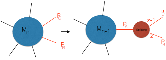
Figure 1: The scattering amplitudes $M_{n}$ involving tensorgluons can be used to extract the splitting amplitudes $Split(h_{B},h_{C},h_{A})$ considering the limit when two neighbouring particles become collinear, $p_{B}\parallel p_{C}$,   $p_{B}=zp_{A},~{}p_{C}=(1-z)p_{A}$,   $p^{2}_{A}\rightarrow 0$ and $z$ describes the longitudinal momentum sharing with the corresponding behaviour of spinors $\lambda_{B}=\sqrt{z}\lambda_{A},~{}~{}~{}\lambda_{C}=\sqrt{1-z}\lambda_{A}.$

The same splitting probabilities can be extracted directly by considering of-mass-shell decay of the particle A. It describes the probability of finding a particle B inside a particle A with fraction z of the longitudinal momentum of A and radiation of the third particle C with fraction $(1-z)$ of the longitudinal momentum of A [13]:

$$P^{C}_{BA}(z)={1\over 2}z(1-z)\sum_{helicities}{|M_{A\rightarrow B+C}|^{2}\over p^{2}_{\perp}},$$ (2.5)

where a sum is over the helicities of B and C and the average over the helicity of A if one is interested in unpolarised splitting probabilities.

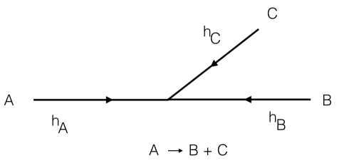
Figure 2: The decay of the tensorgluon A into tensorgluons B and C. The arrows show the directions of the helicities. The corresponding splitting probabilities are defined as $P^{h_{C}}_{h_{B}h_{A}}$.

The important properties of the splitting functions are the symmetries [13, 14, 15, 16, 17] over exchange of the particles $B\leftrightarrow C$ with complementary momenta fraction

$$P^{C}_{BA}(z)=P^{B}_{CA}(1-z)$$ (2.6)

and a crossing relation

$$P^{C}_{AB}(z)=(-1)^{2h_{A}+2h_{B}+1}zP^{C}_{BA}({1\over z}),$$ (2.7)

which emerges because two splitting processes are connected by time reversal $A\leftrightarrow B$.

The splitting probabilities (2.4) were calculated in [5] by using a complex deformation $w$ of the momenta in the triple vertex (2) without breaking the mass shell conditions:

$$p_{1}=(\omega z,w,iw,kz),~{}p_{2}=(\omega(1-z),-w,-iw,k(1-z)),~{}p_{3}=(\omega,0,0,k).$$ (2.8)

The corresponding polarization vectors are to be taken in the form:

$$e^{+}_{1}={1\over\sqrt{2}}({z\over\omega},1,-i,-{z\over k}),~{}e^{+}_{2}={1\over\sqrt{2}}(-{z\over\omega},1,-i,-{z\over k}),~{}e^{-}_{3}={1\over\sqrt{2}}(0,1,-i,0),$$ (2.9)

fulfiling the following relations $p^{2}_{1}=p^{2}_{2}=p^{2}_{3}=p_{1}p_{2}=p_{2}p_{3}=p_{3}p_{1}=p_{1}e^{+}_{1}=p_{2}e^{+}_{2}=p_{3}e^{-}_{3}=0.$ The spinor representation of the momenta (2.8) will take the following form:

$$\lambda_{1}=(\sqrt{(\omega+k)z},0),~{}~{}~{} \tilde{\lambda}_{\dot{1}}=(\sqrt{(\omega+k)z},{2w\over\sqrt{(\omega+k)z}}),$$ (2.10)

$$\lambda_{2}=(\sqrt{(\omega+k)(1-z)},0),~{}~{}~{} \tilde{\lambda}_{\dot{2}}=(\sqrt{(\omega+k)(1-z)},-{2w\over\sqrt{(\omega+k)(1-z)}}),$$

$$\lambda_{3}=(\sqrt{(\omega+k)},0),~{}~{}~{} \tilde{\lambda}_{\dot{3}}=(\sqrt{(\omega+k)},0).$$

It follows that the invariant products $<1,2>=<2,3>=<3,1>=0$ vanish and that

$$[1,2]=-2w{1\over\sqrt{z(1-z)}},~{}~{}~{}[2,3]=2w{1\over\sqrt{1-z}},~{}~{}~{}[3,1]=2w{1\over\sqrt{z}}.$$ (2.11)

Let us consider the interaction vertices (2) of tensorgluons of the spins $A=r$, $C=s$ and $B=s-r+1$, where $s\geq 2r-1$, $r=1,2,3...$. Using the scalar products (2.11) for the vertices (2) one can get:

$$M_{3}(1^{-s},2^{+r},3^{s-r+1}) \propto {[2,3]^{2s+1}\over[1,2]^{2s-2r+1}[3,1]^{2r-1}}=-2w{z^{s}\over(1-z)^{r}}$$

$$M_{3}(1^{-s},2^{s-r+1},3^{+r}) \propto {[2,3]^{2s+1}\over[1,2]^{2r-1}[3,1]^{2s-2r+1}}=-2w{z^{s}\over(1-z)^{s-r+1}}$$

$$M_{3}(1^{+r},2^{s-r+1},3^{-s}) \propto {[1,2]^{2s+1}\over[2,3]^{2r-1}[3,1]^{2s-2r+1}}=-2w{1\over z^{r}(1-z)^{s-r+1}}$$

$$M_{3}(1^{+r},2^{-s},3^{s-r+1}) \propto {[3,1]^{2s+1}\over[2,3]^{2r-1}[1,2]^{2s-2r+1}}=-2w{(1-z)^{s}\over z^{r}}$$

$$M_{3}(1^{s-r+1},2^{+r},3^{-s}) \propto {[1,2]^{2s+1}\over[3,1]^{2r-1}[2,3]^{2s-2r+1}}=-2w{1\over z^{s-r+1}(1-z)^{r}}$$

$$M_{3}(1^{s-r+1},2^{-s},3^{+r}) \propto {[3,1]^{2s+1}\over[1,2]^{2r-1}[2,3]^{2s-2r+1}}=-2w{(1-z)^{s}\over z^{s-r+1}}.$$ (2.12)

These amplitudes can be written in a unified form as

$$M_{3}(h_{B},h_{C},h_{A})\propto{-2w\over z^{h_{B}}(1-z)^{h_{C}}},~{}~{}h_{B}+h_{C}+h_{A}=1.$$ (2.13)

Considering the transversal momentum $p_{\perp}$ in (2.5) to be proportional to the deformation parameter $p_{\perp}\propto w$ one can get the following expression for splitting probabilities:

$$P(z)={1\over 2}z(1-z)|M_{3}|^{2}{1\over|w|^{2}},$$

and then, by using (2), the following set of splitting probabilities [5, 6]:

$$P^{s}_{s-r+1,r} = C_{2}(G){(1-z)^{2s+1}\over z^{2s-2r+1}},~{}~{}~{}~{}P^{s-r+1}_{s,r}=C_{2}(G){z^{2s+1}\over(1-z)^{2s-2r+1}}$$

$$P^{s}_{r,s-r+1} = C_{2}(G){(1-z)^{2s+1}\over z^{2r-1}},~{}~{}~{}~{}P^{s-r+1}_{r,s}=C_{2}(G){1\over z^{2r-1}(1-z)^{2s-2r+1}}$$

$$P^{r}_{s,s-r+1} = C_{2}(G){z^{2s+1}\over(1-z)^{2r-1}},~{}~{}~{}~{}P^{r}_{s-r+1,s}=C_{2}(G){1\over z^{2s-2r+1}(1-z)^{2r-1}},$$ (2.14)

where $s\geq 2r-1$, $r=1,2,3...$. The splitting probabilities for $A=r$, $C=s$ and $B=s-r-1$ are:

$$P^{s}_{s-r-1,r} = C_{2}(G){z^{2s-2r-1}\over(1-z)^{2s-1}},~{}~{}~{}~{}P^{s-r-1}_{s,r}=C_{2}(G){(1-z)^{2s-2r-1}\over z^{2s-1}}$$

$$P^{s}_{r,s-r-1} = C_{2}(G){z^{2r+1}\over(1-z)^{2s-1}},~{}~{}~{}~{}P^{s-r-1}_{r,s}=C_{2}(G)z^{2r+1}(1-z)^{2s-2r-1}$$

$$P^{r}_{s,s-r-1} = C_{2}(G){(1-z)^{2r+1}\over z^{2s-1}},~{}~{}~{}~{}P^{r}_{s-r-1,s}=C_{2}(G)z^{2s-2r-1}(1-z)^{2r+1},$$ (2.15)

where $s\geq 2r+1$ $r=1,2,3...$ . The expressions (2), (2) describe all possible splitting probabilities corresponding to the interaction vertices of the generalised YM theory [1, 5, 6, 7, 8, 9] and can be written in a unified form as

$$P^{h_{C}}_{h_{B}h_{A}}={C_{2}(G)\over z^{2h_{B}-1}(1-z)^{2h_{C}-1}},~{}~{}h_{B}+h_{C}+h_{A}=1.$$ (2.16)

The splitting probabilities (2), (2), (2.16) fulfil the symmetry realtions (2.6), (2.7). For completeness we shall present also quark and gluon splitting probabilities [13]:

$$P^{G}_{qq}(z) = C_{2}(R){1+z^{2}\over 1-z},$$

$$P^{q}_{Gq}(z) = C_{2}(R)[{1\over z}+{(1-z)^{2}\over z}],$$ (2.17)

$$P^{q}_{qG}(z) = T(R)[z^{2}+(1-z)^{2}],$$

$$P^{G}_{GG}(z) = C_{2}(G)\left[{1\over z(1-z)}+{z^{4}\over z(1-z)}+{(1-z)^{4}\over z(1-z)}\right],$$

where $C_{2}(G)=N,C_{2}(R)={N^{2}-1\over 2N},T(R)={1\over 2}$ for the SU(N) groups.

Using the splitting probabilities for the tensorgluons (2), (2) one can derive the evolution equations which will take into account a possible emission of tensorgluons in a proton [5, 6]. Introducing the corresponding densities $T_{s}(x,t)$ of tensorgluons (summed over colours) inside a proton in the $P_{\infty}$ frame one can derive the integro-differential equations that describe the $Q^{2}$ dependence of parton densities in this general case. They are [5, 6]:

$${dq_{i}(x,t)\over dt} = {\alpha(t)\over 2\pi}\int^{1}_{x}{dy\over y}[\sum^{2n_{f}}_{j=1}q_{j}(y,t)~{}P_{q_{i}q_{j}}({x\over y})+G(y,t)~{}P_{q_{i}G}({x\over y})],$$ (2.18)

$${dG(x,t)\over dt} = {\alpha(t)\over 2\pi}\int^{1}_{x}{dy\over y}[\sum^{2n_{f}}_{j=1}q_{j}(y,t)~{}P_{Gq_{j}}({x\over y})+G(y,t)~{}P_{GG}({x\over y})+\sum_{s}T_{s}(y,t)~{}P_{GT_{s}}({x\over y})],$$

$${dT_{r}(x,t)\over dt} = {\alpha(t)\over 2\pi}\int^{1}_{x}{dy\over y}[G(y,t)~{}P_{T_{r}G}({x\over y})+\sum_{s}T_{s}(y,t)~{}P_{T_{r}T_{s}}({x\over y})].$$

The $\alpha(t)$ is the running coupling constant ($\alpha=g^{2}/4\pi$). In the leading logarithmic approximation $\alpha(t)$ is of the form

$${\alpha\over\alpha(t)}=1+b~{}\alpha~{}t~{}~{},$$ (2.19)

where $\alpha=\alpha(0)$ and $b$ is the one-loop Callan-Symanzik coefficient. The densities of the quarks and of gluons are changing because of the standard radiation processes, the density of tensorgluons changes because there are transitions between them through the splittings which are described by the probabilities (2), (2). In the next section we shall derive the splitting amplitudes for the tensorgluons postulation the Yangian symmetry of the amplitudes.

3 Yangian Symmetry of Parton Splitting Amplitudes

In this section we shall present an alternative derivation of the splitting probabilities for tensorgluons postulating the $s\ell_{4}$ Yangian symmetry of the scattering amplitudes of the tensorgluons [18, 19, 22, 21, 20, 23, 24, 26]. As we shall demonstrate, the splitting amplitudes calculated within the Yangian symmetry approach coincide with (2), (2) and hint to the high symmetry of the generalised Yang-Mills theory amplitudes reminiscent to the symmetries discovered in Yang-Mills theory [18, 19, 21, 20, 22, 23, 24, 26]. This is a surprising and encouraging result because such a high symmetry was not explicitly implemented into the initial formulation [1, 5, 6].

We shall derive the splitting amplitudes $Split(h_{B},h_{C},h_{A})$ from the collinear limit of $s\ell_{4}$ Yangian symmetric amplitudes [22, 23, 26]. The latter are defined as eigenfunctions of the monodromy operator of a $s\ell_{4}$ symmetric integrable spin chain, periodic with $N$ sites, composed of the appropriate $4\times 4$ $L$ matrix operators:

$$T({\bf u})=\prod_{1}^{N}L_{i}(u_{i}^{+},u_{i}),\ \ T({\bf u})M(1,...,N)=E({\bf u})M(1,...,N).$$ (3.20)

The matrix elements of $L_{i}$ are operators being generators of the $s\ell_{4}$ algebra and acting on the variables in $M(1,...,N)$ associated with the point $i=1,...,N$. We use the helicity representation, where these variables are the Weyl spinor components $\lambda_{i,\alpha},\bar{\lambda}_{i,\dot{\alpha}},\alpha=1,2,\dot{\alpha}=1,2$. The dependence on the variables at $i$ is homogeneous in the sense that the dilatation of the spinors $\bar{\lambda}_{i}\to t\bar{\lambda}_{i},\ \lambda_{i}\to t^{-1}\lambda_{i}$ implies for the correlation $M(1,...,N)\to t^{2h_{i}-2}M(1,...,N)$. The degree of homogeneity is related to the spectral parameters as $u_{i}^{+}=u_{i}+2h_{i}-2$. In the helicity representation the matrix elements of $L(u^{+},u)\to Iu+L(0)$ are

$$L(0)=\begin{pmatrix}L_{\alpha,\beta}&L_{\alpha,\dot{\beta}}\cr L_{\dot{\alpha},\beta}&L_{\dot{\alpha},\dot{\beta}}\end{pmatrix},$$

$$L_{\alpha,\beta}=-\lambda_{\alpha}\partial_{\beta},~{}L_{\alpha,\dot{\beta}}=-\lambda_{\alpha}\bar{\lambda}_{\dot{\beta}},~{}L_{\dot{\alpha},\beta}=\partial_{\beta}\bar{\partial}_{\dot{\alpha}},~{}L_{\dot{\alpha},\dot{\beta}}=\bar{\partial}_{\dot{\alpha}}\bar{\lambda}_{\dot{\beta}}.$$

The N-point Yangian symmetric correlator can be identified with the scattering amplitudes, where a particle state related to the leg $i$ is represented by the spinors in the known way, in particular, its momentum is $p_{i,\alpha,\dot{\alpha}}=\sigma^{\mu}_{\alpha,\dot{\alpha}}p_{i,\mu}=\bar{\lambda}_{i,\dot{\alpha}}\lambda_{i,\alpha}$ and the particle type is fixed by substituting the physical helicity value for the parameter $h_{i}$.

We shall consider the particular solutions of the $s\ell_{4}$ invariant amplitude with $N=5$ and $N=4$ particles,

$$M_{5}=\delta^{(4)}(\sum_{1}^{5}\lambda_{p,\alpha}\bar{\lambda}_{p,\dot{\alpha}})$$

$$<12>^{-1+2h_{3}+2h_{5}}<23>^{-1+2h_{1}+2h_{4}}<34>^{-1+2h_{2}+2h_{5}}<45>^{-1+2h_{1}+2h_{3}}<51>^{-1+2h_{2}+2h_{4}}=$$

$$=\delta^{(4)}(\sum_{1}^{5}\lambda_{k,\alpha}\bar{\lambda}_{k,\dot{\alpha}})\ \ \prod_{1}^{5}<i-1,i>^{-1+2h_{i-2}+2h_{i+1}}~{},$$ (3.21)

where the helicities obey the constraint $\sum_{1}^{5}h_{i}=1$ and $h_{i+5}=h_{i}$. In the case $N=4$ we obtain

$$M_{4}=\delta^{(4)}(\sum_{1}^{4}\lambda_{k,\alpha}\bar{\lambda}_{k,\dot{\alpha}})\left(\frac{<12><34>}{<23><41>}\right)^{{\varepsilon}}<12>^{-1}<23>^{1-2h_{2}}<34>^{-1+2h_{1}+2h_{2}}<41>^{1-2h_{1}},$$ (3.22)

where only two helicities are independent $h_{3}=-h_{1},\ \ h_{4}=-h_{2}$ and ${\varepsilon}$ remains as a free parameter. The expressions (3)(3.22) are related to the one formulated in [24, 25] for the deformed Grassmannian of $\mathcal{N}=4$ super Yang-Mills scattering amplitudes.

In order to extract the splitting amplitudes for tensorgluons we shall consider the collinear limit of $M_{5}$ in equation (3) (see Fig.1):

$$p_{i}\to zp,\ \ p_{i+1}\to(1-z)p,\ \ \lambda_{i}\to\sqrt{z}\lambda_{p},\ \ \lambda_{i+1}\to\sqrt{1-z}\lambda_{p}~{}.$$

For the products of helicity variables this means that

$$<i,i+1>\to 0,\ \ <i-1,i>\to<i-1,p>\sqrt{z},\ \ <i+1,i+2>\to<p,i+2>\sqrt{1-z}.$$

The factorisation with a one-particle intermediate state occurs if the exponent at $<i,i+1>$ in (3) is $-1$, that is $h_{i-1}+h_{i+2}=0$ and from the constraint $\sum_{1}^{5}h_{i}=1$ it follows then that

$$h_{i-2}+h_{i}+h_{i+1}=1.$$ (3.23)

In the collinear limit we have (omitting the energy-momentum delta distribution)

$$M_{5}~{}\rightarrow~{}(<i-2,i-1>)^{-1+2h_{i}+2h_{i+2}}(<i-1,p>\sqrt{z})^{-1+2h_{i-2}+2h_{i+1}}<i,i+1>^{-1}$$

$$(<p,i+2>\sqrt{1-z})^{-1+2h_{i}+2h_{i-2}}<i+2,i-2>^{-1+2h_{i+1}+2h_{i-1}}.$$

The last expression has a factorised form:

$$M_{5}\to M_{4}<i,i+1>^{-1}Split(h_{i},h_{i+1},h_{p}),$$ (3.24)

where the first factor coincides with the 4-point amplitude (3.22):

$$M_{4}=<i-2,i-1>^{-1+2h_{i}+2h_{i+2}}<i-1,p>^{-1+2h_{i-2}+2h_{i+1}}$$

$$<p,i+2>^{-1+2h_{i}+2h_{i-2}}<i+2,i-2>^{-1+2h_{i+1}+2h_{i-1}}=$$

$$\left(\frac{<i-2,i-1><p,i+2>}{<i-1,p><i+2,i-2>}\right)^{2h_{i}-2}<i-2,i-1>^{1-2h_{i-1}}<i-1,p>^{-1}$$

$$<p,i+2>^{1+2h_{i-2}}<i+2,i-2>^{-1-2h_{i-2}+2h_{i-1}},$$

if one relables the indices $1,2,3,4\to i-1,p,i+2,i-2$ and takes ${\varepsilon}\to 2-2h_{i}$. The last factor is

$$(\sqrt{z})^{-1+2h_{i-2}+2h_{i+1}}(\sqrt{1-z})^{-1+2h_{i}+2h_{i-2}}=\sqrt{z(1-z)}z^{-h_{i}}(1-z)^{-h_{i+1}},$$ (3.25)

where we used the relations $2h_{i+1}+2h_{i-2}=2-2h_{i}$ and $2h_{i}+2h_{i-2}=2-2h_{i+1}$, which follow from (3.23). Thus we were able to extract the splitting amplitude for tensorgluons which has therefore the following elegant form:

$$Split(h_{i},h_{i+1},h_{p})=\frac{\sqrt{z(1-z)}}{z^{h_{i}}(1-z)^{h_{i+1}}}.$$ (3.26)

The helicity of the intermediate state is denoted by $h_{p}=h_{i-2}$ and obeys the relation (3.23) $h_{p}+h_{i}+h_{i+1}=1.$ This condition coincides with the dimensionless condition on the interaction vertices of the generalised Yang-Mills theory (2.2), and here it appears as a consequence of the conformal invariance of the three-particle interaction vertices. If one starts instead with the amplitudes corresponding to the parity reflected particles, then we shall obtain that the splitting amplitudes fulfil the alternative constrain $\sum h_{i}=-1$. Introducing the sign symbol $\eta=\pm 1$ we can formulate both cases in one expression as

$$Split(h_{i},h_{i+1},h_{p})=\frac{\sqrt{z(1-z)}}{z^{\eta h_{i}}(1-z)^{\eta h_{i+1}}},\ \ h_{i}+h_{i+1}+h_{p}=\eta,$$ (3.27)

and for the splitting probability (2.4) we shall get

$$P^{h_{C}}_{h_{B}h_{A}}={1\over z^{2\eta h_{B}-1}(1-z)^{2\eta h_{C}-1}},~{}~{}~{}h_{C}+h_{B}+h_{A}=\eta.$$ (3.28)

It is interesting to notice that the splitting probabilities (2),(2) and (3.28) can be represented in the following symmetric form:

$$P^{h_{C}}_{h_{B}h_{A}}={k_{B}k_{C}k_{A}\over k_{B}^{2\eta h_{B}}k_{C}^{2\eta h_{C}}k_{A}^{2\eta h_{A}}},$$ (3.29)

where the one-dimensional light-cone momenta are defined as in (2.8): $k_{A}=1,~{}k_{B}=z,~{}k_{C}=(1-z)$. In the subsequent sections this expression will be rigorously derived as the light-cone momentum factor of the $s\ell_{2}$ Yangian symmetric amplitude in the two-dimensional helicity representation $h_{i}$ of the solution of the $s\ell_{2}$ version of the equation (3.20) [26].

4 SUSY Symmetry of the Splitting Amplitudes

In the supersymmetric QCD the splitting amplitudes and probabilities fulfil supersymmetric relations which were established in [43, 44, 45]. These ${\cal N}=1$ Kounnas-Ross relations are between splitting probabilities $P_{BA}$ of the members of the supersymmetric multiplets consisting of the matter supermultiplet of quarks $(q_{i})$ and squarks $(s_{i},t_{i})$ and of the vector supermultiplet of gluons $(G)$ and gluinos $(\lambda)$:

$$P_{GG}+P_{\lambda G}=P_{G\lambda}+P_{\lambda\lambda}$$

$$P_{Gq}+P_{\lambda q}=P_{Gs}+P_{\lambda s}$$

$$P_{qG}+P_{sG}=P_{q\lambda}+P_{s\lambda}$$

$$P_{qq}+P_{sq}=P_{qs}+P_{ss}.$$ (4.30)

The first relation is well known from the standard QCD when the quarks are in the adjoint representations of SU(3) [14].

It is interesting to check if the high spin evolution kernels $P^{h_{C}}_{h_{B}h_{A}}$ fulfil generalised ${\cal N}=1$ supersymmetry relations. As we shall demonstrate, the splitting probabilities fulfil the $N=1$ SUSY relations hinting to the fact that the underlying theory can be formulated in an explicit supersymmetric manner. Indeed, considering the supermultiplets $(1,1/2)$ and $(s,s-1/2)$ we shall get the relations including the gluons, gluinos and tensorgluons with their partners tensorgluionos:

$$P^{1/2}_{s(s-1/2)}+P^{1}_{(s-1/2)(s-1/2)}=P^{1/2}_{(s-1/2)s}+P^{1}_{ss}.$$ (4.31)

For the corresponding polarisation kernels we shall have the following expressions (2),(2), (3.28):

$$P^{1/2}_{s^{-}(s-1/2)^{+}}=0,~{}~{}P^{1}_{(s-1/2)^{-}(s-1/2)^{+}}={z^{2s}\over 1-z},~{}~{}P^{1/2}_{(s-1/2)^{-}s^{+}}=z^{2s},~{}~{}P^{1}_{s^{-}s^{+}}={z^{2s+1}\over 1-z};~{}~{}~{}~{}~{}~{}~{}~{}~{}~{}~{}$$ (4.32)

$$P^{1/2}_{s^{+}(s-1/2)^{-}}={1\over z^{2s-1}},P^{1}_{(s-1/2)^{+}(s-1/2)^{-}}={1\over z^{2s-2}(1-z)},P^{1/2}_{(s-1/2)^{+}s^{-}}=0,P^{1}_{s^{+}s^{-}}={1\over z^{2s-1}(1-z)},$$

and, as one can see, each set of these polarisation kernels fulfils the ${\cal N}=1$ relation (4.31). Let us also consider two arbitrary supermultiplets $(s,s-1/2)$ and $(r,r-1/2)$. For these supermultiplets the ${\cal N}=1$ SUSY relation has the following generalised Kounnas-Ross form:

$$P^{s-r+1/2}_{r(s-1/2)}+P^{s-r+1}_{(r-1/2)(s-1/2)}=P^{s-r+1/2}_{(r-1/2)s}+P^{s-r+1}_{rs}.$$ (4.33)

Calculating the corresponding splitting kernels we shall get

$$P^{(r-s+1/2)^{+}}_{r^{-}(s-1/2)^{+}}=0,~{}~{} P^{(r-s+1)^{+}}_{(r-1/2)^{-}(s-1/2)^{+}}={z^{2r}\over(1-z)^{2r-2s+1}},~{}$$ (4.34)

$$P^{(r-s+1/2)^{+}}_{(r-1/2)^{-}s^{+}}={z^{2r}\over(1-z)^{2r-2s}},~{}~{} P^{(r-s+1)^{+}}_{r^{-}s^{+}}={z^{2r+1}\over(1-z)^{2r-2s+1}};$$

$$P^{(s-r+1/2)^{+}}_{r^{+}(s-1/2)^{-}}={1\over z^{2r-1}(1-z)^{2s-2r}},~{}~{} P^{(s-r+1)^{+}}_{(r-1/2)^{+}(s-1/2)^{-}}={1\over z^{2r-2}(1-z)^{2s-2r+1}},~{}$$

$$P^{(s-r+1/2)^{+}}_{(r-1/2)^{+}s^{-}}=0,~{}~{} P^{(s-r+1)^{+}}_{r^{+}s^{-}}={1\over z^{2r-1}(1-z)^{2s-2r+1}}$$

and, as one can see, both sets of polarisation kernels fulfil the supersymmetry relation (4.33).

In the next section we shall consider the amplitudes which are the solution of the $s\ell_{2}$ version of Yangian symmetry (3.20) obtained in [26]. These amplitudes represent a longitudinal, two-dimensional reduction [12] of the four-dimensional $s\ell_{4}$ symmetric amplitudes and, as we shall see, the alternative derivation of the splitting probabilities will coincide with the one presented above but has the advantage to represent the results in a more symmetric form.

5 $s\ell_{2}$ Symmetries of the splitting amplitudes

We notice that the splitting amplitude can be regarded as a result of a particular substitution in the function of 3 one-dimensional light-cone momenta $k_{1},k_{2},k_{3},k_{1}+k_{2}+k_{3}=0$,

$$\phi(a_{1},a_{2},a_{3};k_{1},k_{2},k_{3})=(k_{1}k_{2}k_{3})^{\frac{1}{2}}k_{1}^{-\eta a_{1}}k_{2}^{-\eta a_{2}}k_{3}^{-\eta a_{3}},\ \ \ \sum a_{i}=\frac{1}{2}\eta$$ (5.35)

$$Split(h_{1},h_{2},h_{3};z)=\phi(h_{1},h_{2},h_{3}-\frac{1}{2}\eta;z,1-z,-1).$$

The parton splitting probabilities are calculated as squares of the corresponding splitting amplitudes. The helicities refer to ingoing momenta, i.e. $h_{1},h_{2}$ are opposite to their physical values in the decay $3\to 1+2$:

$$P_{h_{1}\ h_{3}}^{h_{2}}(z)=Split^{2}(h_{1},h_{2},h_{3};z)=\phi^{2}(h_{1},h_{2},h_{3}-\frac{1}{2}\eta;-z,-1+z,1).$$

The expressions for the parton splitting probabilities given in sect. 2 are reproduced.

The simple expression for $\phi(a_{1},a_{2},a_{3};k_{1},k_{2},k_{3})$ results in a number of trivial relations which result through the above substitutions in well known relations of the parton kernels with obvious physical interpretations. This expression can be obtained as the light-cone momentum factor in the $s\ell_{2}$ Yangian symmetric 3-point function in the 2-dimensional analogon of the helicity representation. The latter can be derived as a solution of the $s\ell_{2}$ version of (3.20), as explained in [26]. The explicit form of the $L$ matrix (in the case $\eta=+1$) is $L(u^{+},u)\to Iu+L(0)$

$$L(0)=\begin{pmatrix}S^{0}&S^{-}\cr S^{+}&-S^{0}\end{pmatrix},$$

$$S^{0}=-k\partial_{k},S^{-}=-k,S^{+}=\frac{1}{k}(k\partial_{k}+a-\frac{1}{2})(k\partial_{k}-a-\frac{1}{2})$$

$S^{b},b=0,\pm$ obey the $s\ell_{2}$ Lie algebra relations. Indeed, the 3-point function $\phi$ is determined by the following conditions:

$$(S_{1}^{b}+S_{2}^{b}+S_{3}^{b})\phi~{}\delta(\sum k_{i})=0,\ b=0,\pm.$$

We consider some relations for the symmetric 3-point function and their implications for the splitting probabilities. The relation of parity symmetry for flipping all helicities is obvious in this form, because $\phi(a_{1},a_{2},a_{3};k_{1},k_{2},k_{3})=\phi(-a_{1},-a_{2},-a_{3};k_{1},k_{2},k_{3})$ implies

$$P_{h_{1}\ h_{3}}^{h_{2}}(z)=P_{-h_{1}\ -h_{3}}^{-h_{2}}(z).$$

Further the crossing relations for the exchange of the helicity labels at $P_{h_{2}\ h_{3}}^{h_{1}}(z)$ follow easily from $\phi(a_{1},a_{2},a_{3};k_{1},k_{2},k_{3})=\phi(a_{2},a_{1},a_{3};k_{2},k_{1},k_{3}),~{}~{}\phi(a_{2},a_{1},a_{3};k_{1},k_{2},k_{3})=\phi(a_{1},a_{2},a_{3};k_{2},k_{1},k_{3})$. Indeed, the first relation results in

$$P_{h_{2}\ h_{3}}^{h_{1}}(z)=P_{h_{1}\ h_{3}}^{h_{2}}(1-z).$$

The second relation results in

$$P_{h_{3}\ h_{1}}^{h_{2}}(z)=\pm\ zP_{h_{1}\ h_{3}}^{h_{2}}(\frac{1}{z}).$$

The last relation is obtained by substituting $z=-\frac{k_{1}}{k_{2}},1-z=-\frac{k_{3}}{k_{1}}$ and using $\eta(h_{1}+h_{2}+h_{3})=\frac{1}{2},$ . As an intermediate step we rewrite $\phi$ by using the constraints on the sum of momenta and the sum of parameters $a_{i}$ as

$$\phi(a_{1},a_{2},a_{3};k_{1},k_{2},k_{3})=(k_{1}k_{2}k_{3})^{\frac{1}{2}}k_{1}^{-\frac{1}{2}}(\frac{k_{2}}{k_{1}})^{-\eta a_{2}}(-1-\frac{k_{2}}{k_{1}})^{-\eta a_{3}}.$$

In this way we reproduce the well known crossing relations for the parton splitting probabilities [13, 14]. In this representation we have supersymmetry relations due to momentum conservation. The shift of the parameter $a_{i}$ by $-\frac{1}{2}\eta$ results in an extra factor $k_{i}$, therefore

$$\phi^{2}(a_{1}-\frac{1}{2}\eta,a_{2},a_{3};k_{1},k_{2},k_{3})+\phi^{2}(a_{1},a_{2}-\frac{1}{2}\eta,a_{3};k_{1},k_{2},k_{3})+$$

$$\phi^{2}(a_{1},a_{2},a_{3}-\frac{1}{2}\eta;k_{1},k_{2},k_{3})=\phi^{2}(a_{1},a_{2},a_{3};k_{1},k_{2},k_{3})\ (k_{1}+k_{2}+k_{3})=0.$$ (5.36)

We rewrite this equation in terms of the splitting amplitudes as

$$Split^{2}(h_{1}-\frac{1}{2}\eta,h_{2},h_{3}+\frac{1}{2}\eta;z)+Split^{2}(h_{1},h_{2}-\frac{1}{2}\eta,h_{3}+\frac{1}{2}\eta;z)+Split^{2}(h_{1}+h_{2},h_{3};z)=0$$

and obtain a non-trivial relation for the splitting probabilities which can be related to supersymmetry, because it involves parton helicities differing by $\frac{1}{2}$:

$$P_{h_{1}h_{3}}^{h_{2}}(z)-P_{h_{1}-\frac{1}{2}\eta,h_{3}+\frac{1}{2}\eta}^{h_{2}}(z)-P_{h_{1},h_{3}+\frac{1}{2}\eta}^{h_{2}-\frac{1}{2}\eta}(z)=0.$$ (5.37)

The signs appear in turning from the incoming convention for the momenta to the physical situation $3\to 1+2$. By the substitution $h_{3}+\eta\frac{1}{2}\to h_{3},~{}h_{1}-\eta\frac{1}{2}\to h_{1}$ we obtain another form of the same relation:

$$P_{h_{1},h_{3}}^{h_{2}}(z)+P_{h_{1}+\frac{1}{2}\eta,h_{3}}^{h_{2}-\frac{1}{2}\eta}(z)-P_{h_{1}+\frac{1}{2}\eta,h_{3}-\frac{1}{2}\eta}^{h_{2}}(z)=0.$$ (5.38)

The parton scale evolution involving the doublets of helicities $(h_{3},h_{3}-\frac{1}{2})$, $(h_{1},h_{1}+\frac{1}{2})$ is supersymmetric if the following relation holds:

$$P_{h_{1},h_{3}-\frac{1}{2}}+P_{h_{1},h_{3}}=P_{h_{1}+\frac{1}{2},h_{3}-\frac{1}{2}}+P_{h_{1}+\frac{1}{2},h_{3}}.$$ (5.39)

Here the helicities $h_{2}$ of the exchange parton are summed over

$$P_{h_{1},h_{3}}=P_{h_{1},h_{3}}^{+1-h_{1}-h_{3}}+P_{h_{1},h_{3}}^{-1-h_{1}-h_{3}}=$$

$$\frac{z}{1-z}\left[\frac{z^{2h_{1}}}{(1-z)^{2(h_{3}+h_{1})}}+\frac{(1-z)^{2(h_{1}+h_{3})}}{z^{2h_{1}}}\right].$$

In the above supersymmetry relation thus the helicity values for $h_{2}$ are $h_{+}=+1-h_{1}-h_{3},h_{-}=-1-h_{1}-h_{3},h_{+}\pm\frac{1}{2},h_{-}\pm\frac{1}{2}$. Substituting this into the Susy relation (5.39) we would have

$$(P_{h_{1},h_{3}-\frac{1}{2}}^{h_{-}+\frac{1}{2}}+P_{h_{1},h_{3}-\frac{1}{2}}^{h_{+}+\frac{1}{2}})+(P_{h_{1},h_{3}}^{h_{-}}+P_{h_{1},h_{3}}^{h_{+}})=$$

$$(P_{h_{1}+\frac{1}{2},h_{3}-\frac{1}{2}}^{h_{-}}+P_{h_{1}+\frac{1}{2},h_{3}-\frac{1}{2}}^{h_{+}})+(P_{h_{1}+\frac{1}{2},h_{3}}^{h_{-}-\frac{1}{2}}+P_{h_{1}+\frac{1}{2},h_{3}}^{h_{+}-\frac{1}{2}}).$$

We show that this cannot be valid without restriction. We write (5.37) for $\eta=-1$ and (5.38) for $\eta=+1$.

$$P_{h_{1},h_{3}}^{h_{2}}(z)-P_{h_{1}+\frac{1}{2},h_{3}-\frac{1}{2}}^{h_{2}}(z)-P_{h_{1},h_{3}-\frac{1}{2}}^{h_{2}+\frac{1}{2}\eta}(z)=0,\ \ \ h_{2}=-1-h_{1}-h_{3}=h-$$

$$P_{h_{1},h_{3}}^{h_{2}}(z)+P_{h_{1}+\frac{1}{2},h_{3}}^{h_{2}-\frac{1}{2}}(z)-P_{h_{1}+\frac{1}{2},h_{3}-\frac{1}{2}}^{h_{2}}(z)=0,\ \ \ h_{2}=+1-h_{1}-h_{3}=h_{+}$$

The sum of these relations reproduces the supersymmetry relation (5.39) if the contributions with $h_{2}=h_{-}-\frac{1}{2}$ and $h_{2}=h_{+}+\frac{1}{2}$ are excluded.

6 Conclusion

The aim of this article was to suggest an alternative derivation of the splitting probabilities for tensorgluons postulating the infinite dimensional Yangian symmetry of the scattering amplitudes of the tensorgluons. As we demonstrated, the splitting probabilities calculated within the Yangian symmetry approach coincide with the earlier calculations, which were based on the BCFW recursion relations and were hinting to the high symmetry of the generalised Yang-Mills theory amplitudes reminiscent to the symmetries discovered in Yang-Mills theory. The splitting probabilities have the following highly symmetric and universal form:

$$P^{h_{C}}_{h_{B}h_{A}}={1\over z^{2\eta h_{B}-1}(1-z)^{2\eta h_{C}-1}},~{}~{}~{}h_{C}+h_{B}+h_{A}=\eta=\pm 1.$$ (6.40)

The formula describes all known splitting probabilities found earlier in QFT (2) and generalised Yang-Mills theory (2), (2). It describes splitting probabilities for integer and half-integer spin particles. This is a surprising and encouraging result because such a high symmetry was not explicitly implemented into the initial formulation. We have demonstrated that the splitting probabilities (6.40) fulfil the generalised Kounnas-Ross supersymmetry $N=1$ SUSY relations (4.33) hinting to the fact that the underlying theory can be formulated in an explicit supersymmetric manner [10].

One of us, G.S., would like to thank the Institute of Theoretical Physics of the Leipzig University for hospitality, where part of this work was completed. This work was supported in part by the Alexander von Humboldt Foundation. G.S. was also supported in part by the Marie Skĺodowska-Curie Grant Agreement No 644121.

.

References

- [1] G. Savvidy, Asymptotic freedom of non-Abelian tensor gauge fields, Phys. Lett. B 732 (2014) 150.
- [2] D. J. Gross and F. Wilczek, Asymptotically Free Gauge Theories. 1, Phys. Rev. D 8 (1973) 3633.
- [3] D. J. Gross and F. Wilczek, Asymptotically Free Gauge Theories. 2., Phys. Rev. D 9 (1974) 980.
- [4] H. D. Politzer, Reliable Perturbative Results For Strong Interactions?, Phys. Rev. Lett. 30, 1346 (1973).
- [5] G. Savvidy, Tensor gluons and proton structure, Theor. Math. Phys. 182 (2015) no.1, 114 [Teor. Mat. Fiz. 182 (2014) no.1, 140] doi:10.1007/s11232-015-0250-x [arXiv:1406.5334 [hep-ph]].
- [6] G. Savvidy, Generalisation of the Yang-Mills Theory, Int. J. Mod. Phys. A 31 (2016) no.01, 1630003 doi:10.1142/S0217751X16300039, 10.1142/9789814725569-0015 [arXiv:1511.00274 [hep-th]].
- [7] G. Savvidy, Non-Abelian tensor gauge fields: Generalization of Yang-Mills theory, Phys. Lett. B 625 (2005) 341
- [8] G. Savvidy, Non-abelian tensor gauge fields. I, Int. J. Mod. Phys. A 21 (2006) 4931;
- [9] G. Savvidy, Non-abelian tensor gauge fields. II, Int. J. Mod. Phys. A 21 (2006) 4959;
- [10] I. Antoniadis, L. Brink and G. Savvidy, Extensions of the Poincare group, J. Math. Phys. 52 (2011) 072303 doi:10.1063/1.3607971 [arXiv:1103.2456 [hep-th]].
- [11] G. Savvidy, Extension of the Poincaré Group and Non-Abelian Tensor Gauge Fields, Int. J. Mod. Phys. A 25 (2010) 5765 [arXiv:1006.3005 [hep-th]].
- [12] J. D. Bjorken and E. A. Paschos, Inelastic Electron Proton and gamma Proton Scattering, and the Structure of the Nucleon, Phys. Rev. 185 (1969) 1975.
- [13] G. Altarelli and G. Parisi, Asymptotic Freedom in Parton Language, Nucl. Phys. B 126 (1977) 298.
- [14] Y. L. Dokshitzer, Calculation of the Structure Functions for Deep Inelastic Scattering and e+ e- Annihilation by Perturbation Theory in Quantum Chromodynamics., Sov. Phys. JETP 46 (1977) 641 [Zh. Eksp. Teor. Fiz. 73 (1977) 1216].
- [15] V. N. Gribov and L. N. Lipatov, Deep inelastic e p scattering in perturbation theory, Sov. J. Nucl. Phys. 15 (1972) 438 [Yad. Fiz. 15 (1972) 781].
- [16] V. N. Gribov and L. N. Lipatov, e+ e- pair annihilation and deep inelastic e p scattering in perturbation theory, Sov. J. Nucl. Phys. 15 (1972) 675 [Yad. Fiz. 15 (1972) 1218].
- [17] L. N. Lipatov, The parton model and perturbation theory, Sov. J. Nucl. Phys. 20 (1975) 94 [Yad. Fiz. 20 (1974) 181].
- [18] J. M. Drummond, J. M. Henn and J. Plefka, Yangian symmetry of scattering amplitudes in N=4 super Yang-Mills theory, JHEP 0905 (2009) 046 doi:10.1088/1126-6708/2009/05/046 [arXiv:0902.2987 [hep-th]].
- [19] J. M. Drummond, J. Henn, G. P. Korchemsky and E. Sokatchev, Dual superconformal symmetry of scattering amplitudes in N=4 super-Yang-Mills theory, Nucl. Phys. B 828 (2010) 317 doi:10.1016/j.nuclphysb.2009.11.022 [arXiv:0807.1095 [hep-th]].
- [20] N. Arkani-Hamed, J. L. Bourjaily, F. Cachazo, A. B. Goncharov, A. Postnikov and J. Trnka, Scattering Amplitudes and the Positive Grassmannian, arXiv:1212.5605 [hep-th].
- [21] N. Arkani-Hamed, J. L. Bourjaily, F. Cachazo, S. Caron-Huot and J. Trnka, The All-Loop Integrand For Scattering Amplitudes in Planar N=4 SYM, JHEP 1101 (2011) 041 doi:10.1007/JHEP01(2011)041 [arXiv:1008.2958 [hep-th]].
- [22] D. Chicherin and R. Kirschner, Yangian symmetric correlators, Nucl. Phys. B 877 (2013) 484 doi:10.1016/j.nuclphysb.2013.10.006 [arXiv:1306.0711 [math-ph]].
- [23] D. Chicherin, S. Derkachov and R. Kirschner, Yang-Baxter operators and scattering amplitudes in N=4 super-Yang-Mills theory, Nucl. Phys. B 881 (2014) 467 doi:10.1016/j.nuclphysb.2014.02.016 [arXiv:1309.5748 [hep-th]].
- [24] L. Ferro, T. Lukowski and M. Staudacher, scattering amplitudes and the deformed Grass mannian, Nucl. Phys. B 889 (2014) 192 doi:10.1016/j.nuclphysb.2014.10.012 [arXiv:1407.6736 [hep-th]].
- [25] T. Bargheer, Y. t. Huang, F. Loebbert and M. Yamazaki, Integrable Amplitude Deformations for N=4 Super Yang-Mills and ABJM Theory, Phys. Rev. D 91 (2015) no.2, 026004 doi:10.1103/PhysRevD.91.026004 [arXiv:1407.4449 [hep-th]].
- [26] J. Fuksa and R. Kirschner, Correlators with Yangian symmetry, Nucl. Phys. B 914 (2017) 1 doi:10.1016/j.nuclphysb.2016.10.019 [arXiv:1608.04912 [hep-th]].
- [27] G. Georgiou and G. Savvidy, Production of non-Abelian tensor gauge bosons. Tree amplitudes and BCFW recursion relation, Int. J. Mod. Phys. A 26 (2011) 2537 [arXiv:1007.3756 [hep-th]].
- [28] I. Antoniadis and G. Savvidy, Conformal invariance of tensor boson tree amplitudes, Mod. Phys. Lett. A 27 (2012) 1250103 [arXiv:1107.4997 [hep-th]].
- [29] P. Benincasa and F. Cachazo, Consistency Conditions on the S-Matrix of Massless Particles, arXiv:0705.4305 [hep-th].
- [30] L. J. Dixon, Calculating scattering amplitudes efficiently, arXiv:hep-ph/9601359.
- [31] S. J. Parke and T. R. Taylor, An Amplitude for Gluon Scattering, Phys. Rev. Lett. 56 (1986) 2459.
- [32] E. Witten, Perturbative gauge theory as a string theory in twistor space, Commun. Math. Phys. 252 (2004) 189 [arXiv:hep-th/0312171].
- [33] R. Britto, F. Cachazo, B. Feng and E. Witten, Direct proof of tree-level recursion relation in Yang-Mills theory, Phys. Rev. Lett. 94 (2005) 181602 [arXiv:hep-th/0501052].
- [34] F. Cachazo, P. Svrcek and E. Witten, MHV vertices and tree amplitudes in gauge theory, JHEP 0409 (2004) 006 [arXiv:hep-th/0403047].
- [35] N. Arkani-Hamed and J. Kaplan, On Tree Amplitudes in Gauge Theory and Gravity, JHEP 0804 (2008) 076 [arXiv:0801.2385 [hep-th]].
- [36] F. A. Berends and W. T. Giele, Multiple Soft Gluon Radiation in Parton Processes, Nucl. Phys. B 313 (1989) 595.
- [37] M. L. Mangano and S. J. Parke, Quark - Gluon Amplitudes in the Dual Expansion, Nucl. Phys. B 299 (1988) 673.
- [38] A. K. Bengtsson, I. Bengtsson and L. Brink, Cubic Interaction Terms For Arbitrary Spin, Nucl. Phys. B 227 (1983) 31.
- [39] A. K. Bengtsson, I. Bengtsson and L. Brink, Cubic Interaction Terms For Arbitrarily Extended Supermultiplets, Nucl. Phys. B 227 (1983) 41.
- [40] A. K. H. Bengtsson, I. Bengtsson and N. Linden, Interacting Higher Spin Gauge Fields on the Light Front, Class. Quant. Grav. 4 (1987) 1333.
- [41] R. R. Metsaev, Cubic interaction vertices of massive and massless higher spin fields, Nucl. Phys. B 759 (2006) 147
- [42] T. Adamo, P. Haehnel and T. McLoughlin, Conformal higher spin scattering amplitudes from twistor space, arXiv:1611.06200 [hep-th].
- [43] C. Kounnas and D. A. Ross, Short Distance Structure of Hadrons in Supersymmetric QCD, Nucl. Phys. B 214 (1983) 317. doi:10.1016/0550-3213(83)90665-X
- [44] S. K. Jones and C. H. Llewellyn Smith, Leptoproduction of Supersymmetric Particles, Nucl. Phys. B 217 (1983) 145. doi:10.1016/0550-3213(83)90082-2
- [45] A. P. Bukhvostov, G. V. Frolov, L. N. Lipatov and E. A. Kuraev, Evolution Equations for Quasi-Partonic Operators, Nucl. Phys. B 258 (1985) 601. doi:10.1016/0550-3213(85)90628-5