A multiphase Cahn–Hilliard–Darcy model for tumour growth with necrosis
Abstract
We derive a Cahn–Hilliard–Darcy model to describe multiphase tumour growth taking interactions with multiple chemical species into account as well as the simultaneous occurrence of proliferating, quiescent and necrotic regions. Via a coupling of the Cahn–Hilliard–Darcy equations to a system of reaction-diffusion equations a multitude of phenomena such as nutrient diffusion and consumption, angiogenesis, hypoxia, blood vessel growth, and inhibition by toxic agents, which are released for example by the necrotic cells, can be included. A new feature of the modelling approach is that a volume-averaged velocity is used, which dramatically simplifies the resulting equations. With the help of formally matched asymptotic analysis we develop new sharp interface models. Finite element numerical computations are performed and in particular the effects of necrosis on tumour growth is investigated numerically.
Key words. multiphase tumour growth, phase field model, Darcy flow, necrosis, cellular adhesion, matched asymptotic expansions, finite element computations
AMS subject classification. 92B05, 35K57, 35R35, 65M60
1 Introduction
The morphological evolution of cancer cells, driven by chemical and biological mechanisms, is still poorly understood even in the simplest case of avascular tumour growth. It is well-known that in the avascular stage, initially homogeneous tumour cells will eventually develop heterogeneity in their growth behaviour. For example, quiescent cells appear when the tumour reaches a diffusion-limited size, where levels of nutrients, such as oxygen, are too low to support cell proliferation, and necrotic cells develop when the nutrient density drops further. It is expected that angiogenic factors are secreted by the quiescent tumour cells to induce the development of a capillary network towards the tumour and deliver much required nutrients for proliferation [51]. But it has also been observed (experimentally [46] and in numerical simulations [10, 12]), that the tumour exhibits morphological instabilities, driven by a combination of chemotactic gradients and inhomogeneous proliferation, which allows the interior tumour cells to access nutrients by increasing the surface area of the tumour interface.
In this paper, we propose a multi-component diffuse interface model for modelling heterogeneous tumour growth. We consider types of cells, with chemical species. Similar in spirit to Ambrosi and Preziosi [2] (see also [4, 19, 50]), we model each of the different cell types as inertia-less fluids, and each of the chemical species can freely diffuse and may be subject to additional mechanisms such as chemotaxis and active transport. In the diffuse interface methodology, interfaces between different components are modelled as thin transition layers, in which the macroscopically distinct components are allowed to mix microscopically. This is in contrast to the sharp interface approach, where the interfaces are modelled as idealised moving hypersurfaces. The treatment of cells as viscous inertia-less fluids naturally leads to a notion of an averaged velocity for the fluid mixture, and we will use a volume-averaged velocity, which is also considered in [1, 23].
From basic conservation laws, we will derive the following multi-component model:
| (1.1a) | ||||
| (1.1b) | ||||
| (1.1c) | ||||
| (1.1d) | ||||
| (1.1e) | ||||
for a vector of volume fractions, i.e., and for , where represents the volume fraction of the th cell type, and for a vector , with representing the density of the th chemical species. The velocity is the volume-averaged velocity, is the pressure, is the vector of chemical potentials associated to , and and denote the partial derivatives of the chemical free energy density with respect to and , respectively.
The system (1.1) can be seen as the multi-component variant of the Cahn–Hilliard–Darcy system derived in Garcke et al. [23]. Equation (1.1e) can be viewed as a convection-reaction-diffusion system with a vector of source terms , where for vectors and , the tensor product is defined as for and . The positive semi-definite mobility tensor can be taken as a second order tensor in , or even as a fourth order tensor in , where is the spatial dimension.
Equations (1.1c) and (1.1d) constitute a multi-component convective Cahn–Hilliard system with a vector of source terms and a mobility tensor , which we take to be either a second order tensor in or a fourth order tensor in . Furthermore, we ask that in the former case and in the latter case for any and . These conditions ensure that for if . One example of such a second order mobility tensor is for and so-called bare mobilities , see [17]. The vector is the vector of partial derivatives of a multi-well potential with equal minima at the points , , where is the th unit vector in .
Equation (1.1b) is a generalised Darcy’s law (with permeability ) relating the volume-averaged velocity and the pressure , while in equation (1.1a), and is the sum of the components of the vector of source terms in (1.1c), and (1.1a) relates the gain or loss of volume from the vector of source terms to the changes of mass balance.
Lastly, and are parameters related to the surface tension and the interfacial thickness, respectively. In fact, associated with (1.1) is the free energy
| (1.2) |
where denotes integration with respect to the dimensional Lebesgue measure. The first two terms in the integral account for the interfacial energy (and by extension the adhesive properties of the different cell types), and the last term accounts for the free energy of the chemical species and their interaction with the cells.
As a special case, we consider and , so that we have three cell types; host cells , proliferating tumour cells and necrotic cells , along with one chemical species acting as nutrient, for example oxygen. Then, (1.1e) becomes a scalar equation, with mobility chosen as a scalar function , and the vector becomes a scalar function . In this case, one can consider a chemical free energy density of the form
| (1.3) |
where are constants and is a monotonically decreasing function such that for . The first term of (1.3) will lead to diffusion of the nutrients, and the second term models the chemotaxis mechanism that drives the proliferating tumour cells to regions of high nutrient, which was similarly considered in [10, 11, 23, 31]. The third term shows that it is energetically favourable to be in the necrotic phase when the nutrient density is below . Indeed, when , is positive, and so the term is negative when . Overall we obtain from (1.1) the three-component model
| (1.4a) | ||||
| (1.4b) | ||||
| (1.4c) | ||||
| (1.4d) | ||||
| (1.4e) | ||||
Similar to [23], we define
| (1.5) |
so that (1.4d) becomes
| (1.6) |
which allows us to decouple the chemotaxis mechanism that was appearing in (1.4c) and (1.4d). We point out that it is possible to neglect the effects of fluid flow by sending in the case . By Darcy’s law and , we obtain as , and the above system (1.4) with source terms satisfying transforms into
We now consider the case that tumour cells prefer to adhere to each other instead of the host cells, for general and . More precisely, let denote the volume fraction of the host cells, and is the total volume fraction of the types of tumour cells. Then the following choice of interfacial energy is considered:
| (1.7) |
where is a potential with equal minima at and . Note that (1.7) can be viewed as a function of , i.e., , and it is energetically favourable to have (representing the host tissues) or (representing the tumour as a whole). It holds that the first variation of with respect to , , satisfies
and so, if the chemical free energy density is independent of , the corresponding equations for the chemical potentials for the tumour phases now read as
Then, choosing a second order mobility tensor such that , for , and for a non-negative mobility , the equations for take the form
which resemble the system of equations studied in [8, 9, 20, 54, 56]. Note in particular that only is needed to drive the evolution of , . However, the mathematical treatment of these types of models is difficult due to the fact that the equation for is now a transport equation with a high order source term , and the natural energy identity of the model does not appear to yield useful a priori estimates for . In the case that the mobility is a constant, the existence of a weak solution for the model of [9] has been studied by Dai et al. in [15].
The specific forms of the source terms and will depend on the specific situation we want to model. In our numerical investigations, we will primarily focus on a three-component model consisting of host cells , proliferating tumour cells and necrotic cells in the presence of a quasi-static nutrient , i.e., and . Of biological relevance are the following choices:
| (1.8a) | ||||
| (1.8b) | ||||
| (1.8c) | ||||
| (1.8d) | ||||
The source term (1.8a) models the consumption of nutrients by the proliferating cells at a constant rate . The choice (1.8b) models the proliferation of tumour cells at a constant rate by consuming the nutrient, the apoptosis of the tumour cells at a constant rate , which can be considered as a source term for the necrotic cells, and we assume that the necrotic cells degrade at constant rate . Meanwhile, in (1.8c), any mass gain for the proliferating tumour equals the mass loss by the host cells, and vice versa for the necrotic and proliferating cells. In (1.8d), the functions and are zero except near the vicinity of the interfacial layers. The scaling with is chosen similarly as in [32], which allows the source terms to influence the evolution of the interfaces, see Section 3.4 below for more details.
In (1.1), the parameter is related to the thickness of the interfacial layers, and hence it is natural to ask if a sharp interface model will emerge in the limit . Due to the multi-component nature of (1.1), the sharp interface model consists of equations posed on time-dependent regions for and on the free boundaries for . We refer the reader to Section 3 below for the multi-component sharp interface limit of (1.1), which is too complex to state here.
Instead, we consider the system (1.4) with a quasi-static nutrient (neglecting the left-hand side of (1.4d)), (so that ), , a mobility tensor , and the source term . Then, (1.4) simplifies to
| (1.9a) | ||||
| (1.9b) | ||||
| (1.9c) | ||||
| (1.9d) | ||||
| (1.9e) | ||||
| (1.9f) | ||||
where ,
and we note that and hence diffusion is governed by the difference of chemical potentials, see also [6]. Let us denote , , as the regions of host cells, proliferating tumour and necrotic cells, respectively, along with interfaces and . Note that it makes no sense for the host cells to share a boundary with the necrotic cells, and thus . Then, the sharp interface limit of (1.9) reads as (see Section 3.4 for a derivation)
| (1.10a) | ||||
| (1.10b) | ||||
| (1.10c) | ||||
| (1.10d) | ||||
In the above denotes the unit normal on pointing into or the unit normal on pointing into , is the mean curvature, and are positive constants related the potential , denotes the normal velocity of or , and denotes the jump across the interfaces. Let us point out that for the choice (1.8b) of , equation (1.10a) becomes
and for the choice (1.8c) of , equation (1.10a) becomes
Note that the overall gain or loss in mass is reflected in the equation for , compare [11, §4.6].
In contrast, multi-component models obtained from a degenerate interfacial energy such as (1.7) have simpler sharp interface limits. Due to the fact that (1.7) is a function only of , the asymptotic analysis leads to a sharp interface limit which is defined on two time-dependent regions (tumour) and (host), and one free boundary . In particular, differentiation between the different types of tumour cells is based on the local density of nutrients [40, 41, 42, 57], unlike in (1.10) where an evolution law for the interface between the proliferating and necrotic cells is stated. We refer the reader also to Section 3.5 below for the sharp interface limit of a model with degenerate interfacial energy.
Let us now give a non-exhaustive comparison between the multi-component diffuse interface models in the literature and the model (1.1) we propose in this work.
Interfacial energy/cellular adhesion.
In [8, 9, 20, 37, 38, 54, 56], it is assumed that the different types of tumour cells prefer to adhere to one another instead of the host cells, and thus the degenerate interfacial energy density (1.7) is considered. This is in contrast to Oden et al. [45] and our present work, where the adhesive properties of different cell types are distinct and the total energy (1.2) is considered. Furthermore, we point out that the model of Xu et al. [55] can be seen as a two-phase model (tumour and host cells), which uses an interfacial energy similar to (1.7). But they use a non-conserved phase field equation of Allen–Cahn type, rather than a Cahn–Hilliard equation, to describe the tumour evolution.
Mixture velocity.
Source terms.
Aside from mitosis proportional to the local density of nutrients, and constant apoptosis for the tumour cells, certain sink terms for one cell type become source terms for another, for example the term in (1.8b). It is commonly assumed that the host cells are homeostatic [8, 9, 20, 56, 54], and so the source term for the host cells is zero. In [37, 38], where quiescent cells are also considered, a two-sided exchange between the proliferating cells and the quiescent cells, and a one-sided exchange from quiescent cells to necrotic cells based on local nutrient concentration are included. However, to the best of our knowledge, source terms of the form (1.8d) have not yet been considered in the multi-component setting.
Sharp interface limit.
Out of the aforementioned references, only Wise et al. [54] state a sharp interface limit for a multi-component diffuse interface model with degenerate interfacial energy (1.7).
The remainder of this paper is organised as follows: In Section 2 we derive the diffuse interface model (1.1) from thermodynamic principles. In Section 3 we perform a formal asymptotic analysis to derive the sharp interface limit. In Section 4 we present some numerical simulations for the three-component tumour model derived in this paper.
2 Model derivation
Let us consider a mixture consisting of cell components in an open, bounded domain , . Moreover, we allow for the presence of chemical species in . Let , , denote the actual mass of the matter of the th component per volume in the mixture, and let , be the mass density of a pure component . Then the sum denotes the mixture density (which is not necessarily constant), and we define the volume fraction of component as
| (2.1) |
We expect that physically, and thus . Furthermore we allow for mass exchange between the components, but there is no external volume compartment besides the components, i.e.,
| (2.2) |
For the mixture velocity we consider the volume-averaged velocity
| (2.3) |
where is the individual velocity of component , and we denote the density of the th chemical species as , , where each chemical species is transported by the volume-averaged mixture velocity and a flux , .
2.1 Balance laws
The balance law for the mass of each component reads as
| (2.4) |
where denotes a source/sink term for the th component. Using (2.1) we have
| (2.5) |
Upon adding and using (2.3) and (2.2), we obtain an equation for the volume-averaged velocity:
| (2.6) |
On recalling (2.3), we introduce the fluxes
| (2.7) |
so that from (2.5) we obtain
| (2.8) |
Rewriting the mass balance (2.4) with and upon summing we obtain the following equation for the mixture density:
| (2.9) |
Moreover, by summing (2.7) we obtain the requirement
| (2.10) |
For , we postulate the following balance law for the th chemical species
| (2.11) |
where denotes a source/sink term for the th chemical species, models the transport by the volume-averaged velocity and accounts for other transport mechanisms. It is convenient to introduce the vector form of the balance laws (2.8) and (2.11). Let
| (2.12) | ||||||
and
| (2.13) |
i.e., the th row of is the flux and the th row of is the flux . We recall that the divergence applied to a second order tensor results in a vector in whose th component is the divergence of , that is, . Then, (2.8), (2.11) and (2.6) become
| (2.14) | ||||
| (2.15) |
respectively, where .
2.2 Energy inequality
For , , we define
| (2.16) |
The latter is also known as the Gibbs simplex. The corresponding tangent space can be identified as the space
| (2.17) |
We postulate a general free energy of Ginzburg–Landau form, i.e.,
| (2.18) |
where , and . Here are constants, is a smooth gradient energy density and is a smooth multi-well potential with exactly equal minima at the points , , where is the th unit vector in . In particular, the minima of are the corners of the Gibbs simplex . The first two terms in the integral in (2.18) account for interfacial energy and unmixing tendencies, and the term accounts for the chemical energy of the species and any energy contributions resulting from the interactions between the cells and the chemical species.
Recalling the vector , we now introduce the projection operator to the tangent space as follows:
| (2.19) |
for a vector . For a second order tensor we define the th component of its projection to be
We now derive a diffuse interface model based on a dissipation inequality for the balance laws in (2.14) and (2.15). We point out that balance laws with source terms have been used similarly by Gurtin [28, 29] and Podio-Guidugli [48] to derive phase field and Cahn–Hilliard type equations. These authors used the second law of thermodynamics which in an isothermal situation is formulated as a free energy inequality.
The second law of thermodynamics in the isothermal situation requires that for all volumes , which are transported with the fluid velocity, the following inequality has to hold (see [28, 29, 48] and [30, Chapter 62])
where denotes integration with respect to the dimensional Hausdorff measure, is the outer unit normal to , is an energy flux yet to be specified, and we have postulated that the source terms and carry with them a supply of energy described by
| (2.20) |
for some , and yet to be determined.
Applying the transport theorem and the divergence theorem, we obtain the following local form
| (2.21) |
We now use the Lagrange multiplier method of Liu and Müller ([1, Section 2.2] and [39, Chapter 7]). Let , and denote the Lagrange multipliers for the equations in (2.14) and (2.15), respectively. Then, we require that the following inequality holds for arbitrary , , , , , , , and :
| (2.22) | ||||
Using the identities
and the product rule
| (2.23) |
where for two tensors and , the product is defined as , we arrive at
| (2.24) | ||||
where
We can rewrite the term involving as follows (using the notation ):
Applying the product rule on the term involving we get
Thus, substituting the above into the expression (2.24) we obtain
| (2.25) | ||||
2.3 Constitutive assumptions and the general model
We define the vector of chemical potentials to be
| (2.26) |
and by the definition (2.19) of the projection operator , we have
as and . Furthermore, from (2.10) we find that , and so (2.25) can be simplified to
| (2.27) | ||||
Based on (2.27) we make the following constitutive assumptions,
| (2.28a) | ||||
| (2.28b) | ||||
| (2.28c) | ||||
where and are non-negative second order mobility tensors such that
| (2.29) |
Here, by a non-negative second order tensor , we mean that for all , and if and only if . Recalling the definition of and from (2.13), we see that for , the th component of the fluxes and are given as
Then, the constraint (2.10) requires
| (2.30) |
which is satisfied when the constitutive assumption (2.29) is considered. We point out that one may take as a non-negative fourth order mobility tensor, that is, and if and only if for any second order tensors . If we also consider as a fourth order tensor, then (2.29) becomes
| (2.31) |
and for , the th component of the fluxes and are given as
Note that, from (2.27) and the arbitrariness of , we require the prefactor to vanish. Since and the vector is orthogonal to this leads to the consideration and in (2.28b). We introduce a pressure-like function and choose
| (2.32) |
and, for a positive constant ,
| (2.33) | ||||
We can further simplify (2.33) with the identity:
and hence, (2.33) becomes
| (2.34) |
Thus, the model equations are
| (2.35a) | ||||
| (2.35b) | ||||
| (2.35c) | ||||
| (2.35d) | ||||
| (2.35e) | ||||
where
The constitutive choices above lead to the following energy identity.
Theorem 2.1.
A sufficiently smooth solution to (2.35) fulfills
Proof.
Taking the scalar product of (2.35c) with and integrating over leads to
| (2.36) | ||||
Taking the projection of (2.35d) and the scalar product with , and integrating over leads to
| (2.37) | ||||
where we used the linearity of the projection operator to deduce that . Integrating by parts on the last term of (2.37) leads to
| (2.38) | ||||
Next, taking the scalar product of (2.35e) with and integrating over leads to
| (2.39) | ||||
while taking the scalar product of (2.35b) with and integrating over gives
| (2.40) | ||||
where we used the projection operator to deduce that . Note that
Furthermore, by the definition of the projection operator and the fact that , , it holds that
Thus, adding (2.36), (2.38), (2.39) and (2.40) gives the energy identity. ∎
Remark 2.1.
It follows from Theorem 2.1 that, under the boundary conditions
on , and in the absence of source terms and , the total free energy is non-increasing in time.
2.4 Specific models
2.4.1 Zero velocity and zero excess of total mass
Assuming zero excess of total mass, i.e., , we obtain from (2.35a) that . Then, sending in (2.35b) formally implies that , see also [22, §6] for a rigorous treatment in the two-component case. Then (2.35), with source terms satisfying , can be reduced to
| (2.41a) | ||||
| (2.41b) | ||||
| (2.41c) | ||||
which can be seen as the multiphase analogue of the model considered in [23, §2.4.3]. Note that due to the condition and (2.29) (for second order tensors) or (2.31) (for fourth order tensors), we necessarily have that for all if the initial condition for belongs to .
2.4.2 Choices for the Ginzburg–Landau energy
Typical choices for the gradient part of the free energy are the following
where the constants , are referred to as the gradient energy coefficient of phases and (see [21, 26]). For the potential part, we may consider the following
where denotes the Boltzmann constant, is the absolute temperature, and is a symmetric matrix with zeros on the diagonal and positive definite on . For example, the choice , where is the identity matrix, is used in [5, 26, 44]. One can check that for any . We can also consider obstacle potentials that penalise the order parameter from straying out of the set :
| (2.42) |
Let us also mention potentials of polynomial type, which generalise the quartic double-well potential commonly used in two-phase diffuse interface models. One example is
where are positive constants [25].
2.5 Degenerate Ginzburg–Landau energy
As described in Section 2.2, we may consider a Ginzburg–Landau-type energy of the form
for some , i.e., can be independent of and for any , and is a scalar potential with equal minima at and . In the simplest setting and if the chemical free energy density is independent of , we obtain from (2.35d) that
Together with a mobility tensor such that for some mobility function , we obtain from (2.35c)
Thus, we obtain a Cahn–Hilliard type equation for , while for we have a transport equation with source terms and . This is similar to the situations encountered in [8, 9, 15, 20, 54, 56].
2.6 Mobility tensor
We consider second order mobility tensors which fulfill (2.29). For future analysis and numerical implementations, it is advantageous to consider a mobility that is symmetric and positive semi-definite on , see for instance [3, 17]. In most cases is expected to mainly depend on and our standard choice will be independent of and of the form
| (2.43) |
where , , are the so-called bare mobilities. Here, we assume that the vector is not identically zero on the Gibbs simplex, so that the reciprocal of the sum is well-defined. Summing over in (2.43) shows that (2.29) is satisfied. Furthermore, for any , we have (for notational convenience we write for )
where we have used the relations
In particular, for any , is positive semi-definite.
2.7 Reduction to a two-component tumour model
We assume that the domain consists of proliferating tumour tissue and host tissue in the presence of a chemical species acting as a nutrient for the tumour. Let and , and set
| (2.44) | ||||
together with a scalar mobility
| (2.45) |
which we here assume to be independent of , for the nutrient equation and a second order mobility tensor of the form (2.43) with bare mobilities and . With the help of (2.43) the entries of can be computed as
Then, upon defining a non-negative scalar mobility that is a function of as
| (2.48) |
it can be shown that (2.35) becomes
| (2.49a) | ||||
| (2.49b) | ||||
| (2.49c) | ||||
| (2.49d) | ||||
| (2.49e) | ||||
which coincides with [23, Equation (2.25)]. We refer the reader to [23] for a detailed comparison between (2.49) with other two-component phase field models of tumour growth in the literature.
2.8 Tumour with quiescent and necrotic cells
In this section, we give some examples of source terms for the case where a tumour exhibits a quiescent region and a necrotic region. Let and denote the volume fractions of the host tissue, proliferating tumour cells, quiescent tumour cells and necrotic tumour cells by , , , and , respectively, i.e., .
We assume matched densities, i.e., , and that there are two chemical species present in the domain, i.e., . The first is a nutrient whose concentration is denoted as , and is only consumed by the proliferating and quiescent tumour cells, and the second is a toxic intracellular agent, whose concentration is denoted as . Hence . During necrosis, the cell membrane loses its integrity and toxic agents from the former intracellular compartment flow outwards. We assume that these toxic agents act as growth inhibitors on the surrounding living cells and degrade at a constant rate. Furthermore, we denote by , , the critical concentrations such that
-
•
if , then the proliferating tumour cells will turn quiescent,
-
•
if , then the quiescent tumour cells will undergo necrosis,
-
•
if , then the toxic agents start to inhibit the growth of the living cells.
For the source/sink terms , , we consider
| (2.50a) | ||||
| (2.50b) | ||||
with constant consumption rates , by the proliferating and quiescent cells, respectively, constant release rate of toxic agents by the necrotic cells, and constant degradation rate of the toxic agents. We consider the following free energy density :
| (2.51) |
where denote parameters related to the diffusivity of the nutrient and of the toxic agent, respectively, and can be viewed as a parameter for transport mechanisms such as chemotaxis and active transport. Neglecting the toxic agent, the above form for the free energy density is similar to the one chosen in [23, 31]. In particular, the first two terms of lead to diffusion of the nutrient and toxic agent, respectively, while the third term of will give rise to transport mechanisms that drive the proliferating tumour cells to the regions of high nutrient, and also drive the nutrient to the proliferating tumour cells, see [23] for more details regarding the effects of the third term.
Then, computing and considering to be the second order identity tensor , (2.35e) becomes
| (2.52a) | ||||
| (2.52b) | ||||
For the source terms , we assume that
-
•
the host cells experience apoptosis at a constant rate and are inhibited by the toxic agent at a constant rate , leading to
where denotes the positive part of .
-
•
The proliferating tumour cells grow due to nutrient consumption at a constant rate , experience apoptosis at a constant rate , and are inhibited by the toxic agents at the rate . Furthermore, when falls below , there is a transition to the quiescent cells at a constant rate , but when the nutrient concentration is above , there is a transition from the quiescent cells at a constant rate . Altogether this yields
-
•
The quiescent cells experience apoptosis at a constant rate , and are inhibited by the toxic agent at the rate . Furthermore, aside from the exchange between the proliferating cells and the quiescent cells when the nutrient concentration falls below or is above the critical concentration , there is also a transition to the necrotic cells when falls below . This occurs at a constant rate , and we obtain
-
•
The necrotic cells degrades at a constant rate and there is a transition from the quiescent cells at the rate when falls below . Furthermore, the apoptosis of the proliferating and quiescent cells is a source term for the necrotic cells. This yields
In practice, on the time scale considered, is small and will often be neglected. A unique feature of the necrotic core is reflected in the second term of , which describes a spontaneous degradation of the necrotic core. Physiologically, one would expect that the remains of the necrotic cells are slowly processed by specialised cells, leaving only extracellular liquid behind. Since we do not account for a pure liquid phase in our systems, we obtain a local mass defect due to the disintegration of the necrotic core. For the source terms discussed above, the equation (2.6) for equal densities then becomes
and the disintegration of the necrotic core leads to a sink term for the divergence of the volume-averaged velocity field. Hence one could argue that there are two effects resulting from the existence of a necrotic core which could possibly limit the uncontrolled growth of the tumour colony. On the one hand we have the obvious growth inhibition due to the toxic agents, whereas on the other hand the degradation of the necrotic core draws the growing periphery of the tumour back towards the tumour centre.
2.9 Blood vessels and angiogenic factors
We can introduce angiogenic factors into the system by considering two additional chemical species: blood vessels whose density is denoted as and an angiogenic factor whose concentration is denoted as . Hence . We assume that
-
•
the blood vessels offer a supply of nutrient at a constant rate , which leads to the modification
The new term in models the situation where if the nutrient concentration is below , then additional nutrient is supplied by the blood vessels at a rate . However, if , then the nutrient diffuses into the blood vessels and is transported away from the cells.
-
•
The blood vessels are capable of removing the toxic agents released by the necrotic cells at a constant rate , which leads to the modification
-
•
The angiogenic factor is a chemical species that is released by the quiescent tumour cells at a constant rate due to the lack of nutrient in their surroundings, and it degrades at a constant rate . This leads to
In our model, tumour cells become quiescent as a consequence of a lack of nutrient. Therefore it makes sense to assume that the cells, which are in most need of a reliable vascularisation, are secreting factors which induce the necessary blood vessel growth. This assumption has already been suggested in [7, 14]. A very important example for tumour nutrient is oxygen. It is well known that a lack of this nutrient, hypoxia, is an important stimulus for angiogenesis [51].
-
•
Meanwhile, the angiogenic factor induces angiogenesis and consequently the vessel density around the badly supplied tumour cells increases at a constant rate . There are two ways in which the blood vessels can degrade. The first is a natural process which occurs at a constant rate , and the second is through the overexposure of the toxic agent. That is, the blood vessels degrade at a constant rate when the concentration of the toxic agent is higher than the critical value . These considerations lead to
Similar to Section 2.8, for the choice of the free energy density , we consider
| (2.53) |
The difference between (2.51) and (2.53) is the addition of the terms to model the diffusion of the blood vessel density and the angiogenesis factor, respectively. Computing and taking as the identity tensor in , we arrive at the following system for the chemical species:
| (2.54a) | ||||
| (2.54b) | ||||
| (2.54c) | ||||
| (2.54d) | ||||
We expect that in practice, however choosing to be positive is beneficial for the analytical and numerical treatment of the equations.
An alternative way to model angiogenesis is as follows. One could fix the blood vessel density on the boundary of the domain and assume that blood vessel growth is governed by chemotaxis towards the angiogenic factor, meaning that blood vessels are drawn towards regions with a high concentration of angiogenic factors. In this case, we neglect the first term of , leading to
If we consider the free energy density as in (2.53), with its partial derivative with respect to the vector given as
then we may consider a second order mobility tensor of the form
where is a chemotactic sensitivity to the angiogenic factor. Then, upon computing , this yields the following convection-reaction-diffusion system for the blood vessel density and the angiogenic factor:
The term in the equation for can also be found in the classical models for chemotaxis (see for example [33, 34, 35, 36]). We remark that the above modelling approach is different to that in [20] (see also [11, Section 5.12]), which utilises a random walk model for angiogenesis.
2.10 Three phase model with necrotic cells
In Section 4, we perform numerical simulations of a three-component model, similar to (1.4), consisting of host, proliferating and necrotic cells, along with a single nutrient . Neglecting the quiescent cells and the toxic intracelluar agent , as well as the apoptosis of host cells , the source terms from Section 2.8 now become
where the mass lost by the proliferating cells through apoptosis is equal to the mass gained by the necrotic cells. In the case of equal densities , this yields the vector in (1.8b). Alternatively, we can consider source terms of the form
| (2.55) |
where is a non-negative function satisfying , , and is a parameter measuring the thickness of the interfacial layers, recall (1.2). One such example is , which in the case of equal densities leads to the vector in (1.8d). These source terms are chosen in the spirit of [32] (see also [23, §3.3.2]), where we note that is non-zero only near the vicinity of the interfacial layers, while the scaling with and the specific properties of ensure that these source terms only appear in the equation of motion for the interfaces when we consider the sharp interface limit .
3 Sharp interface asymptotics
Different models have been suggested to describe free boundary problems involving multiphase tumour growth. In particular, the effect of a necrotic core has been studied in [13, 18]. In this section, we will perform a formally matched asymptotic analysis for the phase field model (2.35) in order to derive new free boundary problems for tumour growth. We make the following assumptions:
Assumption 3.1.
-
1.
and for positive constants and .
-
2.
The mass exchange terms and depend only on and , and not on any derivatives.
-
3.
The mobility tensor is a strictly positive and smooth fourth order tensor for all and . Here by a strictly positive fourth order tensor we mean for all second order tensors , , and .
-
4.
is a smooth multi-well potential with equal minima at the points satisfying for . Furthermore, we assume that there exist constants and such that
-
5.
We choose the gradient energy as
-
6.
The mobility tensor for all and is a smooth fourth order tensor such that (2.29) is satisfied and also fulfils for all and .
-
7.
For small , we assume that the domain can be divided into open subdomains , , separated by interfaces , that do not intersect with each other or with the boundary .
-
8.
We assume that there is a family of solutions to (2.35), which are sufficiently smooth and have an asymptotic expansion in in the bulk regions away from the interfaces (the outer expansion), and another expansion in the interfacial regions close to the interfaces (the inner expansion).
Remark 3.1.
In the above assumption, for a domain , , we exclude the possibility of triple junction points in and triple junction lines or quadruple junction points in . Although the method of formally matched asymptotic analysis is able to derive certain boundary/angle conditions for the interfaces at such a triple junction, as the case of junctions is not so relevant for tumour growth we will omit the analysis and refer the reader to [5, 6, 24, 25, 43].
With the above assumptions, (2.35) becomes
| (3.1a) | ||||
| (3.1b) | ||||
| (3.1c) | ||||
| (3.1d) | ||||
| (3.1e) | ||||
The idea of the method is to plug the outer and inner expansions in the model equations and solve them order by order. In addition, we have to define a suitable region where these expansions should match up.
We will use the following notation: and denote the terms resulting from the order outer and inner expansions of (3.1a), respectively. For convenience, we will denote by the variable .
3.1 Outer expansions
We assume that for , the following outer expansions hold:
where to ensure that the constraint is satisfied, we additionally assume that
Note that we can relate the expansions for by means of Taylor’s expansion:
| (3.2) |
To leading order we have
| (3.3) |
The stable solutions to (3.3) are the minima of , that is, , . Thus, to leading order the domain is partitioned into regions corresponding to the stable minima of . We define
Since is the zero tensor in the bulk regions , , we obtain from (3.1a), (3.1b), (3.1c) and (3.1e) to zeroth order in each bulk region:
| (3.4a) | ||||
| (3.4b) | ||||
| (3.4c) | ||||
| (3.4d) | ||||
3.2 Inner expansions and matching conditions
In this section we fix and construct a solution that makes a transition from to across a smoothly evolving hypersurface moving with normal velocity . Let denote the signed distance function to , and set as the rescaled distance variable. Here we use the convention that in and in . Thus the gradient points from to and we may use on as a unit normal .
Let denote a parameterisation of by arclength , and in a tubular neighbourhood of , for smooth functions , we have
In this new -coordinate system, the following change of variables apply (see [1, 27]):
where denotes the surface gradient of on and h.o.t. denotes higher order terms with respect to . In particular, we have
where is the mean curvature of . Moreover, if is a vector-valued function with for in a tubular neighbourhood of , then we obtain
We denote the variables , , , , , in the new coordinate system by , , , , , , respectively. We further assume that they have the following inner expansions:
for such that
to ensure that the constraint is satisfied. Analogous to (3.2), by Taylor’s expansion, we have
| (3.5) |
In order to match the inner expansions valid in the interfacial region to the outer expansions of Section 3.1, we employ the matching conditions, see [27]:
| (3.6) | ||||
| (3.7) | ||||
| (3.8) |
where for and . Here we use the convention that for a vectorial quantity , the right hand side of (3.8) reads as . Moreover, we use the following notation: Let and for with and , we denote the jump of a scalar quantity across the interface by
| (3.9) |
For a vectorial quantity , we define
It will be useful to compute the expansion for the term as follows: For fixed and , we find from the above change of variables formula
where denotes the th component of the surface gradient, i.e., . Plugging in the expansion (where we use to denote the th term of the inner expansion for the th component of ) and using Taylor’s theorem we have
| (3.10) | ||||
where we evaluate the last term at and . Using that
we obtain the expansion for the term . One can also derive a similar expansion for .
3.2.1 Expansions to leading order
To leading order we obtain
| (3.11) |
This is a second order differential equation for , and for each we solve the above ordinary differential equation (in ) with the boundary conditions
| (3.12) |
which then yields a vector-valued function that connects to and hence the values of the phase fields in and . By the assumptions satisfied by in Assumption 3.1, it is shown in Sternberg [53, Lemma, p. 801] that for any , there exists a curve such that and and the Lipschitz continuous function
Let us define as the monotone solution of
and then set
Then, it holds that and
| (3.13) | ||||
It follows that is a candidate solution to the following problem
Computing its Euler–Lagrange equations (subject to the constraint ) yields that
and if we consider
then satisfies (3.11) and (3.12). Furthermore, multiplying (3.11) with , integrating with respect to and applying the matching condition (3.6) to , leads to the so-called equipartition of energy:
and we define the surface energy to be
| (3.14) |
Next, gives
| (3.15) |
Integrating with respect to and using the matching condition (3.6) applied to leads to
| (3.16) |
From and (3.10) we have
| (3.17) |
Multiplying by and summing from to and then integrating with respect to , we obtain from integration by parts and the matching condition (3.7) applied to that
The strict positivity of (in the sense of Assumption 3.1) yields
| (3.18) |
i.e., is independent of . Moreover, integrating (3.18) with respect to and using the matching condition (3.6) applied to gives
| (3.19) |
Meanwhile, from , we have
| (3.20) |
Multiplying by and summing from to , an analysis similar to the above for using the assumptions on yields that
| (3.21) |
Lastly, yields
| (3.22) |
Taking the scalar product with and then integrating with respect to leads to
| (3.23) |
where we used the matching condition (3.6) applied to and the fact that and so . Thanks to the fact that is independent of , we find that
| (3.24) |
Recalling from (3.5), we have
| (3.25) | ||||
and so (3.23) becomes
| (3.26) |
3.2.2 Expansions to first order
To first order, we find from
| (3.27) |
where we used that is only a function of and so is the zero tensor. As , , and hence after multiplying (3.27) with and integrating over we obtain
| (3.28) | ||||
where is the mean curvature of and we have used that . Due to the symmetry of the tensor it holds that
| (3.29) |
Then by integrating by parts we obtain from (3.11) and the matching conditions (3.6), (3.7) applied to that
Using (3.14), (3.24), and (3.25), we obtain from (3.28) the following solvability condition for :
| (3.30) |
Next, thanks to the fact that , to first order we obtain from
| (3.31) |
We note that by the matching condition (3.8) applied to , we have , and hence
From (3.15), is independent of , so integrating (3.31) with respect to and applying the matching condition (3.6) to and (3.8) to gives
| (3.32) |
Similar, thanks to the fact that , we obtain from
| (3.33) |
and upon integrating with respect to we obtain
| (3.34) |
In summary, we obtain the following sharp interface model: In the bulk domains , ,
| (3.35a) | ||||
| (3.35b) | ||||
| (3.35c) | ||||
| (3.35d) | ||||
and on the free boundaries , , with unit normal pointing from to ,
| (3.36a) | ||||
| (3.36b) | ||||
| (3.36c) | ||||
| (3.36d) | ||||
| (3.36e) | ||||
| (3.36f) | ||||
where the surface energy is defined in (3.14).
3.3 Sharp interface limit for a two-component tumour model
We now sketch the argument to recover the sharp interface model [23, Equation (3.49)] from (3.35)-(3.36) for a two-component model of host cells and tumour cells, along with a single nutrient species, recall also Section 2.7. Dropping the subscript from (3.35)-(3.36), we consider (2.44) with
along with the scalar mobility (2.45), and the second order mobility tensor defined in (2.48). Setting and , we obtain
| (3.37a) | |||||
| (3.37b) | |||||
| (3.37c) | |||||
| (3.37d) | |||||
To obtain the free boundary conditions on , let denote the solution to (3.11) that connects to , and let denote the difference between the second and first component of . Then, it holds that and with and . We now derive the ODE which is satisfied by . Taking the difference between the second and first component of (3.11) (noting that the last term on the right-hand side of (3.11) will not contribute to this difference), it holds that satisfies
The unique solution to the above ODE with the boundary conditions and satisfying is the function . With the help of (3.14), we compute the surface energy to be
We observe that the jump conditions (3.36c) and (3.36f) become
respectively, and a short computation shows that
so that (3.36d) becomes . Furthermore, taking the difference between the second and first components of the free boundary conditions (3.36b) and (3.36e), the free boundary conditions on translates to
| (3.38a) | ||||
| (3.38b) | ||||
The resulting sharp interface model coincides with [23, Equation (3.49)].
3.4 Sharp interface limit for (1.9)
In this section, we derive the sharp interface limit of (1.9), so that and , from the general sharp interface model (3.35)-(3.36), where we again drop the subscript . Choosing (1.3) with , and (2.43) with , , we have
so that and . Moreover, defining , and , with interfaces , , we assume that . One can compute that , and thus upon setting
from (3.35c) and (3.35d) (recalling that evolves quasi-statically) we obtain the following outer equations:
Meanwhile, due to the fact that and , we obtain from (3.36a), (3.36b), (3.36c) and (3.36f) that
Furthermore, (3.36d) and (3.36e) simplify to
In the case where source terms of the form (1.8d) are considered, the asymptotic analysis requires a slight modification, which we will briefly sketch below. The multi-component system we study is given by
| (3.39a) | ||||
| (3.39b) | ||||
| (3.39c) | ||||
| (3.39d) | ||||
| (3.39e) | ||||
where we now consider
with scalar functions , . For example, we may choose , for , and , , in order to match with (1.8d).
In the outer expansions, we obtain (3.3) from , which implies that , . Then noting that the source term will not contribute to leading and first order, we obtain from the zeroth order expansions of (3.39a)-(3.39c), (3.39e) the outer equations
For the free boundary conditions on the interface , using the inner expansions, we recover (3.21) from and from we have similarly that is a function only in connecting to . While the rest of the analysis is analogous, the only difference lies in and where now the source term enters. More precisely, from and we have
| (3.40a) | ||||
| (3.40b) | ||||
Using the fact that (from ) and introducing the notation as the th component of the vector , we define for ,
Then, integrating (3.40a) and (3.40b) in leads to
where we used that
Hence, the sharp interface limit of (3.39) is
for and .
Remark 3.2.
In our numerical investigations below, we will use an obstacle potential (2.42), and the asymptotic analysis for the obstacle potential will yield that the outer expansions for are all zero. Hence, it is sufficient to consider source terms of the form (1.8d) with the prefactor instead of , which will also lead to the same outer equations for the sharp interface limit, but in general, the prefactors will be different.
3.5 Sharp interface limit of a model with degenerate Ginzburg–Landau energy
In this section, we study a particular three-component model consisting of host cells , proliferating cells and necrotic cells along with a quasi-static nutrient , which is derived from a degenerate Ginzburg–Landau energy, similar to the discussions in Section 2.5. In particular, we have and . We consider a total energy of the form
| (3.41) |
where is a potential with minima at and . In the context of cellular adhesion, we assume that the host cells and necrotic cells prefer to adhere to each other rather than to the proliferating cells. Let us consider the bare mobilities , and , and the second order tensor with entries , . Then, for a vector of source terms such that , the model (2.41) becomes
| (3.42a) | ||||
| (3.42b) | ||||
| (3.42c) | ||||
where , , and precisely due to the fact that the energy (3.41) does not depend on and . Sending , and neglecting the left-hand side, as the nutrient evolves quasi-statically, and then considering a constant mobility , leads to the phase field model
| (3.43a) | ||||
| (3.43b) | ||||
| (3.43c) | ||||
| (3.43d) | ||||
Note that by the relations , , and , equation (3.43a) can be written as
which is the negative of the sum of (3.43b). As the minima of are and , we have that the leading order term or , which allows us to define the regions and . Then, the following outer equations are derived:
Here we used that is in and in , while , are equal to in and in . Let denote the interface that is moving with normal velocity , and let and denote the outward unit normal and mean curvature of , respectively. Then, we obtain from the inner expansions the following set of equations
where is a positive constant defined by . In the case of equal densities , we now choose the source terms to be
for a positive constant , and define , so that we have
which bears some similarities to the free boundary models studied in [10, 12, 18, 47].
4 Numerical approximation
In this section we propose a finite element approximation for the three-component model (1.4) and present several numerical simulations for it. In particular, we have and and consider the obstacle potential (2.42). For the mobility tensor we choose (2.43) with
| (4.1) |
where is a regularisation parameter. Moreover, we consider (1.3) with and , so that
| (4.2) |
In order to allow for the case , which means that we set the velocity to zero, we define
| (4.3) |
Recalling (1.8a)-(1.8d), we consider
| (4.4a) | ||||
| (4.4b) | ||||
| (4.4c) | ||||
| (4.4d) | ||||
Here we note that (4.4d) differs from (1.8d). In particular, we observe that for (4.4d) the function in (2.55) is chosen as , rather than as for (1.8d), which clearly does not satisfy the conditions stated below (2.55). However, we remark that the asymptotic analysis remains valid, see Remark 3.2.
4.1 Finite element approximation
Let be a regular triangulation of into disjoint open simplices. Associated with is the piecewise linear finite element space
where we denote by the set of all affine linear functions on . Let , and define
Similarly to [44], see also [3], we consider the splitting
recall (2.42). Throughout we choose , and let . We now introduce a finite element approximation of the above described model, in which we have taken homogeneous Neumann boundary conditions for and , and the Dirichlet boundary condition on . To this end, let , as well as . The numerical scheme is defined as follows: Find
such that
| (4.5a) | |||
| (4.5b) | |||
| (4.5c) | |||
| (4.5d) | |||
holds for all , where denotes the time step size, denotes the –inner product on , is the usual mass lumped –inner product on , and , recall (1.5). In the case we simply neglect (4.5d) and do not compute for . A quasi-static variant of the discrete nutrient equation (4.5c) is given by
| (4.6) |
We implemented the scheme (4.5a)-(4.5d) with the help of the finite element toolbox ALBERTA, see [52]. To increase computational efficiency, we employ adaptive meshes, which have a finer mesh size within the diffuse interfacial regions and a coarser mesh size away from them, see [44] for a more detailed description. Clearly, the system (4.5a)-(4.5d) decouples, and so we first solve the variational inequality (4.5a)-(4.5b) for with the projected block Gauss–Seidel algorithm from [44]. Then we compute from (4.5c), or from (4.6), and finally from (4.5d), where we employ the direct linear solver UMFPACK, see [16]. Finally, to increase the efficiency of the numerical computations in this paper, we exploit the symmetry of the problem and performed all computations only on a quarter of the desired domain .
4.2 Numerical simulations
In the following we present several numerical computations in two space dimensions for the scheme (4.5a)-(4.5b), (4.5d) and (4.6). We will fix the interfacial parameter to throughout, and employ a fine mesh size of , with . For the uniform time step size we choose . In order to define the initial data, we introduce the following functions. Given , and , we define
| (4.7) |
Then we set
| (4.8) |
where . In line with the asymptotics of the phase field approach, the interfacial thicknesses for and are equal to , see for example [23, Equation (3.24)]. For the initial data to (4.5a)-(4.5d) we set
| (4.9) |
see also [44, (3.5)]. Unless otherwise stated, we use , in (4.7) and choose
| (4.10a) | ||||
| (4.10b) | ||||
| (4.10c) | ||||
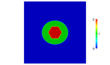
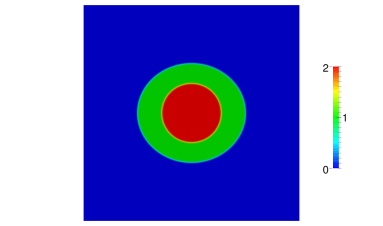
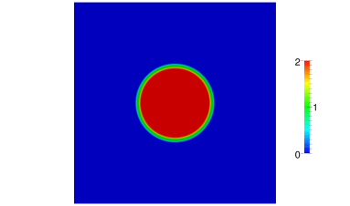
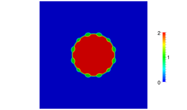
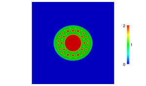
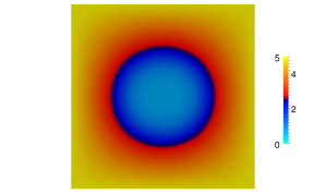
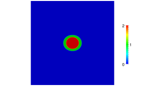
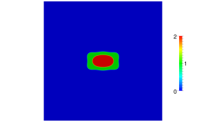
In addition, we set and . For the graphical representation of we will always plot the scalar quantity , which clearly takes on the values in the host, proliferating and necrotic phases, respectively.
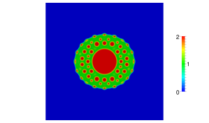
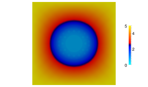
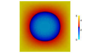
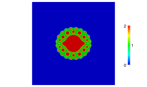
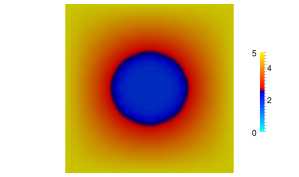
In a first simulation, we investigate the radial growth of the tumour phases for the source term (4.4d) given sufficient nutrient. To this end, we let and
For the values and we start with the perturbed initial profiles defined by (4.10a) and (4.10b), respectively, and observe that in each case the initial perturbations get smoothed out, leading to a nearly radial growth. We show the corresponding simulations in Figures 1 and 2.


In order to investigate the radial growth in more detail, and to study the dependence on the presence of the fluid flow and on the strength of the nutrient source, we repeat the simulations in Figures 1 and 2 for circular initial data, and for different values of and . In particular, we choose in (4.7) and let , with or . Plots of the radii of the two interfacial layers over time for the different parameters can be seen in Figure 3.
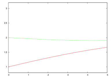
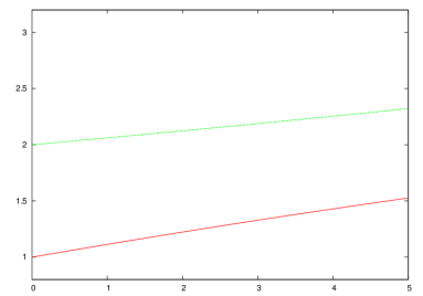
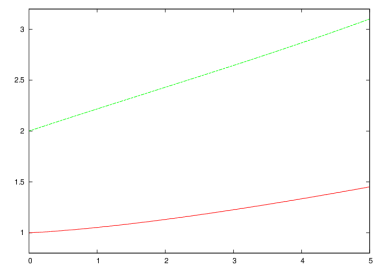
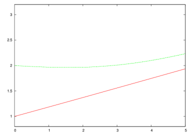
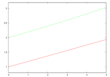
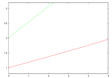
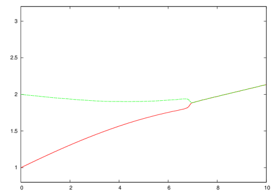
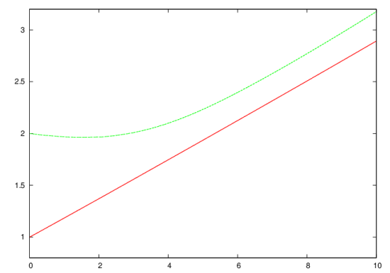
Looking at the results for in particular, we also investigate whether the two radii eventually meet. To this end, we repeat the simulations for a longer time. As observed in Figure 4, in the absence of Darcy flow the inner radius indeed catches up with the outer radius. When Darcy flow is present, however, a constant minimum distance between the two radii is maintained throughout the evolution.
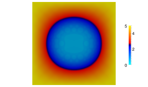
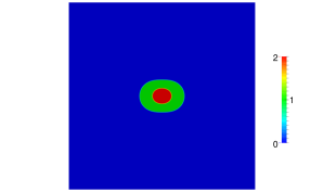
We show some snapshots of the two different evolutions in Figure 5.


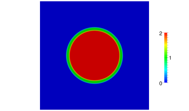
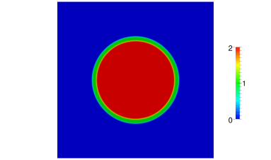
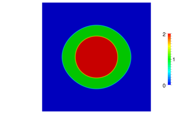
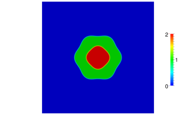
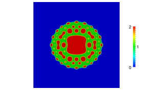
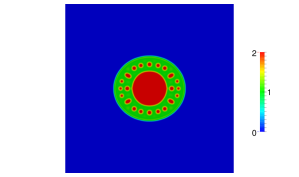
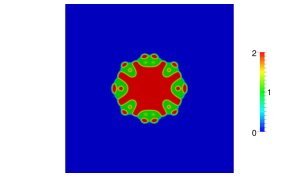
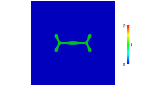
The same simulation as in Figure 1, but now for the source term (4.4b) can be seen in Figure 6. As a comparison we also show the evolution without the fluid flow, see Figure 7. In this case we observe quite complex nucleation phenomena of the necrotic phase within the proliferating phase.


Finally, we consider a numerical simulation on the larger domain for the source term (4.4b), with the parameters
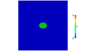
The evolution of the three phases is shown in Figure 8, where we chose the initial radius . It can be seen that both tumour phases grow, with some instabilities developing at the tumour/host cell interface. However, if the initial necrotic phase is smaller, it vanishes and the perturbations become more pronounced, see Figure 9. In fact, towards the end the evolution in Figure 9 becomes similar to [23, Fig. 5].


Let us also point out that the numerical simulations with the source term (4.4c) are almost identical to Figures 8 and 9, and so we omit the results.
We also investigate the effects of a larger initial necrotic core on the evolution of the tumour. To this end, we repeat the computation in Figure 8 for the initial radius for . The three different evolutions can be seen in Figure 10, where we observe that for positive values of , the necrotic core slowly disappears, and the subsequent evolution of the tumour is similar to that observed in Figure 9. Meanwhile, in the case where the necrotic core does not degrade, upon comparing to Figure 8, we can conclude that a large necrotic core seems to suppress or delay the development of protrusions and leads to a more compact growth.


Acknowledgments
The authors gratefully acknowledge the support of the Regensburger Universitätsstiftung Hans Vielberth.
References
- [1] H. Abels, H. Garcke, and G. Grün. Thermodynamically consistent, frame indifferent diffuse interface models for incompressible two-phase flow with different densities. Math. Models Methods Appl. Sci., 22(3):1150013 (40 pages), 2012.
- [2] D. Ambrosi and L. Preziosi. On the closure of mass balance models for tumor growth. Math. Models Methods Appl. Sci., 12(5):737–754, 2002.
- [3] J. W. Barrett, J. F. Blowey, and H. Garcke. On fully practical finite element approximations of degenerate Cahn–Hilliard systems. M2AN Math. Model. Numer. Anal., 35(4):713–748, 2001.
- [4] D. A. Beysens, G. Forgacs, and J. A. Glazier. Cell sorting is analogous to phase ordering in fluids. Proc. Nat. Acad. Sci. USA, 97(17):9467–9471, 2000.
- [5] L. Blank, M. H. Farshbaf-Shaker, H. Garcke, and V. Styles. Relating phase field and sharp interface approaches to structural topology optimization. ESAIM: Control Optim. Calc. Var., 20(4), 2014.
- [6] L. Bronsard, H. Garcke, and B. Stoth. A multi-phase Mullins–Sekerka system: matched asymptotic expansions and an implicit time discretisation for the geometric evolution problem. Proc. Roy. Soc. Edinburgh Sect. A, 128(3):481–506, 1998.
- [7] H. Byrne and L. Preziosi. Modelling solid tumour growth using the theory of mixtures. Math. Med. Biol., 20(4):341–366, 2003.
- [8] Y. Chen and J. S. Lowengrub. Tumor growth in complex, evolving microenvironmental geometries: A diffuse domain approach. J. Theor. Biol., 361:14–30, 2014.
- [9] Y. Chen, S. M. Wise, V. B. Shenoy, and J. S. Lowengrub. A stable scheme for a nonlinear, multiphase tumor growth model with an elastic membrane. Int. J. Numer. Meth. Biomed. Engng., 30:726–754, 2014.
- [10] V. Cristini, X. Li, J. S. Lowengrub, and S. M. Wise. Nonlinear simulations of solid tumor growth using a mixture model: invasion and branching. J. Math. Biol., 58:723–763, 2009.
- [11] V. Cristini and J. Lowengrub. Multiscale modeling of Cancer. Cambridge University Press, 2010.
- [12] V. Cristini, J. Lowengrub, and Q. Nie. Nonlinear simulations of tumor growth. J. Math. Biol., 46:191–224, 2003.
- [13] S. Cui and A. Friedman. Analysis of a mathematical model of the growth of necrotic tumors. J. Math. Anal. Appl., 255(2):636–677, 2001.
- [14] P. Cumsille, A. Coronel, C. Conca, C. Quiñinao, and C. Escudero. Proposal of a hybrid approach for tumor progression and tumor-induced angiogenesis. Theor. Biol. Med. Model., 12(1):13, 2015.
- [15] M. Dai, E. Feireisl, E. Rocca, G. Schimperna, and M. Schonbek. Analysis of a diffuse interface model for multispecies tumor growth. Preprint arXiv:1507.07683, 2015.
- [16] T. A. Davis. Algorithm 832: UMFPACK V4.3—an unsymmetric-pattern multifrontal method. ACM Trans. Math. Software, 30(2):196–199, 2004.
- [17] C. M. Elliott and H. Garcke. Diffusional phase transitions in multicomponent systems with a concentration dependent mobility matrix. Phys. D, 109:242–256, 1997.
- [18] J. Escher, A.-V. Matioc, and B.-V. Matioc. Analysis of a mathematical model describing necrotic tumor growth. In E. Stephan and P. Weiggers, editors, Modelling, simulation and software concepts for scientific-technological problems, volume 57 of Lecture notes in applied and computational mechanics, pages 237–250. Springer Berlin Heidelberg, 2011.
- [19] R. A. Foty, G. Forgacs, C. M. Pfleger, and M. S. Steinberg. Liquid properties of embryonic tissues: Measurement of interfacial tensions. Phys. Rev. Lett., 72:2298–2301, 1994.
- [20] H. B. Frieboes, F. Jin, Y.-L. Chuang, S. M. Wise, J. S. Lowengrub, and V. Cristini. Three-dimensional multispecies nonlinear tumor growth – II: Tumor invasion and angiogenesis. J. Theoret. Biol., 264(4):1254–1278, 2010.
- [21] H. Garcke and R. Haas. Modelling of non-isothermal multi-component, multi-phase systems with convection. In D. M. Herlach, editor, Phase Transformations in Multicomponent Melts, pages 325–338. Wiley-VCH Verlag, Weinheim, 2008.
- [22] H. Garcke and K. F. Lam. Global weak solutions and asymptotic limits of a Cahn–Hilliard–Darcy system modelling tumour growth. AIMS Mathematics, 1(3):318–360, 2016.
- [23] H. Garcke, K. F. Lam, E. Sitka, and V. Styles. A Cahn–Hilliard–Darcy model for tumour growth with chemotaxis and active transport. Math. Models Methods Appl. Sci., 26(6):1095–1148, 2016.
- [24] H. Garcke, B. Nestler, and B. Stinner. A diffuse interface model for alloys with multiple components and phases. SIAM J. Appl. Math, 64(3):775–799, 2004.
- [25] H. Garcke, B. Nestler, and B. Stoth. On anisotropic order parameter models for multi-phase systems and their sharp interface limits. Phys. D, 115(1):87–108, 1998.
- [26] H. Garcke, B. Nestler, and B. Stoth. A multiphase field concept: numerical simulations of moving phase boundaries and multiple junctions. SIAM J. Appl. Math., 60(1):295–315, 1999.
- [27] H. Garcke and B. Stinner. Second order phase field asymptotics for multi-component systems. Interfaces Free Bound., 8:131–157, 2006.
- [28] M. E. Gurtin. On a nonequilibrium thermodynamics of capillarity and phase. Quart. Appl. Math., 47(1):129–145, 1989.
- [29] M. E. Gurtin. Generalized Ginzburg–Landau and Cahn–Hilliard equations based on a microforce balance. Phys. D, 92(3-4):178–192, 1996.
- [30] M. E. Gurtin, E. Fried, and L. Anand. The mechanics and thermodynamics of continua. Cambridge University Press, 2010.
- [31] A. Hawkins-Daarud, K. G. van der Zee, and J. T. Oden. Numerical simulation of a thermodynamically consistent four-species tumor growth model. Int. J. Numer. Method Biomed. Eng., 28(1):3–24, 2012.
- [32] D. Hilhorst, J. Kampmann, T. N. Nguyen, and K. G. van der Zee. Formal asymptotic limit of a diffuse-interface tumor-growth model. Math. Models Methods Appl. Sci., 25(6):1011–1043, 2015.
- [33] T. Hillen and K. J. Painter. A user’s guide to PDE models for chemotaxis. J. Math. Biol., 58(1-2):183–217, 2009.
- [34] D. Horstmann. From 1970 until present: the Keller–Segel model in chemotaxis and its consequences. I. Jahresberichte DMV, 105(3):103–165, 2003.
- [35] E. F. Keller and L. A. Segel. Initiation of slime mold aggregation viewed as an instability. J. Theoret. Biol., 26(3):399–415, 1970.
- [36] E. F. Keller and L. A. Segel. Model for Chemotaxis. J. Theoret. Biol., 30(2):225–234, 1971.
- [37] E. A. B. F. Lima, R. C. Almeida, and J. T. Oden. Analysis and numerical solution of stochastic phase-field models of tumor growth. Numer. Methods Partial Differential Equations, 31(2):552–574, 2015.
- [38] E. A. B. F. Lima, J. T. Odent, and R. C. Almeida. A hybrid ten-species phase-field model of tumor growth. Math. Models Methods Appl. Sci., 24(13):2569–2599, 2014.
- [39] I.-S. Liu. Continuum mechanics. Advanced Texts in Physics. Springer–Verlag, Berlin, 2002.
- [40] P. Macklin and J. Lowengrub. An improved geometry-aware curvature discretization for level set methods: Application to tumor growth. J. Sci. Comput., 215:392–401, 2006.
- [41] P. Macklin and J. Lowengrub. Nonlinear simulation of the effect of microenvironment on tumor growth. J. Theoret. Biol., 245:677–704, 2007.
- [42] P. Macklin and J. S. Lowengrub. A new ghost cell/level set method for moving boundary problems: Application to tumor growth. J. Sci. Comput., 35(2-3):266–299, 2008.
- [43] A. Novick-Cohen. Triple-junction motion for an Allen–Cahn/Cahn–Hilliard system. Phys. D, 137(1–2):1–24, 2000.
- [44] R. Nürnberg. Numerical simulations of immiscible fluid clusters. Appl. Numer. Math., 59:1612–1628, 2009.
- [45] J. T. Oden, A. Hawkins, and S. Prudhomme. General diffuse-interface theories and an approach to predictive tumor growth modeling. Math. Models Methods Appl. Sci., 20(3):477–517, 2010.
- [46] S. Pennacchietti, P. Michieli, M. Galluzzo, M. Mazzone, S. Giordano, and P. M. Comoglio. Hypoxia promotes invasive growth by transcriptional activation of the met protooncogene. Cancer Cell, 3:347–361, 2003.
- [47] K. Pham, H. B. Frieboes, V. Cristini, and J. Lowengrub. Predictions of tumour morphological stability and evaluation against experimental observations. J. R. Soc. Interface, 8:16–29, 2011.
- [48] P. Podio-Guidugli. Models of phase segregation and diffusion of atomic species on a lattice. Ric. Mat., 55(1):105–118, 2006.
- [49] L. Preziosi and A. Tosin. Multiphase modelling of tumour growth and extracellular matrix interaction: mathematical tools and applications. J. Math. Biol., 58:625–656, 2009.
- [50] J. Ranft, M. Basan, J. Elgeti, J.-F. Joanny, J. Prost, and F. Jülicher. Fluidization of tissues by cell division and apoptosis. Proc. Nat. Acad. Sci. USA, 107(49):20863–20868, 2010.
- [51] S. Rey and G. L. Semenza. Hypoxia-inducible factor-1-dependent mechanisms of vascularization and vascular remodelling. Cardiovasc Res., 86(2):236–242, 2010.
- [52] A. Schmidt and K. G. Siebert. Design of Adaptive Finite Element Software: The Finite Element Toolbox ALBERTA, volume 42 of Lecture Notes in Computational Science and Engineering. Springer-Verlag, Berlin, 2005.
- [53] P. Sternberg. Vector-valued local minimizers of nonconvex variational problems. Rocky Mountain J. Math., 21:799–807, 1991.
- [54] S. M. Wise, J. S. Lowengrub, H. B. Frieboes, and V. Cristini. Three-dimensional multispecies nonlinear tumor growth - I: Model and numerical method. J. Theoret. Biol., 253(3):524–543, 2008.
- [55] J. Xu, G. Vilanova, and H. Gomez. A mathematical model coupling tumor growth and angiogenesis. PLoS ONE, 11(2):e0149422, 2016.
- [56] H. Youssefpour, X. Li, A. D. Lander, and J. S. Lowengrub. Multispecies model of cell lineages and feedback control in solid tumors. J. Theoret. Biol., 304:39–59, 2012.
- [57] X. Zheng, S. M. Wise, and V. Cristini. Nonlinear simulation of tumor necrosis, neo-vascularization and tissue invasion via an adaptive finite-element/level-set method. Bull. Math. Biol., pages 211–259, 2005.