Fast evaluation of solid harmonic Gaussian integrals for local resolution-
of-the-identity methods and range-separated hybrid functionals

Abstract

An integral scheme for the efficient evaluation of two-center integrals over contracted solid harmonic Gaussian functions is presented. Integral expressions are derived for local operators that depend on the position vector of one of the two Gaussian centers. These expressions are then used to derive the formula for three-index overlap integrals where two of the three Gaussians are located at the same center. The efficient evaluation of the latter is essential for local resolution-of-the-identity techniques that employ an overlap metric. We compare the performance of our integral scheme to the widely used Cartesian Gaussian-based method of Obara and Saika (OS). Non-local interaction potentials such as standard Coulomb, modified Coulomb and Gaussian-type operators, that occur in range-separated hybrid functionals, are also included in the performance tests. The speed-up with respect to the OS scheme is up to three orders of magnitude for both, integrals and their derivatives. In particular, our method is increasingly efficient for large angular momenta and highly contracted basis sets.

I Introduction

The rapid analytic evaluation of two-center Gaussian integrals is important for many molecular simulation methods. For example, Gaussian functions are widely used as orbital basis in quantum mechanical (QM) calculations and are implemented in many electronic-structure codes.Ahlrichs et al. (1989); Hutter et al. (2014); dal ; Werner et al. (2012); Schmidt et al. (1993); Frisch et al. Gaussians are further used at lower level of theory to model charge distributions in molecular mechanicsPiquemal et al. (2006); Cisneros, Piquemal, and Darden (2006); Elking, Darden, and Woods (2007); Gresh et al. (2007); Elking et al. (2010); Cisneros (2012); Simmonett et al. (2014); Chaudret et al. (2014); Giese et al. (2015) (MM), semi-empiricalKoskinen and Mäkinen (2009); Bernstein, Mehl, and Papaconstantopoulos (2002); Giese and York (2005) and hybrid QM/MM methods.Giese and York (2007); Golze et al. (2013); Giese and York (2016a) The Gaussian-based treatment of the electrostatic interactions requires the evaluation of two-center Coulomb integrals.

The efficient evaluation of two-center integrals is also important at the Kohn-Sham density functional theory (KS-DFT) level, in particular for hybrid density functionals. In order to speed-up the evaluation of the Hartree-Fock exchange term, the exact evaluation of the four-center integrals can be replaced by resolution-of-the-identity (RI) approximations.Sodt and Head-Gordon (2008); Manzer, Epifanovsky, and Head-Gordon (2015); Ihrig et al. (2015); Levchenko et al. (2015) Especially, when an overlap metric is employed, the efficient evaluation of two-center integrals is required. The interaction potential can take different functional forms dependent on the hybrid functionals.Guidon et al. (2008) The most popular potential is the standard Coulomb operator employed in well-established functionals such as PBE0Perdew, Burke, and Ernzerhof (1996); Ernzerhof, Perdew, and Burke (1997); Ernzerhof and Scuseria (1999) and B3LYP.Becke (1993); Lee, Yang, and Parr (1988); Vosko, Wilk, and Nusair (1980) A short-range Coulomb potential is, e.g., employed for the HSE06 functional,Heyd, Scuseria, and Ernzerhof (2003, 2006); Krukau et al. (2006) whereas a combination of long-range Coulomb and Gaussian-type potential is used for the MCY3 functional.Cohen, Mori-Sánchez, and Yang (2007)

Gaussian overlap integrals, in the following denoted by $(ab)$, are computed in semi-empirical methodsKoskinen and Mäkinen (2009) and QM approaches such as Hartree-Fock and KS-DFT. The efficient computation of $(ab)$ is not of major importance for QM methods since their contribution to the total computational cost is negligible. However, the efficient evaluation of the three-index overlap integrals $(ab\tilde{a})$, where two functions are located at the same center, is essential for local RI approaches that use an overlap metric.Baerends, Ellis, and Ros (1973); Guerra et al. (1998); te Velde et al. (2001) Employing local RI in KS-DFT, the atomic pair densities are approximated by an expansion in atom-centered auxiliary functions. In order to solve the RI equations, it is necessary to calculate $(ab\tilde{a})$ for each pair where $a,b$ refers to orbital functions at atoms A and B and $\tilde{a}$ to the auxiliary function at A. The evaluation of $(ab\tilde{a})$ is computationally expensive because the auxiliary basis set is 3-5 times larger than the orbital basis set. A rapid evaluation of $(ab\tilde{a})$ is important to ensure that the computational overhead of the integral calculation is not larger than the speed-up gained by the RI .

Two-center integrals with the local operator $r_{a}^{2n}$ ($n\in\mathbb{N}$), where $r_{a}$ depends on the center of one of the Gaussian functions, are required for special projection and expansion techniques. For example, these integrals are used for projection of the primary orbital basis on smaller, adaptive basis sets.Schütt and VandeVondele (2016)

Numerous schemes for the evaluation of Gaussian integrals have been proposed based on Cartesian Gaussian,Dupuis, Rys, and King (1976); Obara and Saika (1986); Head-Gordon and Pople (1988); Lindh, Ryu, and Liu (1991); Bracken and Bartlett (1997); Gill, Gilbert, and Adams (2000); Ahlrichs (2006) Hermite Gaussian McMurchie and Davidson (1978); Helgaker and Taylor (1992); Klopper and Röhse (1992); Reine, Tellgren, and Helgaker (2007) and solid or spherical harmonic Gaussian functions.Dunlap (1990, 2001, 2003); Hu and Dunlap. (2013); Reine, Tellgren, and Helgaker (2007); Giese and York (2008); Kuang and Lin (1997a, b) For a review of Gaussian integral schemes see Ref. Reine, Helgaker, and Lindh, 2012. A very popular approach is the Obara-Saika (OS) scheme,Obara and Saika (1986) which employs a recursive formalism over primitive Cartesian Gaussian functions. However, electronic-structure codes utilize spherical harmonic Gaussians (SpHGs) since the number of SpHGs is equal or smaller than the number of Cartesian Gaussians, i.e. for fixed angular momentum $l$, $(2l+1)$ SpHGs compare to $(l+1)(l+2)/2$ Cartesian Gaussians. Furthermore, Gaussian basis sets are often constituted of contracted functions. Thus, the primitive Cartesian integrals obtained from the OS recursion are subsequently contracted and transformed to SpHGs.

In this work, we further develop an alternative integral schemeDunlap (1990, 2001, 2003); Giese and York (2008) that employs contracted solid harmonic Gaussians (SHGs). The latter are closely related to SpHG functions and differ solely by a constant factor. The SHG integral scheme is based on the application of the spherical tensor gradient operator (STGO).Weniger and Steinborn (1985); Weniger (2005) The expressions resulting from Hobson’s theorem of differentiationHobson (1892) contain an angular momentum term that is independent on the exponents and contraction coefficients. This term is obtained by relatively simple recursions. It can be pre-computed and re-used multiple times for all functions in the basis set with the same $l$ and $m$ quantum number. The integral and derivative evaluation requires the contraction of a set of auxiliary integrals over $s$ functions and their scalar derivatives. The same contracted quantity is re-used several times for the evaluation of functions with the same set of exponents and contraction coefficients, but different angular dependency $m$. Unlike for Cartesian functions, subsequent transformation and contraction steps are not required.

This work is based on Refs. Giese and York, 2008, 2016b, where the two-index integral expressions for the overlap operator and general non-local operators are given. We extend the SHG scheme to the local operator $r_{a}^{2n}$ and derive formulas for the integrals $(a|r_{a}^{2n}|b)$. The latter are fundamental for the subsequent derivation of the three-index overlap integral $(ab\tilde{a})$. The performance of the SHG method is compared to the OS scheme. We also include integrals with different non-local operators such as standard Coulomb, modified Coulomb or Gaussian-type operators in our comparison.

In the next section, the expressions for the integrals and their Cartesian derivatives are given followed by details on the implementation of the integral schemes. The performance of the SHG scheme is then discussed in terms of number of operations and empirical timings. The derivations of the expressions for $(a|r_{a}^{2n}|b)$ are given in Appendix A and B.

II Integral and derivative evaluation

After introducing the relevant definitions and notations, we summarize the work of Giese and YorkGiese and York (2008) in Section II.2. The integral expressions of $(a|r_{a}^{2n}|b)$ and $(ab\tilde{a})$ are then derived in Sections II.3 and II.4, respectively. Subsequently, the formulas for the Cartesian derivatives are given (Section II.5) as well as the details on the computation of the angular-dependent term in the SHG integral expressions (Section II.6).

II.1 Definitions and notations

The notations used herein correspond to Refs. Watson et al., 2004; Helgaker, Jørgensen, and Olsen, 2012; Giese and York, 2008 unless otherwise indicated. An unnormalized, primitive SHG function is defined as

$$\chi_{l,m}(\alpha,\mathbf{r})=C_{l,m}(\mathbf{r})\exp{(-\alpha r^{2})}$$ (1)

where the complex solid harmonics $C_{l,m}(\mathbf{r})$,

$$C_{l,m}(\mathbf{r})=\sqrt{\frac{4\pi}{2l+1}}r^{l}Y_{l,m}(\theta,\phi),$$ (2)

are obtained by rescaling the spherical harmonics $Y_{l,m}(\theta,\phi)$. Contracted SpHG functions $\varphi_{l,m}(\mathbf{r})$ are constructed as linear combination of the primitive SHG functions

$$\varphi_{l,m}(\mathbf{r})=N_{l}\sum_{\alpha\in A}c_{\alpha}\chi_{l,m}(\alpha,\mathbf{r}),$$ (3)

where $\{c_{\alpha}\}$ are the contraction coefficients for the set of exponents $A=\{\alpha\}$ and $N_{l}$ is the normalization constant given bySchlegel and Frisch (1995)

$$N_{l}=K_{l}\left[\sum_{\alpha\in A}\sum_{\hat{\alpha}\in A}\frac{\pi^{1/2}(2l+2)!c_{\alpha}c_{\hat{\alpha}}}{2^{2l+3}(l+1)!(\alpha+\hat{\alpha})^{l+3/2}}\right]^{-1/2}.$$ (4)

The factor

$$K_{l}=\sqrt{\frac{2l+1}{4\pi}}$$ (5)

is included in the normalization constant to convert from SHG to SpHG functions.

In the following, the absolute value of the $m$ quantum number is denoted by

$$\mu=|m|.$$ (6)

Furthermore, we use the notations,

$$\mathbf{r}_{a}=\mathbf{r}-\mathbf{R}_{a},\quad\mathbf{r}_{b}=\mathbf{r}-\mathbf{R}_{b},\quad R_{ab}^{2}=|\mathbf{R}_{a}-\mathbf{R}_{b}|^{2},$$ (7)

where $\mathbf{R}_{a}$ references the position of the Gaussian center A and $\mathbf{R}_{b}$ the position of center B. The scalar derivative of $X(r^{2})$ with respect to $r^{2}$ is denoted by

$$X^{(k)}(r^{2})=\left(\frac{\partial}{\partial r^{2}}\right)^{k}X(r^{2}).$$ (8)

II.2 Integrals $(a|\mathcal{O}|b)$

In this section, the expression to compute the two-center integral $(a|\mathcal{O}|b)$ is given which is defined as

$$\begin{split}(a|\mathcal{O}|b)=\iint&\varphi_{l_{a},m_{a}}(\mathbf{r}_{1}-\mathbf{R}_{a})\mathcal{O}(\mathbf{r}_{1}-\mathbf{r}_{2})\\ &\times\varphi_{l_{b},m_{b}}(\mathbf{r}_{2}-\mathbf{R}_{b})d\mathbf{r}_{1}d\mathbf{r}_{2}.\end{split}$$ (9)

$\varphi_{l_{a},m_{a}}(\mathbf{r}_{a})$ and $\varphi_{l_{b},m_{b}}(\mathbf{r}_{b})$ are contracted SpHG functions as defined in Equation (3), which are centered at $\mathbf{R}_{a}$ and $\mathbf{R}_{b}$, respectively. $\mathcal{O}(\mathbf{r})$ is an operator that is explicitly independent on the position vectors $\mathbf{R}_{a}$ or $\mathbf{R}_{b}$. Such operators are, e.g., the non-local Coulomb operator $\mathcal{O}(\mathbf{r})=1/r$ or the local overlap $\mathcal{O}(\mathbf{r})=\delta(\mathbf{r})$.

The derivation for an efficient expression to compute $(a|\mathcal{O}|b)$ follows Ref. Giese and York, 2008. It is based on Hobson’s theoremHobson (1892) of differentiation, which states that

$$C_{l,m}(\nabla)f(r^{2})=2^{l}C_{l,m}(\mathbf{r})\left(\frac{\partial}{\partial r^{2}}\right)^{l}f(r^{2}),$$ (10)

where the differential operator $C_{l,m}(\nabla)$ is called STGO. The differential operator is obtained by replacing $\mathbf{r}$ in the solid harmonic $C_{l,m}(\mathbf{r})$ by $\nabla=(\partial/\partial x,\partial/\partial y,\partial/\partial z)$. The derivation of the $(a|\mathcal{O}|b)$ integrals starts by noting that $\exp(-\alpha r^{2})$ is an eigenfunction of $(\displaystyle{\partial/\partial r^{2}})^{l}$ with the eigenvalue $(-\alpha)^{l}$. Using Equation (10) and the definition of primitive SHGs from Equation (1), the primitive SHG at center $\mathbf{R}_{a}$ can be rewritten as

$$\chi_{l,m}(\alpha,\mathbf{r}_{a})=\frac{C_{l,m}(\nabla_{a})\exp{\left(-\alpha r_{a}^{2}\right)}}{(2\alpha)^{l}},$$ (11)

where $C_{l,m}(\nabla_{a})$ acts on $\mathbf{R}_{a}$. Inserting Equation (1) for $s$ functions, $\chi_{0,0}(\alpha,\mathbf{r})=\exp{\left(-\alpha r^{2}\right)}$, yields

$$\chi_{l,m}(\alpha,\mathbf{r}_{a})=\frac{C_{l,m}(\nabla_{a})\chi_{0,0}(\alpha,\mathbf{r}_{a})}{(2\alpha)^{l}}.$$ (12)

Inserting the STGO formulation of $\chi_{l,m}$ from Equation (12) in Equation (9) gives

$$(a|\mathcal{O}|b)=C_{l_{a},m_{a}}(\nabla_{a})C_{l_{b},m_{b}}(\nabla_{b})O_{l_{a},l_{b}}(R_{ab}^{2}).$$ (13)

The contracted integral over $s$ functions is denoted by

$$O_{l_{a},l_{b}}(R_{ab}^{2})=N_{l_{a}}N_{l_{b}}\sum_{\alpha\in A}\sum_{\beta\in B}\frac{c_{\alpha}c_{\beta}}{(2\alpha)^{l_{a}}(2\beta)^{l_{b}}}(0_{a}|\mathcal{O}|0_{b}),$$ (14)

where $c_{\alpha}$ and $c_{\beta}$ are the expansion coefficients of $\varphi_{l_{a},m_{a}}(\mathbf{r}_{a})$ and $\varphi_{l_{b},m_{b}}(\mathbf{r}_{b})$, respectively, with corresponding exponents $\alpha$ and $\beta$. The integral $(0_{a}|\mathcal{O}|0_{b})$ over primitive $s$ functions is given by

$$\begin{split}(0_{a}|\mathcal{O}|0_{b})=\iint&\chi_{0,0}(\alpha,\mathbf{r}_{1}-\mathbf{R}_{a})\mathcal{O}(\mathbf{r}_{1}-\mathbf{r}_{2})\\ &\times\chi_{0,0}(\beta,\mathbf{r}_{2}-\mathbf{R}_{b})d\mathbf{r}_{1}d\mathbf{r}_{2}.\end{split}$$ (15)

The analytic expressions of $(0_{a}|\mathcal{O}|0_{b})$ for the overlap and different non-local operators are given in Table S1, see Supplementary Information (SI). Application of the product and differentiation rules for the STGOHu et al. (2000); Dunlap (1990, 2001, 2003) finally yields

$$\begin{split}(a|\mathcal{O}|b)=&(-1)^{l_{b}}A_{l_{a},m_{a}}A_{l_{b},m_{b}}\\[5.0pt] &\times\sum_{j=0}^{\mathrm{min}(l_{a},l_{b})}2^{l_{a}+l_{b}-j}O^{(l_{a}+l_{b}-j)}_{l_{a},l_{b}}(R_{ab}^{2})\\ &\times(2j-1)!!\sum_{\kappa=0}^{j}B_{j,\kappa}Q_{l_{a},\mu_{a},l_{b},\mu_{b},j,\kappa}^{c/s,c/s}(\mathbf{R}_{ab}),\end{split}$$ (16)

where the prefactors are

$$A_{l,m} =(-1)^{m}\sqrt{(2-\delta_{m,0})(l+m)!(l-m)!}$$ (17)

$$B_{j,\kappa} =\frac{1}{(2-\delta_{\kappa,0})(j+\kappa)!(j-\kappa)!}\,.$$ (18)

and $n!!$ denotes the double factorial. The superscript on $O_{l_{a},l_{b}}(R_{ab}^{2})$ in Equation (16) denotes the scalar derivative with respect to $R_{ab}^{2}$, see Equation (8) and (14),

$$\begin{split}O^{(k)}_{l_{a},l_{b}}(R_{ab}^{2})=&N_{l_{a}}N_{l_{b}}\sum_{\alpha\in A}\sum_{\beta\in B}\frac{c_{\alpha}c_{\beta}}{(2\alpha)^{l_{a}}(2\beta)^{l_{b}}}\\ &\times\left(\frac{\partial}{\partial R_{ab}^{2}}\right)^{k}(0_{a}|\mathcal{O}|0_{b}).\end{split}$$ (19)

Since $s$ functions contain no angular dependency, $(0_{a}|\mathcal{O}|0_{b})$ is a function of $\mathbf{R}_{ab}$ (or equivalently, $R_{ab}^{2}$), see Table S1 (SI). Therefore, the derivative in Equation (19) is well-defined. The integral $O_{l_{a},l_{b}}(R_{ab}^{2})$ can be interpreted as the monopole result of the expansion given in Equation (16).

The expression given in Equation (16) depends further on $Q_{l_{a},\mu_{a},l_{b},\mu_{b},j,\kappa}^{c/s,c/s}(\mathbf{R}_{ab})$, where $\mu=|m|$. Positive $m$ values refer to a cosine ($c$) component and negative $m$ to a sine ($s$) component, i.e.

$$\begin{split}Q_{a,b,j,\kappa}^{cc}(\mathbf{R}_{ab}):&\hskip 10.00002ptm_{a},m_{b}\geq 0\\ Q_{a,b,j,\kappa}^{cs}(\mathbf{R}_{ab}):&\hskip 10.00002ptm_{a}\geq 0,m_{b}<0\\ Q_{a,b,j,\kappa}^{sc}(\mathbf{R}_{ab}):&\hskip 10.00002ptm_{a}<0,m_{b}\geq 0\\ Q_{a,b,j,\kappa}^{ss}(\mathbf{R}_{ab}):&\hskip 10.00002ptm_{a},m_{b}<0\,.\end{split}$$ (20)

Note that we used the abbreviation $a,b$ for the indices $(l_{a},\mu_{a},l_{b},\mu_{b})$ in Equation (20). Details on the calculation of $Q_{a,b,j,\kappa}^{c/s,c/s}(\mathbf{R}_{ab})$ can be found in Section II.6.

II.3 Integrals $(a|r_{a}^{2n}|b)$

The integrals $(a|r_{a}^{2n}|b)$,

$$(a|r_{a}^{2n}|b)=\int\varphi_{l_{a},m_{a}}(\mathbf{r}_{a})r_{a}^{2n}\varphi_{l_{b},m_{b}}(\mathbf{r}_{b})d\mathbf{r}\,,$$ (21)

$n\in\mathbb{N}$, are fundamental for the derivation of the overlap matrix elements $(ab\tilde{a})$ with two Gaussians at center $\mathbf{R}_{a}$, which are discussed in the next section. Since the operator $r_{a}^{2n}$ depends on the position $\mathbf{R}_{a}$, Equations (14) and (16) cannot be adapted by replacing $(0_{a}|\mathcal{O}|0_{b})$ with $(0_{a}|r_{a}^{2n}|0_{b})$. Consequently, new expressions for computing $(a|r_{a}^{2n}|b)$ are derived in this section.

Since $r_{a}^{2n}$ depends on $\mathbf{R}_{a}$, $C_{l,m}(\nabla_{a})$ is acting on the product of $\chi_{l,m}(\alpha,\mathbf{r}_{a})$ and $r_{a}^{2n}$,

$$\chi_{l,m}(\alpha,\mathbf{r}_{a})r_{a}^{2n}=C_{l,m}(\mathbf{r}_{a})\exp{\left(-\alpha r_{a}^{2}\right)}r_{a}^{2n}.$$ (22)

The expression of this product in terms of the STGO $C_{l,m}(\nabla_{a})$ is obtained using Hobson’s theorem,

$$\begin{split}\chi_{l,m}(\alpha,\mathbf{r}_{a})r_{a}^{2n}=\frac{C_{l,m}(\nabla_{a})}{(2\alpha)^{l}}\sum_{j=0}^{n}&\binom{n}{j}\frac{(l+j-1)!}{(l-1)!\alpha^{j}}\\ &\times\exp{\left(-\alpha r_{a}^{2}\right)}r_{a}^{2(n-j)}.\end{split}$$ (23)

The derivation of Equation (23) is given in Appendix A.

Inserting Equations (12) and (23) in Equation (21) yields

$$(a|r_{a}^{2n}|b)=C_{l_{a},m_{a}}(\nabla_{a})C_{l_{b},m_{b}}(\nabla_{b})T_{l_{a},l_{b}}(R_{ab}^{2}),$$ (24)

where $T_{l_{a},l_{b}}(R_{ab}^{2})=T_{l_{a},l_{b}}^{(0)}(R_{ab}^{2})$ is again the monopole results for the integral given in Equation (25). The derivation follows now the same procedure as for the integrals $(a|\mathcal{O}|b)$ and yields

$$\begin{split}(a|r_{a}^{2n}|b)=&(-1)^{l_{b}}A_{l_{a},m_{a}}A_{l_{b},m_{b}}\\[5.0pt] &\times\sum_{j=0}^{\mathrm{min}(l_{a},l_{b})}2^{l_{a}+l_{b}-j}T^{(l_{a}+l_{b}-j)}_{l_{a},l_{b}}(R_{ab}^{2})\\ &\times(2j-1)!!\sum_{\kappa=0}^{j}B_{j,\kappa}Q_{l_{a},\mu_{a},l_{b},\mu_{b},j,\kappa}^{c/s,c/s}(\mathbf{R}_{ab}),\end{split}$$ (25)

where the scalar derivative of $T_{l_{a},l_{b}}(R_{ab}^{2})$ with respect to $R_{ab}^{2}$ is

$$\begin{split}T^{(k)}_{l_{a},l_{b}}(R_{ab}^{2})=&N_{l_{a}}N_{l_{b}}\sum_{\alpha\in A}\sum_{\beta\in B}\frac{c_{\alpha}c_{\beta}}{(2\alpha)^{l_{a}}(2\beta)^{l_{b}}}\\ &\times\sum_{j=0}^{n}\binom{n}{j}\frac{(l_{a}+j-1)!}{(l_{a}-1)!\alpha^{j}}(0_{a}|r_{a}^{2(n-j)}|0_{b})^{(k)}.\end{split}$$ (26)

The integral over primitive $s$ functions is

$$(0_{a}|r_{a}^{2m}|0_{b}) =\int\chi_{0,0}(\alpha,\mathbf{r}_{a})r_{a}^{2m}\chi_{0,0}(\beta,\mathbf{r}_{b})d\mathbf{r}$$ (27)

$$=\frac{\pi^{3/2}\exp(-\rho R_{ab}^{2})}{2^{m}c^{m+3/2}}\sum_{j=0}^{m}I_{j}^{\alpha,\beta,m}(R_{ab}^{2})$$ (28)

with $c=\alpha+\beta$ and $\rho=\alpha\beta/c$ and

$$I_{j}^{\alpha,\beta,m}(R_{ab}^{2})=2^{j}\frac{(2m+1)!!\binom{m}{j}}{(2j+1)!!}\frac{\beta^{2j}}{c^{j}}R_{ab}^{2j}.$$ (29)

The proof of Equation (28) is similarly elaborate as for Equation (23) and is given in Appendix B. The derivatives of $(0_{a}|r_{a}^{2m}|0_{b})$ are obtained by applying the Leibniz rule of differentiation to Equation (28)

$$\begin{split}(0_{a}|&r_{a}^{2m}|0_{b})^{(k)}\\ =&\frac{\pi^{3/2}\exp(-\rho R_{ab}^{2})}{2^{m}c^{m+3/2}}\sum_{i=0}^{\mathrm{min}(m,k)}\binom{k}{i}\left(-\rho\right)^{k-i}\\ &\times\sum_{j=i}^{m}\left(\frac{\partial}{\partial R_{ab}^{2}}\right)^{i}I_{j}^{\alpha,\beta,m}(R_{ab}^{2}).\end{split}$$ (30)

II.4 Overlap integrals $(ab\tilde{a})$

The three-index overlap integral $(ab\tilde{a})$ includes two functions at center $\mathbf{R}_{a}$ and is defined by

$$(ab\tilde{a})=\int\varphi_{l_{a},m_{a}}(\mathbf{r}_{a})\varphi_{\tilde{l}_{a},\tilde{m}_{a}}(\mathbf{r}_{a})\varphi_{l_{b},m_{b}}(\mathbf{r}_{b})d\mathbf{r}.$$ (31)

In traditional Cartesian Gaussian-based schemes, the product of the two Cartesian functions at center $\mathbf{R}_{a}$ is obtained by adding exponents and angular momenta of both Gaussians, respectively. The result is a new Cartesian Gaussian at $\mathbf{R}_{a}$. The integral evaluation proceeds then as for the two-index overlap integrals $(ab)$. In the SHG scheme on the other hand, the product of two SHG functions at the same center is obtained by a Clebsch-Gordan (CG) expansion of the spherical harmonics. In the following, the expression of this expansion in terms of the STGO is derived and used to obtain the integral formula.

Employing the definitions given in Equations (1) and (2), the product of two primitive SHG functions at $\mathbf{R}_{a}$ can be written as

$$\chi_{l,m} (\alpha,\mathbf{r}_{a})\chi_{\tilde{l},\tilde{m}}(\tilde{\alpha},\mathbf{r}_{a})$$

$$=C_{l,m}(\mathbf{r}_{a})\exp(-\alpha r_{a}^{2})C_{\tilde{l},\tilde{m}}(\mathbf{r}_{a})\exp(-\tilde{\alpha}r_{a}^{2})$$ (32)

$$=\lambda\exp\left(-\alpha^{\prime}r_{a}^{2}\right)Y_{l,m}(\theta,\phi)Y_{\tilde{l},\tilde{m}}(\theta,\phi)r_{a}^{l+\tilde{l}}$$ (33)

where $\alpha^{\prime}=\alpha+\tilde{\alpha}$ and

$$\lambda=\frac{4\pi}{\sqrt{(2l+1)(2\tilde{l}+1)}}.$$ (34)

The product of two spherical harmonics can be expanded in terms of spherical harmonics,

$$Y_{l,m}(\theta,\phi)Y_{\tilde{l},\tilde{m}}(\theta,\phi)=\sum_{L,M}G^{L,l,\tilde{l}}_{M,m,\tilde{m}}Y_{L,M}(\theta,\phi),$$ (35)

where $|l-\tilde{l}|\leq L\leq l+\tilde{l}$. $G^{L,l,\tilde{l}}_{M,m,\tilde{m}}$ are the Gaunt coefficientsGaunt (1929) which are proportional to a product of CG coefficients.Xu (1996) The expansion given in Equation (35) is valid since the spherical harmonics form a complete set of orthonormal functions. A similar expansion for solid harmonics $C_{l,m}(\mathbf{r})$ is not possible because the latter are no basis of ${L}^{2}(\mathbb{R}^{3})$. Inserting the CG expansion into Equation (33) [1], re-introducing solid harmonics [2] as defined in Equation (2) and employing the definition given in Equation (1) [3] yields

$$\chi_{l,m} (\alpha,\mathbf{r}_{a})\chi_{\tilde{l},\tilde{m}}(\tilde{\alpha},\mathbf{r}_{a})$$

$$\stackrel{{\scriptstyle[1]}}{{=}}\lambda\exp\left(-\alpha^{\prime}r_{a}^{2}\right)\sum_{L,M}G^{L,l,\tilde{l}}_{M,m,\tilde{m}}Y_{L,M}(\theta,\phi)r_{a}^{l+\tilde{l}}$$ (36)

$$\stackrel{{\scriptstyle[2]}}{{=}}\lambda\sum_{L,M}G^{L,l,\tilde{l}}_{M,m,\tilde{m}}K_{L}C_{L,M}(\mathbf{r}_{a})$$

$$\qquad\qquad\times\exp\left(-\alpha^{\prime}r_{a}^{2}\right)r_{a}^{l+\tilde{l}-L}$$ (37)

$$\stackrel{{\scriptstyle[3]}}{{=}}\lambda\sum_{L,M}G^{L,l,\tilde{l}}_{M,m,\tilde{m}}K_{L}\chi_{L,M}(\alpha^{\prime},\mathbf{r}_{a})r_{a}^{l+\tilde{l}-L},$$ (38)

where $K_{L}$ is defined in Equation (5). The $L$ quantum numbers of the non-vanishing contributions in the CG expansion proceed in steps of two starting from $L_{\mathrm{min}}=|l-\tilde{l}|$ to $L_{\mathrm{max}}=l+\tilde{l}$. Thus, $l+\tilde{l}-L$ is even and we can express $\chi_{L,M}(\alpha^{\prime},\mathbf{r}_{a})r_{a}^{l+\tilde{l}-L}$ in terms of the STGO using Equation (23),

$$\begin{split}\chi_{l,m}&(\alpha,\mathbf{r}_{a})\chi_{\tilde{l},\tilde{m}}(\tilde{\alpha},\mathbf{r}_{a})\\ ={}&\lambda\sum_{L,M}G^{L,l,\tilde{l}}_{M,m,\tilde{m}}K_{L}\frac{C_{L,M}(\nabla_{a})}{(2\alpha^{\prime})^{L}}\\ &\times\sum_{j=0}^{p}\binom{p}{j}\frac{(L+j-1)!}{(L-1)!(\alpha^{\prime})^{j}}\exp\left(-\alpha^{\prime}r_{a}^{2}\right)r_{a}^{2(p-j)}\end{split}$$ (39)

with $p=(l+\tilde{l}-L)/2$.

The derivation of the integral expression for $(ab\tilde{a})$ is analogous to the $(a|\mathcal{O}|b)$ integrals. Inserting the STGO formulations given in Equation (11) and Equation (39) into Equation (31) yields

$$\begin{split}(ab\tilde{a})=\sum_{L_{a},M_{a}}&G^{L_{a},l_{a},\tilde{l}_{a}}_{M_{a},m_{a},\tilde{m}_{a}}C_{L_{a},M_{a}}(\nabla_{a})\\ &\times C_{l_{b},m_{b}}(\nabla_{b})P_{L_{a},l_{a},\tilde{l}_{a},l_{b}}(R_{ab}^{2})\end{split}$$ (40)

with

$$\begin{split}P_{L_{a},l_{a},\tilde{l}_{a},l_{b}}(&R_{ab}^{2})\\ ={}&\lambda K_{L_{a}}N_{l_{a}}N_{l_{b}}N_{\tilde{l}_{a}}\sum_{\alpha\in A}\sum_{\beta\in B}\sum_{\tilde{\alpha}\in\tilde{A}}\frac{c_{\alpha}c_{\beta}c_{\tilde{\alpha}}}{(2\alpha^{\prime})^{L_{a}}(2\beta)^{l_{b}}}\\[5.0pt] &\times\sum_{j=0}^{p}\binom{p}{j}\frac{(L_{a}+j-1)!}{(L_{a}-1)!(\alpha^{\prime})^{j}}(0_{a^{\prime}}|r_{a}^{2(p-j)}|0_{b}),\end{split}$$ (41)

where the dependence of $P_{L_{a},l_{a},\tilde{l}_{a},l_{b}}$ on $R_{ab}^{2}$ originates from the integrals over primitive $s$ functions,

$$(0_{a^{\prime}}|r_{a}^{2m}|0_{b})=\int\chi_{0,0}(\alpha^{\prime},\mathbf{r}_{a})r_{a}^{2m}\chi_{0,0}(\beta,\mathbf{r}_{b})d\mathbf{r},$$ (42)

see Equation (28). The derivation proceeds as for the $(a|\mathcal{O}|b)$ and $(a|r_{a}^{2n}|b)$ integrals yielding the final formula,

$$\begin{split}(ab\tilde{a})={}&(-1)^{l_{b}}A_{l_{b},m_{b}}\sum_{L_{a},M_{a}}G^{L_{a},l_{a},\tilde{l}_{a}}_{M_{a},m_{a},\tilde{m}_{a}}A_{L_{a},M_{a}}\\ &\times\sum_{j=0}^{\mathrm{min}(L_{a},l_{b})}2^{L_{a}+l_{b}-j}P^{(L_{a}+l_{b}-j)}_{L_{a},l_{a},\tilde{l}_{a},l_{b}}(R_{ab}^{2})\\ &\times(2j-1)!!\sum_{\kappa=0}^{j}B_{j,\kappa}Q_{L_{a},|M_{a}|,l_{b},\mu_{b},j,\kappa}^{c/s,c/s}(\mathbf{R}_{ab}),\end{split}$$ (43)

where the coefficients $A_{l,m}$ and $B_{j,\kappa}$ are given in Equations (17) and (18). See Section II.6 for the expressions of $Q_{L_{a},|M_{a}|,l_{b},\mu_{b},j,\kappa}^{c/s,c/s}$. The superscript $(L_{a}{-}l_{b}{-}j)$ on $P_{L_{a},l_{a},\tilde{l}_{a},l_{b}}$ indicates the derivative as defined in Equation (8).

The integral $(ab\tilde{a})$ can be considered as a sum of $(a|r_{a}^{2n}|b)$ integrals, introducing some modifications due to normalization and contraction.

II.5 Cartesian Derivatives

Cartesian derivatives are required for evaluating forces and stress in molecular simulations. The Cartesian derivatives of the integrals $(a|\mathcal{O}|b)$, $(a|r_{a}^{2n}|b)$ and $(ab\tilde{a})$ are obtained by applying the product rule to the $R_{ab}^{2}$-dependent contracted quantities [Equations (19),(26) and (41)] and the matrix elements of $Q_{l_{a},\mu_{a},l_{b},\mu_{b},j,\kappa}^{c/s,c/s}(\mathbf{R}_{ab})$ . The derivative of $(a|\mathcal{O}|b)$ [Equation (16)] with respect to $\mathbf{R}_{a}$ is

$$\begin{split}\frac{\partial}{\partial R_{a,i}}&(a|\mathcal{O}|b)\\ ={}&2(R_{a,i}-R_{b,i})\\ &\times\sum_{j=0}^{\mathrm{min}(l_{a},l_{b})}O^{(l_{a}+l_{b}-j+1)}_{l_{a},l_{b}}(R_{ab}^{2})\widetilde{Q}_{l_{a},\mu_{a},l_{b},\mu_{b},j}^{c/s,c/s}(\mathbf{R}_{ab})\\[5.0pt] &+\sum_{j=0}^{\mathrm{min}(l_{a},l_{b})}O^{(l_{a}+l_{b}-j)}_{l_{a},l_{b}}(R_{ab}^{2})\frac{\partial\widetilde{Q}_{l_{a},\mu_{a},l_{b},\mu_{b},j}^{c/s,c/s}(\mathbf{R}_{ab})}{\partial R_{a,i}}\end{split}$$ (44)

with $i=x,y,z$ and where we have introduced the notation

$$\begin{split}\widetilde{Q}_{l_{a},\mu_{a},l_{b},\mu_{b},j}^{c/s,c/s}&(\mathbf{R}_{ab})\\ ={}&(-1)^{l_{b}}A_{l_{a},\mu_{a}}A_{l_{b},\mu_{b}}2^{l_{a}+l_{b}-j}(2j-1)!!\\ &\times\sum_{\kappa=0}^{j}B_{j,\kappa}Q_{l_{a},\mu_{a},l_{b},\mu_{b},j,\kappa}^{c/s,c/s}(\mathbf{R}_{ab}).\end{split}$$ (45)

The derivatives of $(a|r_{a}^{2n}|b)$ are obtained from Equation (44) by substituting $O_{l_{a},l_{b}}(R_{ab}^{2})$ by $T_{l_{a},l_{b}}(R_{ab}^{2})$. For $(ab\tilde{a})$, we replace $O_{l_{a},l_{b}}(R_{ab}^{2})$ by $P_{L_{a},l_{a},\tilde{l}_{a},l_{b}}(R_{ab}^{2})$ considering additionally the CG expansion. The derivatives of $\widetilde{Q}_{l_{a},\mu_{a},l_{b},\mu_{b},j}^{c/s,c/s}$ are constructed from $(l-1)$ terms, which is explained in detail in Section II.6.

II.6 Computation of ${Q}^{c/s,c/s}_{a,b,j,\kappa}$ and its derivatives

${Q}^{c/s,c/s}_{a,b,j,\kappa}$, introduced in Equation (20), are elements of the 2$\times$2 matrix $\mathbf{Q}_{a,b,j,\kappa}$, which is computed from the real translation matrix $\mathbf{W}_{l,m,j,\kappa}$Watson et al. (2004); Helgaker, Jørgensen, and Olsen (2012)

$$\begin{split}\mathbf{Q}_{a,b,j,\kappa}(\mathbf{R}_{ab})&=\begin{pmatrix}Q_{a,b,j,\kappa}^{cc}&Q_{a,b,j,\kappa}^{cs}\\ Q_{a,b,j,\kappa}^{sc}&Q_{a,b,j,\kappa}^{ss}\end{pmatrix}_{(\mathbf{R}_{ab})}\\[5.0pt] &=\mathbf{W}_{l_{a},\mu_{a},j,\kappa}(-\mathbf{R}_{ab})\mathbf{W}_{l_{b},\mu_{b},j,\kappa}^{\mathrm{T}}(-\mathbf{R}_{ab}).\end{split}$$ (46)

Note that we abbreviate the indices $(l_{a},\mu_{a},l_{b},\mu_{b})$ with $(a,b)$ in $\mathbf{Q}_{a,b,j,\kappa}$ as in Equation (20). The real translation matrix is a 2$\times$2 matrix with the elements

$$\mathbf{W}_{l,m,j,\kappa}(\mathbf{R}_{ab})=\begin{pmatrix}W^{cc}_{l,m,j,\kappa}&W^{cs}_{l,m,j,\kappa}\\ W^{sc}_{l,m,j,\kappa}&W^{ss}_{l,m,j,\kappa}\end{pmatrix}_{(\mathbf{R}_{ab})}.$$ (47)

The expressions for $\mathbf{W}_{l,m,j,\kappa}$ are given byHelgaker, Jørgensen, and Olsen (2012),

$$W^{cc}_{l,m,j,\kappa}(\mathbf{R}_{ab})={} \left(\frac{1}{2}\right)^{\delta_{\kappa 0}}\left[R^{c}_{l-j,m-\kappa}(-\mathbf{R}_{ab})\right.$$

$$\left.+(-1)^{\kappa}R^{c}_{l-j,m+\kappa}(-\mathbf{R}_{ab})\right]$$ (48)

$$W^{cs}_{l,m,j,\kappa}(\mathbf{R}_{ab})={} -R^{s}_{l-j,m-\kappa}(-\mathbf{R}_{ab})$$

$$+(-1)^{\kappa}R^{s}_{l-j,m+\kappa}(-\mathbf{R}_{ab})$$ (49)

$$W^{sc}_{l,m,j,\kappa}(\mathbf{R}_{ab})={} \left(\frac{1}{2}\right)^{\delta_{\kappa 0}}\left[R^{s}_{l-j,m-\kappa}(-\mathbf{R}_{ab})\right.$$

$$\left.+(-1)^{\kappa}R^{s}_{l-j,m+\kappa}(-\mathbf{R}_{ab})\right]$$ (50)

$$W^{ss}_{l,m,j,\kappa}(\mathbf{R}_{ab})={} R^{c}_{l-j,m-\kappa}(-\mathbf{R}_{ab})$$

$$-(-1)^{\kappa}R^{c}_{l-j,m+\kappa}(-\mathbf{R}_{ab}).$$ (51)

Here, we introduced the regular scaled solid harmonics $R_{l,m}(\mathbf{r})$ which are defined as

$$R_{l,m}(\mathbf{r})=\frac{1}{\sqrt{(l-m)!(l+m)!}}\,C_{l,m}(\mathbf{r}),$$ (52)

where the definition of the complex solid harmonics $C_{l,m}(\mathbf{r})$ from Equation (2) has been employed. The regular scaled solid harmonics are also complex and can be decomposed into a real (cosine) and an imaginary (sine) part as

$$R_{l,m}(\mathbf{r})=R_{l,m}^{c}(\mathbf{r})+iR_{l,m}^{s}(\mathbf{r}).$$ (53)

The cosine and sine parts can be constructed by the following recursion relationsWatson et al. (2004); Helgaker, Jørgensen, and Olsen (2012)

$$R^{c}_{00}=1,\quad R^{s}_{00}=0$$ (54)

$$R^{c}_{l+1,l+1}=-\frac{xR^{c}_{ll}-yR^{s}_{ll}}{2l+2}$$ (55)

$$R^{s}_{l+1,l+1}=-\frac{yR^{c}_{ll}+xR^{s}_{ll}}{2l+2}$$ (56)

$$R^{c/s}_{l+1,m}=\frac{(2l+1)zR^{c/s}_{l,m}-r^{2}R^{c/s}_{l-1,m}}{(l+m+1)(l-m+1)},\quad 0\leq m<l$$ (57)

where $\mathbf{r}=(x,y,z)$. The usage of $c/s$ in the last recurrence formula indicates that the relation is used for both, $R^{c}_{l,m}(\mathbf{r})$ and $R^{s}_{l,m}(\mathbf{r})$. The recursions are only valid for positive $m$. However, the regular scaled solid harmonics are also defined for negative indices and satisfy the following symmetry relations

$$R^{c}_{l,-m}=(-1)^{m}R^{c}_{l,m},\quad R^{s}_{l,-m}=-(-1)^{m}R^{s}_{l,m}.$$ (58)

Note that these symmetry relations have to be employed for the evaluation of $R^{c/s}_{l-j,\mu-\kappa}$ since $\mu-\kappa$ can be also negative. Furthermore, only elements with $l-j\geq|\mu\pm\kappa|$ give non-zero contributions.

The elements of the transformation matrix $\mathbf{W}_{l,m,j,\kappa}$ are also defined for negative $m$. The matrix elements of $\mathbf{W}_{l,m,j,\kappa}$ obey the same symmetry relations with respect to sign changes of $m$,

$$\begin{split}W^{cc/cs}_{l,\overline{m},j,\kappa}&=(-1)^{m}W^{cc/cs}_{l,m,j,\kappa}\\[3.0pt] W^{sc/ss}_{l,\overline{m},j,\kappa}&=-(-1)^{m}W^{sc/ss}_{l,m,j,\kappa}\end{split}$$ (59)

where we have used the notation $\overline{m}=-m$. These symmetry relations are used for the derivatives of $Q_{l_{a},\mu_{a},l_{b},\mu_{b}j,\kappa}^{c/s,c/s}$.

The derivatives of $Q_{l_{a},\mu_{a},l_{b},\mu_{b},j,\kappa}^{c/s,c/s}$ and equivalently of $\widetilde{Q}_{l_{a},\mu_{a},l_{b},\mu_{b},j}^{c/s,c/s}$ from Equation (45) are obtained by employing the differentiation rulesPérez-Jordá and Yang (1996) of the solid harmonics $C_{l,m}(\mathbf{r})$. The derivatives of $C_{l,m}(\mathbf{r})$ are a linear combination of $(l-1)$ solid harmonics. Therefore, the gradients of $\widetilde{Q}^{c/s,c/s}_{l_{a},\mu_{a},l_{b},\mu_{b},j}$ are also linear combinations of lower order terms,

$$\begin{split}\frac{\partial\widetilde{Q}_{l_{a},\mu_{a},l_{b},\mu_{b},j}^{c/s,c/s}}{\partial R_{a,x}}=\quad{}&\frac{A_{l_{a},\mu_{a}}}{A_{l_{a}-1,\mu_{a}+1}}\widetilde{Q}_{l_{a}-1,\mu_{a}+1,l_{b},\mu_{b},j}^{c/s,c/s}\\[5.0pt] -&\frac{A_{l_{a},\mu_{a}}}{A_{l_{a}-1,\mu_{a}-1}}\widetilde{Q}_{l_{a}-1,\mu_{a}-1,l_{b},\mu_{b},j}^{c/s,c/s}\\[5.0pt] -&\frac{A_{l_{b},\mu_{b}}}{A_{l_{b}-1,\mu_{b}+1}}\widetilde{Q}_{l_{a},\mu_{a},l_{b}-1,\mu_{b}+1,j}^{c/s,c/s}\\[5.0pt] +&\frac{A_{l_{b},\mu_{b}}}{A_{l_{b}-1,\mu_{b}-1}}\widetilde{Q}_{l_{a},\mu_{a},l_{b}-1,\mu_{b}-1,j}^{c/s,c/s},\end{split}$$ (60)

$$\begin{split}\frac{\partial\widetilde{Q}_{l_{a},\mu_{a},l_{b},\mu_{b},j}^{c/s,c/s}}{\partial R_{a,y}}=\quad{}&(\pm 1)_{m_{a}}\frac{A_{l_{a},\mu_{a}}}{A_{l_{a}-1,\mu_{a}+1}}\widetilde{Q}_{l_{a}-1,\mu_{a}+1,l_{b},\mu_{b},j}^{s/c,c/s}\\[5.0pt] +&(\pm 1)_{m_{a}}\frac{A_{l_{a},\mu_{a}}}{A_{l_{a}-1,\mu_{a}-1}}\widetilde{Q}_{l_{a}-1,\mu_{a}-1,l_{b},\mu_{b},j}^{s/c,c/s}\\[5.0pt] -&(\pm 1)_{m_{b}}\frac{A_{l_{b},\mu_{b}}}{A_{l_{b}-1,\mu_{b}+1}}\widetilde{Q}_{l_{a},\mu_{a},l_{b}-1,\mu_{b}+1,j}^{c/s,s/c}\\[5.0pt] -&(\pm 1)_{m_{b}}\frac{A_{l_{b},\mu_{b}}}{A_{l_{b}-1,\mu_{b}-1}}\widetilde{Q}_{l_{a},\mu_{a},l_{b}-1,\mu_{b}-1,j}^{c/s,s/c},\end{split}$$ (61)

$$\begin{split}\frac{\partial\widetilde{Q}_{l_{a},\mu_{a}l_{b},\mu_{b},j}^{c/s,c/s}}{\partial R_{a,z}}=\quad{}&2\frac{A_{l_{a},\mu_{a}}}{A_{l_{a}-1,\mu_{a}}}\widetilde{Q}_{l_{a}-1,\mu_{a},l_{b},\mu_{b},j}^{c/s,c/s}\\[5.0pt] -&2\frac{A_{l_{b},\mu_{b}}}{A_{l_{b}-1,\mu_{b}}}\widetilde{Q}_{l_{a},\mu_{a},l_{b}-1,\mu_{b}}^{c/s,c/s}.\end{split}$$ (62)

where $(\pm 1)_{m}=1$ if $m\geq 0$ and $(\pm 1)_{m}=-1$ if $m<0$. Note that the cosine part of the $y$ derivatives are constructed from the sine part and vice versa. Furthermore, the terms in Equations (60)-(62) with $l_{a/b}-1<0$ are zero. A special case has to be considered for the $x,y$ derivatives, when $\mu=0$. The matrix elements of the type $\widetilde{Q}_{l_{a}-1,-1,l_{b},\mu_{b},j}^{c/s,c/s}$ and $\widetilde{Q}_{l_{a},\mu_{a},l_{b}-1,-1,j}^{c/s,c/s}$ are required for the construction of the $x$ and $y$ derivatives if $\mu_{a/b}=0$, see Equations (60) and (61). These matrix elements are never calculated since $\mu$ is positive by definition, but they can be obtained using the symmetry relations given in Equation (59). For example if $\mu_{a}=0$, the following relations are used for the $x$-derivative

$$\widetilde{Q}_{l_{a}-1,-1,l_{b},\mu_{b},j}^{cc/cs}=(-1)\widetilde{Q}_{l_{a}-1,1,l_{b},\mu_{b},j}^{cc/cs}$$ (63)

and for the $y$ derivative we employ the symmetry relations:

$$\widetilde{Q}_{l_{a}-1,-1,l_{b},\mu_{b},j}^{sc/ss}=\widetilde{Q}_{l_{a}-1,1,l_{b},\mu_{b},j}^{sc/ss}.$$ (64)

III Implementation Details

Integrals of the type $(a|\mathcal{O}|b)$ have been implemented for the overlap $\delta(\mathbf{r})$, Coulomb $1/r$, long-range Coulomb $\operatorname{erf}(\omega r)/r$, short-range Coulomb $\operatorname{erfc}(\omega r)/r$, Gaussian-damped Coulomb $\exp(-\omega r^{2})/r$ operator and the Gaussian operator $\exp(-\omega r^{2})$, where $r=|\mathbf{r}_{1}-\mathbf{r}_{2}|$. The procedure for calculating these integrals differs only by the evaluation of the $s$-type integrals $(0_{a}|\mathcal{O}|0_{b})$ and their derivatives with respect to $R_{ab}^{2}$. The expressions for the $k$-th derivatives $(0_{a}|\mathcal{O}|0_{b})^{(k)}$ have been derived from Ref. Ahlrichs, 2006 and are explicitly given in Table S1, see SI.

Figure 1: Pseudocode for the calculation of the $(a|\mathcal{O}|b)$ integrals for an atom pair using a basis set with several sets of Gaussian functions as input. All functions that belong to one set share the same Gaussian exponents. Each set consists of shells characterized by the $l$ quantum number and a set of contraction coefficients.

The pseudocode for the implementation of the SHG integrals is shown in Figure 1. Our implementation is optimized for the typical structure of a Gaussian basis set, where Gaussian functions that share the same primitive exponents are organized in so-called sets. Since the matrix elements $\widetilde{Q}_{l_{a},\mu_{a},l_{b},\mu_{b},j}^{c/s,c/s}$ and their Cartesian derivatives do not depend on the exponents, they are computed only once for all $l=0,...,l_{\mathrm{max}}$, where $l_{\mathrm{max}}$ is the maximal $l$ quantum number of the basis set. The matrix elements $\widetilde{Q}_{l_{a},\mu_{a},l_{b},\mu_{b},j}^{c/s,c/s}$ are used multiple times for all functions with the same $l$ and $m$ quantum number. The integral and scalar derivatives $(0_{a}|\mathcal{O}|0_{b})^{(k)}$ are then calculated for each set of exponents and subsequently contracted in one step using matrix-matrix multiplications. The same contracted monopole and its derivatives $O_{l_{a},l_{b}}^{(k)}(R_{ab}^{2})$ are used for all those functions with the same set of exponents and contraction coefficients, but different angular dependency $m$.

The only difference for the implementation of the $(a|r_{a}^{2n}|b)$ and $(ab\tilde{a})$ integrals is the evaluation of the contracted monopole and its scalar derivatives. For the three-index overlap integrals $(ab\tilde{a})$ we have additionally to consider the CG expansion. The expansion coefficients are independent on the position of the Gaussians and are precalculated only once for all $(ab\tilde{a})$ integrals. The Gaunt coefficients $G^{L,l,\tilde{l}}_{M,m,\tilde{m}}$ are obtained by multiplying Equation (35) by $Y_{L,M}(\theta,\phi)$ and integrating over the angular coordinates $\phi$ and $\theta$ of the spherical polar system. The allowed values for $L$ range in steps of 2 from $|l-\tilde{l}|$ to $l+\tilde{l}$. Note that not all terms with $-L\leq M\leq L$ in Equation (35) give non-zero contributions. For $l,\tilde{l}\leq 2$, the product of two spherical harmonics is expanded in no more than four terms. However, the number of terms increases with $l+\tilde{l}$. A detailed discussion of the properties of the Gaunt coefficients can be found in Ref. Homeier and Steinborn, 1996 and tabulated values for low-order expansions of real-valued spherical harmonics are given in Ref. Giese and York, 2016b.

To assess the performance of the SHG integrals, an optimized OS schemeObara and Saika (1986) has been implemented. In the OS scheme, we first compute the Cartesian primitive integrals recursively. Subsequently, the Cartesian integrals are contracted and transformed to SpHGs. An efficient sequence of vertical and horizontal recursive steps is used to enhance the performance of the recurrence procedure. For the integrals $(a|b)$, $(a|r_{a}^{2n}|b)$ and $(ab\tilde{a})$, the recursion can be performed separately for each Cartesian direction, which drastically reduces the computational cost for high angular momenta. The contraction and transformation is performed in one step using efficient matrix-matrix operations. The three-index overlap integrals $(ab\tilde{a})$ are computed as described in Section II.4 by combining the two Cartesian Gaussian functions at center $\mathbf{R}_{a}$ into a new Cartesian function at $\mathbf{R}_{a}$.

IV Computational Details

Table 1: Specifications for the basis sets used for the performance tests. Number of $s,p,d,f,g,h$ and $i$ functions and their contraction length $K$.

basis set name	functions	$K$
TESTBAS-L0	5s	1,…,7
TESTBAS-L1	5p	1,…,7
TESTBAS-L2	5d	1,…,7
TESTBAS-L3	5f	1,…,7
TESTBAS-L4	5g	1,…,7
TESTBAS-L5	5h	1,…,7
H-DZVP-MOLOPT-GTH	2s1p	7
O-DZVP-MOLOPT-GTH	2s2p1d	7
O-TZV2PX-MOLOPT-GTH	3s3p2d1f	7
Cu-DZVP-MOLOPT-SR-GTH	2s2p2d1f	6
H-LRI-MOLOPT-GTH	10s9p8d6f	1
O-LRI-MOLOPT-GTH	15s13p12d11f9g	1
Cu-LRI-MOLOPT-SR-GTH	15s13p12d11f10g9h8i	1

The OS and SHG integral scheme have been implemented in the CP2Kcp (2); Hutter et al. (2014) program suite and are available as separate packages. The measurements of the timings have been performed on an Intel Xeon (Haswell) platform using the Gfortran Version 4.9.2 compiler with highest possible optimization. Matrix-matrix multiplications are efficiently computed using Intel^® MKL LAPACK Version 11.2.1.

Empirical timings have been measured for the integrals $(a|\mathcal{O}|b)$, $(a|r_{a}^{2n}|b)$ and $(ab\tilde{a})$ using the basis sets specified in Table 1. The basis sets at centers $\mathbf{R}_{a}$ and $\mathbf{R}_{b}$ are chosen to be identical. The measurements have been performed for a series of test basis sets with angular momenta $L=0,...,5$ and contraction lengths $K=1,...,7$. For example, the specification (TESTBAS-L1, $K$=7) indicates that we have five contracted $p$ functions at both centers, where each contracted function is a linear combination of seven primitive Gaussians. Furthermore, timings have been measured for basis sets of the MOLOPT typeVandeVondele and Hutter (2007) that are widely used for DFT calculations with CP2K, see SI for details. The MOLOPT basis sets contain highly contracted functions with shared exponents, i.e. they are so-called family basis sets. A full contraction over all primitive functions is used for all $l$ quantum numbers. For the $(ab\tilde{a})$ integrals, we use for the second function at center $\mathbf{R}_{a}$, $\varphi_{\tilde{l}_{a},\tilde{m}_{a}}$, the corresponding LRI-MOLOPT basis sets, see Table 1. The latter is an auxiliary basis set and contains uncontracted functions, as typically used for RI approaches.

V Results and Discussion

This section compares the efficiency of the SHG scheme in terms of mathematical operations and empirical timings to the widely used OS method.

V.1 Comparison of the algorithms

Employing the OS scheme for the evaluation of SpHG integrals, the most expensive step is typically the recursive computation of the primitive Cartesian Gaussian integrals. The recurrence procedure is increasingly demanding in terms of computational cost for large angular momenta. The recursion depth is even increased when the gradients of the integrals are required, since the derivatives of Cartesian Gaussian functions are constructed from higher-order angular terms $(l+1)$. In case of the TESTBAS-L5 basis set, the computational cost for evaluating both, the Coulomb integral $(a|1/r|b)$ and its derivatives, is three times larger than for calculating solely the integral. The integral matrix of primitive Cartesian integrals (and their derivatives) has to be transformed to primitive SpHG integrals, which are then contracted. The contribution of the contraction step to the total computational cost is small for integrals with non-local operators. However, the OS recursion takes a significantly smaller amount of time for local operators, when efficiently implemented, see Section III. Thus, the contraction of the primitive SpHG integrals contributes by up to 50% to the total timings for the integrals $(ab)$, $(ab\tilde{a})$ and $(a|r_{a}^{2n}|b)$. The contraction step can be even dominant when derivatives of these integrals are required since it has to be performed for each spatial direction, i.e. we have to contract the $x,y$ and $z$ Cartesian derivatives of the primitive integral matrix separately. Details on the contribution of the different steps to the overall computational cost are displayed in Figures S1-S4 (a,b), SI.

Table 2: Number of matrix elements that need to be contracted for two-index integrals comparing the OS and SHG method for integral (Int.) and integral+derivative (Int.+Dev.) evaluation. The basis set specifications are given in Table 1.

Integral method	H-DZVP		O-DZVP
	Int.	Int.+Dev.	Int.	Int.+Dev.
OS	$784$	$3136$	$3969$	$15876$
SHG	$147$	$196$	$245$	$294$

The SHG method requires only recursive operations for the evaluation of $R_{l,m}^{c/s}$ [Equations (54)-(57)], which do not depend on the Gaussian exponents and can be tabulated for all functions of the basis set. Furthermore, a deeper recursion is not required for the derivatives of the integrals because they are constructed from linear combinations of lower-order angular terms, see Equations (60)-(62). Instead of contracting each primitive SpHG, we contract an auxiliary integral of $s$ functions and its scalar derivatives. The number of scalar derivatives is linearly increasing with $l$. If the gradients are required, the increase in computational cost for the contraction is marginal. We have to contract only one additional scalar derivative of the auxiliary integral. As shown in Table 2, the number of matrix elements, which have to be contracted for the MOLOPT basis sets, is 1-2 orders of magnitude smaller for the SHG scheme. Note that the numbers of SHG matrix elements refer to our implementation, where actually more scalar derivatives of $(0_{a}|\mathcal{O}|0_{b})$ and $(0_{a}|r_{a}^{2n}|0_{b})$ are contracted than necessary, in order to enable library-supported matrix multiplications.

For both methods, we have to calculate the same number of fundamental integrals $(0_{a}|\mathcal{O}|0_{b})$ and their scalar derivatives with respect to $R_{ab}^{2}$ (SHG) and $-\rho R_{ab}^{2}$ (OS),Ahlrichs (2006) where $\rho=\alpha\beta/(\alpha+\beta)$. The time for evaluating these auxiliary integrals is approximately the same for both methods. In the SHG scheme, the evaluation of the latter constitutes the major contribution to the total timings for highly contracted basis sets with different sets of exponents. The remaining operations are orders of magnitudes faster than those in the OS scheme. Details are given in Figures S1-S4 (c,d). The recursive procedure to obtain regular scaled solid harmonics is negligible in terms of computational cost. The evaluation of $\widetilde{Q}^{c/s,c/s}_{l_{a},\mu_{a},l_{b},\mu_{b},j}$ [Equation (45)] from the pretabulated $R_{l,m}^{c/s}$ contributes increasingly for large angular momenta. The integrals $(a|\mathcal{O}|b)$ are finally constructed from the contracted quantity $O^{(k)}_{l_{a},l_{b}}$ [Equation (19)] and $\widetilde{Q}^{c/s,c/s}_{l_{a},\mu_{a},l_{b},\mu_{b},j}$ as displayed Figure 1. This step becomes increasingly expensive for large $l$ quantum numbers and is in fact dominant for family basis sets, where the fundamental integrals are calculated only for one set of exponents.

V.2 Speed-up with respect to the OS method

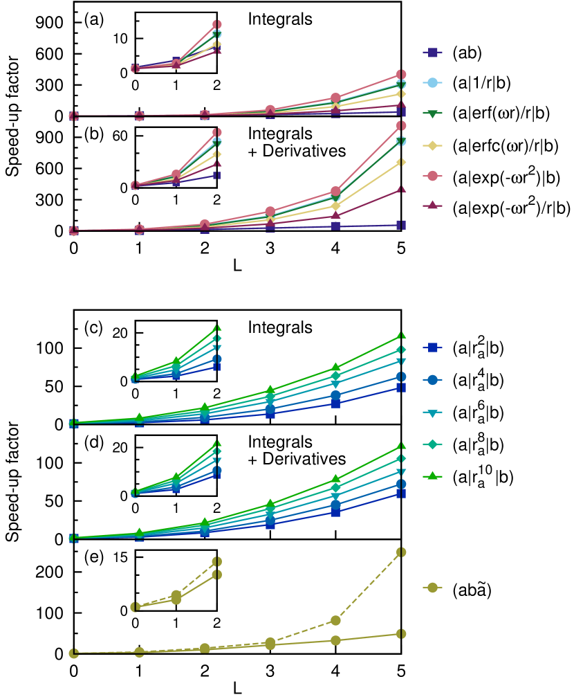
Figure 2: Speed-up for different two-center integrals dependent on the $l$ quantum number at the fixed contraction length $K=7$. The speed-up factor is defined as the ratio OS/SHG. Speed-up for (a,b) integrals $(a|\mathcal{O}|b)$, (c,d) $(a|r_{a}^{2n}|b)$ and (e) $(ab\tilde{a})$. The solid line in (e) is the speed-up for the integrals and the dashed line the speed-up for both, integrals + derivatives.

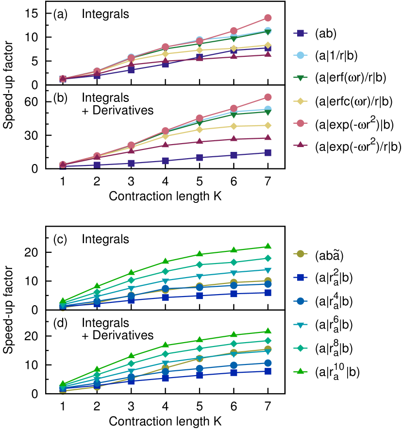
Figure 3: Speed-up for different two-center integrals dependent on the contraction length $K$. The $l$ quantum number is fixed and set to $l=2$. The speed-up factor is defined as the ratio OS/SHG. Speed-up for (a,b) integrals $(a|\mathcal{O}|b)$, (c,d) $(a|r_{a}^{2n}|b)$ and $(ab\tilde{a})$.

Table 3: Speed-up for different two-center integrals. The speed-up is defined as the ratio of the timings OS/SHG. The basis set specifications are given in Table 1.

Integral type	H-DZVP		O-DZVP		O-TZV2PX		Cu-DZVP
	Int.	Int.+Dev.	Int.	Int.+Dev.	Int.	Int.+Dev.	Int.	Int.+Dev.
$(ab)$	$2.4$	$2.4$	$6.2$	$5.5$	$11.4$	$10.3$	$8.9$	$8.3$
$(a|1/r|b)$	$1.8$	$6.2$	$5.9$	$18.4$	$16.8$	$31.6$	$14.6$	$26.0$
$(a|\textnormal{erf}(\omega r)/r|b)$	$1.7$	$6.0$	$5.8$	$18.4$	$16.6$	$31.7$	$14.4$	$26.0$
$(a|\textnormal{erfc}(\omega r)/r|b)$	$1.7$	$5.4$	$5.2$	$16.3$	$14.9$	$29.5$	$12.9$	$24.8$
$(a|\exp(-\omega r^{2})|b)$	$1.8$	$6.7$	$6.4$	$19.7$	$18.0$	$32.5$	$16.0$	$27.4$
$(a|\exp(-\omega r^{2})/r|b)$	$1.6$	$5.0$	$4.4$	$14.1$	$12.3$	$25.4$	$10.8$	$22.0$
$(a|r^{2}_{a}|b)$	$2.6$	$2.7$	$9.7$	$8.8$	$22.9$	$18.6$	$19.7$	$15.8$
$(a|r^{4}_{a}|b)$	$4.0$	$4.0$	$16.0$	$14.0$	$39.4$	$29.3$	$34.7$	$25.2$
$(a|r^{6}_{a}|b)$	$6.6$	$6.3$	$25.3$	$21.6$	$59.5$	$44.3$	$56.1$	$38.9$
$(a|r^{8}_{a}|b)$	$9.1$	$8.1$	$34.7$	$29.6$	$79.3$	$61.4$	$73.4$	$54.6$
$(a|r^{10}_{a}|b)$	$11.8$	$10.5$	$44.7$	$36.7$	$105.2$	$79.9$	$97.5$	$72.2$
$(ab\tilde{a})$	$7.0$	$7.6$	$10.1$	$8.7$	$7.5$	$7.2$	$7.2$	$10.5\par$

Figure 2 displays the performance of the SHG scheme as function of the $l$ quantum number. The speed-up gained by the SHG method is presented for the basis sets TESTBAS_LX for a fixed contraction length. Generally, the ratio of the timings OS/SHG increases with increasing $l$. For the $(a|\mathcal{O}|b)$ integrals, we observe speed-ups between 40 and 400 for $l=5$. For $s$ functions, our method can become up to a factor of two faster. The smallest speed-up is obtained for the overlap integrals since the OS recursion can be spatially separated. The speed-up for the other operators depends on the computational cost for the evaluation of the primitive Gaussian integrals $(0_{a}|\mathcal{O}|0_{b})$. The SHG method outperforms the OS scheme by up to a factor of 1000 ($l=5$) when also the derivatives of $(a|\mathcal{O}|b)$ are computed.

The computational cost for calculating $(a|r_{a}^{2n}|b)$ integrals of $h$ functions is up to two orders of magnitude reduced compared to the OS scheme. The speed-up increases with $n$. The SHG method is beneficial for all $l>0$ and also for $l=0$ when $n\geq 3$. The speed-up factor is generally slightly larger when also the derivatives are required. However, the performance increase is not as pronounced as for the derivatives of $(a|\mathcal{O}|b)$ which is again due to the efficient spatial separation of the OS recurrence.

The performance improvement for $(ab\tilde{a})$ is comparable to the $(a|r_{a}^{2n}|b)$ integrals. For the derivatives of $(ab\tilde{a})$ on the other hand, we get a significantly larger speed-up due to the fact that it increases more than linearly with $l$ and that the OS recurrence has to be performed for larger angular momenta. For instance, the derivatives of the $h$ functions require the recursion up to $l_{a}+l_{\tilde{a}}+1=11$.

Figure 3 shows the performance of the SHG scheme as function of the contraction length $K$. The speed-up increases with $K$ for all integral types. A saturation is observed around $K=6,7$ for $(a|r_{a}^{2n}|b)$ and some of the $(a|\mathcal{O}|b)$ integrals, for example $(a|1/r|b)$. The reason is that the computation of the fundamental integrals $(0_{a}|1/r|0_{b})^{(k)}$ increasingly contributes with $K$ to the total computational cost in the SHG scheme, whereas its relative contribution to the total time is approximately constant in the OS scheme, see Figure S3 (SI). For $K=7$ and $l=2$, the evaluation of $(0_{a}|1/r|0_{b})^{(k)}$ is with 70% the predominant step in the SHG scheme. Since the absolute time for calculating the fundamental integrals is the same in both schemes, the increase in speed-up levels off. The saturation effect is less pronounced, for example, for the overlap $(ab)$ because the evaluation of $(0_{a}0_{b})^{(k)}$ is computationally less expensive than for $(0_{a}|1/r|0_{b})^{(k)}$. Its relative contribution to the total time in the SHG scheme is with 50% significantly smaller, see Figure S3 (d) for $K=7$. However, the saturation for large $K$ is hardly of practical relevance because the contraction lengths of Gaussian basis sets is typically not larger than $K=7$.

The speed-up for separate operations in the integral evaluation can only be assessed for steps such as the contraction, which have an equivalent in the OS scheme. The SHG contraction is increasingly beneficial for large $l$ quantum numbers, large contraction lengths and when also derivatives are computed, see Figure S5 (SI).

Table 3 presents the performance of the SHG method for the MOLOPT basis sets. We find that the SHG scheme is superior to the OS method for all two-center integrals and basis sets. The smallest performance enhancement is obtained for the DZVP basis set of hydrogen, where we get a speed-up by a factor of 1.5-10 because only $s$ and $p$ functions are included in this basis set. A performance improvement of 1-2 orders of magnitude is observed for the basis sets that include also $f$ functions. The largest speed-up is obtained for the $(a|r_{a}^{2n}|b)$ integrals followed by the Coulomb and modified Coulomb integrals. The SHG scheme is even more beneficial, at least for $(a|\mathcal{O}|b)$ integrals, when also the derivatives are computed. For the integrals $(ab)$, $(a|r_{a}^{2n}|b)$ and $(ab\tilde{a})$ on the contrary, the speed-up for both, integrals and derivatives, is instead a bit smaller than for the calculation of the integrals alone. This behavior has to be related to the fact that the MOLOPT basis sets are family basis sets. The OS recursion is carried out for only one set of exponents. Therefore, this part of the calculation is computationally less expensive than for basis sets constituted of several sets of exponents. Furthermore, the OS recursion is computationally less demanding for integrals with local operators, see Section III, and the computational cost for the recursion is in this case only slightly increased when additionally computing the derivatives. In the SHG scheme, the construction of the derivatives from the contracted quantity given in Equation (19) and $\widetilde{Q}^{c/s,c/s}_{l_{a},\mu_{a},l_{b},\mu_{b},j}$ [Equations (45)] and its derivatives [Equations (60)-(62)] is the dominant step for family basis sets. This construction step cannot be supported by memory-optimized library routines and the relative increase in computational cost upon calculating the derivatives is in this particular case larger than for the OS scheme.

For the computation of molecular integrals in quantum chemical simulations, the relation $(a|\mathcal{O}|b)=(-1)^{l_{b}-l_{a}}(b|\mathcal{O}|a)$ can be employed if we have the same set of functions at centers $\mathbf{R}_{a}$ and $\mathbf{R}_{b}$. This relation has not been used for the measurements of the empirical timings, but is in practice useful when the atoms at center $\mathbf{R}_{a}$ and $\mathbf{R}_{b}$ are of the same elemental type.

VI Conclusions

Based on the work of Giese and YorkGiese and York (2008), we used Hobson’s theorem to derive expressions for the SHG integrals $(a|r_{a}^{2n}|b)$ and $(ab\tilde{a})$ and their derivatives. We showed that the SHG overlap $(ab\tilde{a})$ is a sum of $(a|r_{a}^{2n}|b)$ integrals. Additionally, two-center SHG integrals with Coulomb, modified Coulomb and Gaussian operators have been implemented adapting the expressions given in Refs. Ahlrichs, 2006 and Giese and York, 2008.

In the SHG integral scheme, the angular-dependent part is separated from the exponents of the Gaussian primitives. As a consequence, the contraction is only performed for $s$-type auxiliary integrals and their scalar derivatives. The angular-dependent term is obtained by a relatively simple recurrence procedure and can be pre-computed. In contrast to the Cartesian Gaussian-based OS scheme, the derivatives with respect to the spatial directions are computed from lower-order $(l-1)$ terms.

We showed that the SHG integral method is superior to the OS scheme by means of empirical timings. Performance improvements have been observed for all integral types, in particular for higher angular momenta and high contraction lengths. Specifically for the $(a|r_{a}^{2n}|b)$ integrals, the timings ratio OS/SHG grows with increasing $n$. The speed-up is usually even larger for the computation of the Cartesian derivatives. This is especially true for Coulomb-type integrals.

Supplementary Information

Supplementary Material is available for the analytic expressions of $(0_{a}|\mathcal{O}|0_{b})^{(k)}$ employing the standard Coulomb, modified Coulomb and Gaussian-type operators, see Table S1. Further information on integral timings is presented in Figures S1-S5. A detailed description of the MOLOPT basis set is given in Tables S2-S8.

Appendix A Proof of general formula for $\chi_{l,m}(\alpha,\mathbf{r}_{a})r_{a}^{2n}$

In this appendix, we prove that Equation (23) is valid for all $n\in\mathbb{N}$. In the following, the label $tbs$ indicates that the identity of the left-hand side (lhs) and the right-hand side (rhs) of the equation remains to be shown.

Definition 1.

The product of a solid harmonic Gaussian function at center $\mathbf{R}_{a}$ multiplied with the operator $r_{a}^{2n}$ is defined as

$$\chi_{l,m}(\alpha,\mathbf{r}_{a})r_{a}^{2n}:=C_{l,m}(\mathbf{r}_{a})\exp{\left(-\alpha r_{a}^{2}\right)}r_{a}^{2n},$$ (65)

where $C_{l,m}$ is the solid harmonic defined in Equation (2) and $n\in\mathbb{N}$.

Recall that $C_{l,m}(\nabla_{a})$ is the spherical tensor gradient operator (STGO) acting on center $\mathbf{R}_{a}$. In the following we generally drop all ‘passive’ indices, writing e. g. $\textup{I}_{n}$ instead of $\textup{I}_{n}^{l,m,\alpha,\mathbf{r}_{a}}$.

Theorem 1.

Equation (23),

$$\begin{split}\chi_{l,m}(\alpha,\mathbf{r}_{a})r_{a}^{2n}=\frac{C_{l,m}(\nabla_{a})}{(2\alpha)^{l}}\sum_{j=0}^{n}&\binom{n}{j}\frac{(l+j-1)!}{(l-1)!\alpha^{j}}\\ &\times\exp{\left(-\alpha r_{a}^{2}\right)}r_{a}^{2(n-j)}.\end{split}$$ (66)

is valid for all $n\in\mathbb{N}$ .

Proof.

Using Hobson’s theoremHobson (1892) yields

$$\begin{split}C_{l,m}&(\nabla_{a})\exp{\left(-\alpha r_{a}^{2}\right)}r_{a}^{2n}\\ &=(-2)^{l}C_{l,m}(\mathbf{r}_{a})\left(\frac{d}{dr_{a}^{2}}\right)^{l}\left[\exp{\left(-\alpha r_{a}^{2}\right)}r_{a}^{2n}\right].\end{split}$$ (67)

By applying Leibniz’s rule of differentiation we get

$$\begin{split}&\left(\frac{d}{dr_{a}^{2}}\right)^{l}\exp{\left(-\alpha r_{a}^{2}\right)}r_{a}^{2n}\\ &=\sum_{j=0}^{\mathrm{min}(l,n)}\!\binom{l}{j}\!\left[\left(\frac{d}{dr_{a}^{2}}\right)^{l-j}\exp{(-\alpha r_{a}^{2})}\right]\left[\left(\frac{d}{dr_{a}^{2}}\right)^{j}\left(r_{a}^{2}\right)^{n}\right]\\ &=\sum_{j=0}^{\mathrm{min}(l,n)}\binom{l}{j}(-\alpha)^{l-j}\exp{(-\alpha r_{a}^{2})}\frac{n!}{(n-j)!}\left(r_{a}^{2}\right)^{n-j}\\ &=\sum_{j=0}^{\mathrm{min}(l,n)}\binom{n}{j}\frac{l!}{(l-j)!}(-\alpha)^{l-j}\exp{(-\alpha r_{a}^{2})}\left(r_{a}^{2}\right)^{n-j}.\end{split}$$ (68)

Inserting the last line of Equation (68) in Equation (67) and writing out the term for $j=0$ explicitly leads to

$$\begin{split}C_{l,m}&(\nabla_{a})\exp{\left(-\alpha r_{a}^{2}\right)}r_{a}^{2n}\\ ={}&(-2)^{l}(-\alpha)^{l}\exp{(-\alpha r_{a}^{2})}\left(r_{a}^{2}\right)^{n}C_{l,m}(\mathbf{r}_{a})\\ &+(-2)^{l}\sum_{j=1}^{\mathrm{min}(l,n)}\binom{n}{j}\frac{l!}{(l-j)!}(-\alpha)^{l-j}\\ &\quad\times\exp{(-\alpha r_{a}^{2})}\left(r_{a}^{2}\right)^{n-j}C_{l,m}(\mathbf{r}_{a}).\end{split}$$ (69)

Employing Definition 65 and solving for $\chi_{l,m}(\alpha,\mathbf{r}_{a})r_{a}^{2n}$ we obtain

$$\begin{split}\chi_{l,m}&(\alpha,\mathbf{r}_{a})r_{a}^{2n}\\ ={}&\frac{C_{l,m}(\nabla_{a})}{(2\alpha)^{l}}\exp{\left(-\alpha r_{a}^{2}\right)}r_{a}^{2n}-\sum_{j=1}^{\mathrm{min}(l,n)}\binom{n}{j}\frac{l!}{(l-j)!}\\ &\times(-\alpha)^{-j}\exp{(-\alpha r_{a}^{2})}\left(r_{a}^{2}\right)^{n-j}C_{l,m}(\mathbf{r}_{a}).\end{split}$$ (70)

Introducing the notation

$$\textup{I}_{n}:=\chi_{l,m}(\alpha,\mathbf{r}_{a})r_{a}^{2n}$$ (71)

and recalling Definition 65, we obtain a recursion relation:

$$\begin{split}\textup{I}_{n}=&\frac{C_{l,m}(\nabla_{a})}{(2\alpha)^{l}}\exp{\left(-\alpha r_{a}^{2}\right)}r_{a}^{2n}\\ &-\sum_{j=1}^{\mathrm{min}(l,n)}\binom{n}{j}\frac{l!}{(l-j)!}(-\alpha)^{-j}\textup{I}_{n-j}.\end{split}$$ (72)

Furthermore, it is easy to see (applying Hobson’s theorem as done above for general $n$) that

$$\textup{I}_{0}=\frac{C_{l,m}(\nabla_{a})}{(2\alpha)^{l}}\exp{\left(-\alpha r_{a}^{2}\right)}.$$ (73)

From here, the theorem can in principle be obtained by using (72) and (73) recursively. This is made mathematically rigorous by an induction proof in Lemma 2 below. ∎

Let us denote the rhs of (66) by $\textup{II}_{n}$,

$$\textup{II}_{n}:=\frac{C_{l,m}(\nabla_{a})}{(2\alpha)^{l}}\sum_{j=0}^{n}\binom{n}{j}\frac{(l+j-1)!}{(l-1)!\alpha^{j}}\exp{\left(-\alpha r_{a}^{2}\right)}r_{a}^{2(n-j)}.$$ (74)

The following Lemma tells us that the recursive representation (72)-(73) indeed has its closed form given by $\textup{II}_{n}$.

Lemma 2.

For all $n\in\mathbb{N}$ we have

$$\textup{I}_{n}=\textup{II}_{n}.$$ (75)

Proof.

This is proved by mathematical induction.
1. Basis: Recalling (73), it obviously holds $\textup{I}_{0}=\textup{II}_{0}$.
2. Induction Hypothesis: we assume that $\textup{I}_{i}=\textup{II}_{i}$ for all natural numbers $i<n$.
3. Inductive Step: We use the recursion relation (72). Since we sum over $j\geq 1$, we can use the induction hypothesis $\textup{I}_{n-j}=\textup{II}_{n-j}$ to get

$$\begin{split}\textup{I}_{n}={}&\frac{C_{l,m}(\nabla_{a})}{(2\alpha)^{l}}\exp{\left(-\alpha r_{a}^{2}\right)}r_{a}^{2n}\\ &-\sum_{j=1}^{\mathrm{min}(l,n)}\binom{n}{j}\frac{l!}{(l-j)!}(-\alpha)^{-j}\textup{II}_{n-j}.\end{split}$$ (76)

Inserting the definition of $\textup{II}_{n-j}$ (i. e. Equation (74) for $n-j$) this becomes

$$\begin{split}\textup{I}_{n}={}&\frac{C_{l,m}(\nabla_{a})}{(2\alpha)^{l}}\exp{\left(-\alpha r_{a}^{2}\right)}r_{a}^{2n}\\ &-\sum_{j=1}^{\mathrm{min}(l,n)}\binom{n}{j}\frac{l!}{(l-j)!}(-\alpha)^{-j}\frac{C_{l,m}(\nabla_{a})}{(2\alpha)^{l}}\\ &\times\sum_{k=0}^{n-j}\binom{n-j}{k}\frac{(l+k-1)!}{(l-1)!\alpha^{k}}\exp{\left(-\alpha r_{a}^{2}\right)}r_{a}^{2(n-j-k)}.\end{split}$$ (77)

In the following, it is shown that Equation (77) is indeed equal to $\textup{II}_{n}$. All terms of $\textup{I}_{n}$ with $j>0$ in Equation (77) are denoted by

$$\begin{split}\textup{I}_{n}^{\prime}:=&-\sum_{j=1}^{\mathrm{min}(l,n)}\binom{n}{j}\frac{l!}{(l-j)!}(-\alpha)^{-j}\frac{C_{l,m}(\nabla_{a})}{(2\alpha)^{l}}\\ &\times\sum_{k=0}^{n-j}\binom{n-j}{k}\frac{(l+k-1)!}{(l-1)!\alpha^{k}}\exp{\left(-\alpha r_{a}^{2}\right)}r_{a}^{2(n-j-k)}\end{split}$$ (78)

and the contributions with $j>0$ to $\textup{II}_{n}$ in Equation (74) are in the following referred to as

$$\textup{II}_{n}^{\prime}:=\frac{C_{l,m}(\nabla_{a})}{(2\alpha)^{l}}\sum_{j=1}^{n}\binom{n}{j}\frac{(l+j-1)!}{(l-1)!\alpha^{j}}\exp{\left(-\alpha r_{a}^{2}\right)}r_{a}^{2(n-j)}.$$ (79)

To prove that $\textup{I}_{n}=\textup{II}_{n}$, it is sufficient to show that $\textup{I}_{n}^{\prime}=\textup{II}_{n}^{\prime}$. Both sides are reduced to

$$\begin{split}-\sum_{j=1}^{\mathrm{min}(l,n)}&\binom{n}{j}\frac{l!}{(l-j)!}(-\alpha)^{-j}\\ &\times\sum_{k=0}^{n-j}\binom{n-j}{k}\frac{(l+k-1)!}{\alpha^{k}}r_{a}^{2(n-j-k)}\\ \stackrel{{\scriptstyle\mathrm{tbs}}}{{=}}&\sum_{j=1}^{n}\binom{n}{j}\frac{(l+j-1)!}{\alpha^{j}}r_{a}^{2(n-j)}\end{split}$$ (80)

where we denote the lhs by

$$\begin{split}\textup{I}_{n}^{\prime\prime}:={}&-\sum_{j=1}^{\mathrm{min}(l,n)}\binom{n}{j}\frac{l!}{(l-j)!}(-\alpha)^{-j}\\ &\times\sum_{k=0}^{n-j}\binom{n-j}{k}\frac{(l+k-1)!}{\alpha^{k}}r_{a}^{2(n-j-k)}.\end{split}$$ (81)

In order to sort by the exponents of $r_{a}^{2}$ in expression $\textup{I}_{n}^{\prime\prime}$, the Kronecker delta $\delta_{m,j+k}$ is introduced.

$$\begin{split}\textup{I}_{n}^{\prime\prime}={}&\sum_{m=1}^{n}r^{2(n-m)}_{a}\Biggl{(}-\sum_{j=1}^{\mathrm{min}(l,m)}\binom{n}{j}\frac{l!}{(l-j)!}(-\alpha)^{-j}\\[5.0pt] &\times\sum_{k=0}^{n-j}\binom{n-j}{k}\frac{(l+k-1)!}{\alpha^{k}}\delta_{m,j+k}\Biggr{)}.\end{split}$$ (82)

The range of the newly introduced sum is $m=1,...,n$ since for the lower bound of summation we find that $m=j+k\geq 1+0=1$ and for the upper bound $m=j+k\leq j+(n-j)=n$. For the inner sum over indices $j$, it must be considered that $k=m-j$ is negative if $j>m$ while the lower bound of the $k$-sum is in fact $k\geq 0$. Thus, the upper range of the summation of the $j$-sum has to be changed to $\mathrm{min}(l,n,m)$, which is equivalent to $\mathrm{min}(l,m)$ because $m\leq n$. The summation ranges for the innermost sum are not modified since $k=m-j\leq n-j$. In the next step, the $k$-sum is eliminated replacing $k$ by $m-j$,

$$\begin{split}\textup{I}_{n}^{\prime\prime}={}&\sum_{m=1}^{n}\Biggr{(}-\sum_{j=1}^{\mathrm{min}(l,m)}\binom{n}{j}\frac{l!}{(l-j)!}(-\alpha)^{-j}\\[5.0pt] &\times\binom{n-j}{m-j}\frac{(l+m-j-1)!}{\alpha^{m-j}}\Biggr{)}r^{2(n-m)}_{a}.\end{split}$$ (83)

Renaming the summation index on the rhs of Equation (80), we get

$$\textup{II}_{n}^{\prime\prime}:=\sum_{m=1}^{n}\binom{n}{m}\frac{(l+m-1)!}{\alpha^{m}}r^{2(n-m)}_{a}.$$ (84)

We are done if we can show that $\textup{I}_{n}^{\prime\prime}=\textup{II}_{n}^{\prime\prime}$. We do this by comparing summand by summand, i. e. we have to show that for each $m=1,\ldots,n$,

$$\begin{split}-\sum_{j=1}^{\mathrm{min}(l,m)}&\binom{n}{j}\frac{l!}{(l-j)!}(-\alpha)^{-j}\binom{n-j}{m-j}\\ &\times\frac{(l+m-j-1)!}{\alpha^{m-j}}\\ \stackrel{{\scriptstyle\mathrm{tbs}}}{{=}}{}&\binom{n}{m}\frac{(l+m-1)!}{\alpha^{m}}.\end{split}$$ (85)

Expansion of the binomial coefficients and further reduction gives

$$\sum_{j=1}^{\mathrm{min}(l,m)}(-1)^{j+1}\binom{l}{j}\frac{(l+m-j-1)!}{(m-j)!}\stackrel{{\scriptstyle\mathrm{tbs}}}{{=}}\frac{(l+m-1)!}{m!}.$$ (86)

The term on the rhs is in fact the negative of the ‘missing’ summand $j=0$ on the lhs and thus we have

$$\sum_{j=0}^{\mathrm{min}(l,m)}(-1)^{j+1}\binom{l}{j}\frac{(l+m-j-1)!}{(m-j)!}\stackrel{{\scriptstyle\mathrm{tbs}}}{{=}}0.$$ (87)

The lhs is indeed zero, which is easily rationalized by dividing Equation (87) by $(-1)$ and assuming that $\mathrm{min}(l,m)=l$,

$$\sum_{j=0}^{l}(-1)^{j}\binom{l}{j}\frac{(l+m-j-1)!}{(m-j)!}\stackrel{{\scriptstyle\mathrm{tbs}}}{{=}}0,$$ (88)

which is true by Lemma 91. In order to show that the lhs of Equation (87) is also zero for $\mathrm{min}(l,m)=m$, Equation (86) is reformulated

$$\sum_{j=1}^{\mathrm{min}(l,m)}(-1)^{j+1}\binom{m}{j}\frac{(l+m-j-1)!}{(l-j)!}\stackrel{{\scriptstyle\mathrm{tbs}}}{{=}}\frac{(l+m-1)!}{l!}$$ (89)

The term on the rhs is again the ‘missing’ summand for $j=0$ leading to

$$\sum_{j=0}^{m}(-1)^{j}\binom{m}{j}\frac{(l+m-j-1)!}{(l-j)!}\stackrel{{\scriptstyle\mathrm{tbs}}}{{=}}0,$$ (90)

which is again true by Lemma 91 for $m\leq l$. ∎

It remains to prove the following combinatoric identity, which we used in the proof of Lemma 2.

Lemma 3.

For all $l,m\in\mathbb{N}$, $l\leq m$ it holds that

$$0=\sum_{j=0}^{l}(-1)^{j}\binom{l}{j}\frac{(l+m-j-1)!}{(m-j)!}.$$ (91)

Proof.

For all $l\in\mathbb{N}$ and $x\in\mathbb{R}$ we can employ the binomial formula

$$\left(1+\frac{1}{x}\right)^{l}=\sum_{j=0}^{l}\binom{l}{j}\frac{1}{x^{j}}.$$ (92)

Multiplication with $x^{l+m-1}$ on both sides yields

$$x^{l+m-1}\left(1+\frac{1}{x}\right)^{l}=\sum_{j=0}^{l}\binom{l}{j}x^{l+m-j-1}.$$ (93)

The procedure is as follows: we take the $(l-1)$-th derivative with respect to $x$ on both sides and then set $x=-1$. The lhs of Equation (93) is in the following denoted as

$$\textup{III}(x):=x^{l+m-1}\left(1+\frac{1}{x}\right)^{l}$$ (94)

and the rhs is

$$\textup{IV}(x):=\sum_{j=0}^{l}\binom{l}{j}x^{l+m-j-1}.$$ (95)

Applying the Leibniz rule of differentiation to III yields

$$\begin{split}\left(\frac{d}{dx}\right)^{l-1}\textup{III}(x)=\sum_{j=0}^{l-1}\binom{l-1}{j}&\left[\left(\frac{d}{dx}\right)^{l-1-j}x^{l+m-1}\right]\\[1.99997pt] \times&\left[\left(\frac{d}{dx}\right)^{j}\left(1+\frac{1}{x}\right)^{l}\right]\end{split}$$ (96)

Each of the terms in this sum contains a factor $(1+1/x)^{p}$ where $p\geq 1,p\in\mathbb{N}$ since we take no more than $l-1$ derivatives. Setting $x=-1$, the factor $(1+1/x)^{p}$ becomes zero, i.e.

$$\left(\frac{d}{dx}\right)^{l-1}\textup{III}(-1)=0.$$ (97)

Taking the $(l-1)$-th derivative of IV yields

$$\left(\frac{d}{dx}\right)^{l-1}\textup{IV}(x)=\sum_{j=0}^{l}\binom{l}{j}\frac{(l+m-j-1)!}{(m-j)!}x^{m-j}.$$ (98)

Notice that $m-j\geq 0$ since $m\geq l$ and $j\leq l$. By inserting $x=-1$, we get

$$\left(\frac{d}{dx}\right)^{l-1}\textup{IV}(-1)=\sum_{j=0}^{l}\binom{l}{j}\frac{(l+m-j-1)!}{(m-j)!}(-1)^{m-j}.$$ (99)

Putting the lhs, Equation (97), and the rhs, Equation (99), together and dividing both sides by $(-1)^{m}$ yields Equation (91). ∎

Appendix B Proof of general formula for $(0_{a}|r_{a}^{2m}|0_{b})$

In this appendix, we prove that Equation (28) is valid for all $m\in\mathbb{N}$.

Theorem 4.

Equation (28),

$$(0_{a}|r_{a}^{2m}|0_{b})=\frac{\pi^{3/2}\exp(-\rho R_{ab}^{2})}{2^{m}c^{m+3/2}}\sum_{j=0}^{m}I_{j}^{\alpha,\beta,m}(R_{ab}^{2})$$

is valid for all $m\in\mathbb{N}$.

Proof.

The matrix element $(0_{a}|r_{a}^{2m}|0_{b})$ as given in Equation (27) can be rewritten as

$$(0_{a}|r_{a}^{2m}|0_{b})=\exp(-\rho R_{ab}^{2})\int\exp(-cr_{p}^{2})r_{a}^{2m}d\mathbf{r},$$ (100)

where $\rho=\alpha\beta/c$, $c=\alpha+\beta$, $\mathbf{r}_{p}=\mathbf{r}-\mathbf{R}_{p}$ and

$$\mathbf{R}_{p}=\frac{\alpha\mathbf{R}_{a}+\beta\mathbf{R}_{b}}{c}\,.$$ (101)

This is clear by inserting Equation (1) and $Y_{0,0}(\theta,\phi)=\frac{1}{\sqrt{4\pi}}$ into Equation (27) and applying the Gaussian product rule

$$\exp(-\alpha r_{a}^{2})\exp(-\beta r_{b}^{2})=\exp(-\rho R_{ab}^{2})\exp(-cr_{p}^{2}).$$ (102)

Now we define the integral over a primitive $s$ function at center $\mathbf{R}_{p}$ multiplied with the operator $r_{a}^{2m}$ as

$$\textup{V}_{m}:=\int\exp(-cr_{p}^{2})r_{a}^{2m}d\mathbf{r},$$ (103)

where $m\in\mathbb{N}$. Note that we have dropped the indices writing $\textup{V}_{m}$ instead of $\textup{V}_{m}^{\alpha,\beta,\mathbf{r}_{a},\mathbf{r}_{b}}$. In the remainder of this proof, we explicitly calculate this Gaussian integral.

We start by rewriting the operator $r_{a}^{2m}$ in expression $\textup{V}_{m}$ in terms of $\mathbf{R}_{pa}=\mathbf{R}_{p}-\mathbf{R}_{a}$,

$$\textup{V}_{m} =\int\exp(-cr_{p}^{2})\left|\mathbf{r}-\mathbf{R}_{p}+\mathbf{R}_{p}-\mathbf{R}_{a}\right|^{2m}d\mathbf{r}$$ (104)

$$=\int\exp(-cr_{p}^{2})\left[r_{p}^{2}+2\mathbf{r}_{p}\cdot\mathbf{R}_{pa}+R_{pa}^{2}\right]^{m}d\mathbf{r}_{p}.$$ (105)

where $R_{pa}=|\mathbf{R}_{pa}|$. Employing a trinomial expansion yields

$$\begin{split}\textup{V}_{m}=\int&\exp(-cr_{p}^{2})\sum_{\begin{subarray}{c}i+j+k=m\\ i,j,k\in\mathbb{N}\end{subarray}}\binom{m}{i,j,k}r_{p}^{2i}\\ &\times 2^{j}(\mathbf{r}_{p}\cdot\mathbf{R}_{pa})^{j}R_{pa}^{2k}d\mathbf{r}_{p},\end{split}$$ (106)

where the multinomial coefficient is defined as

$$\binom{m}{i,j,k}:=\frac{m!}{i!j!k!}\,.$$ (107)

Introducing the unit vector $\mathbf{\hat{R}}_{pa}$ in direction of $\mathbf{R}_{pa}$ yields

$$\begin{split}\textup{V}_{m}=&\sum_{i+j+k=m}2^{j}\binom{m}{i,j,k}R_{pa}^{2k}|\mathbf{R}_{pa}|^{j}\\ &\times\int\exp(-cr_{p}^{2})r_{p}^{2i}(\mathbf{r}_{p}\cdot\mathbf{\hat{R}}_{pa})^{j}d\mathbf{r}_{p}.\end{split}$$ (108)

Because of rotational symmetry, the integral can not depend on the direction of $\mathbf{R}_{pa}$. So without loss of generality we can take $\mathbf{\hat{R}}_{pa}=\mathbf{e}_{z}$, where $\mathbf{e}_{z}$ is the unit vector in $z$ direction. In order to remove parameter $c$ from the integral, we substitute $\mathbf{r}_{c}:=\sqrt{c}\mathbf{r}_{p}$,

$$\begin{split}\textup{V}_{m}=&\sum_{i+j+k=m}2^{j}\binom{m}{i,j,k}R_{pa}^{2k+j}c^{-\frac{3}{2}-i-\frac{j}{2}}\\ &\quad\times\int\exp(-r_{c}^{2})r_{c}^{2i}(\mathbf{r}_{c}\cdot\mathbf{e}_{z})^{j}d\mathbf{r}_{c}.\end{split}$$ (109)

$\textup{V}_{m}$ is non-zero only for even $j$ (since for odd $j$ the integrand is odd with respect to the reflection of $\mathbf{r}_{c}$ onto $-\mathbf{r}_{c}$) and so we can rewrite Equation (109) as follows,

$$\begin{split}\textup{V}_{m}=&\sum_{i+2j+k=m}2^{2j}\binom{m}{i,2j,k}R_{pa}^{2k+2j}c^{-\frac{3}{2}-i-j}\\ &\quad\times\int\exp(-r_{c}^{2})r_{c}^{2i}(\mathbf{r}_{c}\cdot\mathbf{e}_{z})^{2j}d\mathbf{r}_{c}.\end{split}$$ (110)

We introduce spherical coordinates with $\theta$ being the angle between $\mathbf{r}_{c}$ and the $z$-axis, i.e. $\mathbf{r}_{c}\cdot\mathbf{e}_{z}=r_{c}\cos\theta$,

$$\begin{split}\textup{V}_{m}&=\sum_{i+2j+k=m}2^{2j}\binom{m}{i,2j,k}R_{pa}^{2k+2j}c^{-\frac{3}{2}-i-j}\int_{0}^{2\pi}d\phi\\ &\quad\times\int_{0}^{\pi}{\sin\theta(\cos\theta)^{2j}d\theta}\int_{0}^{\infty}r_{c}^{2}\exp(-r_{c}^{2})r_{c}^{2i}r_{c}^{2j}dr_{c}\,.\end{split}$$ (111)

The integrals over $\theta$, $\phi$ and $r_{c}$ are evaluated explicitly. The integral over $\theta$ is obtained by substitution and the integral over $r_{c}$ is tabulated, for example, in Ref Bronshtein et al., 2015.

$$\begin{split}\textup{V}_{m}=&\sum_{i+2j+k=m}2^{j}\binom{m}{i,2j,k}R_{pa}^{2k+2j}c^{-\frac{3}{2}-i-j}\\ &\times\frac{\pi^{3/2}}{1+2j}\frac{(1+2i+2j)!!}{2^{i}}\,.\end{split}$$ (112)

Employing that $\mathbf{R}_{pa}=\beta(\mathbf{R}_{b}-\mathbf{R}_{a})/c$ yields

$$\begin{split}\textup{V}_{m}=&\sum_{i+2j+k=m}2^{j}\binom{m}{i,2j,k}c^{-\frac{3}{2}-i-3j-2k}\frac{\pi^{3/2}}{1+2j}\\ &\quad\times\frac{(1+2i+2j)!!}{2^{i}}\beta^{2k+2j}R_{ab}^{2k+2j}\,.\end{split}$$ (113)

In order to sort the sum by powers of $R_{ab}^{2}$, we introduce the Kronecker delta,

$$\begin{split}\textup{V}_{m}={}&\sum_{l=0}^{m}\sum_{i+2j+k=m}\delta_{l,k+j}2^{j}\binom{m}{i,2j,k}c^{-\frac{3}{2}-m-l}\\[5.0pt] &\times\frac{\pi^{3/2}}{1+2j}\frac{(1+2i+2j)!!}{2^{i}}\beta^{2l}R_{ab}^{2l}\,,\end{split}$$ (114)

where we have also used that $m=i+2j+k$ and $k=l-j$ to manipulate the exponent of $c$. In the next step, the $k$-sum is eliminated by replacing $k$ by $l-j$

$$\begin{split}\textup{V}_{m}=&{}\sum_{l=0}^{m}\sum_{\begin{subarray}{c}i+j=m-l\\ i,j\geq 0;j\leq l\end{subarray}}2^{j}\binom{m}{i,2j,l-j}c^{-\frac{3}{2}-m-l}\\ &\times\frac{\pi^{3/2}}{1+2j}\frac{(1+2i+2j)!!}{2^{i}}\beta^{2l}R_{ab}^{2l}\,.\end{split}$$ (115)

Then the sum over $i=0,...,m$ is eliminated due to the constraint $i=m-j-l$,

$$\begin{split}\textup{V}_{m}=&{}\sum_{l=0}^{m}\sum_{j\geq 0}^{\mathrm{min}(l,m-l)}2^{j}\binom{m}{m-j-l,2j,l-j}c^{-\frac{3}{2}-m-l}\\[5.0pt] &\times\frac{\pi^{3/2}}{1+2j}\frac{(1+2m-2l)!!}{2^{m-j-l}}\beta^{2l}R_{ab}^{2l}\,.\end{split}$$ (116)

To complete the proof, we have to show that (116) can be simplified as

$$\begin{split}\sum_{l=0}^{m}&\sum_{j\geq 0}^{\mathrm{min}(l,m-l)}2^{j}\binom{m}{m-j-l,2j,l-j}c^{-\frac{3}{2}-m-l}\\ &\qquad\times\frac{\pi^{3/2}}{1+2j}\frac{(1+2m-2l)!!}{2^{m-j-l}}\beta^{2l}R_{ab}^{2l}\\[5.0pt] &\stackrel{{\scriptstyle tbs}}{{=}}\frac{\pi^{3/2}}{2^{m}c^{m+3/2}}\sum_{l=0}^{m}2^{l}\frac{(2m+1)!!}{(2l+1)!!}\binom{m}{l}\frac{\beta^{2l}}{c^{l}}R_{ab}^{2l}.\end{split}$$ (117)

It is sufficient to show that each summand $l$ on the lhs is identical to the summand $l$ on the rhs, i.e. after some reduction of both sides we have

$$\begin{split}&(1+2m-2l)!!\sum_{j=0}^{\text{min}(l,m-l)}2^{2j}\binom{m}{m-j-l,2j,l-j}\frac{1}{1+2j}\\ &\stackrel{{\scriptstyle tbs}}{{=}}\frac{(2m+1)!!}{(2l+1)!!}\binom{m}{l}.\end{split}$$ (118)

This is easily shown employing Lemma 119 and the identity $(2n+1)!!=\frac{(2n+1)!}{2^{n}n!}$. ∎

The following identity was used for the proof of Theorem 4.

Lemma 5.

It holds for all $m,l\in\mathbb{N}$ and $l\leq m$ that

$$\begin{split}&\sum_{j=0}^{\text{min}(l,m-l)}2^{2j}\binom{m}{m-j-l,2j,l-j}\frac{1}{1+2j}\\ &\quad=\frac{(2m+1)!}{(2l+1)!(1+2m-2l)!}.\end{split}$$ (119)

Proof.

The hypergeometric function ${}_{2}F_{1}$ is defined as

$${}_{2}F_{1}(a,b;c;z)=\sum_{j=0}^{\infty}\frac{(a)_{j}(b)_{j}}{(c)_{j}}\frac{z^{j}}{j!}\,,$$ (120)

for $a,b,c,z\in\mathbb{R},|z|<1$. Note that this series is also convergent for $z=1$, if $c>0$ and $c>\mathrm{max}(a,b,(a+b))$. The notation $(q)_{j}$ in Equation (120) is the Pochhammer symbol which is defined for $j\in\mathbb{N}$ as

$$(q)_{j}=\left\{\begin{array}[]{lll}1&&j=0\\[5.0pt] q(q+1)\ldots(q+j-1)&&j\geq 1\end{array}\right.\,.$$ (123)

For negative integers $q=-n,n\in\mathbb{N}$, the Pochhammer symbol simplifies to

$$(-n)_{j}=\left\{\begin{array}[]{lll}1&&j=0\\[5.0pt] (-1)^{j}n!/(n-j)!&&1\leq j\leq n\\[5.0pt] 0&&j\geq n+1\end{array}\right.\,.$$ (127)

For positive real values $x\in\mathbb{R}_{>0}$, the Pochhammer symbol is given by

$$(x)_{j}=\frac{\Gamma(x+j)}{\Gamma(x)}\,,$$ (128)

where the Gamma function for $t\in\mathbb{R}_{>0}$ is defined as

$$\Gamma(t)=\int_{0}^{\infty}x^{t-1}e^{-x}\,dx\,.$$ (129)

For positive integers $n\in\mathbb{N}_{>0}$, the Gamma function evaluates to

$$\Gamma(n)=(n-1)!\,.$$ (130)

Moreover, a duplication identityAbramowitz and Stegun (1972) holds for $t\in\mathbb{R}_{>0}$,

$$\Gamma\left(t+{\tfrac{1}{2}}\right)=\frac{2^{1-2t}\sqrt{\pi}\,\Gamma(2t)}{\Gamma(t)}\,.$$ (131)

We denote the lhs of (119) by $\textup{VI}_{m,l}$,

$$\textup{VI}_{m,l}:=\sum_{j=0}^{\text{min}(l,m-l)}2^{2j}\binom{m}{m-j-l,2j,l-j}\frac{1}{1+2j},$$ (132)

and rewrite Equation (132) recalling $l\leq m$:

$$\textup{VI}_{m,l}=\binom{m}{l}\sum_{j=0}^{\mathrm{min}(l,m-l)}\frac{\frac{l!}{(l-j)!}\frac{(m-l)!}{(m-l-j)!}}{2^{-2j}\frac{(2j+1)!}{j!}}\frac{1}{j!}.$$ (133)

Rewriting Equation (133) yields

$$\textup{VI}_{m,l} \overset{\eqref{eq:pochhammer_neg_int}-\eqref{eq:gamma_dupl}}{=} \binom{m}{l}\sum_{j=0}^{\infty}\frac{(-l)_{j}(-(m-l))_{j}}{\left(\frac{3}{2}\right)_{j}}\frac{1}{j!}$$ (134)

$$\overset{\eqref{eq:def_hypergeo}}{=} \binom{m}{l}\,_{2}F_{1}\left(-l,-(m-l);\tfrac{3}{2};1\right)\,.$$ (135)

Since $(-l)_{j}=0$ for $j>l$ and $(-(m-l))_{j}=0$ for $j>m-l$, see Equation (127), we can replace the upper bound $\mathrm{min}(l,m-l)$ by $\infty$ in Equation (134). We use Gauss’ hypergeometric theoremGasper and Rahman (2004) with $a,b\in\mathbb{R}$, $c>0$ and $c>\mathrm{max}(a,b,(a+b))$,

$${}_{2}F_{1}(a,b;c;1)=\frac{\Gamma(c)\Gamma(c-a-b)}{\Gamma(c-a)\Gamma(c-b)}\,,$$ (136)

to evaluate ${}_{2}F_{1}\left(-l,-(m-l);\frac{3}{2};1\right)$ from Equation (135):

$${}_{2}F_{1} \left(-l,-(m-l);\tfrac{3}{2};1\right)$$

$$\overset{\eqref{eq:Gauss_hypergeometric}}{=}\frac{\Gamma\left(\frac{3}{2}\right)\Gamma\left(\frac{3}{2}+m\right)}{\Gamma\left(\frac{3}{2}+l\right)\Gamma\left(\frac{3}{2}+m-l\right)}$$ (137)

$$\overset{\eqref{eq:gamma_dupl}}{=}\frac{\displaystyle\frac{\Gamma(2)}{\Gamma(1)}\frac{\Gamma(2m+2)}{\Gamma(m+1)}}{\displaystyle\frac{\Gamma(2l+2)}{\Gamma(l+1)}\frac{\Gamma(2m-2l+2)}{\Gamma(m-l+1)}}$$ (138)

$$\overset{\eqref{eq:gamma_integer}}{=}\binom{m}{l}^{-1}\frac{(2m+1)!}{(2l+1)!(2m-2l+1)!}\,.$$ (139)

By inserting Equation (139) into Equation (135), we obtain

$$\textup{VI}_{m,l}=\frac{(2m+1)!}{(2l+1)!(1+2m-2l)!}\,.$$ (140)

∎

See pages 1 of supp_info.pdf See pages 2 of supp_info.pdf See pages 3 of supp_info.pdf See pages 4 of supp_info.pdf See pages 5 of supp_info.pdf See pages 6 of supp_info.pdf See pages 7 of supp_info.pdf See pages 8 of supp_info.pdf See pages 9 of supp_info.pdf

References

• Ahlrichs et al. (1989) R. Ahlrichs, M. Bär, M. Häser, H. Horn,  and C. Kölmel, “Electronic structure calculations on workstation computers: The program system turbomole,” Chem. Phys. Lett. 162, 165–169 (1989).
• Hutter et al. (2014) J. Hutter, M. Iannuzzi, F. Schiffmann,  and J. VandeVondele, “CP2K: Atomistic simulations of condensed matter systems,” WIREs Comput Mol Sci 4, 15–25 (2014).
• (3) “Dalton, a molecular electronic structure program, Release Dalton2016.X (2015), see http://daltonprogram.org,” .
• Werner et al. (2012) H.-J. Werner, P. J. Knowles, G. Knizia, F. R. Manby,  and M. Schütz, “Molpro: a general-purpose quantum chemistry program package,” WIREs Comput Mol Sci 2, 242–253 (2012).
• Schmidt et al. (1993) M. W. Schmidt, K. K. Baldridge, J. A. Boatz, S. T. Elbert, M. S. Gordon, J. H. Jensen, S. Koseki, N. Matsunaga, K. A. Nguyen, S. Su, T. L. Windus, M. Dupuis,  and J. A. Montgomery, “General Atomic and Molecular Electronic Structure System,” J. Comput. Chem. 14, 1347–1363 (1993).
• (6) M. J. Frisch, G. W. Trucks, H. B. Schlegel, G. E. Scuseria, M. A. Robb, J. R. Cheeseman, G. Scalmani, V. Barone, B. Mennucci, G. A. Petersson, H. Nakatsuji, M. Caricato, X. Li, H. P. Hratchian, A. F. Izmaylov, J. Bloino, G. Zheng, J. L. Sonnenberg, M. Hada, M. Ehara, K. Toyota, R. Fukuda, J. Hasegawa, M. Ishida, T. Nakajima, Y. Honda, O. Kitao, H. Nakai, T. Vreven, J. A. Montgomery, Jr., J. E. Peralta, F. Ogliaro, M. Bearpark, J. J. Heyd, E. Brothers, K. N. Kudin, V. N. Staroverov, R. Kobayashi, J. Normand, K. Raghavachari, A. Rendell, J. C. Burant, S. S. Iyengar, J. Tomasi, M. Cossi, N. Rega, J. M. Millam, M. Klene, J. E. Knox, J. B. Cross, V. Bakken, C. Adamo, J. Jaramillo, R. Gomperts, R. E. Stratmann, O. Yazyev, A. J. Austin, R. Cammi, C. Pomelli, J. W. Ochterski, R. L. Martin, K. Morokuma, V. G. Zakrzewski, G. A. Voth, P. Salvador, J. J. Dannenberg, S. Dapprich, A. D. Daniels, Ö. Farkas, J. B. Foresman, J. V. Ortiz, J. Cioslowski,  and D. J. Fox, “Gaussian∼09 Revision X,” Gaussian Inc. Wallingford CT 2009.
• Piquemal et al. (2006) J.-P. Piquemal, G. A. Cisneros, P. Reinhardt, N. Gresh,  and T. A. Darden, “Towards a force field based on density fitting,” J. Chem. Phys. 124, 104101 (2006).
• Cisneros, Piquemal, and Darden (2006) G. A. Cisneros, J.-P. Piquemal,  and T. A. Darden, “Generalization of the Gaussian electrostatic model: Extension to arbitrary angular momentum, distributed multipoles, and speedup with reciprocal space methods,” J. Chem. Phys. 125, 184101 (2006).
• Elking, Darden, and Woods (2007) D. Elking, T. Darden,  and R. J. Woods, “Gaussian Induced Dipole Polarization Model,” J. Comput. Chem. 28, 1261–1274 (2007).
• Gresh et al. (2007) N. Gresh, G. A. Cisneros, T. A. Darden,  and J.-P. Piquemal, “Anisotropic, Polarizable Molecular Mechanics Studies of Inter- and Intramolecular Interactions and Ligand-Macromolecule Complexes. A Bottom-Up Strategy,” J. Chem. Theory Comput. 3, 1960–1986 (2007).
• Elking et al. (2010) D. M. Elking, G. A. Cisneros, J.-P. Piquemal, T. A. Darden,  and L. G. Pedersen, “Gaussian Multipole Model (GMM),” J. Chem. Theory Comput. 6, 190–202 (2010).
• Cisneros (2012) G. A. Cisneros, “Application of Gaussian Electrostatic Model (GEM) Distributed Multipoles in the AMOEBA Force Field,” J. Chem. Theory Comput. 8, 5072–5080 (2012).
• Simmonett et al. (2014) A. C. Simmonett, F. C. Pickard, H. F. Schaefer,  and B. R. Brooks, “An efficient algorithm for multipole energies and derivatives based on spherical harmonics and extensions to particle mesh Ewald,” J. Chem. Phys. 140, 184101 (2014).
• Chaudret et al. (2014) R. Chaudret, N. Gresh, C. Narth, L. Lagardère, T. A. Darden, G. A. Cisneros,  and J.-P. Piquemal, “S/G-1: An ab Initio Force-Field Blending Frozen Hermite Gaussian Densities and Distributed Multipoles. Proof of Concept and First Applications to Metal Cations,” J. Phys. Chem. A 118, 7598–7612 (2014).
• Giese et al. (2015) T. J. Giese, M. T. Panteva, H. Chen,  and D. M. York, “Multipolar Ewald Methods, 1: Theory, Accuracy, and Performance,” J. Chem. Theory Comput. 11, 436–450 (2015).
• Koskinen and Mäkinen (2009) P. Koskinen and V. Mäkinen, “Density-functional tight-binding for beginners,” Comput. Mater. Sci. 47, 237–253 (2009).
• Bernstein, Mehl, and Papaconstantopoulos (2002) N. Bernstein, M. J. Mehl,  and D. A. Papaconstantopoulos, “Nonorthogonal tight-binding model for germanium,” Phys. Rev. B 66, 075212 (2002).
• Giese and York (2005) T. J. Giese and D. M. York, “Improvement of semiempirical response properties with charge-dependent response density,” J. Chem. Phys. 123, 164108 (2005).
• Giese and York (2007) T. J. Giese and D. M. York, “Charge-dependent model for many-body polarization, exchange, and dispersion interactions in hybrid quantum mechanical/molecular mechanical calculations,” J. Chem. Phys. 127, 194101 (2007).
• Golze et al. (2013) D. Golze, M. Iannuzzi, M.-T. Nguyen, D. Passerone,  and J. Hutter, “Simulation of Adsorption Processes at Metallic Interfaces: An Image Charge Augmented QM/MM Approach,” J. Chem. Theory Comput. 9, 5086–5097 (2013).
• Giese and York (2016a) T. J. Giese and D. M. York, “Ambient-Potential Composite Ewald Method for ab Initio Quantum Mechanical/Molecular Mechanical Molecular Dynamics Simulation,” J. Chem. Theory Comput. 12, 2611–2632 (2016a).
• Sodt and Head-Gordon (2008) A. Sodt and M. Head-Gordon, “Hartree-Fock exchange computed using the atomic resolution of the identity approximation,” J. Chem. Phys. 128, 104106 (2008).
• Manzer, Epifanovsky, and Head-Gordon (2015) S. F. Manzer, E. Epifanovsky,  and M. Head-Gordon, “Efficient Implementation of the Pair Atomic Resolution of the Identity Approximation for Exact Exchange for Hybrid and Range-Separated Density Functionals,” J. Chem. Theory Comput. 11, 518–527 (2015).
• Ihrig et al. (2015) A. C. Ihrig, J. Wieferink, I. Y. Zhang, M. Ropo, X. Ren, P. Rinke, M. Scheffler,  and V. Blum, “Accurate localized resolution of identity approach for linear-scaling hybrid density functionals and for many-body perturbation theory,” New J. Phys. 17, 093020 (2015).
• Levchenko et al. (2015) S. V. Levchenko, X. Ren, J. Wieferink, R. Johanni, P. Rinke, V. Blum,  and M. Scheffler, “Hybrid functionals for large periodic systems in an all-electron, numeric atom-centered basis framework,” Comput. Phys. Commun. 192, 60–69 (2015).
• Guidon et al. (2008) M. Guidon, F. Schiffmann, J. Hutter,  and J. VandeVondele, “Ab initio molecular dynamics using hybrid density functionals,” J. Chem. Phys. 128, 214104 (2008).
• Perdew, Burke, and Ernzerhof (1996) J. P. Perdew, K. Burke,  and M. Ernzerhof, “Generalized Gradient Approximation Made Simple,” Phys. Rev. Lett. 77, 3865–3868 (1996).
• Ernzerhof, Perdew, and Burke (1997) M. Ernzerhof, J. P. Perdew,  and K. Burke, “Coupling-Constant Dependence of Atomization Energies,” Int. J. Quantum Chem. 64, 285–295 (1997).
• Ernzerhof and Scuseria (1999) M. Ernzerhof and G. E. Scuseria, “Assessment of the Perdew-Burke-Ernzerhof exchange-correlation functional,” J. Chem. Phys. 110, 5029–5036 (1999).
• Becke (1993) A. D. Becke, “Density-functional thermochemistry. III. The role of exact exchange,” J. Chem. Phys. 98, 5648–5652 (1993).
• Lee, Yang, and Parr (1988) C. Lee, W. Yang,  and R. G. Parr, “Development of the Colle-Salvetti correlation-energy formula into a functional of the electron density,” Phys. Rev. B 37, 785–789 (1988).
• Vosko, Wilk, and Nusair (1980) S. H. Vosko, L. Wilk,  and M. Nusair, “Accurate spin-dependent electron liquid correlation energies for local spin density calculations: a critical analysis,” Can. J. Phys. 58, 1200–1211 (1980).
• Heyd, Scuseria, and Ernzerhof (2003) J. Heyd, G. E. Scuseria,  and M. Ernzerhof, “Hybrid functionals based on a screened Coulomb potential,” J. Chem. Phys. 118, 8207–8215 (2003).
• Heyd, Scuseria, and Ernzerhof (2006) J. Heyd, G. E. Scuseria,  and M. Ernzerhof, “Erratum: “Hybrid functionals based on a screened Coulomb potential” [J. Chem. Phys. 118, 8207 (2003)],” J. Chem. Phys. 124, 219906 (2006).
• Krukau et al. (2006) A. V. Krukau, O. A. Vydrov, A. F. Izmaylov,  and G. E. Scuseria, “Influence of the exchange screening parameter on the performance of screened hybrid functionals,” J. Chem. Phys. 125, 224106 (2006).
• Cohen, Mori-Sánchez, and Yang (2007) A. J. Cohen, P. Mori-Sánchez,  and W. Yang, “Development of exchange-correlation functionals with minimal many-electron self-interaction error,” J. Chem. Phys. 126, 191109 (2007).
• Baerends, Ellis, and Ros (1973) E. J. Baerends, D. E. Ellis,  and P. Ros, “Self-consistent molecular Hartree-Fock-Slater calculations I. The computational procedure,” Chem. Phys. 2, 41–51 (1973).
• Guerra et al. (1998) C. F. Guerra, J. G. Snijders, G. te Velde,  and E. J. Baerends, “Towards an order-N DFT method,” Theor. Chem. Acc. 99, 391–403 (1998).
• te Velde et al. (2001) G. te Velde, F. M. Bickelhaupt, E. J. Baerends, C. F. Guerra, S. J. A. van Gisbergen, J. G. Snijders,  and T. Ziegler, “Chemistry with ADF,” J. Comput. Chem. 22, 931–967 (2001).
• Schütt and VandeVondele (2016) O. Schütt and J. VandeVondele, “Machine Learning Adaptive Basis Sets for efficient large scale DFT simulation,” J. Chem. Theory Comput., submitted  (2016).
• Dupuis, Rys, and King (1976) M. Dupuis, J. Rys,  and H. F. King, “Evaluation of molecular integrals over Gaussian basis functions,” J. Chem. Phys. 65, 111–116 (1976).
• Obara and Saika (1986) S. Obara and A. Saika, “Efficient recursive computation of molecular integrals over Cartesian Gaussian functions,” J. Chem. Phys. 84, 3963–3974 (1986).
• Head-Gordon and Pople (1988) M. Head-Gordon and J. A. Pople, “A method for two-electron Gaussian integral and integral derivative evaluation using recurrence relations,” J. Chem. Phys. 89, 5777–5786 (1988).
• Lindh, Ryu, and Liu (1991) R. Lindh, U. Ryu,  and B. Liu, “The reduced multiplication scheme of the Rys quadrature and new recurrence relations for auxiliary function based two-electron integral evaluation,” J. Chem. Phys. 95, 5889–5897 (1991).
• Bracken and Bartlett (1997) P. Bracken and R. J. Bartlett, “Calculation of Gaussian integrals using symbolic manipulation,” Int. J. Quantum Chem. 62, 557–570 (1997).
• Gill, Gilbert, and Adams (2000) P. M. W. Gill, A. T. B. Gilbert,  and T. R. Adams, “Rapid evaluation of two-center two-electron integrals,” J. Comput. Chem. 21, 1505–1510 (2000).
• Ahlrichs (2006) R. Ahlrichs, “A simple algebraic derivation of the Obara-Saika scheme for general two-electron interaction potentials,” Phys. Chem. Chem. Phys. 8, 3072–3077 (2006).
• McMurchie and Davidson (1978) L. E. McMurchie and E. R. Davidson, “One- and two-electron integrals over cartesian gaussian functions,” J. Comput. Phys. 26, 218–231 (1978).
• Helgaker and Taylor (1992) T. Helgaker and P. R. Taylor, “On the evaluation of derivatives of Gaussian integrals,” Theor. Chim. Acta 83, 177–183 (1992).
• Klopper and Röhse (1992) W. Klopper and R. Röhse, “Computation of some new two-electron Gaussian integrals,” Theor. Chim. Acta 83, 441–453 (1992).
• Reine, Tellgren, and Helgaker (2007) S. Reine, E. Tellgren,  and T. Helgaker, “A unified scheme for the calculation of differentiated and undifferentiated molecular integrals over solid-harmonic Gaussians,” Phys. Chem. Chem. Phys. 9, 4771–4779 (2007).
• Dunlap (1990) B. I. Dunlap, “Three-center Gaussian-type-orbital integral evaluation using solid spherical harmonics,” Phys. Rev. A 42, 1127–1137 (1990).
• Dunlap (2001) B. I. Dunlap, “Direct quantum chemical integral evaluation,” Int. J. Quantum Chem. 81, 373–383 (2001).
• Dunlap (2003) B. I. Dunlap, “Angular momentum in solid-harmonic-Gaussian integral evaluation,” J. Chem. Phys. 118, 1036–1043 (2003).
• Hu and Dunlap. (2013) A. Hu and B. I. Dunlap., “Three-center molecular integrals and derivatives using solid harmonic Gaussian orbital and Kohn-Sham potential basis sets,” Can. J. Chem. 91, 907–915 (2013).
• Giese and York (2008) T. J. Giese and D. M. York, “Contracted auxiliary Gaussian basis integral and derivative evaluation,” J. Chem. Phys. 128, 064104 (2008).
• Kuang and Lin (1997a) J. Kuang and C. D. Lin, “Molecular integrals over spherical Gaussian-type orbitals: I,” J. Phys. B: At. Mol. Opt. Phys. 30, 2529–2548 (1997a).
• Kuang and Lin (1997b) J. Kuang and C. D. Lin, “Molecular integrals over spherical Gaussian-type orbitals: II. Modified with plane-wave phase factors,” J. Phys. B: At. Mol. Opt. Phys. 30, 2549–2567 (1997b).
• Reine, Helgaker, and Lindh (2012) S. Reine, T. Helgaker,  and R. Lindh, “Multi-electron integrals,” WIREs Comput Mol Sci 2, 290–303 (2012).
• Weniger and Steinborn (1985) E. J. Weniger and E. O. Steinborn, “A simple derivation of the addition theorems of the irregular solid harmonics, the Helmholtz harmonics, and the modified Helmholtz harmonics,” J. Math. Phys. 26, 664–670 (1985).
• Weniger (2005) J. Weniger, “The Spherical Tensor Gradient Operator,” arXiv:math-ph/0505018v1  (2005).
• Hobson (1892) E. W. Hobson, “On a Theorem in Differentiation, and its application to Spherical Harmonics,” Proc. London Math. Soc. s1-24, 55–67 (1892).
• Giese and York (2016b) T. J. Giese and D. M. York, “A modified divide-and-conquer linear-scaling quantum force field with multipolar charge densities,” in Many-body effects and electrostatics in biomolecules (Pan Stanford Publishing, Singapore, 2016) pp. 1–32.
• Watson et al. (2004) M. A. Watson, P. Sałek, P. Macak,  and T. Helgaker, “Linear-scaling formation of Kohn-Sham Hamiltonian: Application to the calculation of excitation energies and polarizabilities of large molecular systems,” J. Chem. Phys. 121, 2915–2931 (2004).
• Helgaker, Jørgensen, and Olsen (2012) T. Helgaker, P. Jørgensen,  and J. Olsen, Molecular Electron-Structure Theory (Wiley, 2012) pp. 412–414.
• Schlegel and Frisch (1995) H. B. Schlegel and M. J. Frisch, “Transformation between Cartesian and pure spherical harmonic Gaussians,” Int. J. Quantum Chem. 54, 83–87 (1995).
• Hu et al. (2000) A. Hu, M. Staufer, U. Birkenheuer, V. Igoshine,  and N. Rösch, “Analytical evaluation of pseudopotential matrix elements with Gaussian-type solid harmonics of arbitrary angular momentum,” Int. J. Quantum Chem. 79, 209–221 (2000).
• Gaunt (1929) J. A. Gaunt, “The Triplets of Helium,” Phil. Trans. R. Soc. A A228, 151–196 (1929).
• Xu (1996) Y.-L. Xu, “Fast evaluation of the Gaunt coefficients,” Math. Comp. 65, 1601–1612 (1996).
• Pérez-Jordá and Yang (1996) J. M. Pérez-Jordá and W. Yang, “A concise redefinition of the solid spherical harmonics and its use in fast multipole methods,” J. Chem. Phys. 104, 8003–8006 (1996).
• Homeier and Steinborn (1996) H. H. H. Homeier and E. O. Steinborn, “Some properties of the coupling coefficients of real spherical harmonics and their relation to Gaunt coefficients,” J. Mol. Struct. Theochem 368, 31–37 (1996).
• cp (2) “The CP2K developers group, CP2K is freely available from: http://www.cp2k.org/ (accessed August, 2016),” .
• Note (1) Intel® Xeon® E5-2697v3/DDR 2133.
• VandeVondele and Hutter (2007) J. VandeVondele and J. Hutter, “Gaussian basis sets for accurate calculations on molecular systems in gas and condensed phases,” J. Chem. Phys. 127, 114105 (2007).
• Bronshtein et al. (2015) I. N. Bronshtein, K. A. Semendyayev, G. Musiol,  and H. Mühlig, Handbook of Mathematics (Springer, 6th edition, 2015) p. 1100.
• Abramowitz and Stegun (1972) M. Abramowitz and I. A. Stegun, Handbook of Mathematical Functions with Formulas, Graphs, and Mathematical Tables, 9th ed. (Dover Publications, 1972) p. 256.
• Gasper and Rahman (2004) G. Gasper and M. Rahman, Basic Hypergeometric Series (Encyclopedia of Mathematics and its Applications), 2nd ed., edited by R. S. Doran, P. Flajolet, M. Ismail, T.-Y. Lam,  and E. Lutwak (Cambridge University Press, 2004) p. XIV.