BPS spectra and 3-manifold invariants
Abstract:
We provide a physical definition of new homological invariants of 3-manifolds (possibly, with knots) labeled by abelian flat connections. The physical system in question involves a 6d fivebrane theory on times a 2-disk, , whose Hilbert space of BPS states plays the role of a basic building block in categorification of various partition functions of 3d theory : half-index, superconformal index, and topologically twisted index. The first partition function is labeled by a choice of boundary condition and provides a refinement of Chern-Simons (WRT) invariant. A linear combination of them in the unrefined limit gives the analytically continued WRT invariant of . The last two can be factorized into the product of half-indices. We show how this works explicitly for many examples, including Lens spaces, circle fibrations over Riemann surfaces, and plumbed 3-manifolds.
CALT-TH-2016-039
1 Introduction
Can we hear the shape of a drum? Much like harmonics of a musical instrument, spectra of quantum systems contain wealth of useful information. Of particular interest are supersymmetric or the so-called BPS states which, depending on the problem at hand, can manifest themselves either as minimal surfaces, or solutions to partial differential equations, or other “extremal” objects. Thus, a spectrum of BPS states in Calabi-Yau compactifications can be used to reconstruct the geometry of the Calabi-Yau space itself and, as we explain in this paper, spectra of BPS states play a similar role in low-dimensional topology.
The old approach to constructing numerical invariants of 3- and 4-manifolds, as well as the corresponding homological invariants of 3-manifolds, is based on gauge theory. The famous examples are Donaldson-Witten and Seiberg-Witten (SW) invariants of 4- and 3-manifolds, and corresponding instanton and monopole [1] Floer homologies of 3-manifolds. All of them were extensively studied in mathematical literature and have appropriate rigorous definitions that go back to the previous century. The numerical invariants are realized in terms of counting solutions to certain partial differential equations, while the homological invariants build on the ideas of Andreas Floer [2]. In particular, Seiberg-Witten invariants of 4-manifolds had great success distinguishing some homeomorphic but non-diffeomorphic 4-manifolds. And, in the world of 3-manifolds, the so-called Heegaard Floer homology constructed by Ozsvath and Szabo [3] gives a much simpler and non-gauge theoretic definition of a homological invariant, which is believed to be equivalent to the monopole Floer homology.
A seemingly different class of 3-manifold invariants, the so-called Witten-Reshetikhin-Turaev (WRT) invariants [4, 5], comes from a different type of TQFT, which sometimes is called “of Schwarz type” to distinguish it from the TQFTs “of cohomological type” mentioned in the previous paragraph [6]. At the turn of the century, however, the distinction between the two types started to blur and the ideas of the present paper suggest it may even go away completely in the future. In fact, the first hints for this go back to the early work [7, 8, 9, 10] that relates Seiberg-Witten theory in three dimensions to Chern-Simons theory with super gauge group. The latter provides a much simpler invariant compared to the usual Chern-Simons theory, say, with gauge group, due to cancelations between bosonic and fermionic contributions. Therefore, if one can find a 4d TQFT that categorifies Chern-Simons theory in 3d, similar to how 4d SW theory categorifies 3d SW theory, it would help a great deal with the classification problem of smooth 4-manifolds. The first step in constructing such categorification is, of course, to find a homological invariant of 3-manifolds whose (equivariant) Euler characteristic gives the WRT invariant.
The existence of such 4d TQFT was envisioned by Crane and Frenkel [11] more than 20 years ago, and the first evidence came with the advent of knot homology [12, 13, 14] which categorifies WRT invariants of knots and links (realized by Wilson lines in CS theory) in , also known as the colored Jones polynomial. The physical understanding of a homological approach to HOMFLY polynomials was independently initiated in the physics literature in [15], which later led to the physical interpretation of Khovanov-Rozansky homology as certain BPS Hilbert spaces [16, 17, 18, 19] (see e.g. [20, 21] for an overview and an extensive list of references).
The physical construction suggests that there should be a homological invariant that categorifies (in a certain sense) the WRT invariant of general 3-manifolds with knots inside. Namely, such homological invariant can be understood as the BPS sector of the Hilbert space of the 6d theory (that is a theory describing dynamics of coincident M5-branes in M-theory) on with a certain supersymmetry preserving background along . Equivalently, if one first reduces the 6d theory on , it can be understood as the BPS Hilbert space of the effective 3d theory on . On the other hand, if one first compactifies on , one does not get an ordinary 4d gauge theory on like 4d SW gauge theory111Roughly speaking, the effective 4d theory is an infinite KK-like tower on 4d gauge theories. However one needs to appropriately sum it up. The decategorified counterpart of such summation was studied in [22].:
| (1) |
There is another natural SUSY-preserving background on which one can quantize . Since the IR physics of is governed by a non-trivial 3d SCFT, one can consider its radial quantization and study its Hilbert space on . This should provide us with another non-trivial homological invariant of which should have roughly the same level of complexity as the BPS Hilbert space on which categorifies the WRT invariant, but with several advantages due to the presence of operator-state correspondence and no need to specify a boundary condition at .
The set of boundary conditions that one can put at in the path integral can be understood as follows. Let us represent as an elongated cigar, which asymptoically looks like . After compactification of the stack of fivebranes on we obtain 5d maximally supersymmetric gauge theory. The supersymmetric vacua of such theory on (where is the original time direction) are given by flat connections222The choice of such flat connections should not be confused with the choice of flat connections in CS theory on . As will be explained later in detail they are related by S-transform. on . The number of such supersymetric vacua is the same as the number of boundary conditions (cf. [23, 18, 24, 25, 26]). As we will see later, the subset of such boundary conditions that corresponds to abelian flat connections plays an important role; for convenience, here we summarize various clues that all point to a special role of abelian flat connections:
-
•
charges of BPS states in the target space theory [15];
-
•
relation between homological invariants of different rank [27];
-
•
resurgent analysis of complex Chern-Simons theory [22];
-
•
similar analysis of 3d theories (section 2 below);
-
•
Langlands duality for flat connections on 3-manifolds (section 2.10).
Moreover, in this paper we give many examples of -series invariants for various 3-manifolds which exhibit integrality, and in many cases we also write the corresponding homological invariants. All of these invariants are labeled by (connected components of) abelian flat connections; we do not have any such example associated with a non-abelian flat connection.
In this paper we study the relation between such homological invariants and their decategorified counterparts — superconformal indices. The structure described above, of course, will also manifest itself at the level of partition functions, i.e. indices, once we compactify the time on . For some of the examples in this paper for there are no cancellations among states in computing the refined index. In those cases, the homological invariants are faithfully captured by the refined index computation.
The organization of the paper is as follows. In Section 2 we review some results of [27] and summarize general conjectures about homological invariants of closed 3-manifolds mentioned here and their decategorified versions. In Section 3 we consider various examples for which we explicitly verify these conjectures. In Section 4 we extend it to the case of 3-manifolds with knots. Note, the main part of Section 4 is written in jargonish shorthand, using the concepts and notations introduced earlier. Various details and generalizations of this work can be found in the appendices. Thus, Appendix A explains how the WRT invariants of general negative definite plumbed 3-manifolds can be analytically continued away from roots of unity to produce power series in with integer powers and integer coefficients, required for categorification. In Appendix B, we compare the ordinary Khovanov homology of the -th cabling of the unknot in a 3-sphere to the refined partition function of 3d theory in the presence of line operators, cf. Figure 1. Finally, in Appendix C we explain how categorification of the index of relates to categorification of the Turaev-Viro invariants.
2 Fivebranes on 3-manifolds and categorification of WRT invariant
The goal of this section is to introduce the key players and their interrelation. To keep the discussion simple and concrete, we choose the gauge group to be for most of it, and then in section 2.8 briefly comment how everything can be generalized to higher ranks.
2.1 Preliminaries
Before we present a mathematically-friendly summary of our proposal and the physics behind it, we need to introduce some notations, especially those relevant to abelian flat connections that will be central in our discussion.
Consider a closed and connected 3-manifold , with . In order to present the results in full generality, it will be useful to consider the linking pairing on the torsion part of :
| (2) |
where is a 2-chain such that for an integer . Such and exist because is torsion. As usual, denotes the number of intersection points counted with signs determined by the orientation. Note that the linking form provides an isomorphism between and its Pontryagin dual via the pairing .
The Weyl group acts on the elements via . The set of orbits is the set of connected components of abelian flat connections on (i.e., connections in the image of from the embedding ),333It is in fact that is canonically identified with components of abelian flat connections. However, as the distinction between and its dual is only important in section 2.2, we will use the same set of labels for elements in both groups.
| (3) |
It is also useful to introduce a shorthand notation for the stabilizer subgroup:
| (4) |
2.2 partition function of and WRT invariant
Now we are ready to present a slightly generalized and improved version of the results from [27, sec. 6].
Categorification of WRT invaraiant
Let be the partition function of Chern-Simons theory with “bare” level on , also known as the WRT invariant. We use the standard “physics” normalization where
| (5) |
and
| (6) |
The following conjecture was proposed in [27].444A related conjecture was made in [28]. However it did not include the -transform, which is crucial for restoring integrality and categorification.
Conjecture 2.1
The WRT invariant can be decomposed into the following form:
| (7) |
with555The constant positive integer depends only on and in a certain sense measures its “complexity”. In many simple examples , and the reader is welcome to ignore factor which arises from some technical subtleties. Its physical origin will be explained later in the paper.666Later in the text we will sometimes use slightly redefined quantities, , where is a common, independent rational number.
| (8) |
convergent in and
| (9) |
In other words, we claim the existence of new 3-manifold invariants , which admit -series expansion with integer powers and integer coefficients (hence, more suitable for categorification) and from which the WRT invariant can be reconstructed via (7). While the formal mathematical definition of the invariants is waiting to be discovered, they admit a physics definition that will be reviewed below and can be independently computed via techniques of resurgent analysis. In particular, each term
| (10) |
in the sum (7) is a certain resummation of the perturbative (in or, equivalently, in ) expansions of the WRT invariant around the corresponding abelian flat connection [22].
In order to avoid unnecessary technical complications, in the rest of this paper we assume that has no factors.777Recall that , as a finitely generated abelian group, can be decomposed into . We ask for a fairly weak condition that doesn’t appear in this decomposition. In other words, is a -homology sphere. Equivalently, there is a unique Spin structure on , so that there is no ambiguity in specifying Nahm-pole boundary condition for SYM on [18]. The general case, in principle, could also be worked out. We leave it as an exercise to an interested reader. Under this assumption, the -matrix satisfies
| (11) |
Moreover, as will be discussed in detail below, physics predicts the existence of a graded homological invariant of :
| (12) |
which categorifies the -series . Namely888 The presence of factors that produce overall factor in (8) can be interpreted as presence of factors with in . The -graded Euler charecteristic of is naively divergent: , but its zeta-regularization gives . ,
| (13) |
Because of their close relation to homological invariants, we usually refer to as homological blocks. The vector space can be interpreted as the closed 3-manifold analog of Khovanov-Rozansky knot homology. From this point of view, can be understood as the variable associated with grading and enters into the decomposition (7) much like , the variable for one of the -gradings (the “-grading”). Note that the label in is reminiscent of the Spinc structure in Heegaard/monopole Floer homologies of 3-manifolds. This fact, of course, is not an accident and plays an important role in the relation between Heegaard/monopole Floer homologies of 3-manifolds and the categorification of WRT invariants [27].
Next, we describe the physics behind the Conjecture 9. (A mathematically inclined reader may skip directly to Conjecture 20.)
Physics behind the proposal
From physics point of view, the homological invariants can be realized by the following M-theory geometry,
| (14) |
or, equivalently, any of its dual descriptions (some of which will be discussed below). Here, the first two lines summarize the geometry of the fivebranes and their ambient space, whereas the last line describes their symmetries. The reason “” appears in quotes is that it is a symmetry of our physical system only when is a Seifert 3-manifold, unlike the “universal” symmetry group .
In order to preserve supersymmetry for a general metric on , it has to be embedded in the geometry of ambient space-time as a supersymmetric (special Lagrangian) cycle which, according to McLean’s theorem, always looks like near the zero section. Equivalently, the geometry represents a partial topological twist on the fivebrane world-volume, upon which three of the scalar fields on the world-volume become sections of the cotangent bundle of . As a result, one can first reduce the 6d theory — the world-volume theory of M5-branes — on to obtain a 3d SCFT usually denoted as , where or , being the number of M5-branes. All SUSY-protected objects like partition functions, index and BPS spectra of the resulting theory do not depend999A “folk theorem” states that any continuous deformation of the metric on results in a -exact term of the supergravity background. However, there may be dependence on discrete data such as the Atiyah 2-framing [29]. on the metric of , and give rise to numerical as well as homological invariants of .
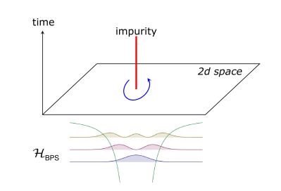
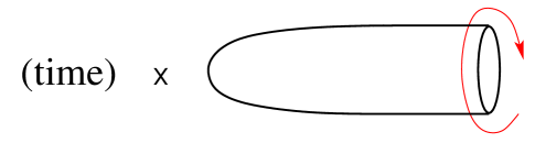
Similarly, in order to preserve supersymmetry of the brane system (14) along the other world-volume directions of the fivebranes, one needs to introduce a SUSY-preserving background along . Moreover, it needs to be done in a way that preserves the rotation symmetry and allows to keep track of the corresponding quantum numbers (spins) of BPS states, as required for categorification. The suitable background can be described in a number of equivalent ways: as the Omega-background along in which is embedded as a linear subspace, or as a invariant Lagrangian submanifold (the “cigar”) in the Taub-NUT space where one keeps track of the spin with respect to the rotation symmetry, cf. Figure 2. To emphasize that one keeps track of both spins under symmetry, the adjective refined is often added to the invariant, BPS state, or other object under consideration.
When is a Seifert manifold, the brane system (14) enjoys an extra symmetry that appears in a degeneration limit of the metric on and can be used to redefine the R-symmetry of the SCFT . When is , the symmetry is further enhanced to the R-symmetry of the 3d theory ; when is a generic Seifert manifold, one combination gives the R-symmetry of the 3d theory which we denote as , while another is a flavor symmetry , see [27, sec. 3.4] for details.
After reduction on , the system (14) gives a theory in space-time , illustrated in Figure 1, and we can consider its Hilbert space with a certain boundary condition at . For and — the case that we will be mostly considering in this paper — these boundary conditions turn out to be labeled by . Then, we arrive at a set of doubly-graded homological invariants of labeled by ,
| (15) |
given by the BPS sector of the Hilbert space of . This is the subspace annihilated by two of the four supercharges of the 3d supersymmetry (different choices are related by automorphisms of the superconformal algebra, resulting in isomorphic BPS spaces). The grading counts the charge under the rotation of and the “homological” grading corresponds to R-charge of the R-symmetry. When is Seifert, the symmetry will give rise to the third grading101010Not to be confused with the extra “HOMFLY grading” e.g. on the right-hand side of (69). on .
One can understand as the massless multi-particle BPS spectrum of with a label being a discrete charge. From M-theory point of view, the BPS particles of arise from M2-branes ending on the pair of M5-branes that realize the 6d theory. The boundaries of M2-branes wrap 1-cycles so that . This is similar to the counting of BPS states in [15]. Note, however, that BPS particles that arise from M2-branes ending on a non-torsion 1-cycles of have mass and do not enter into the IR BPS spectrum. Therefore, it is elements in that give rise to physical boundary conditions which specifies a superselection sector labeled by this brane charge, resulting in a physical BPS Hilbert space with integrality property. In contrast, a flat connection, given by an element of doesn’t correspond to any physical boundary conditions. Instead, it is a linear combination of physical boundary conditions leading to a mixture of different charge sectors.
From this point of view, the S-transform in Conjecture 9 carries out the change of basis between charges (valued in ) and holonomies (valued in ) using the natural pairing between them via the “Aharonov-Bohm phase.” More precisely, the M2-branes ending on M5-branes produce particles in the effective 3d theory carrying electric-magnetic charge .111111Note that in the case of M5-branes wrapping , the M2-branes produce states charged under the magnetic (not necessarily ) symmetry, as explained in [15]. On the other hand, specified the holomony, and, by viewing as the group of characters of , we have
| (16) |
Geometrically, is the trace of the holonomy of the flat connection labeled by along the 1-cycle representing homology class .
Alternatively, one can understand the boundary conditions in the type IIB duality frame of the brane system (14), where S-transform can be interpreted as the S-duality of type IIB string theory. Indeed, a quotient of the eleven-dimensional space-time by a circle action lands us in type IIA string theory, which can be further T-dualized along the “time” circle . (Equivalently, these two dualities can be combined into one step, which is the standard M-theory / type IIB duality.) The resulting system involves D3-branes ending on a D5-brane, and S-duality of type IIB string theory maps it into a stack of D3-branes ending on an NS5-brane [18]. Note, that the natural choice of boundary conditions at infinity for a system of D3-branes ending on an NS5-brane is an arbitrary (not necessarily abelian) flat connection on . Such choice of a flat connection corresponds to considering analytically continued Chern-Simons theory on the Lefschetz thimble associated to that flat connection. However, in general, the corresponding partition function is not continuous in a disk due to Stokes phenomena. Instead, in (10) we consider quantities which are labeled by abelian flat connections only, and analytic inside . As explained in [22], for a given value of one can express as a linear combination of the Feynman path integral on Lefschetz thimbles. If one were to write the S-transform in the basis corresponding to Lefschetz thimbles, instead of , the S-matrix would be -dependent.
By definition, each homological block is the graded Euler characteristics (36) of that can be computed as an supersymmetric partition function of on with an supersymmetric boundary condition and metric corresponding to rotation of the disk by when we go around the ,
| (17) |
If one knows the Lagrangian description of , this partition function can be computed using localization, see e.g. [30].
Note, if the Lagrangian description of contains chiral multiplets charged under the gauge symmetry, carrying zero R-charge (at the unitarity bound) and with Neumann boundary conditions, then the integral computing the partition function (i.e. the half-index) will be singular in general. For example, for adjoint chiral multiplets the partition function has the following form:
| (18) |
A natural way to regularize it is to take the principle value prescription:
| (19) |
As we will see in many examples, this regularization prescription is in agreement with the relation between and the WRT invariant. This is also the source of the factor in (8).121212Such factor can appear even without singularity, when there is only adjoint chiral with R-charge 0. It cancels the contribution of the vector multiplet, leaving (20) where one can take , as an example.
Resurgence in 3d theories
The phenomenon of non-abelian contributions being distributed among the abelian ones can be translated entirely into the language of 3d field theories. In fact, this phenomenon is not limited to theories associated with 3-manifolds and should be regarded more broadly, as a decomposition of BPS quantities in gapless (conformal) theories into BPS spectra of its massive deformations.
Thanks to supersymmetric localization, partition functions of 3d theories on can be reduced to finite-dimensional integrals, which in the limit have the form
| (21) |
The multi-variable typically comes from gauge factors, and can be interpreted as a twisted superpotential of the 3d theory on a circle. Its critical points are the vacua of the 2d effective field theory, which for a finite-size circle come in infinite towers. Indeed, when the 3d theory is compactified on a circle of finite radius, the variables are -valued and the equations for vacua also have the exponentiated form:
| (22) |
For this reason, each vacuum comes in an infinite family, much like saddle points of Chern-Simons functional. Also, as in Chern-Simons theory, the critical points of have the leading order behavior
| (23) |
where the critical exponent is the degree of degeneracy of the critical point ; the larger the value of the more singular the critical point is (see [31] for a careful treatment of such factors).
Therefore, in the context of completely general 3d theories we find two key elements of the resurgent analysis [22]: the critical points come in infinite -towers and they may have different degree of degeneracy signalled by powers of . Hence, applying the resurgent analysis of [22] to the integral (21), we conclude that contributions of critical points with smaller values of the exponent will be “distributed” among critical points with larger values of .
In order to see this phenomenon in physically-motivated 3d theories, such as 3d SQED or SQCD, we simply need to look at examples with non-trivial range of values of .
2.3 Realization in terms of counting solutions of differential equations
In the previous section we defined homological invariants of 3-manifolds as Hilbert spaces of 6d (2,0) theory on where is the time direction. It is possible to give another definition that, in a sense, is closer to the definition of instanton [2] or monopole (Seiberg-Witten) Floer homology of 3-manifolds [1] familiar to many topologists. We will mostly follow [18], where the detailed discussion can be found.
Let us represent as a cigar fibered over with fibers being the orbits of the action rotating the disc (see Figure 2).131313Exchanging the circle fiber of with in (17) has the effect of replacing the group with its GNO/Langlands dual . The tip of the cigar is a degenerate fiber projected to the origin of . The 6d (2,0) theory corresponding to the Lie algebra on then can be effectively described as 5d maximally supersymmetric Yang-Mills theory with gauge group on , topologically twisted along . One can further reduce it to the 2d LG theory on with the target space being the space of flat connections modulo gauge transformations and the superpotential being the holomorphic Chern-Simons functional where is the connection 1-form [32]. The imaginary part originates from three (out of five) adjoint scalar fields in 5d theory that transform as a vector under R-symmetry group and become a one-form on after topological twisting [33, 34]. The boundary condition at the origin of (the image of the cigar under projection) is a Nahm-pole type boundary condition that requires a certain singular behavior of , which in local coordinates takes the following form:
| (24) |
where is the vierbein for some choice of metric on , are the images of the standard generators of under a principal embedding ,141414For (or ) the principal embedding is such that fundamental representation of restricts to an irreducible -dimensional representation of . and is the coordinate along . The real part of the connection obeys the Dirichlet boundary condition that fixes it at to be equal to the spin-connection on via the principal embedding .
There is also a choice of boundary condition at the infinite end of that corresponds to the choice of the boundary condition at the boundary of the disk. As in any 2d Landau-Ginzburg model, there is a natural family of boundary conditions labeled by connected components of the critical points of the superpotential [35]. They are given by Lagrangian branes supported on Lefschetz thimbles associated to those connected components.
The BPS Hilbert space labeled by the connected component
| (25) |
then can be constructed as a Floer homology as follows. As usual, classically the BPS states of the 2d Landau-Ginzburg model on , where is the time direction, are given by solutions of time-independent BPS equations, that is gradient flows with respect to CS functional on with specified boundary conditions. On the quantum level the BPS Hilbert space is given by the cohomology of Morse-Witten complex of such classical BPS states graded by the Morse index. The differential is given in terms of counting solutions of BPS equations interpolating between two time-independent solutions at in the time direction. Such differential equations, when written in terms of 5d theory on are often referred as Haydys-Witten equations[36, 18]. The Hilbert space has two gradings. One is the usual Morse-index/R-charge/homological grading. The other grading, corresponding to the generating variable in the index , is given by the instanton number
| (26) |
Here is the action of the gravitational CS on , which, taking into the account the boundary condition at the origin of , makes the instanton number well defined. Note that this, at least naively, defines for connected components of all flat connections.151515On a closer look, though, there is a significant difference between solutions with abelian and non-abelian flat connections at . When the flat connection is irreducible, the -component of the adjoint-valued Higgs field vanishes and remains zero for all values of , while it is not the case when the flat connection at is reducible. However, in the previous sections, when discussing categorification of WRT invariant, we used only a subset of spaces labeled by connected components of abelian flat connections. The deep reasoning for this phenomenon is yet to be understood, but resurgence theory provides some explanation on the decategorified level at least for some class of 3-manifolds [22].
The definition of given in this section, although quite explicit, is still on the physical level of rigor, and in order to make it mathematically accurate one still has to overcome various problems, such as singularities and compactness of the corresponding moduli spaces. When moduli spaces are not compact, one needs either to find a suitable compactification (which, in the present context, does not spoil topological invariance) or supplement the standard Morse-Floer theory with more powerful tools. Indeed, even at the decategorified level, the “counting” of solutions requires integration over moduli spaces and, even if all problems are solved, may not produce integers. A familiar example is the calculation of Gromov-Witten invariants via integration over the moduli spaces of stable maps, where maps with non-trivial stabilizers lead to rational rather than integer invariants.
The present problem, however, is much more challenging than compactness issues that one encounters in Gromov-Witten or Donaldson-Witten theory. One standard tool that replaces Morse theory in the non-compact setting is the Conley index. While its application to the current problem will be discussed elsewhere, here we can make a few brief comments that resonate with the rest of the present paper. The moduli spaces in question, , depend on the choice of a 3-manifold and the boundary condition at . A generic choice of the boundary condition, of course, will not result in integer invariants (even at the decategorified level) and only particular choices of boundary conditions will lead to moduli spaces where one might hope to address compactness issue without destroying integrality and topological invariance. Our present study suggests that boundary conditions labeled by abelian flat connections are precisely the ones which have this property.
Another issue is that counting the number of solutions of such differential equations, even if properly defined, is computationally very hard. Therefore one should explore other possibilities to mathematically define .
2.4 Surgeries, triangulations, and Atiyah-Floer
In order to give a mathematical formulation of the homological invariants that can be useful for practical calculations on an arbitrary 3-manifold, the starting point must be a construction of the 3-manifold itself. Then, different ways to present the same 3-manifold may lead to different but equivalent definitions of which, in physics, correspond to different ways of looking at the fivebrane system (14).
For example, in addition to its original combinatorial definition [12], the Khovanov homology of knots by now has definitions based on matrix factorizations [13], algebraic geometry [37], symplectic geometry [38, 39, 40], etc. As expected, they are all equivalent [41, 42] and offer different useful perspectives. Similarly, we expect that our homological invariants of 3-manifolds admit several mathematical definitions, thus providing new opportunities and bridges among different areas of mathematics.
A standard way to produce a symplectic definition is based on the Atiyah-Floer conjectures, which relate gauge theory version of Floer homology and its symplectic version (see e.g. [17] for a review and an application in a closely related context). The idea is to represent a 3-manifold as a Heegaard decomposition
| (27) |
of two handlebodies joined by a long “neck” . Then, topological reduction on gives a 2d sigma-model with target space and space-time (“world-sheet”) , with the boundary conditions at the end-points of the interval determined by . Then, the Floer homology of the higher-dimensional theory can be equivalently formulated as a symplectic Floer homology in the topological A-model with target space and two Lagrangian submanifolds and :
| (28) |
As with other candidates for the mathematical definition of , the main challenge is to describe precisely the moduli spaces and . For example, to obtain it is convenient to first reduce 6d theory on times the circle fiber of to obtain a sigma-model with target space , the Hitchin moduli space (in which and cut out holomorphic Lagrangian submanifolds).
Another way to build 3-manifolds is to start with a simpler 3-manifold, say 3-sphere, remove a tubular neighborhood of some knot (or link) and then glue it back in a different way. This operation is called surgery and, in fact, every 3-manifold can be realized as a sequence of surgery operations on a 3-sphere . In view of this, it is natural to ask if 3-manifold homology of the resulting manifold is related to homology of knots and links.
As is well known in the theory of quantum group invariants, at the decategorified level the answer is “yes” and here we argue that this is also true at the homological level. Indeed, a quantum group invariant (WRT invariant) of a 3-manifold obtained by surgery on is completely determined by polynomial invariants of , with a proviso that one needs to know all colored invariants of . In the case of these are colored Jones polynomials and to obtain the WRT invariant of one basically need to sum over color (which is typical for any state sum type models).
Since at present all colored polynomial invariants of have rigorous mathematical definition one could try to write a surgery formula where colored Jones polynomials of are replaced by the corresponding homologies (or their Poincaré polynomials). Surprisingly, in a few examples that we checked this indeed gives the 3-manifold homology , and it is natural to conjecture that this is true in general. If so, one extremely concrete, mathematically well-defined and computable definition of could be via surgery formula and sum over colored knot (link) homologies.
As a concrete example, consider a Lens space constructed as a surgery on the unknot. In fact, this also gives an example of genus- Heegaard splitting since the unknot complement is a solid torus. Let be the Poincaré polynomial of -colored homology categorifying the -colored Jones polynomial . As usual, it is convenient to package all in a single function such that
| (29) |
Put differently, if is the operator that generates recursion relation among , such that and , then [43, 44]:
| (30) |
In terms of the function that packages Poincaré polynomials of colored unknot homology, the Poincaré polynomial of , where , is given by the “Laplace transform” [22, 45, 46] of ,
| (31) |
i.e. by a convolution with the theta-function . Note, all the information about homological grading (that is, -dependence) comes entirely from , i.e. from the colored unknot homology, and not from the Laplace transform that produces 3-manifold invariant out of the knot invariant. In other words, categorification of the surgery formula affects only the Jones polynomial part (by replacing it with the Poincaré polynomial).
Another way to build 3-manifolds and, therefore, another candidate for constructing is based on triangulations. This approach is especially attractive due to its combinatorial nature and has been extensively used as a platform for mathematical definitions of various supersymmetric partition functions of 3d theory , see e.g. [47, 48, 49, 50, 51, 52, 53]. Reducible flat connections, again, are special, for the same reason as before. However, in partition functions, the non-trivial stabilizer of reducible flat connections works against them and formally makes their contribution vanish in a Chern-Simons theory with non-compact gauge group. This has to be contrasted with homological invariants, where redicible solutions produce infinite contributions (e.g. in Heegaard Floer homology) compared to finite contributions of irreducible solutions. This suggests that in partition functions too, both reducible and irreducible contributions can be seen together if we consider framed gauge transformations161616A framed gauged transformation acts trivially at a chosen point on . and then instead of further dividing by work equivariantly. To the best of our knowledge, this has not been done and presents a nice and tractable problem for future work.171717A closely related -equivariant rather than -equivariant regularization of complex Chern-Simons partition function was used [54] for 3-manifolds of the form . As expected, this equivariant localization does help to see contributions of both abelian and non-abelian flat connections in the same partition function.
2.5 Superconformal index of and its factorization
Although the new invariants and their categorification have a direct connection to the WRT invariant via (7), from the viewpoint of 3d theory , it is not the most natural or simplest object to consider. The main reason is that, in principle, there are infinitely many possible boundary conditions that could be considered.181818If we understand the boundary condition as a coupling of the 3d theory to a 2d theory living on the boundary, then the infinite number of possibilities can be seen, for example, from the fact that we can always introduce a 2d theory decoupled from the bulk. Identifying the correct subset that appears in (17) may be subtle, yet possible, as we shall see in concrete examples.
The more natural object is the superconformal index of or, equivalently, the partition function on with a certain supersymmetry preserving background:
| (32) |
where is the space of BPS states of 3d SCFT or, equivalently, -cohomology of all physical local operators, is the fermion number, is the generator of the R-symmetry and is the Cartan generator of the isometry of . By construction, this index has the desired integrality property191919For reasons similar to the ones described at the end of the previous section, in general a negative power of 2 can appear as an overall factor. We omit it in some generic formulas to avoid clutter and instead focus attention on the conceptual structure. As mentioned earlier and as we shall see in examples, the effect of such fractions on categorification can typically be traced to the existence of bosonic modes with zero -grading. and can be categorified,
| (33) |
Another advantage of compared to is that it has a natural ring structure which is given by multiplication of BPS operators. One of the statements of 3d/3d correspondence is that the partition function computes the partition function of complex Chern-Simons on with real part of the “level” being and analytically continued imaginary part . Motivated by the topological/anti-topological fusion [23] and its recent 3d incarnation [24, 25, 26, 55], we would like to make the following conjecture:
Conjecture 2.2
For as in Conjecture 9, the following holds
| (34) |
where is an apropriate extension202020For a generic 3-manifold , the analytic continuation of the series convergent in may not exist outside , at least in the standard way. However, one possible way to define it for general is (35) where denotes with the reversed orientation. Note that therefore , unlike , is insensetive to the orientation. of to the region .
2.6 Further refinement
As we discussed above, for Seifert 3-manifolds the theory has an extra flavor symmetry. In particular, this is the case for , which will serve as an important example to us later. This flavor symmetry in results in the presence of an extra -grading in homological invariants and considered in the previous sections and a possibility to consider the corresponding refined indices (equivariant Euler characteristics):
| (36) |
and
| (37) |
where, from the physics point of view, is the charge. The refined indices obviously provide more information about the underlying vector spaces and, as we will see in examples, can be used sometimes to compute (conjecturally) the full homological invariants via the “homological-flavor locking” phenomenon that we will explain later.
The refined version of the factorization formula (34) reads
| (38) |
2.7 Topologically twisted index of
Another interesting invariant of which can be realized as an observable of and has a categorification by construction is the topologically twisted index on [56]. Namely, one can consider the 3d theory with a background value of the -symmetry connection equal to the spin connection on . In terms of the effective 2d theory obtained by compactifying on , this is the familiar A-twist along the .
The topologically twisted index and the underlying homological invariant of have the same fugacities/gradings as the superconformal index:
| (39) |
As in the superconformal index , here the parameter plays the role of the Omega-background parameter corresponding to rotating along one of the axes. However, in general the topologically twisted index has a much simpler structure (as will be explained later) compared to the superconformal index . Namely, is a rational function of (i.e. it has a form of the index of quantum mechanics with two supercharges), whereas can be as transcendental as, say, a quantum dilogarithm or (Jacobi) mock modular form. Nevertheless, the topologically twisted index is expected to have a similar factorization into homological blocks:
| (40) |
The difference from (38) is due to the fact that the supersymmetric backround chosen for superconformal index can be interpreted as doing topological A-twist along one of the halves and anti-A-twist along the other half,
| (41) |
whereas the background for the topologically twisted index is such that the same A-twist is performed along both halves:
| (42) |
2.8 Generalization to
For simplicity, in this paper we mostly consider Chern-Simons theory on with gauge group being and the 3d/3d dual theory . However, in principle, everything we say above and below for can be easily generalized to the or case; there are no obstructions for that. In particular, the formulae appearing in Conjecture 9 generalize as follows for :
| (43) |
| (44) |
| (45) |
| (46) |
As before, using the linking pairing one can identify with the set of connected components of abelian flat connections:
| (47) |
where is the permutation group of a set with elements. The factorization formulae (38) and (40) generalize as follows
| (48) |
| (49) |
with
| (50) |
Physically, there are several ways to understand the special role of abelian flat connections or, more generally, reducible flat connections for of higher rank. As we already mentioned in section 2.2, from the viewpoint of quantum field theory (on fivebrane world-volume or its various reductions and limits) this follows directly from the resurgent analysis. On the other hand, by looking at the same system (14) from the vantage point of the Calabi-Yau 3-fold, the set (47) which labels the new invariants and their categorification can be understood as charges of the BPS states or enumerative invariants of the Calabi-Yau 3-fold. We elaborate on this perspective in the following two subsections, expanding the web of dualities and interpretations.
2.9 Relation to open GW invariants on
Consider level- Chern-Simon theory on a rational homology sphere ,
| (51) |
i.e. is a finite abelian group. (What follows can be considered as a generalization from the case considered in [57]).
Similar to the case, is the Chern-Simons invariant of the abelian flat connection , and is a Borel resummation [22] of the asymptotic expansion around . Correspondingly, is a Borel resummation of the series of the following type:
| (52) |
Consider
| (53) |
as a formal variable in a generating series. Then , for each , up to a factor, can be viewed as a basis element of the symmetric part of the group ring212121For example, when and we have: (54) and (55) where . of :
| (56) |
if we identify
| (57) |
in the group ring of .
Then
| (58) |
while
| (59) |
On the other hand, one can consider open topological strings (A-model) on with a Lagrangian brane along equipped with a rank- bundle and an abelian flat connection (local system) . The free energy is given by
| (60) |
where the open GW invariants
| (61) |
count pseudoholomorphic maps from a genus- Riemann surface with holes to such that the image of the -th boundary component lands in a homology class . The factor
| (62) |
is the holonomy of the abelian flat connection along . Note that
| (63) |
because there are no non-trivial 2-cycles in . When the flat connection is trivial, the generating function (60) takes a familiar form
| (64) |
where the averaged version of open GW invariants
| (65) |
“forgets” where the boundary components map to.
Again, using the identification (57), the generating function (60) can be regarded as
| (66) |
Then, the relation between CS and open topological strings can be formulated as follows:222222Normalizations of , as well as the first few terms in , are subject to ambiguity, and we won’t attempt to fix them here.
| (67) |
where the exponent is taken using multiplication rules in the ring in (66), the same as the ring232323Note, that any element of this ring has the form as in the right-hand side of (67) since (56) are basis elements. in (59). The integer numbers in (52) are the “massless variants” of open DT/Ooguri-Vafa invariants of .
2.10 Langlands duality and flat connections
Motivated by the results of this paper, combined with [22], we can make another conjecture:
Conjecture 2.3
Let be a compact Lie group (not necessarily of ADE type) and its Langlands dual. Then, under S-duality, the boundary condition corresponding to a connected component in of flat connections on a 3-manifold maps to
| (68) |
where is the S-matrix as in Conjecture 9 and are the transseries coefficients from [22].
In formulating this Conjecture, we used (instead of ) to emphasize its role as a boundary condition on . The mapping class group of the 2-torus acts on the boundary conditions and we claim that, at least for boundary conditions associated with abelian flat connections, the S-transformation is given by (68). Indeed, at the “far end” of the cigar, the geometry of the fivebrane world-volume looks like , and we can first reduce on to obtain 4d super-Yang-Mills on . The mapping class group of then becomes the S-duality group of 4d SYM, in particular, exchanging and under the electric-magnetic duality.
When is of Cartan type A or D, the left-hand side of (68) is the choice of boundary condition we used in (25), whereas the right-hand side describes the boundary condition that gives and is used in most of the paper. Then, Conjecture 2.3 is basically a statement that both sets of boundary conditions lead to integrality and are compatible.
2.11 3-manifolds and the “bottom row”
Using a relation between the physical realizations of 3-manifold homology and a HOMFLY-PT homology, respectively, we can produce a purely mathematical relation between the familiar knot homologies and less familiar 3-manifold homologies of this paper.
Namely, the familiar setup for homology of a knot involves -cohomology (space of BPS states) of the following system:
| (69) |
where is the conormal bundle of the knot , and is the resolved conifold, i.e. the total space of bundle over .
Note, on the triply-graded (“resolved”) side the original M5-branes disappear and we are only left with a system of M5′-branes in a non-trivial Calabi-Yau background . This is very similar to a physical realization of 3-manifold homology in (1) or (14) where, compared to the right-hand side of (69), the Lagrangian 3-manifold plays the role of . Indeed, according to the McLean’s theorem, the neighborhood of the Lagrangian submanifold in (69) can be identified with the total space of the cotangent bundle,
| (70) |
which is precisely the setup of (14). There is an important difference, however.
While in (14) the Calabi-Yau space is simply the cotangent bundle to the Lagrangian 3-manifold , in (69) it only looks like in the neighborhood of . Globally, the topology of is different from and, in particular, has non-trivial relative homology group
| (71) |
It plays an important role in the physical realization of the colored HOMFLY-PT homology of the knot ; namely, the conserved charge captured by this relative homology is the so-called -grading of the HOMFLY-PT homology of .
As in [58], we can bridge the gap between the two systems (14) and (69) by taking the limit242424Note, in relating HOMFLY-PT homology to knot homology one sets , so that .
| (72) |
This limit has a simple interpretation in almost every duality frame. For example, from the vantage point of the Calabi-Yau 3-fold it corresponds to the limit
| (73) |
that, on the toric diagram of the resolved conifold , corresponds to moving two trivalent vertices far away from each other. Keeping only one vertex in sight, we end up with (whose enumerative invariants are counted by the refined topological vertex). After making this replacement in (69), we obtain a simpler fivebrane system, whose BPS spectrum (-cohomology) categorifies only the bottom (resp. top) row of the HOMFLY-PT polynomial that contains the terms with minimal (resp. maximal) -degree [58].
| Knot | |
|---|---|
Now, after taking the limit (72)–(73), the second cohomology of is trivial and there is no winding around that we had in the original system (69). This, of course, corresponds to the fact that, by taking the limit, we lost the -grading focusing only on terms with the lowest -degree. The -degree and -degree, however, are still present and come from symmetry acting on .
To summarize, by taking the limit (72)–(73) in the physical system (69), we obtain a relation between the bottom row of the HOMFLY-PT homology of and the homology of the 3-manifold :
| (74) |
In fact, the geometry and topology of is closely related to that of the knot complement , see [59]. Namely, for a knot (= a link with one component), both and have . In particular, in both cases the abelian flat connections are labeled by -valued holonomies .
Note, (74) is a purely mathematical relation whose left-hand side is knot homology and whose right-hand side is a 3-manifold homology. One can explore it and try to make it more concrete, in particular using the physical setup (14) and (69). First, we need to develop a more precise dictionary between the RHS and LHS of (74). Following the above derivation, we see that the M5′-branes in (69) correspond to M5-branes in (14). Therefore, the homology of gets related to the bottom row of -colored HOMFLY-PT homology of , where is a partition with rows (or columns). Moreover, as in [15, 57], we need to relate the “partition basis” (natural on the LHS of (74)) to the “holonomy basis” (natural on the RHS of (74)). And, finally, it is important to keep in mind that in relating the physical systems (14) and (69) we obtain a relation (74) that involves unreduced knot homology252525The reduced HOMFLY-PT homology categorifies normalized HOMFLY-PT polynomial; it is finite-dimensional for and links with one component (i.e. for knots). The unreduced version, on the other hand, categorifies unnormalized HOMFLY-PT polynomial and is infinite-dimensional for any color . The former has no obvious analogue for 3-manifolds. in the sense of [13].
As a warm-up, let us take a closer look at the simple case of and . Recall, that is a special Lagrangian submanifold in . The moduli space of its Lagrangian deformations, together with a local system that it carries, is the space of SUSY vacua of 3d theory on a circle,
| (75) |
where in the last relation we used the McLean theorem. The cohomology of this moduli space is precisely the bottom row of the HOMFLY-PT homology of colored by [60]:
| (76) |
In [61], the moduli space is described as a cluster variety.
Another simple example is and (or ), a single-row Young tableaux. The corresponding superpolynomial is
| (77) |
These expressions can be found as -coefficients of for a single 3d chiral multiplet. More generally, for colored by Young diagrams with rows (or columns) we end up with the vortex partition function of 3d chiral multiplets. This has to be compared with homology of .
It would be useful to develop the relation (74) between the familiar HOMFLY-PT homology and the less familiar 3-manifold homology further. We leave this to future work and now turn to detailed analysis of the latter.
3 Examples
In this section, we present many examples, illustrating the general proposal outlined in the previous section. In particular, our goal is two-fold: first, we wish to use the proposed physics definition of the new homological invariants to compute them in many concrete examples, to the extent that one can start exploring the structure of the results and explicitly test the Conjectures 9 and 20, which is our second goal. We start with the simplest three-manifold and gradually move to the study of more complex ones.
3.1
For and , the 3d theory is a 3d Chern-Simons theory with gauge group at level and an adjoint chiral multiplet , whose R-charge is equal to 2 [54]. This theory is dual (the duality is usually referred to as the “duality appetizer” [62, 63, 31]) to a system of free chirals, making it simple to analyze. The R-charges of the free chirals are given by , and they have charges under the flavor symmetry that rotates the original adjoint chiral by a phase.
As a result, the superconformal index of the theory can be expressed a simple product,
| (78) |
where, as usual, the -Pochhammer symbol is defined as
| (79) |
Since , there is only one homological block , realized as the partition function of the free chirals with Neumann boundary conditions,
| (80) |
In the terminology of [27] this is an unreduced homological block.262626Although the terminology “reduced” and “unreduced” here is very similar to the one used in knot homology, there is no direct connection. In order to relate it to the WRT invariant of as in Conjecture 9, before taking the unrefined limit , one has to divide by the contribution of the Cartan components of the adjoint chiral . The result looks like
| (81) |
In the case of , the dual theory consists of just one free chiral multiplet with R-charge and charge , whose index is
| (82) |
and we have
| (83) |
Using the standard prescription for extending the quantum dilogarithm outside ,272727Note that this is not an ordinary analytic continuation. The latter actually does not exists because is a natural boundary.
| (84) |
we have, for ,282828Note that there is an ambiguous overall constant in (84). We fix it in (86) by requiring that the unrefined quantities are related by the ordinary analytic continuation. Namely, (85)
| (86) |
We see that the superconformal index (78) indeed admits a factorization à la (38),
| (87) |
with only one homological block in this case.
3.1.1 Categorifying the index
As is dual to a system of free chirals, its space of BPS states on — which gives the homological invariant associated with — factorizes as product
| (88) |
where is the BPS Hilbert space of a single 3d chiral multiplet with R-charge and flavor charge . Thus, we now turn to the problem of categorifying the index of a free chiral multiplet.
Recall that for a 3d chiral multiplet of R-charge and flavor charge , the superconformal index — equal to the equivariant Euler characteristic of the BPS Hilbert space — is given by
| (89) |
Each term in this product corresponds to a generator of the BPS Hilbert space . One can identify the denominator of (89) as the contribution of the bosonic modes , and the numerator as the contribution of the fermionic modes . Then is freely generated by these generators as a supercommutative algebra,
| (90) |
with an infinite set of even generators and odd generators coming from
| (91) | |||||
In fact, this result has already appeared in math and physics literature (see e.g. [58, 27] and references therein), and it is isomorphic to the colored HOMFLY-PT homology of the unknot.
The charges of the generators are summarized below
| 0 | ||||
| 0 | 0 | 1 | 1 | |
| 1 | ||||
.
Here and are generators of the R-symmetry and the flavor symmetry , and generates a subgroup of the isometry of the . Using this data, one can also obtain the Poincaré polynomial of
| (92) |
One interesting observation of [27] is that, for some simple 3-manifolds , it is often the case that one can trade the -grading for the homological -grading, making the Poincaré polynomial effectively computable. This phenomenon can be seen at the level of for a single chiral. Indeed, the -degrees of the generators are not independent, and under the substitution of variables and , the Poincaré polynomial for the first two gradings becomes (89),
The homology (90) obtained from the index has the same form as the homology on found in [27]. This could be justified by the following argument. The geometry is conformally flat, and the SUSY variation is obtain from that on flat space. The latter, in turn, is equivalent to partially A-twisted 3d theory, which is precisely the setting of [27].
3.1.2 The reduction from BPS spectral sequence
One interesting property of the invariants (78) and (89) is their behavior under the specialization with . First, they all become polynomial after taking this limit. For example,
| (93) |
is simply a polynomial (as opposed to a power series). Second, they exhibit “positivity” in the sense that if one adds a minus sign setting , one finds a polynomial with only positive coefficients:
| (94) |
Here, these phenomena originate from the fact that, upon setting , there is a lot of cancellation between contributions from bosonic and fermionic generators, with only ,,…, remaining. However, as we will see in later part of this paper, these phenomena are actually very universal and also appear in a wide variety of 3d theories with the symmetry . Therefore, it is interesting to understand the reduction at the categorified level.
The natural uplift of the reduction of superconformal indices
| (95) |
is a BPS spectral sequence [44]:
| (96) |
which starts with the space of BPS states of on and converges to the space of -cohomology with a deformed supercharge. For concreteness, we will focus on the example of a single chiral with R-charge , which can be understood as the theory . The first step is to explicitly identify the space of BPS states found in the previous section as the -cohomology for a supercharge in the following way.
All four supercharges of a 3d theory can be preserved on . We pick a supercharge parametrized by a Killing spinor with
| (97) |
The supergravity background is given by
| (98) |
with the other components of the background multiplet set to zero.292929We have chosen the round metric and the veilbein (99) Then, the on-shell SUSY variation given by is
| (100) | ||||
where we have included a background vector multiplet , and is a covariant derivative that involves the Levi-Civita connection, and . Then the -closed states are , and their derivatives. Among them , and are -exact, while and are eliminated by the equation of motion. So we have found that the space of BPS states is exactly the cohomology of .
One might expect a spectral sequence to arise when is deformed into , whose second page is given by
| (101) |
The simplest scenario is to have only non-trivial differentials on the second page, enabling us to read off from the third page, like most examples studied in [44].
When we take , we are effectively shifting the charge by multiple of the charge. As a result, the operators and have the same quantum number and their contribution to the index cancels. Then, naively, we expect to have the following action of on :
| (102) |
However, no supercharges can achieve this, even if we turn on more general supergravity backgrounds, as and live in different representations of the supersymmetry algebra and don’t mix.
Another possibility is to have and to be eliminated separately. This can be achieved by turning on units of flux along .303030In order for the background to be supersymmetric, one also needs to turn on a constant for the background gauge multiplet, which won’t affect the analysis in this section. Now and are holomorphic sections of
| (103) |
The former has no sections, while the latter has sections given by , .
At the level of SUSY transformations, we now have a term in of the following form
| (104) |
making all modes of exact under . On the other hand, the equation of motion for will impose
| (105) |
but there are solutions to this equation, because have negative charge under . It would be interesting to pursue this analysis further in non-trivial examples and also make contact with [64] and [65], where similar phenomena were studied in theories with larger supersymmetry.
3.2
3.2.1 Refined superconformal index
We now move to the case of . The theory is an Chern-Simons theory at level , with a chiral multiplet in the adjoint representation with R-charge [66, 67, 54]. Its superconformal index is given by (see e.g. [68])
| (106) |
Here stands for the R-charge of the adjoint chiral multiplet and the fugacity is associated to the flavor symmetry which acts on the adjoint chiral multiplet via . Using some computer algebra (e.g. Mathematica) one can calculate explicitly as a series in up to a relatively high order. The coefficients are polynomials in , that is
| (107) |
For gauge group , the expression for the index simplifies to
| (108) |
where we use the standard notation
| (109) |
The unreduced homological blocks can be calculated using the following formula [27]:
| (110) |
where is the theta function of the rank- lattice with quadratic form :
| (111) |
We would like to check that the following relation holds:
| (112) |
Compared to the case () considered in section 3.1, there are now multiple homological blocks. Another technical complication is that the formula (110) only defines for , since the theta function is only given in terms of series convergent in , with no canonical analytic continuation outside of the unit disk.
This problem will be resolved in section 3.2.4. For now, let us note that in the unrefined case () such problem does not appear because
| (113) |
is just a polynomial and is obviously well-defined for any . Note, that the factorization of the superconformal index in the unrefined case was essentially checked in [31]. There it was shown that
| (114) |
where313131The full index of vanishes in the unrefined limit , (115) due to the contribution of Cartan components of the adjoint chiral multiplet with R-charge 2, which saturate the unitarity bound. The rescaling in (117) removes their contribution and makes the limit finite. Another method of regularization is to take the same limit but in the form , which correponds to taking R-charge to be , and then just remove an appropriate power of : (116) This is the approach that was used in [31]. Then the factor agrees with the factorization if we include the overall factor in (43) into the definition of .
| (117) |
and is as in (43), the contributions of flat connection to WRT invariant/CS partition function on . Then
| (118) |
follows from (114) and (11) along with the symmetry
| (119) |
3.2.2 Topologically twisted index of
For group , the topologically twisted index (refined by angular momentum) of reads [56]:
| (120) |
where, as usual, the Pochhammer symbol with negative integer in the subscript is defined via the following identity:
| (121) |
The contour in (131) is chosen according to the Jeffrey-Kirwan residue prescription. Namely, we either choose poles at , or at , . The result is strikingly simple:
| (122) |
As expected, the result for is in agreement with the dual description by a free chiral multiplet with R-charge . Note that for the result turns out to be -independent. In fact, for large , the twisted index of with a general Lie group becomes
| (123) |
where denotes the Poincaré polynomial of in variable . For ,
| (124) |
and, for , one has [69]:
| (125) |
Additionally, the BPS spectrum can be identified with the cohomology of ,
| (126) |
An argument for this relation mentioned above is essentially given in section 5 of [70] after Proposition 3, as summarized in the following.
The twisted index of computes the equivariant index of certain K-theory class over , the Hitchin moduli stack over ,323232In this equation, is the determinant line bundle and is an object in the derived category of coherent sheaves on with dependence on . In general, as explain in [54, 69], the twisted partition function of on gives the “equivariant Verlinde formula,” which in turn can be written as a K-theory index over . This fact, combined with the projection map , is the starting point for the proof of the equivariant Verlinde formula [70, 71].
| (127) |
Here, is a complicated derived stack, but using the projection map to the moduli stack of -bundles over , the above index can be written as333333Here denotes the total symmetric power of the tangent complex of .
| (128) |
and can be further decomposed into a summation over different strata of , given by Grothendieck’s classification theorem.
For sufficiently large , the contribution from the unstable strata all vanish. And the semi-stable stratum is the classifying stack (it could be viewed as a single point — the moduli space — with as the stabilizer). As both and are trivial over , both and dependence disappears, and the problem only depends on the choice of . In this simple case, one can actually directly compute the cohomology groups (BPS states) that contribute to the index in (128)
| (129) |
The tangent space of is given by the two-step complex with placed at degree . So in the end, one has
| (130) |
with the BPS states represented by the elements in the cohomolgy of the group , or equivalently, elements in . And, in this concrete example, one again finds that -degree agrees with cohomological degree. The “(co-)homological-flavor locking” in this case is a result of the tangent complex being concentrated in degree .
In fact, the above explanation using the stack language can be readily “translated” into a physics argument as follows. When is sufficiently large, in the topologically twisted index of only the zero-flux sector survives — this is what mathematicians would call the “semi-stable stratum.” Then, the index essentially becomes the index of the SQM (which can be considered as a reduction of a 2d theory) with gauge group and an adjoint Fermi multiplet of charge 1. In particular, for we have
| (131) |
In the IR, such theory should be effectively described by gauge-invariant combinations of Fermi-fields, corresponding precisely to generators of -invariant part of the exterior algebra , which, in turn, can be understood as generators of the cohomology of the Lie group. For these correspond to , , …, in the SQM.
Although the topological index looks much simpler compared to the superconformal index, it should also admit a factorization into the homological blocks via (40). For , we would like to check
| (132) |
It is easy to see how this works for ():
| (133) |
In the case , again, the problem of defining arises. It will be resolved for both superconformal and topologically twisted index in section 3.2.4.
3.2.3 reduction
Consider the case of . Instead of taking the unrefined limit , one can consider more general343434A similar reduction was considered in [19] for refined Chern-Simons theory as a way to circumvent certain technicalities. limit , with . One can show that in such a limit the reduced (that is with removed contribution of the Cartan component of the adjoint chiral) the superconformal index given by formula (131) becomes a Laurent polynomial in or a rational function, depending on the sign of :
| (134) |
Similarly, for topologically twisted index we have
| (135) |
while for the homological blocks we obtain
| (136) |
Explicitly, we have
| (137) |
Taking into account that
| (138) |
the formula (112) then reduces to the following relation between Laurent polynomials (for ) or rational functions (for ):
| (139) |
For the topologically twisted index we have instead
| (140) |
These relations are easy to check for various values of and . For example, for we should check
| (141) |
and
| (142) |
The particular expressions for a few first values of are as follows.
For ,
| (143) |
For ,353535Notice that after removing a factor from , we are left with .
| (144) |
For ,
| (145) |
And for ,
| (146) |
Notice that the coefficients of the -expansions are always positive (up to an overall sign), and this reflects that the BPS space obtained from the spectral sequence (96), now doubly-graded by the eigenvalues under the action,
| (147) |
enjoys some highly non-trivial properties — subspaces with odd -degree are either all empty, or have their contributions canceled when we take the equivariant Euler characteristic. Moreover, the spectral sequence (96) is consistent with the following property, which one can check explicitly order by order in :
| (148) |
where all the coefficient are positive (up to an overall common sign). Namely,
| (149) |
The second term in (148) represent the pairs of states that go away in the cohomology w.r.t. the deformed supercharge.
Also, the complexity of the blocks and will grow with , this is expected from the discussion in section 3.1.2 via spectral sequence, where we have seen more cancellations for smaller and fewer ones for larger .
3.2.4 Cyclotomic expansion
In this secition we show how to obtain expression for with using what is usually called the cyclotomic expansion.
Let us first consider the general construction. Let be some function of and , and suppose we know its restrictions at , with ,
| (150) |
Then, one can write the following formal cyclotomic-like expansion for :
| (151) |
The coefficient of the cyclotomic expansion, , are related to by a “triangular” linear transform:
| (152) |
Note, that the denominators in (151) are introduced for convenience, so that
| (153) |
but in principle they can be absorbed into the definition of cyclotomic coefficients .
If the minimal degree of in grows with , one can produce a -expansion from the cyclotomic expansion (151). However, such procedure is quite formal and in general might not actually give the actual -expansion that converges to when . But it can be done for homological blocks. In particular, from (136) one obtains the following cyclotomic-like expansion:
| (154) |
where the coefficients
| (155) |
turn out to be polynomials in (non-Laurent) with minimal power growing linearly in . Expanding each term in then gives us a -series of the following form:
| (156) |
which coincides with the -series that can be produced directly from (110). On the other hand, since contain only positive powers of , one can produce — or, equivalently, the coefficients of the cyclotomic expansion — from (110) just by making the substitution and observing that the resulting -series truncates.
Therefore, we assume that for anti-blocks one can write similarly:
| (157) |
where are related to in the same way as are related to in (152).
For example, in the case , using expressions for calculated in Section 3.2.3 we have
| (158) |
Now we can check (112) and (132) directly. From (108), or equivalently from (154), we have
| (159) |
And from (108) we have:
| (160) |
Then, one can check explicitly that indeed
| (161) |
Similarly, the topologically twisted index,
| (162) |
can indeed be decomposed as
| (163) |
3.2.5 Positivity of coefficients
In [27], it was shown that, up to an overall sign, the refined homological blocks (with or without contribution from the Cartan component of the adjoint chiral) have the following positivity property:
| (164) | ||||
so that it is naturally to conjecture that actually coincides with the Poincaré polynomial of the underlying doubly graded homology (after a shift in overall degrees),
| (165) |
This is equivalent to the statement that the triply graded homology (refined by the flavor charge) is supported only on the “diagonal”
| (166) |
Since we have advertised that the superconformal/twisted index and their categorifications are “better-behaved,” one may ask whether they have a similar positivity property. The answer is affirmative.
Superconformal index.
In contrast to the homological blocks, the coefficients of are not all positive/negative and there does not seem to be an easy change of variables which achieves that (contrary to what happend for , see [27]). However, there seem to be an easy factor which makes them positive. In particular, in the case of and , one observes that
| (167) |
where
| (168) |
is a positive power series. So, naively one can expect that the spectrum of BPS operators of is given by cohomology
| (169) |
for some differential , where categorifies and is the space generated by a tower of fermions with the index and one single fermions with index . And one would expect the tower is related to , the Cartan component of in the (anti-)chiral multiplet, and its derivatives.
Twisted index.
The twisted index also shares this positivity property, which can be understood in greater depth. For with large , we know from the discussion in section 3.2.2 that
| (170) |
Then the equivariant Euler characteristics will factorizes into a positive part times a simple factor,
| (171) |
where are exponents of the group . At the level of homological invariants, one may be tempted to factor out the exterior algebra of the Cartan subalgebra
| (172) |
However, the last quotient doesn’t make sense as is not a submodule of — this parallels the discussion for the superconformal index where the gauge-non-invariant operator plays the role of here. Instead, one has to consider the Leray spectral sequence
| (173) |
associated with the fibration
| (174) |
The page factorizes as
| (175) |
where is fermionic (generated by elements in ) while is bosonic (with only even-degree cohomology groups). But the differentials in the spectral sequence are no longer trivial. And this is the reason that we expect (169) as opposed to a direct factorization of .
A summary.
Up to now, we have encountered several positivity-related phenomena, similar but each with its own flavor, and it may be worthwhile to summarize and compare.
-
1.
Positivity of homological blocks . Besides overall signs, all homological blocks are positive in variables and . This is likely due to “homological-flavor locking” — the homological degree is not independent from the flavor degree and one completely determines the other, cf. [27, sec.3.4]. We have already illustrated how this happens for in section 3.1, and expect this to be a general phenomena. In fact, such behavior was already observed for homological invariants of knot [19, 58, 72].
-
2.
Positivity of the superconformal index and twisted index . After factorizing out a “fermionic factor,” all coefficients appearing in the two indices will be positive. This may seems to be qualitatively different from 1, where we have positivity in -variable as opposed to . However, the example of with large suggests that 1 and 2 are intimately related. Namely, from (171), the twisted index in this case is
(176) where one sees that the third quantity is positive in via “homological-flavor locking”, while removal of a factor will achieve strict positivity in the fourth quantity.
-
3.
Positivity of “-reduced” homological blocks and indices , . For and , their positivity directly follows from 2 by setting . On the other hand, positivity for is not a priori obvious and require non-trivial cancellations that also involve the -degree. This hints at the non-trivial role played by the -grading in the “homological-flavor locking.”
3.2.6 Comparison with refined CS
Let denote by a representation of of dimension . The Hilbert space of the refined Chern-Simons theory [19] on is the same as in the unrefined case. Namely, it is generated by integral representations of the affine Kac-Moody algebra at “bare” level , which in our notations363636Our notations slightly differ from those in [19]: (177) have :
| (178) |
Let
| (179) |
The and matrices read (up to simple -independent phase factors)
| (180) |
| (181) |
where the refined quantum dimension is given by
| (182) |
and the Macdonald polynomials are given by373737As usual, -numbers are defined as (183)
| (184) |
which at the special value of the argument simplifies to
| (185) |
The scalar product on is given by
| (186) |
| (187) |
The refined CS partition function on is then given by
| (188) |
Changing the summation variable from to gives
| (189) |
where we have extended the range of summation using the parity and vanishing properties of the summand. Using the Gauss sum reciprocity formula (which is a particular case of (305))
| (190) |
we can rewrite (189) as follows:
| (191) |
where, again, we drop the overall phase factor and is the CS invariant of a flat connection . As before, the -transform is given by383838Notice, that this -transform matrix is different from the -matrix in refined Chern-Simons theory!
| (192) |
and is the “Laplace transform”:
| (193) |
Equivalently, it can be realized as follows:
| (194) |
Therefore we have
| (195) |
where are the same as homological blocks (137) obtained as the partition function of ,
| (196) |
Therefore, we just showed that (195) can be understood as a refined version of the decomposition (7) of the WRT invariant into homological blocks .
3.3
Now, we consider a class of three-manifolds that could be viewed as a natural generalization of — the total space of a degree- circle bundle over a genus- Riemann surface. We expect the 3d theory to have the following Lagrangian description:
| (197) |
When , the theory has supersymmetry and coincides with the mirror description of the 3d reduction of [73]. Having results in units of RR 2-form flux after reducing the M5-branes first on the circle fiber, which then give rise to a level- Chern-Simons term via D4-brane world-volume couplings to RR fields. The assignment of R-symmetry charges is consistent with the cubic superpotential coupling and reproduces the the correct R-charge assignment for the Lens space theory when .
When , the theory , considered as an theory has symmetry [73], where rotates adjoint chirals and is the anti-diagonal of R-symmetry, with respect to which the fields , and have charges , 0 and 1 respectively.393939This is because and are combined into an twisted hypermultiplet [73] and transform under the in the same way as a vector multiplet. As a consequence, only acts on , not . When , the CS interaction does not break these symmetries, but the R-symmetry of the theory with will become the flavor symmetry of the theory with . For our purposes, it is more convenient to consider instead maximal rank subgroup with the following charge assignments:
| (198) |
3.3.1 Homological blocks and WRT invariant
Consider the partition function of on with the following 2d boundary conditions (which generalize the boundary conditions for that produce ):
-
•
Neumann for vector multiplet,
-
•
Neumann for adjoint chiral ,
-
•
Dirichlet for adjoint chirals ,
-
•
Neumann for adjoint chirals ,
-
•
3d vector multiplet is coupled to modules of -orbifolded lattice VOA by gauging its flavor symmetry. Note that when the boundary conditions preserve 2d supersymmetry. This cancels gauge anomaly inflow due to the level- CS term.
The partition then reads [30]
| (199) |
The choice of the contour , which corresponds to a precise choice of the boundary condition for the vector multiplet (or, equivalently, Lagrangian submanifold in the complexified maximal torus of ), will be discussed below.
The WRT invariant of can be computed as follows in terms of and matrices404040We omit simple overall factors below.:
| (200) |
where we use notation such that matrix indices are “colors” (= dimensions of representations), and a prime over the sum means that we skip singular terms. After applying the Gauss reciprocity formula
| (201) |
we arrive at
| (202) |
where the -matrix is given in (192) and, formally,
| (203) |
with Laplace transform given in (193). To be precise, it can be computed using
| (204) |
as a series in , convergent in the unit disk . One can see that (204) coincides with the unrefined partition function of on , cf. (199), with removed contribution of Cartan components of the adjoint chiral:
| (205) |
The principal value contour prescription in (204) suggests that the contour in (199) should be chosen as shown in Figure 4. Note, that the labels of homological blocks now correspond to the connected components of the space of abelian flat connections.
3.3.2 Factorization of the superconformal index
The superconformal index of 3d theory (197) reads
| (206) |
Unlike in the case of Lens spaces (), now there is some ambiguity in the choice of the contour, because if there are poles at . The natural physical choice assumes that and with , which corresponds to choosing an infinitesimally small R-charge for adjoint hypers. However, such choice of the contour is different from the one in (199) and (204), illustrated in Figure 4.

Next, we would like to show that
| (207) |
As before, the problem with checking it directly is that we only have the expression for which is valid inside a unit disc , without any systematic way of analytically continuing it outside. Again, we can instead try to check (207) in a particular limit of flavor fugacities such that becomes a rational function and has canonical analytic continuation outside of . However, one finds that there are several new technical complications compared to the case of Lens spaces (). First, there is an ambiguity in the choice of the contours (i.e. whether we encircle the poles at or not), illustrated in Figure 4. Second, for the limit , with does not give a rational function, but rather a lacunary function that cannot be analytically continued outside due to the Fabry gap theorem. In particular, one cannot repeat the trick with the cyclotomic expansion due to the absence of closed form expression for .
However, one can avoid all these problems by taking the limit , , with . In this limit, all poles at disappear and the contour ambiguity becomes irrelevant. Namely, for , let us define
| (208) |
and
| (209) |
Then, one can check for various values of that indeed
| (210) |
For example, let us take and . Then, we have the following.
:
| (211) |
:
| (212) |
:
| (213) |
And indeed one can verify that in each case
| (214) |
Note, when the fundamental group is non-abelian and has irreducible flat connections. We confirmed, however, that the WRT invariant and the superconformal index both have a natural decomposition into contributions labelled by connected components of abelian flat connections.414141It is important to keep in mind that the terms in this decomposition are not merely contributions of the corresponding connected components of abelian flat connections to the path integral, but rather contain contributions of irreducible flat connections as well [22]. In other words, even though the sum in the decomposition runs only over abelian flat connections, all flat connections are accounted properly, reducible and irreducible; no one is left behind. This “completeness” of the homological blocks is a striking and highly non-trivial phenomenon. Its physical origin was already discussed in section 2 from the viewpoint of resurgent analysis and charges which label BPS states / enumerative invariants in the physical system (14). It would be interesting to explore it further in various duality frames and from other vantage points.
3.3.3 Comparison with refined CS
In the notations of section 3.2.6, the partition function of refined Chern-Simons theory on reads [19]:
| (215) |
By repeating manipulations in section 3.2.6, we arrive at (up to a simple overall factor)
| (216) |
with
| (217) |
where “v.p.” stand for principal value integration. This indeed agrees with the partition function of on , cf. (199),
| (218) |
3.4
Now we move to consider another very large class of 3-manifolds associated to a plumbing graph . There are various ways to define for a given . One of them is to say that is obtained by a Dehn surgery on the corresponding link of unknots (see Figure 5). For simplicity, we also assume that is connected. Such class of 3-manifolds contains Seifert fibrations over , which correspond to star-shaped plumbing graphs. Denote by the number of vertices of . It is equal to the number of components of the link . We will also need linking matrix of which will be denoted by :
| (219) |
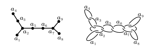
The first homology group of is given by the cokernel (over ) of the linking matrix:
| (220) |
In what follows we assume for simplicity that is a rational homology sphere (), which implies that has no loops (i.e. it is a tree). The linking form on is then given by
| (221) |
Different plumbing graphs can give homeomorphic 3-manifolds — iff and can be connected by a sequence of 3d Kirby moves, as shown in Figure 6424242There is also a move which relates a connected graph to a disconected one. For the sake of brevity we don’t discuss the case of disconnected plumbing graphs here..
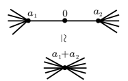
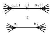
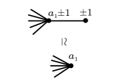
The theory can in principle be obtained by combining together the following 3d theories (see e.g. [66]):
-
•
edge: -duality wall in super-Yang-Mills (i.e. theory ),
-
•
2-valent vertex: -duality wall “supesymmetric Chern-Simons term at level ,”
-
•
-valent vertex: = copies of gauged together.
3.4.1 Homological blocks
The homological blocks can be calculated by the following formula (see appendix A for a derivation):
| (222) |
where is the degree of a vertex and, as before, “v.p.” means taking principle value integral (i.e. take half-sum of contours “dodging” poles from both sides) and is the theta function of the lattice corresponding to minus the linking form given by
| (223) |
Remarks on (222) :
-
1.
In the special case when the plumbing graph has just one vertex, the expression for the homological block reduces to (137) with .
-
2.
Generically it is well-defined only if is negative definite, i.e. is a link of a normal singularity, with being a resolution graph of the singularity.
-
3.
The formula (222) defines homological blocks in terms of a plumbing graph , but one can show that they are invariant under Kirby moves (Figure 6) acting on . Therefore, actually depends only on the homeomorphism class of , and is indeed a topological invariant. A priori this is not obvious, since (222) has been obtained (see Appendix A) as an analytic continuation of WRT invariant, which, in principle, does not have to be unique.
-
4.
Even though the formula has the structure of the “index of a quiver theory”, it is not clear how to properly realize it as a partition function of on with some boundary condition.
-
5.
Suppose . Then is a well-defined series in convergent in the unit disk . Unless is a Lens space, does not admit analytic continuation (in the usual sense) outside of due to Fabry gap theorem (because the powers of with non-zero coefficients grow quadratically).
- 6.
Example 1:
![[Uncaptioned image]](/html/1701.06567/assets/x11.png) |
(230) |
| (231) |
| (232) |
Example 2:
| (233) |
| (234) |
| (235) |
Example 3:
(non-Seifert)
![[Uncaptioned image]](/html/1701.06567/assets/x14.png) |
(236) |
| (237) |
| (238) |
3.4.2 Problems on the side
One may wish to carry out the categorification program for as well. However, it is not obvious how to write a correct expression for superconformal or topologically twisted index of the 3d theory because the UV description with supersymmetry of its certain components (see the paragraph above Section 3.4.1) is not known. In particular, there is no known Lagrangian description for half-BPS T-duality walls in super-Yang-Mills theory, and understanding the theory and its Hilbert space poses a challenge. We hope to study this problem in the future.
Let us note that a certain expression of the superconformal index of , with being an -mapping class torus of punctured (which, without a puncture, would be homeomorphic to with circular plumbing ) was considered in [74, 75]. In particular, there it was checked that it was invariant under the first two of the Kirby moves in Figure 6 that correspond to relations in the group. However, as it was argued in [75] it coincides with the result given by triangulation decomposition, as in [76, 77], and therefore, if interpreted as the partition function of the complex Chern-Simons theory, it misses contributions of the reducible flat connections [67]. The latter as we have seen, play a major role for categorification of WRT invariant. Also, in principle one can extend their prescription for calculating superconformal indices associated with plumbing graphs with vertices of degree other than two, by requiring invariance under the third Kirby move in Figure 6.
4 Adding knots and links into
The goal of this section is to incorporate knots and links in a non-trivial 3-manifold and produce the corresponding homological invariants. In particular, it will give us the very first examples where both knots and 3-manifolds are non-trivial.
The physical setup that we use to make concrete predictions for the new homological invariants was already briefly mentioned in (69). As before, denotes a knot in while denotes a representation (color) of CS gauge group . The case of links is similar and involves assigment of color to each component of the link. The space can be explored from a number of vantage points and in a variety of duality frames (all of which lead to the same result). In particular, from the vantage point of the theory on fivebrane world-volume, incorporating knots and links corresponds to introducing a 1d defect (“impurity”) which preserves the same supersymmetry as the background along in our previous discussion, cf. Figure 1.
Alternatively, starting from the brane system (14), there are many possibilities [44] to accommodate knots inside . We focus on those which give rise to line operators in .434343The other options lead to a 3d “space-time filling defect,” deforming the theory to a new one . They correspond to codimension-four defects in the 6d (2,0) theory, engineered by either M2- or M5-branes (see e.g. [78] for a discussion in the context of 3d-3d correspondence). For example, one can insert a stack of M2-branes in the following way:
| (239) |
We have chosen the line defect in to sit at the tip (also the Taub-NUT center) to preserve the rotational symmetry. Naively, the way the stack of M2-branes ends on fivebranes is determined by a partition of the number of M2 branes into . Such partitions are in one-to-one correspondence with Young tableaux with at most rows, which are in turn can be identified with irreducible representations of . In the case of we have to mod out configurations where M2 branes are equally distributed among fivebranes. This leads to Young tableaux with at most rows that label irreducible representations of . In reality, mapping line operators in 3d/3d correspondence and in the fivebrane setup is a delicate business and should be dealt with care.
If one wishes to use M5-branes to represent knots, then besides they would also occupy the two-dimensional co-normal bundle of inside and the cotangent space to at [15]. Both constructions, based on M2- and M5-branes, lead to Wilson loops — in fact, they are related by the Hanany-Witten type effect in M-theory or, in TQFT on , by the Fourier transform from representation basis to holonomy basis.
Using this physical setup, we compute the new homological invariants for some simple examples of non-trivial knots and 3-manifolds. In particular, we verify that suitable variants of the Conjectures 9 and 20 hold in the presence of knots and links.
4.1 Links in and line operators in
Consider a knot in colored by a representation of . As described above, it corresponds to a certain half-BPS line operator in :
| (240) |
where is the category of BPS line operators in SCFT . The homological invariant for a combined system of a knot and a 3-manifold is then given by the BPS Hilbert space of on the disk with inserted at , the center of the disk (see Figure 1):
| (241) |
where denotes the choice of boundary condition, the same as in the case without a knot. It has the same gradings as before, namely the -grading and the homological (R-charge) grading :
| (242) |
And, as before, the graded Euler characteristic gives the partition function on :
| (243) |
now, in 3d theory with an extra 1d “impurity” supported on . The analogue of the Conjecture 9 is then the following:
Conjecture 4.1
The WRT invariant of with a knot colored by representation can be decomposed into the following form:
| (244) |
where
| (245) |
convergent in and is the same as in Conjecture 9
For certain 3-manifolds with an extra symmetry, preserved by the knot , we have an extra grading whose value we denote by :
| (246) |
In practice, to compute these homological invariants, one needs a convenient ultra-violet (UV) description of the fivebrane setup (239) or, better yet, of the IR superconformal theory . In general, the brane system (239) and the 3d theory may admit many such UV descriptions, in various duality frames, all of which flow to the same IR physics and produce the same homological invariants (space of BPS states).
In a given UV gauge theory description of , the objects in the tensor category of BPS line operators can be understood as vector spaces — the “Hilbert spaces of quantum mechanics on the line, coupled to the bulk gauge theory”. The most familiar line operators are Wilson operators , labeled by a representation of the UV gauge group444444In general, is different from . For a quiver theory, it may be given by a product over the vertices. (which, in general, has little to do with ). The corresponding object of the category is, tautologically, the representation . The Wilson lines are expected to form a complete basis of line operators in the IR theory, in the sense that any line operator (not necessarily associate to a knot) should have the following decomposition:
| (247) | |||||
The reason is very simple — one can always decompose the “defect Hilbert space” into representations of , with the multiplicity space associated with the representation . The symmetry plays the role of the flavor symmetry in QM on the line, which couples to 3d theory by gauging in the bulk. If is a generic physical line operator (cf. superposition of physical line operators), the corresponding multiplicity spaces are honest vector space that are at least doubly-graded, with the -grading coming from symmetry of the brane system (239). When the flavor symmetry is a symmetry of both and , the third -grading is also present.
As a trivial example, consider a line defect given by a quantum mechanics that is completely decoupled from the bulk. Then,
| (248) |
where is the Hilbert space of the quantum mechanics and is the trivial Wilson loop. So, we see that (247) has a chance of being correct, even if there are infinitely many possibilities of engineering defects via 1d-3d coupled systems. In this sense, is analogous to the label “” of the homological blocks, which reduces infinitely many possible boundary conditions to a finite set. In fact, this isn’t just an analogy — it comes from the equivalence of two categories
| (249) |
Namely, a line operator can be viewed as the interface between two boundary conditions, and picking a “reference boundary condition” (e.g. the one giving with zero brane charge) will identify the two categories. This equivalence is a special feature of 3d quantum field theories, which associate categories to , with the objects that can be interpreted either as line operators or as boundary conditions at spatial infinity.
At this point, can still be an arbitrary representation of the UV gauge group , and one might naively think that is
| (250) |
given by the representation category of . But in light of the equivalence (249), we expect to be much smaller, since is generated by finitely many simple objects (boundary conditions that give homological blocks), as we have seen in all our examples.
Indeed, (250) is often redundant, due to presence of Chern-Simons couplings in . There is a set of “integrable representations” of giving a complete basis of in , and every Wilson loop labeled by a non-integrable representation can be decomposed as
| (251) |
All such relations generate an ideal (in the categorical sense) of , and is given by the quotient
| (252) |
As a vector space, is the same as , but the algebra structure depends on and is determined by the theory in a non-trivial way. Both and depend on the duality frame (presentation of ), but it is expected that the quotient category is a topological invariant of . It describes line operators / boundary conditions in the IR theory, which is what usually meant by .
We expect, for arbitrary , the independent Wilson loops in the theory are labeled by elements in454545So far, we have ignored the difference between and the Langlands dual group because the quantities considered so far are not sensitive to the global structure of the group. However, the spectrum of Wilson loops is sensitive to this difference, and (253) is stated for the adjoint form . If has a center, one needs to add the representations of where the center acts non-trivially. Reader interested in this subject may consult [69] where this issue was extensively discussed in a similar brane system.
| (253) |
where is the root lattice of and is the Weyl group (not to be confused with Wilson line in UV description of ). The argument for this statement parallels our discussion of boundary conditions given by M2-brane charges “”, which take values in exactly the same set. And the fundamental Wilson loops are expected to come from knots wrapping torsion 1-cycles, colored by a representation of (i.e. ).
If is abelian, then is a group and one can introduce an action of line operators on boundary conditions, which we call the shift action in what follows. This action is expected because Wilson line operators , can be engineered using M2-branes464646i.e. when torsion homology class of -cable of is given by as in (239), and the label “” for homological blocks also measures M2-brane charges. In other words, a Wilson loop relates two Hilbert spaces
| (254) |
One does not a priori know whether this is an isomorphism or not, or how the gradings on the two sides are related. However, in various examples below we observe that, at the level of homological blocks , Wilson loop acts as a simple shift operator, even for if the Weyl group action is properly taken into account.
As before, our main tools for probing the new homological invariants are SUSY-protected quantities. In particular, using a UV descriptions of and a half-BPS impurity , one can compute the partition function of on with inserted along as follows:
| (255) |
where stands for the gauge fugacities of the UV gauge group and is the character of the -representation .
Similarly, we can consider the superconformal index with half-BPS impurities inserted at one (or both) poles of . The UV localization formula for the index is modified as follows (when the impurity is at the north pole):
| (256) |
As we demonstrate in a variety of examples, it obeys the modified factorization formula
| (257) |
Note, all of the above relations depend only on the IR data, namely on and its color , not on the UV description of . In particular, note that is always summed over in these relations, which goes back to the basic relation between IR line operators (“impurities”) and their description (247) in the UV theory via .
The reader should keep in mind that there are two non-trivial maps (dualities) involved in the study of knots.474747This aspect is a surprising exception to the rule that knot homology is easier than 3-manifold homology. First, there is a rather non-trivial map (247) between line operators in the IR theory and its UV description (or, rather, one of many UV descriptions). This UV/IR map has nothing to do with applications to low-dimensional topology and is a standard phenomenon in quantum field theory. In addition, there is a map between knots and links colored by in a TQFT on and half-BPS line operators (“impurities”) in the 3d theory . This map is a chapter in the so-called 3d/3d correspondence. The reason one should pay attention to both of these maps is that it is their composition which relates homological invariants of to concrete calculations in ,
Because each of these maps can be rather non-trivial, one should not confuse the representation that labels half-BPS line operators in the UV description with the “color” of . The latter is denoted by and, whenever non-trivial, leads to the -colored link homology [79, 43] in our setup (239).
So far, the discussion in this section is very general and, as such, may be somewhat abstract. We will now give some very concrete examples for .
4.2 Links in and Rozansky’s proposal
For , the theory is a particular case of (197) with and , that is the theory of 3d vector multiplet with gauge group . In this case and the only independent Wilson loop in is the trivial Wilson loop. Also, there is only one homological block . Therefore, for an arbitrary representation of , the decomposition (251) allows to write the Wilson loop as (248):
| (258) |
In other words, in this case we expect a factorization
| (259) |
where the first factor on the right-hand side is the analogue of the Khovanov-Rozansky homology of the corresponding link colored by . What is ? And, what is ?
As we shall see below, already in this relatively simple case of the map between colored knots and links in and the UV line operators in is rather non-trivial. Since Wilson loops in come from M2-branes wrapping the circle of , we expect that the precise dictionary maps to a certain link in that winds around , and the total winding number (counted with multiplicities given by ) is equal to . Regarding as a special case of the Hopf fibration (namely, the trivial fibration), in the rest of this section we present evidence for the following identification484848Note, in the unrefined / decategorified setting, is simply the unknot colored by . Although this is no longer the case in homological world, there is still a close relation between “cabling” and “color” [80, 81].
| (260) |
Specifically, corresponds to a link made of copies of the unknot along the Hopf fiber, all colored by the fundamental representation of . And for general is a linear combination of ’s that replicates the decomposition of into ’s. Such decomposition is usually referred to as the “cabling formula” (see Appendix B).
Curiously, a similar problem was already considered by Rozansky from a purely mathematical point of view in [82]. Specifically, the Conjecture 6.10 in [82] gives a concrete description for the homological invariant of the link . We shall verify that Rozansky’s proposal494949The Conjecture 6.10 in [82] contains a typo in the description of the ideal . Namely, (261) should be replaced by (262) matches exactly with the quantum field theory computation if the generators and are assigned flavor charges , that is
| (263) |
Using the decomposition of tensor products of representations, we can write the expectation value of Wilson loops in as a sum over expectation values of Wilson loops labeled by irreducible representations. Only even representations with highest weight appear in this decomposition:
| (264) |
The expectation value of the Wilson loop in , which gives the graded Euler characteristic of ,505050In this normalization, we have (265) enabling us to directly extract the information about the space .
| (266) |
can be computed using (255), with now being the 3d super-Yang-Mills theory. We obtain
| (267) |
and the expectation values of all vanish.
On the other hand, as a vector space, the homological invariant proposed in Conjecture 6.10 of [82] admits a similar decomposition into subspaces of pure -degree515151This decomposition doesn’t respect the ring structure as each subspace is not closed under multiplication.
| (268) |
Here, is a quotient of the vector space spanned by monomials of , with degree , by the relations
| (269) |
It is easy to check that525252Basically, there are non-vanishing degree monomials, and they are subject to independent relations, obtained by multiplying with degree monomials.
| (270) |
are exactly the coefficients in (264). In particular, with is empty, and the dimension of is given by the -th Catalan number. Then
| (271) |
where we have used the -degree of the generators,
| (272) | ||||
| (273) | ||||
| (274) |
If we shift the overall -degree of by units to remove the factor in (271), what remains is in perfect agreement with the expectation value of Wilson loops in 3d theory :
| (275) |
with a typical relation between and [43]:
| (276) |
So, we have verified the conjecture by Rozansky at the level of equivariant Euler characteristics for this link ,
| (277) |
presenting some evidence for the isomorphism between and with .
As a side remark, positivity also features in the invariants of three manifolds with knots, in a way similar to the case without knot (164). For example, in our case of ,
| (278) |
has only positive coefficients.
4.3 Links in
For , or more generally , we have and the basic Wilson loops in are given by with .535353Notice that we have added odd representations according to description in footnote 45. These correspond to the “-cablings” of the unknot (260) wrapping the Hopf fiber of .
More generally, for plumbed (see section 3.4), if is a -cabling of the unknot wrapping the “Hopf fiber” associated with the node of the plumbing graph, we have , where is the representation of obtained from the representation of via the “evaluation homomorphism” for the node .
4.3.1 Unrefined index of with Wilson loops
The unrefined superconformal index — with contribution of the Cartan component of the adjoint chiral removed, as in (117) — with the Wilson line inserted at the north pole reads:
| (279) | ||||
Assuming is irreducible, we identify it with its highest weight in . Our convention is such that
| (280) |
So, the insertion of an operator with odd value of automatically gives zero, because of the non-trivial action of the center .
In the table below we present explicit results for up to :
0
3
2
4
0
6
8
10
12
14
0
16
18
20
22
24
0
26
28
30
32
34
0
36
38
.
This table is almost periodic. This can be understood from the action of Wilson lines on the homological blocks.
For the partition function of with inserted at the center of the disk, , we have:
| (281) |
Wilson loops act in a very simple way on the homological blocks . For , we have
| (282) |
with the rest of the blocks being zero. Let us also formally extend for outside the range by and define a “shift operator”
| (283) |
Then,
| (284) |
This equation is not cyclic, and we took to live in . Then, one can verify that
| (285) |
One can also deduce the action of on by applying the -transform, but it won’t be very illuminating because will be a linear combination of all ’s. This difference between and again demonstrates the advantage of working with the homological blocks , rather than .
4.3.2 Refinement and categorification
The refined version of (281) reads
| (286) |
One can show that it has the positivity property (164) and, therefore, can be interpreted as the Poincaré polynomial of the homological invariant that categorifies WRT invariants of with knots wrapping the Hopf fiber.
For example, consider . With our choice of , it has three abelian flat connections and, correspondingly, three homological blocks, all tabulated in [27, sec.6]. Now, we can see that incorporating knots does not spoil the positivity of (286) and its interpretation as the Poincaré polynomial. Yet, the presence of the knot changes all homological blocks in a non-trivial way, mixing homological invariants of the knot and the ambient 3-manifold in one combined entity, e.g. for and :
| (287) |
| (288) |
and
| (289) |
Note that, when , we have and the unknot wrapping the Hopf fiber becomes the familiar unknot in , yet with a nontrivial framing equal to 1. Since , as in section 4.2, we expect factorization in this case:
| (290) |
| (291) |
Moreover, as in section 4.2, we expect that is the cabling of the unknot determined by . In appendix B, we present evidence for this by comparing it with the ordinary Khovanov homology of the cabling of the unknot, cf. [80].
4.4 Comparison with refined CS
In this section, we wish to compare the categorification of WRT invariants of knots in 3-manifolds considered in the previous section with analogous calculations using the tools of refined CS theory and DAHA [19, 72]. To the best of our knowledge, such calculations (that involve both knots and 3-manifolds) were not done in the literature on refined Chern-Simons theory.
Let us consider the unknot wrapping the Hopf fiber in and colored by an irreducible representation . Note, that now the representation (whose weight we denote by the same letter) does represent the “color” of . The partition function of the refined CS theory with such insertion can be expressed through and matrices (listed in section 3.2.6) as follows:
| (292) |
where is the Macdonald polynomial, whose coefficients are rational functions of and . By repeating the manipulations of section 3.2.6, we obtain (up to the same simple overall factor):
| (293) |
with
| (294) |
For , the Macdonald polynomial coincides with the Schur polynomial, , and the expression above agrees with the partition function with a Wilson line insertion (286). However, in order to find an agreement for more general , we need to make a replacement in (286). At the catogorified level, this means that (260) needs to be replaced by
| (295) |
where are appropriate categorifications of the coefificients in the decomposition . This suggests that the insertion of the Macdonald polynomial in the partition function of 3d theory corresponds to a -colored unknot wrapping the Hopf fiber of , cf. (260):
| (296) |
It would be interesting to test this against many examples of -colored homology for various knots and links [79, 72, 43, 83, 44, 84, 85].
Note, that the coefficients in fusion rules of Macdonald polynomials are non-trivial rational functions of . Therefore, the dependence on in (294) does not agrees with the cabling formula, unlike the case of Wilson line insertions. On the other hand, the dependence on framing in the refined CS is simple and is given by the corresponding power of the matrix element . In particular, when the result of (294) is
| (297) |
Note that, for , it is a nontrivial rational function of and , which means that the underlying doubly graded vector space is infinite dimensional, unlike the finite dimensional vector spaces produced by Wilson line insertions (see Appendix B).
Acknowledgments.
We would like to thank J. E. Andersen, M. Aganagic, F. Benini, C. Cordova, A. Gadde, E. Gorsky, K. Hori, H. Kim, S. Nawata, M. Romo, S. Shakirov, L. Rozansky and K. Ye for useful comments and discussions. The work of S.G. and D.P. is supported in part by the U.S. Department of Energy, Office of Science, Office of High Energy Physics, under Award Number DE-SC0011632. In addition, the work of D.P. is supported by the center of excellence grant “Center for Quantum Geometry of Moduli Space” from the Danish National Research Foundation (DNRF95). P.P. gratefully acknowledges the support from Marvin L. Goldberger Fellowship and the DOE Grant DE-SC0009988. The research of C.V. is supported in part by NSF grant PHY-1067976. This work was performed in part (by P.P.) at Aspen Center for Physics which is supported by National Science Foundation grant PHY-1066293. The authors would like to thank Simons Center for Geometry and Physics and the organisers of the Simons Summer Workshop 2016, where the work on the project has begun, for generous hospitality.Appendix A -valued invariant for negative definite plumbed 3-manifolds
We are interested in obtaining a certain analytic continuation of WRT invariant [86, 87] of a plumbed 3-manidfold ,545454Everything below in principle can be generalized to and . where is a tree. Let us first consider the case of positive integer level, with . The colored Jones polynomial of link is explicitly known (see e.g. [87])555555We use the normalization in which the colored Jones polynomial of unlink with components with canonical framing is given by (298) :
| (299) |
where .565656In this appendix, we use to denote a -th () root of unity and reserve to denote the corresponding continuous variable which will appear in analytic continuation. For the purposes of computing the WRT invariant of 3-manifold obtained by Dehn surgery on a link , it is useful to consider the following quantity:
| (300) |
Then the WRT invariant of is given by [86]575757Normalized such that (301)
| (302) |
where are the number of positive/negative eigenvalues of the linking matrix while denotes a plumbing graph with one vertex corresponding to an unknot with framing. The CS partition function, in the usual physical normalization, with
| (303) |
differs from (302) by a simple factor:
| (304) |
| (305) |
where , is the standard pairing on and is the signature of the linking matrix . In particular, from this formula it follows that
| (306) |
Therefore
| (307) |
where we used invariance of the summand under and the fact that . The prime ′ in the sum means that the singular values are omitted.
Consider the following factor in the expression above:
| (308) |
If one picks a vertex and makes a change , a term in the sum with a given configuration of signs associated to edges (that is ) will transform into a term with a different configuration times . Using the fact that the graph is a tree, by a sequence of such transforms, any configuration of signs can be brought to the configuration with all signs . Therefore (307) can be rewritten as follows:
| (309) |
Before we can apply (305) to (309) we need to explicitly regularize the sum. In order to do this, let us introduce the following auxiliary quantities:
| (310) |
| (311) |
Then
| (312) |
where
| (313) |
with being a finite set of elements from . If, after expansion in one collects coefficients in front of powers of , the expression has the following form:
| (314) |
where
| (315) |
and
| (316) |
Note that does not depend on the choice of in (310). Formally,
| (317) |
Now let us assume that the quadratic form is negative definite, 585858In principle, this condition can be relaxed. It is only necessary that is negative on a certain subspace of .i.e. ). Then we can define the following -series, convergent for :
| (318) |
where
| (319) |
| (320) |
| (321) |
where acts as follows:
| (322) |
which is a symmetry of (318).
Using relation (312) and applying Gauss reciprocity formula (305) we arrive at the following expression for the WRT invariant:
| (323) |
Now, assume that the limit , where is defined in (318) and approaches -th primitive root of unity from inside of the unit disc , exists and moreover,
| (324) |
Then
| (325) |
We do not provide a proof of (324), and therefore (325), but believe it should be similar to the proof of the similar statement in [90]. However, even without the relation (325), the formula (318) provides an invariant of negative-definite plumbed 3-manifolds valued in -series with integer coefficients. As was already mentioned before, the resulting -series do not depend on the auxiliary choices of in (313). One can show that they are also invariant under the action of Kirby moves (see Figure 6) acting on , and therefore indeed depend only on homeomorphism class of .
The formula (318) for the homological blocks can also be rewritten as a contour integral:
| (326) |
where is the theta function of the lattice corresponding to minus the linking form :
| (327) |
and “v.p.” again means that we take principle value integral (i.e. take half-sum of contours ). Such prescription corresponds to regularization by made in (313).
Appendix B Cabling in versus color in
Here, we illustrate a delicate feature of 3d/3d correspondence that shows up at the categorical level when knots are introduced in . (The issue goes away if one looks at the problem without knots or at the decategorified level.) Namely, we compare 3d theory on to quantum group invariants of and their categorification. As explained in section 4.1 and illustrated in Figure 1, introducing knots and links in corresponds to adding a line operator (“impurity”) of a suitable type in .
A curious aspect of this correspondence is that the representation (“color”) of the line operator in most naturally maps to the cabling data of the original knot in . At the decategorified level, that data would be the same as the color of itself, but in the homological world the story is more interesting.


Since this phenomenon can be seen already in the basic case of the unknot, we illustrate it with the simplest choice of , and with framing 1. Its colored Jones polynomials can be computed via the standard cabling formula that isolates an -dimensional irreducible representation in the tensor product of 2-dimensional fundamental representations. As in [80], applying the same formula to the ordinary Khovanov homology of the -cabling (illustrated in Figure 7):
| (328) |
we find595959using KnotTheory package for Mathematica
| (329) |
where we changed in order to show explicitly the grading (by fermion number) via signs. Note that the choice of framing played an important role in this calculation. In particular, if it was trivial, the result would be very different (even at the level of total dimensions) because the cables would be just disconnected unions of unknots, instead of non-trivial links shown in Figure 7.
Now, let us compare (329) with the expectation values (286) of the Wilson line operators in 3d theory :
| (330) |
where, as in section 4.2, we made the replacement . We find perfect agreement at the level of graded spaces, where the first factor is the -grading and the second factor is the fermion number grading. The -gradings do not exactly agree (although they are somewhat correlated). This is a standard feature of the relation between colored knot homology and homology of cablings [80, 81].
The comparison between (329) and (330) clearly shows that the representation (“color”) of the Wilson line operator in appears to map to the cabling data of the original unknot in . Note, a priori neither (329) nor (330) have any direct relation to the homology of the unknot colored by representation . Indeed, -colored homology of the unknot [79, 58] should be obtained by using the categorified Jones-Wenzl projectors [91, 92] instead of the naive cabling relations (328).
Similarly, (330) may miss the mark for two reasons. First, the variable that appears in (330) keeps track of the flavor symmetry grading, not the homological (R-symmetry) grading. This issue is not a serious objection, especially in view of the “homological-flavor locking” that allowed to identify these two gradings in many examples in this paper. A more serious issue with (330) has to do with a non-trivial map of line operators in 3d/3d correspondence. In particular, the -th cabling606060more precisely, the linear combination of cablings up to -th, given by (328) of a knot and its -colored version may be indistinguishable at the decategorified level, but they are completely different operators in the physical setup (239) and, in general, have different homological invariants (spaces of BPS states).
Appendix C Categorification of the Turaev-Viro invariants
The aim of this paper is to introduce and study new three-manifold invariants. Along the way, we have seen the important roles played by boundary conditions, abelian flat connections, homological blocks, refinement, and line operators. Here, we outline how these ideas can be applied to categorification of the Turaev-Viro invariants.
Defined via a state-sum model, the Turaev-Viro (TV) invariants [93] involve a “counting” problem from the start. This motivates a series of questions: do TV invariants of have a natural home in physics? Could it be that they are counting BPS states associated with the theory and can be categorified in a way similar to the WRT invariant? How are they related to the new invariants discussed in this paper? Can they also be decomposed into the “atoms” of three-manifold invariants — the homological blocks and abelian connections? Can they be refined?
From the perspective of the state-sum model, categorification of the Turaev-Viro invariants may potentially seem even more natural than that of Chern-Simons (WRT) invariants, though the two problems are closely connected. Thus, the TV invariant of a closed 3-manifold is simply the square of the corresponding WRT/CS invariants [94, 95, 96]:
| (331) |
As explained in detail in this paper, the WRT invariants can be written as a linear sum of homological blocks and, when there is only one block,
| (332) |
is exactly given by the index of the theory . So, for homological spheres, we have already categorified their TV invariants!
For general , the story will be more interesting.616161To streamline the presentation, we will ignore normalization factors, Weyl group actions, etc. If we use to denote the vector space of boundary conditions on of the theory (a de-categorification of ), then there are two natural bases and corresponding to the homological blocks and (connected components of) abelian flat connections. There are several distinct elements in , one is — the boundary condition at the origin of , and another is — the boundary condition at that is used to reproduce the WRT invariant. Partition function of the theory on defines the inner product on and a map . Then we have626262To obtain homological invariants, one just needs to decompactify the time circle, and will be come the category that the 3d theory associates to . Then the homological invariants are identified with between two boundary conditions , in .
| (333) | |||||
| (334) | |||||
| (335) | |||||
| (336) |
and also, in the unrefined limit,
| (337) |
Using
| (338) |
we have
| (339) |
where
| (340) |
is the shift operator that acts on by
| (341) |
with
| (342) |
being the modular transform of . The shift operators are the S-dual of Wilson loops, whose action on the homological block for , as we have seen in section 4.3.1, is
| (343) |
The S-duality of type IIB string theory becomes 3d mirror symmetry of that exchanges Wilson loops and vortex loops (see e.g. [97] for a detailed description of the map in a very large class of 3d theories), and one expects that corresponds to the insertion of a vortex line. Similar to a Wilson loop, which carries an electric charge, a vortex loop carries a magnetic flux, creating a holonomy along its meridian — no surprise that it will shift which is characterized by holonomies. The relation between vortex loops and abelian flat connections can be understood more precisely using the M-theory geometry, as we now explain.
Vortex loops come from codimension-two defects in 6d (2,0) theory and can be engineered by a stacks of “defect M5-branes” as follows:
| (344) |
where is the cotangent space at . The defect fivebranes have a flat background 2-form connection (“gerbe connection”) on its world volume. The vortex lines will carry fluxes, labeled by elements in . Analogous to the BPS state counting analysis with M2-branes, the non-torsion part of results in -exact deformations of the system, enabling us to consider only the torsion part . Taking into account multiple fivebranes gives . In other words, non-trivial BPS vortex loop are labeled by components of abelian flat connections. For M2-branes propagating in this system (344), this generates the above mentioned shift action of vortex loops on flat connections.
We have now identified the system relevant for the Turaev-Viro invariant: on with the insertion of a exotic defect, given by a linear combination of vortex loops,636363This defect can be viewed as the S-dual of a Wilson loop labeled by a reducible representation, but it will be interesting to find an alternative way to characterize this defect. whose BPS Hilbert space should categorify the TV invariant. This Hilbert space will be doubly-graded for generic and at least triply-graded for Seifert . In the latter case, we will have refinement for both TV invariants and the “TV homologies.” It would be interesting to test this proposal in concrete examples, which we leave for future work.
References
- [1] P. Kronheimer and T. Mrowka, Monopoles and three-manifolds, vol. 10. Cambridge University Press, 2007.
- [2] A. Floer, An instanton-invariant for -manifolds, Comm. Math. Phys. 118 (1988) 215–240.
- [3] P. Ozsváth and Z. Szabó, Holomorphic disks and topological invariants for closed three-manifolds, Annals of Mathematics (2004) 1027–1158.
- [4] E. Witten, Quantum Field Theory and the Jones Polynomial, Commun. Math. Phys. 121 (1989) 351–399.
- [5] N. Reshetikhin and V. G. Turaev, Invariants of -manifolds via link polynomials and quantum groups, Invent. Math. 103 (1991) 547–597.
- [6] D. Birmingham, M. Blau, M. Rakowski and G. Thompson, Topological field theory, Phys. Rept. 209 (1991) 129–340.
- [7] L. Rozansky and H. Saleur, S and T matrices for the superU(1,1) WZW model: Application to surgery and three manifolds invariants based on the Alexander-Conway polynomial, Nucl. Phys. B389 (1993) 365–423, [hep-th/9203069].
- [8] D. Chang, I. Phillips and L. Rozansky, R matrix approach to quantum superalgebras su-q(m/n), J. Math. Phys. 33 (1992) 3710–3715, [hep-th/9207075].
- [9] L. Rozansky and H. Saleur, Reidemeister torsion, the Alexander polynomial and U(1,1) Chern-Simons Theory, J. Geom. Phys. 13 (1994) 105–123, [hep-th/9209073].
- [10] G. Meng and C. H. Taubes, Sw= milnor torsion, Mathematical Research Letters 3 (1996) 661–674.
- [11] L. Crane and I. B. Frenkel, Four-dimensional topological quantum field theory, Hopf categories, and the canonical bases, J. Math. Phys. 35 (1994) 5136–5154.
- [12] M. Khovanov, A categorification of the jones polynomial, arXiv preprint math.QA/9908171 (1999) .
- [13] M. Khovanov and L. Rozansky, Matrix factorizations and link homology, Fundamenta Mathematicae 199 (2008) 1–91.
- [14] I. Frenkel, C. Stroppel and J. Sussan, Categorifying fractional Euler characteristics, Jones-Wenzl projectors and -symbols, Quantum Topol. 3 (2012) 181–253.
- [15] H. Ooguri and C. Vafa, Knot invariants and topological strings, Nucl. Phys. B577 (2000) 419–438, [hep-th/9912123].
- [16] S. Gukov, A. S. Schwarz and C. Vafa, Khovanov-Rozansky homology and topological strings, Lett. Math. Phys. 74 (2005) 53–74, [hep-th/0412243].
- [17] S. Gukov, Gauge theory and knot homologies, Fortsch. Phys. 55 (2007) 473–490, [0706.2369].
- [18] E. Witten, Fivebranes and Knots, 1101.3216.
- [19] M. Aganagic and S. Shakirov, Knot Homology and Refined Chern-Simons Index, Commun. Math. Phys. 333 (2015) 187–228, [1105.5117].
- [20] S. Chun, S. Gukov and D. Roggenkamp, Junctions of surface operators and categorification of quantum groups, 1507.06318.
- [21] S. Nawata and A. Oblomkov, Lectures on knot homology, 2015. 1510.01795.
- [22] S. Gukov, M. Marino and P. Putrov, Resurgence in complex Chern-Simons theory, 1605.07615.
- [23] S. Cecotti and C. Vafa, Topological antitopological fusion, Nucl. Phys. B367 (1991) 359–461.
- [24] S. Pasquetti, Factorisation of N = 2 Theories on the Squashed 3-Sphere, JHEP 04 (2012) 120, [1111.6905].
- [25] C. Beem, T. Dimofte and S. Pasquetti, Holomorphic Blocks in Three Dimensions, JHEP 12 (2014) 177, [1211.1986].
- [26] S. Cecotti, D. Gaiotto and C. Vafa, geometry in 3 and 4 dimensions, JHEP 05 (2014) 055, [1312.1008].
- [27] S. Gukov, P. Putrov and C. Vafa, Fivebranes and 3-manifold homology, 1602.05302.
- [28] K. Hikami, Decomposition of witten-reshetikhin-turaev invariant: linking pairing and modular forms, Chern-Simons Gauge Theory 20 (2011) 131–151.
- [29] M. Atiyah, On framings of 3-manifolds, Topology 29 (1990) 1–7.
- [30] Y. Yoshida and K. Sugiyama, Localization of 3d Supersymmetric Theories on , 1409.6713.
- [31] D. Pei and K. Ye, A 3d-3d appetizer, JHEP 11 (2016) 008, [1503.04809].
- [32] T. Dimofte, S. Gukov and L. Hollands, Vortex Counting and Lagrangian 3-manifolds, Lett. Math. Phys. 98 (2011) 225–287, [1006.0977].
- [33] M. Blau and G. Thompson, Aspects of topological gauge theories and D-branes, Nucl.Phys. B492 (1997) 545–590, [hep-th/9612143].
- [34] M. Blau and G. Thompson, Euclidean SYM theories by time reduction and special holonomy manifolds, Phys.Lett. B415 (1997) 242–252, [hep-th/9706225].
- [35] K. Hori, A. Iqbal and C. Vafa, D-branes and mirror symmetry, hep-th/0005247.
- [36] A. Haydys, Fukaya-Seidel category and gauge theory, J. Sympl. Geom. 13 (2015) 151–207, [1010.2353].
- [37] S. Cautis and J. Kamnitzer, Knot homology via derived categories of coherent sheaves. I. The -case, Duke Math. J. 142 (2008) 511–588.
- [38] P. Seidel and I. Smith, A link invariant from the symplectic geometry of nilpotent slices, Duke Math. J. 134 (2006) 453–514.
- [39] C. Manolescu, Link homology theories from symplectic geometry, Adv. Math. 211 (2007) 363–416.
- [40] M. Abouzaid and I. Smith, Khovanov homology from Floer cohomology, 1504.01230.
- [41] S. Cautis, Rigidity in higher representation theory, 1409.0827.
- [42] M. Mackaay and B. Webster, Categorified skew Howe duality and comparison of knot homologies, 1502.06011.
- [43] H. Awata, S. Gukov, P. Sulkowski and H. Fuji, Volume Conjecture: Refined and Categorified, Adv. Theor. Math. Phys. 16 (2012) 1669–1777, [1203.2182].
- [44] S. Gukov, S. Nawata, I. Saberi, M. Stošić and P. Sułkowski, Sequencing BPS Spectra, JHEP 03 (2016) 004, [1512.07883].
- [45] A. Beliakova, C. Blanchet and T. T. Q. Le, Laplace transform and universal sl(2) invariants, math/0509394.
- [46] A. Beliakova, C. Blanchet and T. T. Q. Le, Unified quantum invariants and their refinements for homology 3-spheres with 2-torsion, Fund. Math. 201 (2008) 217–239.
- [47] J. Ellegaard Andersen and R. Kashaev, A TQFT from Quantum Teichmüller Theory, Commun. Math. Phys. 330 (2014) 887–934, [1109.6295].
- [48] J. Ellegaard Andersen and R. Kashaev, A new formulation of the Teichmüller TQFT, 1305.4291.
- [49] J. E. Andersen and R. Kashaev, Faddeev’s Quantum Dilogarithm and State-Integrals on Shaped Triangulations, in Proceedings, Winter School in Mathematical Physics: Mathematical Aspects of Quantum Field Theory: Les Houches, France, January 29-February 3, 2012, pp. 131–152, Springer, Springer, 2015. DOI.
- [50] S. Garoufalidis and R. Kashaev, From state integrals to q-series, 1304.2705.
- [51] S. Garoufalidis, The 3D index of an ideal triangulation and angle structures, Ramanujan J. 40 (2016) 573–604.
- [52] S. Garoufalidis, C. D. Hodgson, J. H. Rubinstein and H. Segerman, 1-efficient triangulations and the index of a cusped hyperbolic 3-manifold, 1303.5278.
- [53] S. Garoufalidis, C. Hodgson, N. Hoffman and H. Rubinstein, The 3D-index and normal surfaces, 1604.02688.
- [54] S. Gukov and D. Pei, Equivariant Verlinde formula from fivebranes and vortices, 1501.01310.
- [55] M. Blau and G. Thompson, Chern-Simons Theory with Complex Gauge Group on Seifert Fibred 3-Manifolds, 1603.01149.
- [56] F. Benini and A. Zaffaroni, A topologically twisted index for three-dimensional supersymmetric theories, JHEP 07 (2015) 127, [1504.03698].
- [57] J. M. F. Labastida, M. Marino and C. Vafa, Knots, links and branes at large N, JHEP 11 (2000) 007, [hep-th/0010102].
- [58] E. Gorsky, S. Gukov and M. Stosic, Quadruply-graded colored homology of knots, 1304.3481.
- [59] M. Aganagic, T. Ekholm, L. Ng and C. Vafa, Topological Strings, D-Model, and Knot Contact Homology, Adv. Theor. Math. Phys. 18 (2014) 827–956, [1304.5778].
- [60] V. Shende, D. Treumann and E. Zaslow, Legendrian knots and constructible sheaves, 1402.0490.
- [61] V. Shende, D. Treumann, H. Williams and E. Zaslow, Cluster varieties from Legendrian knots, 1512.08942.
- [62] D. Jafferis and X. Yin, A Duality Appetizer, 1103.5700.
- [63] A. Kapustin, H. Kim and J. Park, Dualities for 3d Theories with Tensor Matter, JHEP 12 (2011) 087, [1110.2547].
- [64] C. Beem, M. Lemos, P. Liendo, W. Peelaers, L. Rastelli and B. C. van Rees, Infinite Chiral Symmetry in Four Dimensions, Commun. Math. Phys. 336 (2015) 1359–1433, [1312.5344].
- [65] M. Dedushenko, S. S. Pufu and R. Yacoby, A one-dimensional theory for Higgs branch operators, 1610.00740.
- [66] A. Gadde, S. Gukov and P. Putrov, Fivebranes and 4-manifolds, 1306.4320.
- [67] H.-J. Chung, T. Dimofte, S. Gukov and P. Sułkowski, 3d-3d Correspondence Revisited, JHEP 04 (2016) 140, [1405.3663].
- [68] Y. Imamura and S. Yokoyama, Index for three dimensional superconformal field theories with general R-charge assignments, JHEP 04 (2011) 007, [1101.0557].
- [69] S. Gukov, D. Pei, W. Yan and K. Ye, Equivariant Verlinde algebra from superconformal index and Argyres-Seiberg duality, 1605.06528.
- [70] J. E. Andersen, S. Gukov and D. Pei, The Verlinde formula for Higgs bundles, 1608.01761.
- [71] D. Halpern-Leistner, The equivariant Verlinde formula on the moduli of Higgs bundles, ArXiv e-prints (Aug., 2016) , [1608.01754].
- [72] I. Cherednik, Jones polynomials of torus knots via DAHA, Int.Math.Res.Not. 23 (2013) 5366–5425, [1111.6195].
- [73] F. Benini, Y. Tachikawa and D. Xie, Mirrors of 3d Sicilian theories, JHEP 09 (2010) 063, [1007.0992].
- [74] D. Gang, E. Koh and K. Lee, Superconformal Index with Duality Domain Wall, JHEP 10 (2012) 187, [1205.0069].
- [75] D. Gang, E. Koh, S. Lee and J. Park, Superconformal Index and 3d-3d Correspondence for Mapping Cylinder/Torus, JHEP 01 (2014) 063, [1305.0937].
- [76] T. Dimofte, D. Gaiotto and S. Gukov, Gauge Theories Labelled by Three-Manifolds, Commun. Math. Phys. 325 (2014) 367–419, [1108.4389].
- [77] T. Dimofte, D. Gaiotto and S. Gukov, 3-Manifolds and 3d Indices, Adv. Theor. Math. Phys. 17 (2013) 975–1076, [1112.5179].
- [78] D. Gang, N. Kim, M. Romo and M. Yamazaki, Taming supersymmetric defects in 3d–3d correspondence, J. Phys. A49 (2016) 30LT02, [1510.03884].
- [79] S. Gukov and M. Stosic, Homological Algebra of Knots and BPS States, Proc. Symp. Pure Math. 85 (2012) 125–172, [1112.0030].
- [80] M. Khovanov, Categorifications of the colored jones polynomial, Journal of Knot Theory and Its Ramifications 14 (2005) 111–130.
- [81] S. Gukov and J. Walcher, Matrix factorizations and Kauffman homology, hep-th/0512298.
- [82] L. Rozansky, A categorification of the stable su (2) witten-reshetikhin-turaev invariant of links in s2 x s1, arXiv preprint arXiv:1011.1958 (2010) .
- [83] H. Itoyama, A. Mironov, A. Morozov and A. Morozov, HOMFLY and superpolynomials for figure eight knot in all symmetric and antisymmetric representations, JHEP 07 (2012) 131, [1203.5978].
- [84] P. Wedrich, Exponential growth of colored HOMFLY-PT homology, 1602.02769.
- [85] Ya. Kononov and A. Morozov, Rectangular superpolynomials for the figure-eight knot, 1609.00143.
- [86] N. Reshetikhin and V. G. Turaev, Invariants of 3-manifolds via link polynomials and quantum groups, Inventiones mathematicae 103 (1991) 547–597.
- [87] E. Witten, Quantum field theory and the jones polynomial, Communications in Mathematical Physics 121 (1989) 351–399.
- [88] F. Deloup and V. Turaev, On reciprocity, Journal of Pure and Applied Algebra 208 (2007) 153–158.
- [89] L. C. Jeffrey, Chern-simons-witten invariants of lens spaces and torus bundles, and the semiclassical approximation, Communications in mathematical physics 147 (1992) 563–604.
- [90] R. Lawrence and D. Zagier, Modular forms and quantum invariants of 3-manifolds, Asian Journal of Mathematics 3 (1999) 93–108.
- [91] B. Cooper and V. Krushkal, Categorification of the Jones-Wenzl projectors, Quantum Topol. 3 (2012) 139–180.
- [92] B. Cooper, M. Hogancamp and V. Krushkal, homology of graphs and links, Algebr. Geom. Topol. 11 (2011) 2137–2166.
- [93] V. Turaev and O. Viro, State sum invariants of 3-manifolds and quantum 6j-symbols, Topology 31 (1992) 865 – 902.
- [94] V. G. Turaev et al., Shadow links and face models of statistical mechanics, J. Differential Geom 36 (1992) 35–74.
- [95] K. Walker, On witten’s 3-manifold invariants, preprint (1991) .
- [96] V.-G. Turaev, Quantum invariants of knots and 3-manifolds. Walter de Gruyter &Co., 1994.
- [97] B. Assel and J. Gomis, Mirror Symmetry And Loop Operators, JHEP 11 (2015) 055, [1506.01718].