Coherent coupled qubits for quantum annealing

Abstract

Quantum annealing is an optimization technique which potentially leverages quantum tunneling to enhance computational performance. Existing quantum annealers use superconducting flux qubits with short coherence times, limited primarily by the use of large persistent currents $I_{\mathrm{p}}$. Here, we examine an alternative approach, using qubits with smaller $I_{\mathrm{p}}$ and longer coherence times. We demonstrate tunable coupling, a basic building block for quantum annealing, between two flux qubits with small ($\sim 50~{}\mathrm{nA}$) persistent currents. Furthermore, we characterize qubit coherence as a function of coupler setting and investigate the effect of flux noise in the coupler loop on qubit coherence. Our results provide insight into the available design space for next-generation quantum annealers with improved coherence.

I Introduction

Quantum annealing Finnila et al. (1994); Kadowaki and Nishimori (1998); Brooke et al. (1999); Farhi et al. (2001) is a heuristic technique for finding the low energy configurations of complicated Ising models. It has received considerable interest as a potential new computing paradigm for solving classical optimization problems Lucas (2014), which are important for a wide range of applications in science and industry. Existing quantum annealers, despite rapid progress in system size and intensive efforts to benchmark performance, have yet to demonstrate improved scaling over classical methods Rønnow et al. (2014); Boixo et al. (2014); Lanting et al. (2014); Albash et al. (2015); Katzgraber et al. (2015); Isakov et al. (2015); Boixo et al. (2016); Denchev et al. (2016); Mandrà et al. (2016). While continued efforts to scale and improve existing quantum annealing architectures will provide a clearer picture of their potential capabilities, it is also worthwhile to consider their limitations and explore alternative approaches which may be more amenable to quantum-enhanced performance.

Commercial quantum annealers, developed by D-Wave Systems, are based on niobium flux qubits with relatively short coherence times and are designed to implement stoquastic Hamiltonians Bravyi et al. (2008) with pairwise Ising couplings limited to a “Chimera” connectivity graph Harris et al. (2010); Bunyk et al. (2014). Experience with the D-Wave platform suggests that it could benefit from higher connectivity, increased precision in setting parameters, and greater control over the annealing schedule. In addition, increased qubit coherence, non-stoquastic Hamiltonians, and multi-qubit interactions Kafri et al. (2017) may also be instrumental in achieving quantum-enhanced performance. In this work, we focus on the challenge of improving the coherence of coupled qubits in a quantum annealer.

Superconducting flux qubits Mooij et al. (1999); Orlando et al. (1999) are well-suited to quantum annealing, because they can be used to approximately realize the transverse Ising model Hamiltonian $\hat{H}_{I}=\tfrac{\hbar}{2}\sum_{i}(\epsilon_{i}\hat{\sigma}^{\mathrm{z}}_{i}+\Delta_{i}\hat{\sigma}^{\mathrm{x}}_{i})+\sum_{i<j}\hbar J_{ij}\hat{\sigma}^{\mathrm{z}}_{i}\hat{\sigma}^{\mathrm{z}}_{j}$, where $\hbar\epsilon_{i}$ and $\hbar\Delta_{i}$ play the roles of the Zeeman energies due to the $z$ and $x$ components of the local field seen by the $i^{\textrm{th}}$ spin, and $J_{ij}$ is the Ising interaction between spins $i$ and $j$. Here, the two eigenstates of the Pauli operator $\hat{\sigma}^{z}_{i}$ correspond to “persistent current” states of qubit $i$, which can be viewed as clockwise and counter-clockwise currents of magnitude $I_{\mathrm{p}}$ circulating around the qubit loop. For a quantum annealing device based on the Transverse Ising model, the parameters $\epsilon_{i}$ and $J_{ij}$ are used to encode a classical problem, while nonzero $\Delta_{i}$ are the source of the quantum fluctuations which drive the annealing process. In general, all of these parameters must be tunable. In a flux qubit-based implementation, a coupler mediates an interaction between qubits $i$ and $j$, and the parameters $\epsilon_{i}$, $\Delta_{i}$, and $J_{ij}$ are tunable via local magnetic flux biases.

The coupler elements Mooij et al. (1999); Plourde et al. (2004); van den Brink et al. (2005); Niskanen et al. (2006); van der Ploeg et al. (2007); Zakosarenko et al. (2007); Harris et al. (2007); Ashhab et al. (2008); Harris et al. (2009); Kafri et al. (2017); Allman et al. (2010, 2014); Chen et al. (2014) are themselves also flux qubits, though operated in a regime where they can be described as a simple flux-tunable effective inductance $L_{\text{eff}}$. In this language, the coupling energy between two qubits, each with persistent current $I_{\mathrm{p}}$ and mutual inductance $M$ with the coupler, is given by $J=I_{\mathrm{p}}^{2}M^{2}/L_{\mathrm{eff}}$. The quantity $1/L_{\mathrm{eff}}$ is also referred to as the coupler susceptibility Harris et al. (2009).

The most significant design parameter to affect the coherence of a quantum annealer is the choice of $I_{\mathrm{p}}$. Flux qubits with large persistent current have a naturally strong coupling, as $J\propto I_{\mathrm{p}}^{2}$, but their coherence times are severely limited by flux noise: their sensitivity to flux noise is proportional to $I_{\mathrm{p}}$ and can limit both the energy relaxation time and the dephasing time Yan et al. (2016); Quintana et al. (2017), which for $1/f$ flux noise roughly scale as $1/I_{\mathrm{p}}^{2}$ and $1/I_{\mathrm{p}}$, respectively. In the D-Wave system, the qubits are designed with large persistent currents $I_{\mathrm{p}}\sim 3$ $\mu$A Harris et al. (2010) in order to achieve large coupling strength with modest values of coupler susceptibility and $M$. In contrast, we recently demonstrated that it is possible to produce robust, long-lived flux qubits with small persistent currents $I_{\mathrm{p}}\sim 50$ nA Yan et al. (2016). In order to realize strong coupling between qubits with small $I_{\mathrm{p}}$, it is necessary to compensate by increasing either $M$ or the coupler susceptibility. Although this approach increases the qubit’s sensitivity to flux noise in the coupler loop and requires more precise control over the coupler flux bias, it nevertheless allows for a significant improvement in qubit coherence.

In this work, we demonstrate tunable coupling between qubits with persistent currents reduced by nearly two orders of magnitude compared to existing quantum annealers. While coupled flux qubits with low persistent currents have been previously demonstrated van der Ploeg et al. (2007), no work to date has investigated the implications that this design choice has on qubit coherence for quantum annealing. We present, for the first time, a systematic study of the coherence of coupled flux qubits in the context of quantum annealing. In particular, we investigate the effect of flux noise in the coupler loop on qubit coherence. Our results are in good agreement with simulations based on the full Hamiltonian of the coupled qubit system, as well as a semi-classical model. This work serves as a proof-of-principle and provides a framework for evaluating coherence in future quantum annealing architectures.

II Experimental setup

A circuit diagram of our coupled qubit device is shown in Figure 1a. Two capacitively shunted three-junction flux qubits, Qubit A and Qubit B, are each galvanically coupled to an rf-SQUID coupler via a shared inductance of $M=34$ pH, as shown in Figures 1b-d. The devices are controlled by the externally applied magnetic fluxes $\Phi_{\mathrm{A}}$, $\Phi_{\mathrm{B}}$, and $\Phi_{\mathrm{C}}$. For simplicity, our experiments use qubits with a single superconducting loop, instead of the multi-loop qubits that are required for independent $\Delta$ tunability. We characterize the qubits using standard dispersive measurements Blais et al. (2004), with each qubit coupled to a separate readout resonator which is probed through a shared transmission line.

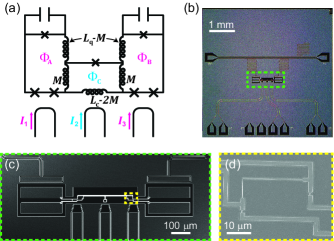
Figure 1: Coupled qubit geometry. (a) Device schematic. Qubit A (left loop) and Qubit B (right loop) are capacitively shunted three-junction flux qubits, coupled through a shared inductance with an rf-SQUID coupler (center loop). On-chip bias currents $I_{1}$, $I_{2}$, and $I_{3}$ control the external fluxes $\Phi_{\mathrm{A}}$, $\Phi_{\mathrm{C}}$, and $\Phi_{\mathrm{B}}$ through the qubit and coupler loops. (b) Optical micrograph of the aluminum (light grey) device on a silicon (dark grey) substrate. (c) Optical image showing the qubits, coupler, and flux bias lines. (d) SEM image of the galvanic connection between Qubit B (lower-right) and the coupler (upper-left).

The transition frequency between the coupler ground- and first-excited state $\omega_{\mathrm{C}}^{\mathrm{01}}/2\pi$ was designed to be $\sim 20$ GHz, which is significantly larger than the qubit transition frequencies at $\sim 5$ GHz. Therefore, the coupled qubit system can be described by the approximate low-energy Hamiltonian $H\approx H_{\mathrm{q}}^{(\mathrm{A})}+H_{\mathrm{q}}^{(\mathrm{B})}+H_{\mathrm{int}}$ Harris et al. (2007), where

$$H_{\mathrm{q}}^{(i)}=\frac{\hbar}{2}[\epsilon_{i}(\Phi_{\mathrm{A,B,C}})\hat{\sigma}_{\mathrm{z}}^{(i)}+\Delta_{i}(\Phi_{\mathrm{A,B,C}})\hat{\sigma}_{\mathrm{x}}^{(i)}],$$ (1)

$$H_{\mathrm{int}}=\hbar J(\Phi_{\mathrm{A,B,C}})\sigma_{\mathrm{z}}^{(\mathrm{A})}\sigma_{z}^{(\mathrm{B})}.$$ (2)

The effective parameters $\epsilon_{i}$, $\Delta_{i}$, and $J$ are not only determined by the circuit parameters of the individual qubits and coupler, but also by their couplings, and can depend on all three flux biases. For each qubit, the degeneracy point is defined as the bias where $\epsilon_{i}=0$. A table of device parameters can be found in Appendix A.

The qubits were designed with shunt capacitance $C_{\mathrm{sh}}=50$ fF, loop inductance $L_{\mathrm{q}}=110$ pH, and $I_{\mathrm{p}}=45$ nA. All device components were patterned from a high-quality evaporated aluminum film on a high-resistivity silicon wafer, except for the superconducting loops and Josephson junctions, which were deposited using double-angle evaporation of aluminum Yan et al. (2016). Spectroscopy plots showing the energy difference between the ground and first excited state for Qubit A and Qubit B are shown in Figures 2a,b as a function of the reduced flux $f_{\mathrm{i}}\equiv\Phi_{\mathrm{i}}/\Phi_{0}$ in the qubit loop, with the coupler biased at $f_{\mathrm{C}}=0$. At this coupler bias, $\Delta_{\mathrm{A}}/2\pi=5.042$ GHz and $\Delta_{\mathrm{B}}/2\pi=5.145$ GHz.

Figure 2: Qubit spectroscopy. Dashed black traces: semi-classical model. Solid green traces: simulations of the full circuit Hamiltonian. (a) Spectroscopy of Qubit A vs $f_{A}$, with $f_{B}=f_{C}=0$. (b) Spectroscopy of Qubit B vs $f_{\mathrm{B}}$ with $f_{\mathrm{A}}=f_{\mathrm{C}}=0$. The yellow dashed line represents the starting point and range of qubit frequencies in the following panel. (c) Spectroscopy of Qubit B vs $f_{\mathrm{C}}$ for $f_{\mathrm{A}}=0$ and $f_{\mathrm{B}}=0.516$. The regions of anti-ferromagnetic (AF), ferromagnetic (FM), and zero coupling are indicated. The inset shows detailed data for the FM region.

Figure 2c shows how the transition frequency of Qubit B depends on the coupler bias. This dependence originates from the circulating current in the coupler loop $\langle I^{\mathrm{C}}\rangle$, which couples to the qubit through the shared inductance $M$. Thus, the coupler induces an offset flux in the qubit loop, which shifts the effective qubit bias as indicated by the dashed line in Figure 2b. Treating the interaction classically, the offset flux is given by $\delta f_{\mathrm{B}}=M\langle I^{\mathrm{C}}\rangle/\Phi_{0}$. Assuming that the coupler remains in its ground state, $\langle I^{\mathrm{C}}\rangle$ and $L_{\text{eff}}$ are related to the coupler ground state energy $E_{0}^{(\mathrm{C})}$ as

$$\langle I^{\mathrm{C}}\rangle\equiv\frac{\partial E_{0}^{(\mathrm{C})}}{\partial\Phi_{\mathrm{C}}};\frac{1}{L_{\mathrm{eff}}}\equiv\frac{\partial\langle I^{\mathrm{C}}\rangle}{\partial\Phi_{\mathrm{C}}}=\frac{\partial^{2}E_{0}^{(\mathrm{C})}}{\partial\Phi_{\mathrm{C}}^{2}}.$$ (3)

By fitting our results to theory we extract the rf-SQUID coupler loop inductance $L_{\mathrm{C}}=470$ pH and junction critical current $I_{\mathrm{C}}^{0}=730$ nA, giving $\beta\equiv 2\pi L_{\mathrm{C}}I_{\mathrm{C}}^{0}/\Phi_{0}$ = 1.04. $\langle I^{\mathrm{C}}\rangle$ and $1/L_{\text{eff}}$ vary with $f_{C}$, and for these coupler parameters they range from -700 to 700 nA and $1/(1070~{}\mathrm{pH})$ to $1/(-48~{}\mathrm{pH})$, respectively. Note that the slope of $\langle I^{\mathrm{C}}\rangle$ with respect to flux determines the sign of $L_{\mathrm{eff}}$ and, thus, the sign of $J$. Therefore, Figure 2c can be seen as a map of the regions of anti-ferromagnetic ($J>0$), ferromagnetic ($J<0$), and zero coupling.

III Coupling strength

Two-qubit coupling is shown in Figure 3, focusing primarily on the ferromagnetic coupling regime. Panels (a-f) show spectroscopy of both qubits as the transition frequency of Qubit A is tuned through resonance with that of Qubit B, which is held at a fixed bias. When the qubits are resonant their levels hybridize and split in frequency by $2|J|$, shown here for three coupler biases corresponding to different values of coupling strength $J$. Panel (g) shows the qubit frequencies for maximal coupling, as $f_{\mathrm{A}}$ is tuned over a much larger range. At this coupler bias, we measure a maximal coupling strength of $|J|/2\pi=94$ MHz. From this measurement and our experimental bound on the minimum coupling (see Appendix E), we place a lower bound of $425$ on the coupler on/off ratio. Finally, panel (h) shows the dependence of $|J|$ on the coupler bias, which agrees well with simulations of the full circuit Hamiltonian, as well as a semi-classical model (see Appendix B).

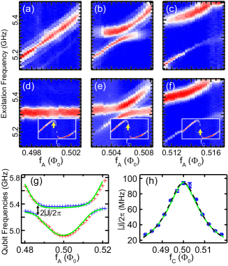
Figure 3: Qubit-qubit coupling. Dashed black traces: semi-classical model. Solid green traces: simulations of the full circuit Hamiltonian. (a-f) Spectroscopy of qubit level crossings for different coupling strengths. Panels (a-c) and (d-f) show measurements using Resonator A and Resonator B, respectively. In each panel we scan $f_{A}$ while holding $f_{B}$ at a fixed bias point $\sim 10~{}\mathrm{m}\Phi_{0}$ away from degeneracy. The left, middle, and right panels correspond to zero ($f_{\mathrm{C}}=0.402$), intermediate ($f_{\mathrm{C}}=0.48$), and maximum ($f_{\mathrm{C}}=0.5$) coupling, as indicated by the insets. (g) Avoided level crossings as Qubit A (red) is tuned across Qubit B (blue) with $f_{\mathrm{C}}=0.5$. (h) J vs coupler bias. Error bars are derived from the error of fitting the qubit spectroscopy to a double Gaussian function.

IV Qubit coherence

In Figure 4, we show how the properties of an individual qubit depend on the coupler bias. Here, we present data for Qubit B, with $f_{\mathrm{A}}$ set to zero. Panels (a,b) display $\Delta_{\mathrm{B}}$ versus $f_{\mathrm{C}}$. For each value of $f_{\mathrm{C}}$, we sweep $f_{\mathrm{B}}$ and perform qubit spectroscopy to find the minimum qubit frequency, $\omega_{\mathrm{B}}^{\mathrm{min}}(f_{\mathrm{C}})\equiv\Delta_{\mathrm{B}}(f_{\mathrm{C}})$. The dependence of $\Delta_{\mathrm{B}}$ on $f_{\mathrm{C}}$ can be understood semi-classically as loading of the qubit inductance by the effective inductance of the coupler,

$$L_{\mathrm{q}}^{\mathrm{loaded}}=L_{\mathrm{q}}-\frac{M^{2}}{L_{\mathrm{eff}}},$$ (4)

as illustrated by the dashed lines in Figures 4a,b.

In Figures 4c,d we show how the qubit energy relaxation time $T_{1}$ depends on $f_{\mathrm{C}}$. For each coupler bias point, Qubit B is biased on degeneracy (at the point of minimum qubit frequency). Error bars correspond to the standard error for fitting the decay curve at each coupler bias point to an exponential function. In addition to any dependence on the coupler bias, $T_{1}$ also fluctuates on slow timescales Yan et al. (2016); Gustavsson et al. (2016), and the grey band indicates the typical range of $T_{1}$ fluctuations when the coupler is biased away from degeneracy (see Appendix D). When the coupler is biased near degeneracy, we observe a reduction in $T_{1}$ substantially below the range of temporal fluctuations.

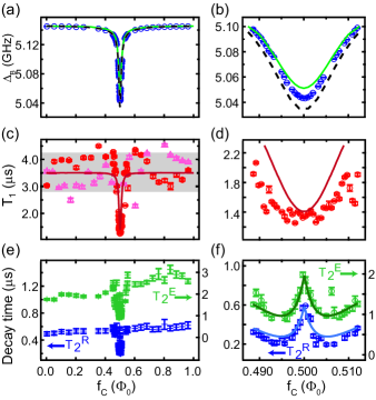
Figure 4: Qubit properties vs coupler bias. Results for Qubit B, with $f_{\mathrm{A}}=0$. Left column: full range of coupler biases. Right column: zoom in near coupler degeneracy. (a,b) $\Delta_{\mathrm{B}}$ vs coupler bias. Dashed black traces: semi-classical model. Solid green traces: simulations of the full circuit Hamiltonian. (c,d) Qubit energy relaxation time vs coupler bias. The red circles and the magenta triangles correspond to measurements taken at different times. The grey band indicates the typical range of $T_{1}$ variations when the coupler is biased away from degeneracy. The solid line represents an upper bound on qubit $T_{1}$ due to flux noise in the coupler loop with an exponent $\alpha=0.91$ and an amplitude of $15~{}\mu\Phi_{0}/\sqrt{\mathrm{Hz}}$, combined in parallel with a coupler-independent relaxation time of $3.5~{}\mu$s. (e,f) Ramsey (left axis) and echo (right axis) $1/e$ decay times vs coupler bias. Solid lines show the expected dependence due to $1/f^{\alpha}$ flux noise in the coupler loop with the same amplitude and exponent as above.

Finally, panels (e,f) show the dependence of the qubit dephasing times on $f_{\mathrm{C}}$, for the same bias conditions as above. Here, we report the $1/e$ decay times $T_{2}^{\mathrm{Ramsey}}$ and $T_{2}^{\mathrm{Echo}}$ for Ramsey interferometry and spin echo experiments, respectively. When the coupler is biased away from degeneracy, $T_{2}^{\mathrm{Ramsey}}$ is essentially constant with respect to $f_{\mathrm{C}}$. There is some variation in $T_{2}^{\mathrm{Echo}}$, which is roughly consistent with the range of values expected from the observed fluctuations in $T_{1}$.

Interestingly, we observe a sharp reduction in the coherence times as the coupler bias approaches degeneracy, and a full recovery when the coupler is biased exactly on degeneracy. This effect can be understood as the result of the first-order sensitivity of $\Delta_{\mathrm{B}}$ to the coupler bias, which is given by $\partial\Delta_{\mathrm{B}}/\partial\Phi_{\mathrm{C}}$, the slope of the data in panels (a,b). By fitting the measured dependence of $\Delta_{\mathrm{B}}$ on $f_{\mathrm{C}}$ and assuming a $1/f^{\alpha}$ spectral density of fluctuations with $\alpha=0.91$ , we see excellent agreement between our model and the coherence measurements for a flux noise amplitude of $15$ $\mu\Phi_{0}/\sqrt{\text{Hz}}$, as indicated by the curves in Figure 4f. Using the same amplitude and exponent, we calculate an upper limit on qubit $T_{1}$ due to flux noise in the coupler loop, as shown in Figure 4c,d. In Appendix D, we speculate on why the estimated flux noise amplitude is larger than previously reported values for flux qubits made with the same fabrication process Yan et al. (2016) and the potential implications for future quantum annealing architectures designed to optimize for both coherence and coupling.

This work represents an important step toward designing quantum annealers with improved coherence. We have demonstrated tunable coupling between flux qubits with substantially lower persistent currents than existing commercial devices, thereby reducing the qubit sensitivity to flux noise in their respective loops. This approach requires an increased coupler susceptibility, which increases the qubits’ sensitivity to flux noise in the coupler loop. We have examined this effect by measuring qubit coherence across the full range of coupler biases, using standard measurement techniques borrowed from the gate-based quantum computing community, which have yet to be applied to commercial quantum annealers. Looking forward, our approach can be extended to achieve larger coupling strength, symmetric bipolar coupling, and $\hat{\sigma}_{\mathrm{x}}\hat{\sigma}_{\mathrm{x}}$ interactions Kerman and Oliver (2008), while maintaining low persistent currents. Our results provide new insights into the available design space and suggest the type of systems-level analysis that will be necessary when designing quantum annealers with improved coherence.

	Parameter	Semi-classical model	Full galvanic circuit model
Common junction params.	$J_{\mathrm{c}}$ ($\mu$A)	2.78	2.78
	$S_{\mathrm{c}}$ (fF/$\mu\mathrm{m}^{2}$)	50	50
Qubit A	$I_{\mathrm{0}}^{\mathrm{A,sm}}(\mathrm{nA})$	78	78
	$I_{\mathrm{0}}^{\mathrm{A,lg}}(\mathrm{nA})$	206	206
	$C_{\mathrm{sh}}^{\mathrm{A}}$ (fF)	53	53
	$L_{\mathrm{q}}^{\mathrm{A}}$ (pH)	115	115
Qubit B	$I_{\mathrm{0}}^{\mathrm{B,sm}}(\mathrm{nA})$	78	78
	$I_{\mathrm{0}}^{\mathrm{B,lg}}(\mathrm{nA})$	209	209
	$C_{\mathrm{sh}}^{\mathrm{B}}$ (fF)	53	53
	$L_{\mathrm{q}}^{\mathrm{B}}$ (pH)	115	115
Coupling	$M$ (pH)	39	43
	$I_{\mathrm{0}}^{\mathrm{C}}(\mathrm{nA})$	727	736
	$L_{\mathrm{C}}$ (pH)	467	542

Table 1: Table of sample parameters.

Appendix A Table of sample parameters

Table 1 shows a list of sample parameters extracted from two different models of the coupled qubit system—a semi-classical model, where the individual qubits and coupler are treated quantum mechanically but their interactions are treated as a classical mutual inductance, and a quantum model of the full galvanically-coupled circuit. Using the semi-classical model, we performed an optimization routine to determine the set of parameters which best fit the results in Figures 2-4. The quantum model includes some effects, such as cross-capacitance between the qubits and coupler, which are not included in the semi-classical model. Therefore, it was necessary to make small adjustments to the parameters extracted from the semi-classical model in order to achieve good agreement between the quantum model and the measured results, as indicated in Table 1.

Appendix B Semi-classical model

Figure 5 shows a circuit diagram for the full galvanically-coupled circuit. To simulate the energy levels of the full system, we diagonalize the circuit Hamiltonian, using similar techniques to our previous work Yan et al. (2016). These techniques are described in detail in a separate forthcoming publication .

In this section, we explain how to map the full circuit onto a simpler and more computationally convenient semi-classical model. In this model, the individual qubits and coupler are treated quantum mechanically, but their interactions are treated as a classical mutual inductance. Using this simplified model, we derive expressions for the coupling strength $J$, as well as the shifts in the qubit parameters $\Delta$ and $\epsilon$ due to interaction with the coupler.

B.1 Comparing mutually-inductive coupling to galvanic coupling

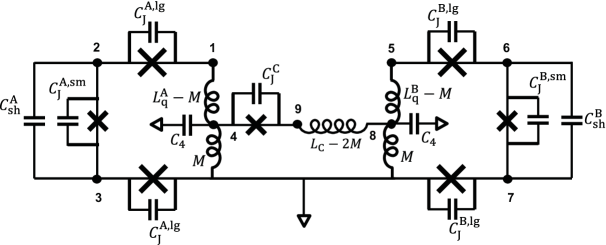
Figure 5: Schematic diagram of the full galvanic circuit. The nodes of the circuit, labeled $1-9$, are used to define its canonical flux and charge variables Devoret and Martinis (2003).

To build up the model of the coupled qubit system, we first consider a simpler system depicted in Figure 6a. Here, two loops of inductance $L_{\mathrm{A,B}}$ threaded by magnetic flux $\Phi_{\mathrm{A,B}}$ are coupled through a mutual inductance $M$.

Defining the flux vector $\bm{\Phi}$, the mutual inductance matrix $\bm{M}$, and the self-inductance matrix $\bm{L}$ as

$$\bm{\Phi}\equiv\begin{pmatrix}\Phi_{\mathrm{A}}\\ \Phi_{\mathrm{B}}\end{pmatrix};~{}\bm{M}\equiv\begin{pmatrix}0&-M\\ -M&0\end{pmatrix};~{}\bm{L}\equiv\begin{pmatrix}L_{\mathrm{A}}&0\\ 0&L_{\mathrm{B}}\end{pmatrix},$$ (5)

the classical potential energy of the system is given by

$$U =\frac{1}{2}\bm{\Phi}\left(\bm{L}^{-1}+\bm{L}^{-1}\bm{M}\bm{L}^{-1}\right)\bm{\Phi}$$ (6)

$$=\frac{1}{2}\frac{\Phi_{\mathrm{A}}^{2}}{L_{\mathrm{A}}}+\frac{1}{2}\frac{\Phi_{\mathrm{B}}^{2}}{L_{\mathrm{B}}}+M\frac{\Phi_{\mathrm{A}}}{L_{\mathrm{A}}}\frac{\Phi_{\mathrm{B}}}{L_{\mathrm{B}}},$$ (7)

where the first two terms correspond to the energies of the individual loops, and the third term represents their interaction energy. The system can be re-expressed in terms of the classical circulating currents $I_{\mathrm{A,B}}=\Phi_{\mathrm{A,B}}/L_{\mathrm{A,B}}$, which yields

$$U=\frac{1}{2}L_{\mathrm{A}}I_{\mathrm{A}}^{2}+\frac{1}{2}L_{\mathrm{B}}I_{\mathrm{B}}^{2}+MI_{\mathrm{A}}I_{\mathrm{B}}.$$ (8)

Next, we will compare this result for two mutually coupled loops to the case of two galvanically coupled loops, as depicted in Figure 6b. Here, the inductance matrix can be approximately defined as 

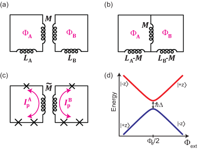
Figure 6: Direct coupling. (a) Circuit schematic for two loops of inductance $L_{\mathrm{A,B}}$ coupled through a mutual inductance $M$. (b) Circuit schematic for two loops which are galvanically coupled through a shared inductance $M$. (c) Circuit schematic for two flux qubits with persistent currents $I_{\mathrm{p}}^{\mathrm{A,B}}$ coupled through a mutual inductance $\tilde{M}$. (d) Illustration of the energies of the ground (blue) and first-excited (red) states of a flux qubit as a function of the external flux $\Phi_{\mathrm{ext}}$ through the qubit loop. At the degeneracy point ($\Phi_{\mathrm{ext}}=\Phi_{0}/2$), the ground and excited states are separated in energy by $\hbar\Delta$. When biased away from degeneracy, the qubit states are approximately persistent current states $\ket{\pm z}$.

$$\bm{L}\equiv\begin{pmatrix}L_{\mathrm{A}}&-M\\ -M&L_{\mathrm{B}}\end{pmatrix}$$ (9)

and the potential energy is given by

$$U =\frac{1}{2}\bm{\Phi}\bm{L}^{-1}\bm{\Phi}$$ (10)

$$=\frac{1}{2}\frac{\Phi_{\mathrm{A}}^{2}}{L_{\mathrm{A}}-M^{2}/L_{\mathrm{B}}}+\frac{\Phi_{\mathrm{B}}^{2}}{L_{\mathrm{B}}-M^{2}/L_{\mathrm{B}}}+M\left(1-\frac{M^{2}}{L_{\mathrm{A}}L_{\mathrm{B}}}\right)^{-1}\frac{\Phi_{\mathrm{A}}}{L_{\mathrm{A}}}\frac{\Phi_{\mathrm{B}}}{L_{\mathrm{B}}}.$$ (11)

Note that this is equivalent to equation (7) after the following substitutions:

$$\tilde{L}_{\mathrm{A,B}}\equiv L_{\mathrm{A,B}}-\frac{M^{2}}{L_{\mathrm{B,A}}};~{}\tilde{M}\equiv M\left(1-\frac{M^{2}}{L_{\mathrm{A}}L_{\mathrm{B}}}\right).$$ (12)

Thus, the galvanically-coupled circuits employed in this work can be approximately mapped onto simpler mutually-coupled circuits using the renormalized inductances $\tilde{L}$ and $\tilde{M}$.

B.2 Directly-coupled qubits

Now, suppose that each loop in the circuits discussed above is replaced with a flux qubit (FIG. 6c,d) described by the Hamiltonian $H_{\mathrm{q}}/\hbar\approx(\epsilon\hat{\sigma}_{\mathrm{z}}+\Delta\hat{\sigma}_{\mathrm{x}})/2$. In the persistent current basis, the eigenstates of the Pauli operator $\hat{\sigma}_{\mathrm{z}}$, denoted $\ket{\pm z}$, correspond to clockwise and counter-clockwise circulating currents

$$I\equiv\bra{\pm z}\hat{I}\ket{\pm z}=\bra{\pm z}I_{\mathrm{p}}\hat{\sigma}_{\mathrm{z}}\ket{\pm z}=\pm I_{\mathrm{p}},$$ (13)

where $\hat{I}$ is the current operator and $I_{\mathrm{p}}$ is magnitude of the qubit persistent current. The interaction term from equation (8) can be expressed as

$$H_{\mathrm{int}}=\tilde{M}I_{\mathrm{p}}^{\mathrm{A}}I_{\mathrm{p}}^{\mathrm{B}}\hat{\sigma}_{\mathrm{z}}^{(\mathrm{A})}\hat{\sigma}_{\mathrm{z}}^{(\mathrm{B})},$$ (14)

which takes the form $H_{\mathrm{int}}=J\hat{\sigma}_{\mathrm{z}}^{(\mathrm{A})}\hat{\sigma}_{\mathrm{z}}^{(\mathrm{B})}$, where the coupling strength $J$ is given by

$$\hbar J=\tilde{M}I_{\mathrm{p}}^{\mathrm{A}}I_{\mathrm{p}}^{\mathrm{B}}.$$ (15)

A simple intuitive picture for this expression emerges when the qubits are biased such that $\epsilon\gg\Delta$. In this regime, qubit energy eigenstates are approximately equal to the persistent current states $\ket{\pm z}$ with energy eigenvalues $\pm\hbar\epsilon/2=I_{\mathrm{p}}(\Phi_{\mathrm{ext}}-\Phi_{0}/2)$, where $\Phi_{\mathrm{ext}}$ is the external magnetic flux through the qubit loop and $\Phi_{0}$ is the magnetic flux quantum. Here, the $\hat{\sigma}_{\mathrm{z}}\hat{\sigma}_{\mathrm{z}}$ interaction is longitudinal with respect to the energy eigenbasis. The coupling can be understood by considering the effect of the persistent current in one qubit loop on the flux through the other qubit loop. For example, Qubit A induces a state-dependent offset $\delta\Phi_{\mathrm{B}}=\pm\tilde{M}I_{\mathrm{p}}^{\mathrm{A}}$ in the flux through Qubit B and thus a state-dependent frequency shift of

$$\delta\omega_{\mathrm{01}}^{(B)}\approx\pm\epsilon\delta\Phi_{\mathrm{B}}=\pm 2J.$$ (16)

Note that the coupling measurements reported in the main text were performed in the $\Delta\gg\epsilon$ regime, where the $\hat{\sigma}_{\mathrm{z}}\hat{\sigma}_{\mathrm{z}}$ interaction is transverse with respect to the energy eigenbasis. In this case, the coupling manifests as an avoided crossing between the $\ket{01}$ and $\ket{10}$ states, which are shifted from their bare energies by $\pm\hbar J$.

B.3 Mediated coupling

As a next step in building up the semi-classical coupling model, we consider the case of two qubits coupled through a mutual inductance $\tilde{M}$ to an intermediate loop of inductance $L$ (FIG. 7a). Returning to the longitudinal coupling picture ($\epsilon\gg\Delta$), the persistent current in Qubit A will induce a state-dependent offset flux $\delta\Phi_{\mathrm{C}}=\pm\tilde{M}I_{\mathrm{p}}^{\mathrm{A}}$ in the coupler loop, which changes the current circulating in the loop by $\delta\langle I^{\mathrm{C}}\rangle=\delta\Phi_{\mathrm{C}}/L$ and thus induces an offset of

$$\delta\Phi_{\mathrm{B}}=\delta\Phi_{\mathrm{C}}\frac{\tilde{M}}{L}=\frac{\tilde{M}^{2}}{L}I_{\mathrm{p}}^{\mathrm{A}}$$ (17)

in the flux through Qubit B. Note that this expression takes the same form as for the directly-coupled qubits, but with the substitution $\tilde{M}\rightarrow\tilde{M}^{2}/L\equiv M_{\mathrm{eff}}$. Then, in analogy to equation (15), the coupling strength is given by

$$J=\frac{\tilde{M}^{2}}{L}I_{\mathrm{p}}^{\mathrm{A}}I_{\mathrm{p}}^{\mathrm{B}}=M_{\mathrm{eff}}I_{\mathrm{p}}^{\mathrm{A}}I_{\mathrm{p}}^{\mathrm{B}}.$$ (18)

Finally, we consider the case where the intermediate loop is replaced with an RF-SQUID coupler (FIG. 7b). In the following discussion, we make the assumption that transition frequency between the coupler ground- and first-excited state is much larger than the qubit frequencies and that the coupler is always operated in its ground state. In general, the coupler ground state energy $E_{0}$ varies with applied flux $f_{\mathrm{C}}$, as illustrated in Figure 7c. For the coupler parameters considered in this work, the circulating current in the coupler loop is approximately equal to the slope of coupler energy with respect to flux, $\langle I^{\mathrm{C}}\rangle\approx\partial E_{0}^{\mathrm{C}}/\partial\Phi_{\mathrm{C}}$, as illustrated in Figure  7d, where we compare this quantity with the expectation value of the current operator $\bra{g}\hat{I}\ket{g}$ for the coupler ground sate $\ket{g}$.

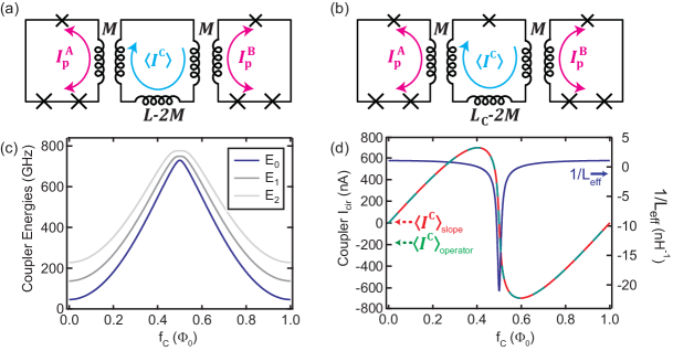
Figure 7: Mediated coupling. (a) Circuit schematic for two flux qubits with persistent currents $I_{\mathrm{p}}^{\mathrm{A,B}}$ which each couple through a mutual inductance $\tilde{M}$ to an intermediate loop of inductance $L$. (b) Circuit schematic for a similar configuration, but with the intermediate loop replaced with an RF-SQUID coupler. (c) Illustration of the energies of the ground (blue) and first-excited (grey) states of a an RF-SQUID coupler, as a function of the external flux $\Phi_{\mathrm{c}}$ through the coupler loop. (d) Left axis: comparison of the coupler circulating current, calculated using the slope of the ground state energy (red) and using and using the current operator (green). Right axis: effective inductance of the coupler vs. $\Phi_{\mathrm{c}}$.

We then define the “quantum inductance” for the coupler (as in References Johansson et al. (2006); Tornberg and Johansson (2007); Harris et al. (2009) and in analogy to the “quantum capacitance” described in the charge qubit Sillanpää et al. (2005); Duty et al. (2005); Johansson et al. (2006) and semi-conducting qubit Colless et al. (2013); Petersson et al. (2010); Ilani et al. (2006); Glazman et al. (1992); Fogler (2005); Latessa et al. (2005) literature) as

$$\frac{1}{L_{\mathrm{eff}}}\equiv\frac{\partial\langle I^{\mathrm{C}}\rangle}{\partial\Phi_{\mathrm{C}}}\approx\frac{\partial^{2}E_{0}^{(\mathrm{C})}}{\partial\Phi_{\mathrm{C}}^{2}}.$$ (19)

Note that unlike a physical inductance, this quantum inductance can take both positive and negative values. Following the same logic as above, we can now express the coupling strength as

$$J=\frac{\tilde{M}^{2}}{L_{\mathrm{eff}}}I_{\mathrm{p}}^{\mathrm{A}}I_{\mathrm{p}}^{\mathrm{B}}.$$ (20)

Given a set of qubit and coupler parameters, it is straightforward to calculate $J$ using equation (20). We determine $L_{\mathrm{eff}}$ by numerically diagonalizing the coupler Hamiltonian to solve for its ground state energy $E_{0}$ as a function of $\Phi_{\mathrm{C}}$. We separately determine $I_{\mathrm{p}}$ by numerically solving for the energy eigenstates $\ket{\psi_{j}}$ of the qubit Hamiltonian, from which we calculate the matrix elements of the current operator, $\bra{\psi_{j}}\hat{I}\ket{\psi_{k}}$, expressed in the energy eigenbasis. When the qubit is biased on degeneracy ($\epsilon=0$), the $I_{\mathrm{p}}$ is given by the off-diagonal matrix elements.

Note that equation (20) is the same expression for coupling strength used by D-Wave in references Harris et al. (2007, 2009), with the coupler susceptibility $\chi$ defined as the inverse of the effective inductance. However, their approach differs in that instead of diagnolizing the coupler Hamiltonian to solve for $\chi$, D-Wave chooses to approximate $\chi$ as the first-order (linear) susceptibility, which can be expressed using a simple analytic formula. This approach works sufficiently well for the coupler parameters of existing D-Wave devices, but the linear approximation breaks down for larger coupler susceptibilities and coupling strengths, as discussed in reference Kafri et al. (2017).

B.4 Qubit flux offset due to coupler

The semi-classical model can also explain the shifts in qubit parameters due to their interaction with the coupler. For concreteness and to follow the presentation of the main text, we will focus on Qubit B. First, we consider the effect of the coupler on the qubit flux bias. This effect explains the dependence of the qubit frequency on the coupler bias shown in Figure 2c.

As shown in Figure  7d, the circulating current in the coupler loop $\langle I^{\mathrm{C}}\rangle$ varies with the coupler bias $\Phi_{\mathrm{C}}$. This circulating current couples into the qubit loop through the mutual inductance $M$, and therefore threads a flux

$$\delta\Phi_{\mathrm{B}}=\tilde{M}\langle I^{\mathrm{C}}\rangle$$ (21)

through the qubit loop. For a flux qubit described by the Hamiltonian $H_{\mathrm{q}}/\hbar\approx(\epsilon\hat{\sigma}_{\mathrm{z}}+\Delta\hat{\sigma}_{\mathrm{x}})/2$, this flux offset corresponds to a shift in $\epsilon$ of

$$\delta\epsilon=\frac{2}{\hbar}I_{\mathrm{p}}\delta\Phi_{\mathrm{B}}=\frac{2}{\hbar}\tilde{M}I_{\mathrm{p}}\langle I^{\mathrm{C}}\rangle.$$ (22)

B.5 Inductive loading model

The coupler also affects the value of $\Delta$, the qubit frequency when biased at its degeneracy point, as shown for Qubit B in Figure 4a,b. This effect can be modeled semi-classically as inductive loading of the qubit inductance by the effective inductance of the coupler.

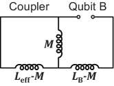
Figure 8: Inductive loading model. Circuit schematic used to model the loading of the qubit inductance due to the coupler $L_{\mathrm{eff}}$.

A circuit schematic for the inductive loading model is shown in Figure 8 . Here, we consider the impedance looking out from the Josephson junction, to calculate loaded qubit inductance

$$L_{\mathrm{B}}^{\mathrm{loaded}}=L_{\mathrm{B}}-M+\left(\frac{1}{L_{\mathrm{eff}}-M}+\frac{1}{M}\right)^{-1}=L_{\mathrm{B}}-\frac{M^{2}}{L_{\mathrm{eff}}}.$$ (23)

Note that this expression for the loaded inductance is the same as the renormalized inductance derived in equation (12). To calculate the semi-classical theory curves for $\Delta_{\mathrm{B}}$ versus $f_{\mathrm{C}}$ (FIG. 4a,b), we first simulate the coupler to determine $L_{\mathrm{eff}}(f_{\mathrm{C}})$ (FIG.  7d). Then, for each value of $f_{\mathrm{C}}$, we determine $\Delta_{\mathrm{B}}$ by simulating the qubit energy levels using $L_{\mathrm{B}}^{\mathrm{loaded}}$ for the qubit loop inductance.

Appendix C Variations of $T_{1}$ in time

In addition to any systematic dependence of $T_{1}$ on the qubit and coupler biases, we also observe $T_{1}$ variations in time. These variations are possibly related to quasiparticle fluctuations, as described in reference Gustavsson et al. (2016). Although $T_{1}$ fluctuations are not a primary focus of this work, they affect the interpretation of the data shown in Figure 4c,d. In Figure 9 we show the results of repeated $T_{1}$ measurements for Qubit B, with the coupler biased away from degeneracy. The range of observed $T_{1}$ values over the $14$ hour measurement time is represented as a grey band in Figure 4c.

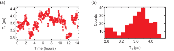
Figure 9: Repeated $T_{1}$ measurements. (a) Repeated measurements of $T_{1}$ of Qubit B as a function of time. Here, $f_{\mathrm{A}}=0$, $f_{\mathrm{B}}=0.5$, and $f_{\mathrm{C}}=0$. (b) Histogram of measured $T_{1}$ values.

Appendix D Modeling the effect of flux noise on qubit coherence

D.1 Definition of noise spectral density

In this work, as in reference Yan et al. (2016), we choose to characterize noise by the symmetric power spectral density (PSD)

$$S_{\lambda}(\omega)=\int_{-\infty}^{\infty}\mathrm{d}\tau\mathrm{exp}(-i\omega\tau)\frac{1}{2}\langle\hat{\lambda}(0)\hat{\lambda}(\tau)+\hat{\lambda}(\tau)\hat{\lambda}(0)\rangle,$$ (24)

where $\hat{\lambda}$ is an operator representing a fluctuating parameter $\lambda$. The two dominant noise mechanisms for the coupled qubit system presented here are flux noise in the qubit loop and the coupler loop, $\lambda_{i}=\Phi_{\mathrm{B}},\Phi_{\mathrm{C}}$. For $1/f$-like noise, the noise amplitude $A_{\lambda}$ is given by 

$$S_{\lambda}(\omega)=A_{\lambda}^{2}\left(\frac{2\pi\times 1\mathrm{Hz}}{\omega}\right)^{\gamma},$$ (25)

where $\gamma\sim 1$.

D.2 Energy relaxation due to $1/f^{\gamma}$-flux noise

We have analyzed the data for $T_{1}$ of our qubit-coupler system using the Fermi’s golden rule model presented in reference Yan et al. (2016),

$$\frac{1}{T_{1}}=\sum_{\lambda}2\frac{|\bra{e}\hat{D}_{\lambda}\ket{g}|^{2}}{\hbar^{2}}S_{\lambda}\left(\omega\right),$$ (26)

where the sum is taken over decay mechanisms, $S_{\lambda}\left(\omega\right)$ is the power spectral density of the noise responsible for each decay mechanism, and the operator $\hat{D}_{\lambda}$ is the transition dipole moment which couples our system to each noise source.

For the coupled system considered here, $T_{1}$ can be decomposed into contributions from the qubit, $T_{1}^{\mathrm{Q}}$, and the coupler, $T_{1}^{\mathrm{C}}$, where

$$\frac{1}{T_{1}}=\frac{1}{T_{1}^{\mathrm{Q}}}+\frac{1}{T_{1}^{\mathrm{C}}}.$$ (27)

The qubit contribution dominates away from coupler degeneracy, and both processes contribute when the system is biased near coupler degeneracy.

In our analysis, we assume that the coupler is flux noise limited on its degeneracy, and its decay rate is thus given by

$$\frac{1}{T_{1}^{\mathrm{C}}}=2\frac{|\bra{e}\hat{I}^{\mathrm{C}}\ket{g}|^{2}}{\hbar^{2}}S_{\Phi_{\mathrm{C}}}\left(\omega\right),$$ (28)

where $\ket{g}$ and $\ket{e}$ are the ground and first excited state of the coupled system

$$\hat{H}=\hat{H}^{\mathrm{Q}}+\hat{H}^{\mathrm{C}}+M\hat{I}^{\mathrm{Q}}\hat{I}^{\mathrm{C}}.$$ (29)

The quantum operators $\hat{H}^{\mathrm{C}}$ and $\hat{I}^{\mathrm{C}}$ ($\hat{H}^{\mathrm{Q}}$ and $\hat{I}^{\mathrm{Q}}$) are the Hamiltonian and loop current operator of the bare coupler (qubit) respectively, and the exact value of the matrix element $\bra{e}\hat{I}^{\mathrm{C}}\ket{g}$ can thus be calculated from the device parameters listed in Section A and the full quantum model of the bare qubit and coupler. As described in Section E, the amplitude and exponent of the flux noise power spectral density in our coupler loop are then chosen to fit the measured values of $T_{1}$, $T_{2}^{\mathrm{Ramsey}}$, and $T_{2}^{\mathrm{Echo}}$ on coupler degeneracy.

D.3 First order sensitivity to flux noise

The sensitivity $\kappa_{\lambda}$ of the qubit freqency to a parameter $\lambda$ determines the effect of fluctuations in $\lambda$ on qubit dephasing. In the two-level approximation of the flux qubit, the qubit transition frequency is given by $\omega_{\mathrm{01}}\approx\sqrt{\epsilon^{2}+\Delta^{2}}$, and, to first order,

$$\kappa_{\lambda}\equiv\frac{\partial\omega_{\mathrm{01}}}{\partial\lambda}\approx\frac{\partial\omega_{\mathrm{01}}}{\partial\epsilon}\frac{\partial\epsilon}{\partial\lambda}+\frac{\partial\omega_{\mathrm{01}}}{\partial\Delta}\frac{\partial\Delta}{\partial\lambda}=\frac{\epsilon}{\omega_{\mathrm{01}}}\kappa_{\epsilon,\lambda}+\frac{\Delta}{\omega_{\mathrm{01}}}\kappa_{\Delta,\lambda},$$ (30)

where $\kappa_{\epsilon,\lambda}\equiv\partial\epsilon/\partial\lambda$ and $\kappa_{\Delta,\lambda}\equiv\partial\Delta/\partial\lambda$.

In the measurements presented in Figure 4, we characterized the coherence of Qubit B when biased near its degeneracy point ($\epsilon_{\mathrm{B}}=0$). At this bias point, $\kappa_{\epsilon_{\mathrm{B}},\Phi_{\mathrm{B}}}$ and $\kappa_{\epsilon_{\mathrm{B}},\Phi_{\mathrm{C}}}$ are zero. Since $\Delta_{\mathrm{B}}$ depends only weakly on $\Phi_{\mathrm{B}}$, the dominant first-order noise mechanism is $\kappa_{\Delta_{\mathrm{B}},\Phi_{\mathrm{C}}}$, the sensitivity of $\Delta_{\mathrm{B}}$ to the coupler flux.

D.4 Decoherence due to $1/f^{\gamma}$-flux noise

Here, we consider the effect of $1/f$-like flux noise, as defined in equation (25), on qubit coherence. In general, this type of noise causes phase decay of the form $\mathrm{exp}[-\chi_{N}(t)]$, where Bylander et al. (2011)

$$\chi_{N}(\tau)=\frac{1}{2\pi}\tau^{2}\sum_{\lambda}\kappa_{\lambda}^{2}\int_{0}^{\infty}\mathrm{d}\omega S_{\lambda}(\omega)g_{N}(\omega,\tau),$$ (31)

where $\tau$ is the free evolution time and $g_{N}$ is a filter function which depends on the qubit pulse sequence. For the Ramsey ($N=0$) and a Hanh echo sequences ($N=1$) considered in this work,

$$g_{0}(\omega,\tau) \equiv g_{0}(\omega\tau)=\left(\frac{\mathrm{sin}(\omega\tau/2)}{(\omega\tau/2)}\right)^{2},$$ (32)

$$g_{1}(\omega,\tau) \equiv g_{1}(\omega\tau)=\left(\frac{\mathrm{sin}(\omega\tau/4)}{(\omega\tau/4)}\right)^{2}\mathrm{sin}^{2}(\omega\tau/4).$$ (33)

Substituting equation (25) into equation (31) and making the additional substitution $\omega\tau\rightarrow z$ gives

$$\chi_{N}(\tau)=\frac{(2\pi\times 1~{}\mathrm{Hz})^{\gamma}}{2\pi}\tau^{1+\gamma}\sum_{\lambda}\kappa_{\lambda}^{2}A_{\lambda}^{2}\int_{0}^{\infty}\frac{\mathrm{d}z}{z^{\gamma}}g_{N}(z),$$ (34)

where we have assumed that the fluctuations in each parameter $\lambda$ share a common noise exponent $\gamma$.

We define the $1/e$ dephasing rates $\Gamma_{N,\lambda}$, for each dephasing channel as

$$\Gamma_{N,\lambda}=\left[(2\pi)^{\gamma-1}\kappa_{\lambda}^{2}A_{\lambda}^{2}\int_{0}^{\infty}\frac{\mathrm{d}z}{z^{\gamma}}g_{N}(z)\right]^{1/(1+\gamma)}\equiv\left[\kappa_{\lambda}A_{\lambda}\eta_{N}^{1/2}\right]^{2/(1+\gamma)},$$ (35)

where the numerical factors $\eta_{0},\eta_{1}$ depend on the noise exponent $\gamma$ and the Ramsey and echo filter functions and are defined as

$$\eta_{N}=(2\pi)^{\gamma-1}\int_{0}^{\infty}\frac{\mathrm{d}z}{z^{\gamma}}g_{N}(z).$$ (36)

As discussed in Bylander et al. (2011), for the case of $\gamma=1$, these factors are given by

$$\eta_{0} \approx\mathrm{ln}\left(\frac{1}{\omega_{\mathrm{low}}t}\right)$$ (37)

$$\eta_{1} =\mathrm{ln}(2),$$ (38)

where $\omega_{\mathrm{low}}$ is the lower cutoff frequency set by the total time of all experimental iterations and $t$ is the typical free evolution time during a single experimental iteration. Note that $\eta_{1}$ is completely independent of the cutoff frequency, thus avoiding any ambiguity in choosing $\omega_{\mathrm{low}}$ and $t$ when analyzing echo experiments, while $\eta_{0}$ varies only weakly with $\omega_{\mathrm{low}}t$ for realistic measurement settings.

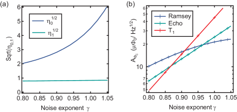
Figure 10: Flux noise analysis (a)$\sqrt{\eta_{0,1}}$ vs $\gamma$, determined through numerical integration. When calculating $\eta_{0}$, we have assumed $\omega_{\mathrm{low}}/2\pi=3~{}\mathrm{mHz}$ and $t=200~{}\mathrm{ns}$. (b) Estimated coupler flux noise amplitude based measured Ramsey, Echo, and $T_{1}$ times, as a function of $\gamma$.

For $\gamma\neq 1$, we determine the numerical factors through numerical integration of equation (36), as discussed in reference Sank et al. (2012). For the Ramsey sequence,

$$\eta_{0}=(2\pi)^{\gamma-1}\int_{\omega_{\mathrm{low}}t}^{\infty}\frac{\mathrm{d}z}{z^{\gamma}}\left(\frac{\mathrm{sin}(z/2)}{z/2}\right)^{2}$$ (39)

and for the Echo sequence,

$$\eta_{1}=(2\pi)^{\gamma-1}\int_{0}^{\infty}\frac{\mathrm{d}z}{z^{\gamma}}\left(\frac{\mathrm{sin}(z/4)}{z/4}\right)^{2}\mathrm{sin}^{2}(z/4)$$ (40)

Figure S4a shows $\sqrt{\eta_{0,1}}$ as a function of $\gamma$ for $\omega_{\mathrm{low}}/2\pi=3~{}\mathrm{mHz}$ and $\tau=200~{}\mathrm{ns}$.

D.5 Estimating the flux noise amplitude in the coupler loop

We now combine the results of the previous sections with our qubit coherence measurements to estimate the flux noise amplitude and exponent in the coupler loop. We first consider the Ramsey and Echo results presented in Figure 4e,f. We define the total $1/e$ decay rates for Ramsey and Echo experiments as $\Gamma_{\mathrm{0}}\equiv 1/T_{2}^{\mathrm{Ramsey}}$ and $\Gamma_{\mathrm{1}}\equiv 1/T_{2}^{\mathrm{Echo}}$, respectively. We separate the decay rates into two contributions: $\Gamma_{N,\mathrm{\Phi_{C}}}$ due to flux noise in the coupler loop and $\Gamma_{N,\mathrm{other}}$, which includes the effect of $T_{1}$ as well as any additional dephasing.

When the coupler is biased far from degeneracy, $\Gamma_{N,\mathrm{\Phi_{C}}}$ is negligible, and thus $\Gamma_{N}=\Gamma_{N,\mathrm{other}}$. For simplicity, we model $\Gamma_{N,\mathrm{other}}$ as exponential decay . For arbitrary coupler bias, the total phase decay takes the form

$$\mathrm{exp}[-\Gamma_{N,\mathrm{other}}\tau-(\Gamma_{N,\mathrm{\Phi_{C}}}\tau)^{1+\gamma}].$$ (41)

Thus, we can determine $\Gamma_{N,\mathrm{\Phi_{C}}}$ from the measured values of $\Gamma_{N}$ and $\Gamma_{N,\mathrm{other}}$ through the relation

$$\Gamma_{N,\mathrm{\Phi_{C}}}=\Gamma_{N}\left(1-\frac{\Gamma_{N,\mathrm{other}}}{\Gamma_{N}}\right)^{1/(1+\gamma)}$$ (42)

Finally, from equation 35 the spectral density of flux noise in the coupler is given by

$$A_{\Phi_{\mathrm{C}}}=\kappa_{\Phi_{\mathrm{C}}}^{-1}\eta_{N}^{-1/2}(\Gamma_{N,\Phi_{\mathrm{C}}})^{(1+\gamma)/2},$$ (43)

where $\kappa_{\Phi_{\mathrm{C}}}\approx\kappa_{\Delta_{B},\Phi_{\mathrm{C}}}$ is experimentally determined from the slope of $\Delta_{\mathrm{B}}$ vs $\Phi_{\mathrm{C}}$ (FIG. 4a,b).

In Figure 10b we plot the value of $A_{\Phi_{\mathrm{C}}}$ that fits best to our Ramsey and Echo measurements using equation 43, and to our $T_{1}$ measurements using equation 28, for different values of $\gamma$. Although we are unable to choose values of $A_{\Phi_{\mathrm{C}}}$ and $\gamma$ that fit perfectly with all three measurements, they are roughly bounded within the triangular region between the three curves in Figure 10b, where $10~{}\mu\Phi_{0}/\sqrt{\mathrm{Hz}}<A_{\Phi_{\mathrm{C}}}<19~{}\mu\Phi_{0}/\sqrt{\mathrm{Hz}}$ and $0.86<\gamma<0.96$. For concreteness, when plotting theory curves in the main text we choose $\gamma=0.91$ and $A_{\Phi_{\mathrm{C}}}=15~{}\mu\Phi_{0}/\sqrt{\mathrm{Hz}}$, which results in reasonably good agreement with all three measurements.

This estimate for the flux noise in the coupler loop is substantially larger than the value previously reported for flux qubits made with the same fabrication process, where we measured a flux noise amplitude of $1.4$ $\mu\Phi_{0}/\sqrt{\text{Hz}}$ Yan et al. (2016). The most significant difference between the coupler loop and the low-noise qubit loops is the loop size; the coupler loop is $20$ times larger in area. Therefore, these results motivate future efforts to study the dependence of flux noise on loop size beyond the scope of this work and previous efforts Lanting et al. (2009). Such measurements would help to inform architectural choices for optimizing coherence and coupling in next-generation quantum annealers.

Appendix E Residual coupling with coupler biased ‘off’

Here, we describe the technique that we used to place an upper bound on any residual coupling when the coupler is nominally biased to provide zero coupling ($f_{\mathrm{C}}=0.402$). As illustrated in Figure 11, we observe no avoided crossing in spectroscopy, allowing us to bound any nonzero residual coupling to $<220$ kHz, a limit determined by the resolution in $f_{\mathrm{A}}$ set by our bias current source. For each value of $f_{\mathrm{A}}$, the frequency of Qubit A is determined by fitting the spectroscopy trace to a Gaussian function. Qubit B is biased on degeneracy, and its frequency is precisely determined through Ramsey spectroscopy.

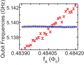
Figure 11: Zero coupling. Detailed data for the qubit level crossing with the coupler nominally biased for zero coupling ($f_{\mathrm{C}}=0.5$). Red hourglasses: Qubit A. Blue circles: Qubit B.

References

- Finnila et al. (1994) A. Finnila, M. Gomez, C. Sebenik, C. Stenson, and J. Doll, Quantum annealing: A new method for minimizing multidimensional functions, Chemical Physics Letters 219, 343 (1994).
- Kadowaki and Nishimori (1998) T. Kadowaki and H. Nishimori, Quantum annealing in the transverse ising model, Phys. Rev. E 58, 5355 (1998).
- Brooke et al. (1999) J. Brooke, D. Bitko, T. F. Rosenbaum, and G. Aeppli, Quantum annealing of a disordered magnet, Science 284, 779 (1999).
- Farhi et al. (2001) E. Farhi, J. Goldstone, S. Gutmann, J. Lapan, A. Lundgren, and D. Preda, A quantum adiabatic evolution algorithm applied to random instances of an np-complete problem, Science 292, 472 (2001).
- Lucas (2014) A. Lucas, Ising formulations of many np problems, Frontiers in Physics 2, 5 (2014).
- Rønnow et al. (2014) T. F. Rønnow, Z. Wang, J. Job, S. Boixo, S. V. Isakov, D. Wecker, J. M. Martinis, D. A. Lidar, and M. Troyer, Defining and detecting quantum speedup, Science 345, 420 (2014).
- Boixo et al. (2014) S. Boixo, T. F. Ronnow, S. V. Isakov, Z. Wang, D. Wecker, D. A. Lidar, J. M. Martinis, and M. Troyer, Evidence for quantum annealing with more than one hundred qubits, Nat Phys 10, 218 (2014).
- Lanting et al. (2014) T. Lanting, A. J. Przybysz, A. Y. Smirnov, F. M. Spedalieri, M. H. Amin, A. J. Berkley, R. Harris, F. Altomare, S. Boixo, P. Bunyk, N. Dickson, C. Enderud, J. P. Hilton, E. Hoskinson, M. W. Johnson, E. Ladizinsky, N. Ladizinsky, R. Neufeld, T. Oh, I. Perminov, C. Rich, M. C. Thom, E. Tolkacheva, S. Uchaikin, A. B. Wilson, and G. Rose, Entanglement in a quantum annealing processor, Phys. Rev. X 4, 021041 (2014).
- Albash et al. (2015) T. Albash, I. Hen, F. M. Spedalieri, and D. A. Lidar, Reexamination of the evidence for entanglement in a quantum annealer, Phys. Rev. A 92, 062328 (2015).
- Katzgraber et al. (2015) H. G. Katzgraber, F. Hamze, Z. Zhu, A. J. Ochoa, and H. Munoz-Bauza, Seeking quantum speedup through spin glasses: The good, the bad, and the ugly, Phys. Rev. X 5, 031026 (2015).
- Isakov et al. (2015) S. Isakov, I. Zintchenko, T. Rønnow, and M. Troyer, Optimised simulated annealing for ising spin glasses, Computer Physics Communications 192, 265 (2015).
- Boixo et al. (2016) S. Boixo, V. N. Smelyanskiy, A. Shabani, S. V. Isakov, M. Dykman, V. S. Denchev, M. H. Amin, A. Y. Smirnov, M. Mohseni, and H. Neven, Computational multiqubit tunnelling in programmable quantum annealers, Nature Communications 7, 10327 (2016).
- Denchev et al. (2016) V. S. Denchev, S. Boixo, S. V. Isakov, N. Ding, R. Babbush, V. Smelyanskiy, J. Martinis, and H. Neven, What is the computational value of finite-range tunneling? Phys. Rev. X 6, 031015 (2016).
- Mandrà et al. (2016) S. Mandrà, Z. Zhu, W. Wang, A. Perdomo-Ortiz, and H. G. Katzgraber, Strengths and weaknesses of weak-strong cluster problems: A detailed overview of state-of-the-art classical heuristics versus quantum approaches, Phys. Rev. A 94, 022337 (2016).
- Bravyi et al. (2008) S. Bravyi, D. P. Divincenzo, R. Oliveira, and B. M. Terhal, The complexity of stoquastic local hamiltonian problems, Quantum Info. Comput. 8, 361 (2008).
- Harris et al. (2010) R. Harris, J. Johansson, A. J. Berkley, M. W. Johnson, T. Lanting, S. Han, P. Bunyk, E. Ladizinsky, T. Oh, I. Perminov, E. Tolkacheva, S. Uchaikin, E. M. Chapple, C. Enderud, C. Rich, M. Thom, J. Wang, B. Wilson, and G. Rose, Experimental demonstration of a robust and scalable flux qubit, Phys. Rev. B 81, 134510 (2010).
- Bunyk et al. (2014) P. I. Bunyk, E. M. Hoskinson, M. W. Johnson, E. Tolkacheva, F. Altomare, A. J. Berkley, R. Harris, J. P. Hilton, T. Lanting, A. J. Przybysz, and J. Whittaker, Architectural considerations in the design of a superconducting quantum annealing processor, IEEE Transactions on Applied Superconductivity 24, 1 (2014).
- Kafri et al. (2017) D. Kafri, C. Quintana, Y. Chen, A. Shabani, J. M. Martinis, and H. Neven, Tunable inductive coupling of superconducting qubits in the strongly nonlinear regime, Phys. Rev. A 95, 052333 (2017).
- Mooij et al. (1999) J. E. Mooij, T. P. Orlando, L. Levitov, L. Tian, C. H. van der Wal, and S. Lloyd, Josephson persistent-current qubit, Science 285, 1036 (1999).
- Orlando et al. (1999) T. P. Orlando, J. E. Mooij, L. Tian, C. H. van der Wal, L. S. Levitov, S. Lloyd, and J. J. Mazo, Superconducting persistent-current qubit, Phys. Rev. B 60, 15398 (1999).
- Plourde et al. (2004) B. L. T. Plourde, J. Zhang, K. B. Whaley, F. K. Wilhelm, T. L. Robertson, T. Hime, S. Linzen, P. A. Reichardt, C.-E. Wu, and J. Clarke, Entangling flux qubits with a bipolar dynamic inductance, Phys. Rev. B 70, 140501 (2004).
- van den Brink et al. (2005) A. M. van den Brink, A. J. Berkley, and M. Yalowsky, Mediated tunable coupling of flux qubits, New Journal of Physics 7, 230 (2005).
- Niskanen et al. (2006) A. O. Niskanen, K. Harrabi, F. Yoshihara, Y. Nakamura, and J. S. Tsai, Spectroscopy of three strongly coupled flux qubits, Phys. Rev. B 74, 220503 (2006).
- van der Ploeg et al. (2007) S. H. W. van der Ploeg, A. Izmalkov, A. M. van den Brink, U. Hübner, M. Grajcar, E. Il’ichev, H.-G. Meyer, and A. M. Zagoskin, Controllable coupling of superconducting flux qubits, Phys. Rev. Lett. 98, 057004 (2007).
- Zakosarenko et al. (2007) V. Zakosarenko, N. Bondarenko, S. H. W. van der Ploeg, A. Izmalkov, S. Linzen, J. Kunert, M. Grajcar, E. Il’ichev, and H.-G. Meyer, Realization of a classical counterpart of a scalable design for adiabatic quantum computation, Applied Physics Letters 90, 022501 (2007).
- Harris et al. (2007) R. Harris, A. J. Berkley, M. W. Johnson, P. Bunyk, S. Govorkov, M. C. Thom, S. Uchaikin, A. B. Wilson, J. Chung, E. Holtham, J. D. Biamonte, A. Y. Smirnov, M. H. S. Amin, and A. Maassen van den Brink, Sign- and magnitude-tunable coupler for superconducting flux qubits, Phys. Rev. Lett. 98, 177001 (2007).
- Ashhab et al. (2008) S. Ashhab, A. O. Niskanen, K. Harrabi, Y. Nakamura, T. Picot, P. C. de Groot, C. J. P. M. Harmans, J. E. Mooij, and F. Nori, Interqubit coupling mediated by a high-excitation-energy quantum object, Phys. Rev. B 77, 014510 (2008).
- Harris et al. (2009) R. Harris, T. Lanting, A. J. Berkley, J. Johansson, M. W. Johnson, P. Bunyk, E. Ladizinsky, N. Ladizinsky, T. Oh, and S. Han, Compound josephson-junction coupler for flux qubits with minimal crosstalk, Phys. Rev. B 80, 052506 (2009).
- Allman et al. (2010) M. S. Allman, F. Altomare, J. D. Whittaker, K. Cicak, D. Li, A. Sirois, J. Strong, J. D. Teufel, and R. W. Simmonds, rf-squid-mediated coherent tunable coupling between a superconducting phase qubit and a lumped-element resonator, Phys. Rev. Lett. 104, 177004 (2010).
- Allman et al. (2014) M. S. Allman, J. D. Whittaker, M. Castellanos-Beltran, K. Cicak, F. da Silva, M. P. DeFeo, F. Lecocq, A. Sirois, J. D. Teufel, J. Aumentado, and R. W. Simmonds, Tunable resonant and nonresonant interactions between a phase qubit and resonator, Phys. Rev. Lett. 112, 123601 (2014).
- Chen et al. (2014) Y. Chen, C. Neill, P. Roushan, N. Leung, M. Fang, R. Barends, J. Kelly, B. Campbell, Z. Chen, B. Chiaro, A. Dunsworth, E. Jeffrey, A. Megrant, J. Y. Mutus, P. J. J. O’Malley, C. M. Quintana, D. Sank, A. Vainsencher, J. Wenner, T. C. White, M. R. Geller, A. N. Cleland, and J. M. Martinis, Qubit architecture with high coherence and fast tunable coupling, Phys. Rev. Lett. 113, 220502 (2014).
- Yan et al. (2016) F. Yan, S. Gustavsson, A. Kamal, J. Birenbaum, A. P. Sears, D. Hover, T. J. Gudmundsen, D. Rosenberg, G. Samach, S. Weber, J. L. Yoder, T. P. Orlando, J. Clarke, A. J. Kerman, and W. D. Oliver, The flux qubit revisited to enhance coherence and reproducibility, Nature Communications 7, 12964 (2016).
- Quintana et al. (2017) C. M. Quintana, Y. Chen, D. Sank, A. G. Petukhov, T. C. White, D. Kafri, B. Chiaro, A. Megrant, R. Barends, B. Campbell, Z. Chen, A. Dunsworth, A. G. Fowler, R. Graff, E. Jeffrey, J. Kelly, E. Lucero, J. Y. Mutus, M. Neeley, C. Neill, P. J. J. O’Malley, P. Roushan, A. Shabani, V. N. Smelyanskiy, A. Vainsencher, J. Wenner, H. Neven, and J. M. Martinis, Observation of classical-quantum crossover of flux noise and its paramagnetic temperature dependence, Phys. Rev. Lett. 118, 057702 (2017).
- Blais et al. (2004) A. Blais, R.-S. Huang, A. Wallraff, S. M. Girvin, and R. J. Schoelkopf, Cavity quantum electrodynamics for superconducting electrical circuits: An architecture for quantum computation, Phys. Rev. A 69, 062320 (2004).
- Gustavsson et al. (2016) S. Gustavsson, F. Yan, G. Catelani, J. Bylander, A. Kamal, J. Birenbaum, D. Hover, D. Rosenberg, G. Samach, A. P. Sears, S. J. Weber, J. L. Yoder, J. Clarke, A. J. Kerman, F. Yoshihara, Y. Nakamura, T. P. Orlando, and W. D. Oliver, Suppressing relaxation in superconducting qubits by quasiparticle pumping, Science (2016), 10.1126/science.aah5844.
- Note (1) In our previous work Yan et al. (2016), we determined that for capacitively shunted flux qubits with loops produced using our fabrication process. Here, we have chosen to use in order achieve a good fit to our coherence data, as discussed in Appendix D.
- Kerman and Oliver (2008) A. J. Kerman and W. D. Oliver, High-fidelity quantum operations on superconducting qubits in the presence of noise, Phys. Rev. Lett. 101, 070501 (2008).
- Note (2) A. J. Kerman, in preparation.
- Devoret and Martinis (2003) M. H. Devoret and J. M. Martinis, in Quantum Entanglement and Information Processing (Les Houches Session LXXIX), edited by J.-M. Raimond, J. Dalibard, and D. Esteve (Elsevier, New York, 2003) pp. 443–485.
- Note (3) This 2x2 inductance matrix is appropriate in the limit of small island capacitance of the node connecting the three inductors; In this limit, independent phase fluctuations of this node can be neglected, and the circuit can be described by only two canonical phase variables with a 2x2 inductance matrix.
- Johansson et al. (2006) G. Johansson, L. Tornberg, and C. M. Wilson, Fast quantum limited readout of a superconducting qubit using a slow oscillator, Phys. Rev. B 74, 100504 (2006).
- Tornberg and Johansson (2007) L. Tornberg and G. Johansson, Dispersive charge and flux qubit readout as a quantum measurement process, Journal of Low Temperature Physics 146, 227 (2007).
- Sillanpää et al. (2005) M. A. Sillanpää, T. Lehtinen, A. Paila, Y. Makhlin, L. Roschier, and P. J. Hakonen, Direct observation of josephson capacitance, Phys. Rev. Lett. 95, 206806 (2005).
- Duty et al. (2005) T. Duty, G. Johansson, K. Bladh, D. Gunnarsson, C. Wilson, and P. Delsing, Observation of quantum capacitance in the cooper-pair transistor, Phys. Rev. Lett. 95, 206807 (2005).
- Colless et al. (2013) J. I. Colless, A. C. Mahoney, J. M. Hornibrook, A. C. Doherty, H. Lu, A. C. Gossard, and D. J. Reilly, Dispersive readout of a few-electron double quantum dot with fast rf gate sensors, Phys. Rev. Lett. 110, 046805 (2013).
- Petersson et al. (2010) K. D. Petersson, G. Smith, D. Anderson, P. Atkinson, G. A. C. Jones, and D. A. Ritchie, Charge and spin state readout of a double quantum dot coupled to a resonator, Nano Letters 10, 2789 (2010).
- Ilani et al. (2006) S. Ilani, L. A. K. Donev, M. Kindermann, and P. L. McEuen, Measurement of the quantum capacitance of interacting electrons in carbon nanotubes, Nat Phys 2, 687 (2006).
- Glazman et al. (1992) L. I. Glazman, I. M. Ruzin, and B. I. Shklovskii, Quantum transport and pinning of a one-dimensional wigner crystal, Phys. Rev. B 45, 8454 (1992).
- Fogler (2005) M. M. Fogler, Ground-state energy of the electron liquid in ultrathin wires, Phys. Rev. Lett. 94, 056405 (2005).
- Latessa et al. (2005) L. Latessa, A. Pecchia, A. Di Carlo, and P. Lugli, Negative quantum capacitance of gated carbon nanotubes, Phys. Rev. B 72, 035455 (2005).
- Note (4) Note that a general treatment would also include the effective inductance of Qubit A, , but for the device parameters presented here, and therefore has a negligible effect on Qubit B.
- Note (5) Note that our definition for differs by a factor of from the expression used in reference Bylander et al. (2011), but for the case of our definitions of are equivalent. Also note that our definition of is double-sided, and thus differs by a factor of from the single-sided spectral density used in reference Sank et al. (2012).
- Bylander et al. (2011) J. Bylander, S. Gustavsson, F. Yan, F. Yoshihara, K. Harrabi, G. Fitch, D. G. Cory, Y. Nakamura, J.-S. Tsai, and W. D. Oliver, Noise spectroscopy through dynamical decoupling with a superconducting flux qubit, Nat Phys 7, 565 (2011).
- Sank et al. (2012) D. Sank, R. Barends, R. C. Bialczak, Y. Chen, J. Kelly, M. Lenander, E. Lucero, M. Mariantoni, A. Megrant, M. Neeley, P. J. J. O’Malley, A. Vainsencher, H. Wang, J. Wenner, T. C. White, T. Yamamoto, Y. Yin, A. N. Cleland, and J. M. Martinis, Flux noise probed with real time qubit tomography in a josephson phase qubit, Phys. Rev. Lett. 109, 067001 (2012).
- Note (6) In reality, when biased away from coupler degeneracy, the qubit dephasing is somewhat non-exponential. However, it is difficult to quantify the non-exponential decay using existing data, and any non-exponential corrections to would only have a small impact on our estimation of .
- Lanting et al. (2009) T. Lanting, A. J. Berkley, B. Bumble, P. Bunyk, A. Fung, J. Johansson, A. Kaul, A. Kleinsasser, E. Ladizinsky, F. Maibaum, R. Harris, M. W. Johnson, E. Tolkacheva, and M. H. S. Amin, Geometrical dependence of the low-frequency noise in superconducting flux qubits, Phys. Rev. B 79, 060509 (2009).