Incorporating Global Visual Features into
Attention-Based Neural Machine Translation

Abstract

We introduce multi-modal, attention-based neural machine translation (NMT) models which incorporate visual features into different parts of both the encoder and the decoder. We utilise global image features extracted using a pre-trained convolutional neural network and incorporate them (i) as words in the source sentence, (ii) to initialise the encoder hidden state, and (iii) as additional data to initialise the decoder hidden state. In our experiments, we evaluate how these different strategies to incorporate global image features compare and which ones perform best. We also study the impact that adding synthetic multi-modal, multilingual data brings and find that the additional data have a positive impact on multi-modal models. We report new state-of-the-art results and our best models also significantly improve on a comparable phrase-based Statistical MT (PBSMT) model trained on the Multi30k data set according to all metrics evaluated. To the best of our knowledge, it is the first time a purely neural model significantly improves over a PBSMT model on all metrics evaluated on this data set.

1 Introduction

Neural Machine Translation (NMT) has recently been proposed as an instantiation of the sequence to sequence (seq2seq) learning problem Kalchbrenner and Blunsom (2013); Cho et al. (2014b); Sutskever et al. (2014). In this problem, each training example consists of one source and one target variable-length sequence, with no prior information regarding the alignments between the two. A model is trained to translate sequences in the source language into corresponding sequences in the target. This framework has been successfully used in many different tasks, such as handwritten text generation Graves (2013), image description generation Hodosh et al. (2013); Kiros et al. (2014); Mao et al. (2014); Elliott et al. (2015); Karpathy and Fei-Fei (2015); Vinyals et al. (2015), machine translation Cho et al. (2014b); Sutskever et al. (2014) and video description generation Donahue et al. (2015); Venugopalan et al. (2015).

Recently, there has been an increase in the number of natural language generation models that explicitly use attention-based decoders, i.e. decoders that model an intra-sequential mapping between source and target representations. For instance, Xu et al. (2015) proposed an attention-based model for the task of image description generation where the model learns to attend to specific parts of an image (the source) as it generates its description (the target). In MT, one can intuitively interpret this attention mechanism as inducing an alignment between source and target sentences, as first proposed by Bahdanau et al. (2015). The common idea is to explicitly frame a learning task in which the decoder learns to attend to the relevant parts of the source sequence when generating each part of the target sequence.

We are inspired by recent successes in using attention-based models in both image description generation and NMT. Our main goal in this work is to propose end-to-end multi-modal NMT models which effectively incorporate visual features in different parts of the attention-based NMT framework. The main contributions of our work are:

• We propose novel attention-based multi-modal NMT models which incorporate visual features into the encoder and the decoder.

• We discuss the impact that adding synthetic multi-modal and multilingual data brings to multi-modal NMT.

• We show that images bring useful information to an NMT model and report state-of-the-art results.

One additional contribution of our work is that we corroborate previous findings by Vinyals et al. (2015) that suggested that using image features directly as additional context to update the hidden state of the decoder (at each time step) leads to overfitting, ultimately preventing learning.

The remainder of this paper is structured as follows. In section 1.1 we briefly discuss relevant previous related work. We then revise the attention-based NMT framework and further expand it into different multi-modal NMT models (section 2). In section 3 we introduce the data sets we use in our experiments. In section 4 we detail the hyperparameters, parameter initialisation and other relevant details of our models. Finally, in section 5 we draw conclusions and provide some avenues for future work.

1.1 Related work

Attention-based encoder-decoder models for MT have been actively investigated in recent years. Some researchers have studied how to improve attention mechanisms Luong et al. (2015); Tu et al. (2016) and how to train attention-based models to translate between many languages Dong et al. (2015); Firat et al. (2016).

There has been some previous related work on using images in tasks involving multilingual and multi-modal natural language generation. Calixto et al. (2012) studied how the visual context of a textual description can be helpful in the disambiguation of Statistical MT (SMT) systems. Hitschler et al. (2016) used image features for re-ranking translations of image descriptions generated by an SMT model and reported significant improvements. Elliott et al. (2015) generated multilingual descriptions of images by learning and transferring features between two independent, non-attentive neural image description models. Luong et al. (2016) proposed a multi-task learning approach and incorporated neural image description as an auxiliary task to sequence-to-sequence NMT and improved translations in the main translation task.

Multi-modal MT has recently been addressed by the MT community in the form of a shared task Specia et al. (2016). We note that in the official results of this first shared task no submissions based on a purely neural architecture could improve on the phrase-based SMT (PBSMT) baseline. Nevertheless, researchers have proposed to include global visual features in re-ranking $n$-best lists generated by a PBSMT system or directly in a purely NMT framework with some success Caglayan et al. (2016); Calixto et al. (2016); Libovický et al. (2016); Shah et al. (2016). The best results achieved by a purely NMT model in this shared task are those of Huang et al. (2016), who proposed to use global and regional image features extracted with the VGG19 network.

Similarly to one model we propose, they extract global features for an image, project these features into the vector space of the source words and then add it as a word in the input sequence. Their best model improves over a strong NMT baseline and is comparable to results obtained with a PBSMT model trained on the same data. For that reason, their models are used as baselines in our experiments. Next, we point out some key differences between their models and ours.

Architecture

Their implementation is based on the attention-based model of Luong et al. (2015), which has some differences to that of Bahdanau et al. (2015), used in our work (section 2.1). Their encoder is a single-layer unidirectional LSTM and they use the last hidden state of the encoder to initialise the decoder’s hidden state, therefore indirectly using the image features to do so. We use a bi-directional recurrent neural network (RNN) with GRU Cho et al. (2014a) as our encoder, better encoding the semantics of the source sentence.

Image features

We include image features separately either as a word in the source sentence (section 2.2.1) or directly for encoder (section 2.2.2) or decoder initialisation (section 2.2.3), whereas Huang et al. (2016) only use it as a word. We also show it is better to include an image exclusively for the encoder or the decoder initialisation (Tables 1 and 2).

Data

Huang et al. (2016) use object detections obtained with the RCNN of Girshick et al. (2014) as additional data, whereas we study the impact that additional back-translated data brings.

Performance

All our models outperform Huang et al. (2016)’s according to all metrics evaluated, even when they use additional object detections. If we use additional back-translated data, the difference becomes even larger.

2 Attention-based NMT

In this section, we briefly revise the attention-based NMT framework (section 2.1) and expand it into a multi-modal NMT framework (section 2.2).

2.1 Text-only attention-based NMT

We follow the notation of Bahdanau et al. (2015) and Firat et al. (2016) throughout this section. Given a source sequence ${X=(x_{1},x_{2},\cdots,x_{N})}$ and its translation ${Y=(y_{1},y_{2},\cdots,y_{M})}$, an NMT model aims at building a single neural network that translates $X$ into $Y$ by directly learning to model $p(Y\>|\>X)$. Each $x_{i}$ is a row index in a source lookup matrix $\bm{W}_{x}\in\mathbb{R}^{|V_{x}|\times d_{x}}$ (the source word embeddings matrix) and each $y_{j}$ is an index in a target lookup matrix $\bm{W}_{y}\in\mathbb{R}^{|V_{y}|\times d_{y}}$ (the target word embeddings matrix). $V_{x}$ and $V_{y}$ are source and target vocabularies and $d_{x}$ and $d_{y}$ are source and target word embeddings dimensionalities, respectively.

A bidirectional RNN with GRU is used as the encoder. A forward RNN $\overrightarrow{\Phi}_{\text{enc}}$ reads $X$ word by word, from left to right, and generates a sequence of forward annotation vectors ${(\overrightarrow{\bm{h}}_{1},\overrightarrow{\bm{h}}_{2},\cdots,\overrightarrow{\bm{h}}_{N})}$ at each encoder time step ${i\in[1,N]}$. Similarly, a backward RNN $\overleftarrow{\Phi}_{\text{enc}}$ reads $X$ from right to left, word by word, and generates a sequence of backward annotation vectors ${(\overleftarrow{\bm{h}}_{1},\overleftarrow{\bm{h}}_{2},\cdots,\overleftarrow{\bm{h}}_{N})}$, as in (2.1):

$$\overrightarrow{\bm{h}_{i}}=\overrightarrow{\Phi}_{\text{enc}}\big{(}\bm{W}_{x}[x_{i}],\overrightarrow{\bm{h}}_{i-1}\big{)},$$

$$\overleftarrow{\bm{h}_{i}}=\overleftarrow{\Phi}_{\text{enc}}\big{(}\bm{W}_{x}[x_{i}],\overleftarrow{\bm{h}}_{i+1}\big{)}.$$ (1)

The final annotation vector for a given time step $i$ is the concatenation of forward and backward vectors $\bm{h}_{i}=\big{[}\overrightarrow{\bm{h}_{i}};\overleftarrow{\bm{h}_{i}}\big{]}$.

In other words, each source sequence $X$ is encoded into a sequence of annotation vectors ${h=(\bm{h}_{1},\bm{h}_{2},\cdots,\bm{h}_{N})}$, which are in turn used by the decoder: essentially a neural language model (LM) Bengio et al. (2003) conditioned on the previously emitted words and the source sentence via an attention mechanism.

At each time step $t$ of the decoder, we compute a time-dependent context vector $\bm{c}_{t}$ based on the annotation vectors $h$, the decoder’s previous hidden state $\bm{s}_{t-1}$ and the target word $\tilde{y}_{t-1}$ emitted by the decoder in the previous time step.

We follow Bahdanau et al. (2015) and use a single-layer feed-forward network to compute an expected alignment $\bm{e}_{t,i}$ between each source annotation vector $\bm{h}_{i}$ and the target word to be emitted at the current time step $t$, as in (2):

$$\bm{e}_{t,i}={\bm{v}_{a}}^{T}\tanh(\bm{U}_{a}\bm{s}_{t-1}+\bm{W}_{a}\bm{h}_{i}).$$ (2)

In Equation (3), these expected alignments are further normalised and converted into probabilities:

$$\bm{\alpha}_{t,i}=\frac{\exp{(\bm{e}_{t,i})}}{\sum_{j=1}^{N}{\exp{(\bm{e}_{t,j})}}},$$ (3)

where $\alpha_{t,i}$ are called the model’s attention weights, which are in turn used in computing the time-dependent context vector ${\bm{c}_{t}=\sum_{i=1}^{N}{\bm{\alpha}_{t,i}\bm{h}_{i}}}$. Finally, the context vector $\bm{c}_{t}$ is used in computing the decoder’s hidden state $\bm{s}_{t}$ for the current time step $t$, as shown in Equation (4):

$$\bm{s}_{t}=\Phi_{\text{dec}}(\bm{s}_{t-1},\bm{W_{y}}[\tilde{y}_{t-1}],\bm{c}_{t}),$$ (4)

where $\bm{s}_{t-1}$ is the decoder’s previous hidden state, $\bm{W_{y}}[\tilde{y}_{t-1}]$ is the embedding of the word emitted in the previous time step, and $\bm{c}_{t}$ is the updated time-dependent context vector. In Figure 1 we illustrate the computation of the decoder’s hidden state $\bm{s}_{t}$.

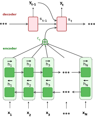
Figure 1: Computation of the decoder’s hidden state $\bm{s}_{t}$ using the attention mechanism.

We use a single-layer feed-forward neural network to initialise the decoder’s hidden state $\bm{s}_{0}$ at time step $t=0$ and feed it the concatenation of the last hidden states of the encoder’s forward RNN ($\overrightarrow{\Phi}_{\text{enc}}$) and backward RNN ($\overleftarrow{\Phi}_{\text{enc}}$), as in (5):

$$\bm{s}_{0}=\tanh\big{(}\bm{W}_{di}[\overleftarrow{\bm{h}}_{1};\overrightarrow{\bm{h}_{N}}]+\bm{b}_{di}\big{)},$$ (5)

where $\bm{W}_{di}$ and $\bm{b}_{di}$ are model parameters. Since RNNs normally better store information about recent inputs in comparison to more distant ones Hochreiter and Schmidhuber (1997); Bahdanau et al. (2015), we expect to initialise the decoder’s hidden state with a strong source sentence representation, i.e. a representation with a strong focus on both the first and the last tokens in the source sentence.

2.2 Multi-modal NMT (MNMT)

Our models can be seen as expansions of the attention-based NMT framework described in section 2 with the addition of a visual component to incorporate image features.

Simonyan and Zisserman Simonyan and Zisserman (2014) trained and evaluated an extensive set of deep convolutional neural network (CNN) models for classifying images into one out of the $1000$ classes in ImageNet Russakovsky et al. (2015). We use their 19-layer VGG network (VGG$19$) to extract image feature vectors for all images in our dataset. We feed an image to the pre-trained VGG$19$ network and use the $4096$D activations of the penultimate fully-connected layer FC$7$ as our image feature vector, henceforth referred to as $\bm{q}$.

We propose three different methods to incorporate images into the attentive NMT framework: using an image as words in the source sentence (Section 2.2.1), using an image to initialise the source language encoder (section 2.2.2) and the target language decoder (section 2.2.3).

We also evaluated a fourth mechanism to incorporate images into NMT, namely to use an image as one of the different contexts available to the decoder at each time step of the decoding process. We add the image features directly as an additional context, in addition to $\bm{W}_{y}[\tilde{y}_{t-1}]$, $\bm{s}_{t-1}$ and $\bm{c}_{t}$, to compute the hidden state $\bm{s}_{t}$ of the decoder at a given time step $t$. We corroborate previous findings by Vinyals et al. (2015) in that adding the image features as such causes the model to overfit, ultimately preventing learning.

2.2.1 Images as source words: IMG${}_{\text{W}}$

One way we propose to incorporate images into the encoder is to project an image feature vector into the space of the words of the source sentence. We use the projected image as the first and/or last word of the source sentence and let the attention model learn when to attend to the image representation. Specifically, given the global image feature vector $\bm{q}\in\mathbb{R}^{4096}$, we compute (6):

$$\bm{d}=\bm{W}_{I}^{2}\cdot(\bm{W}_{I}^{1}\cdot\bm{q}+\bm{b}_{I}^{1})+\bm{b}_{I}^{2},$$ (6)

where $\bm{W}_{I}^{1}\in\mathbb{R}^{4096\times 4096}$ and $\bm{W}_{I}^{2}\in\mathbb{R}^{4096\times d_{x}}$ are image transformation matrices, $\bm{b}_{I}^{1}\in\mathbb{R}^{4096}$ and $\bm{b}_{I}^{2}\in\mathbb{R}^{d_{x}}$ are bias vectors, and $d_{x}$ is the source words vector space dimensionality, all trained with the model. We then directly use $\bm{d}$ as words in the source words vector space: as the first word only (model IMG${}_{1\text{W}}$), and as the first and last words of the source sentence (model IMG${}_{2\text{W}}$).

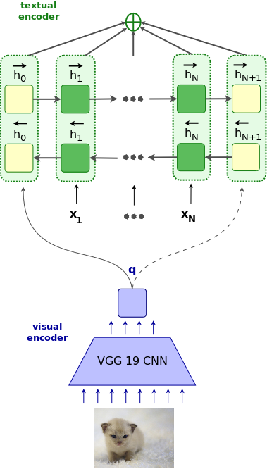
Figure 2: An encoder bidirectional RNN that uses image features as words in the source sequence.

An illustration of this idea is given in Figure 2, where a source sentence that originally contained $N$ tokens, after including the image as source words will contain $N+1$ tokens (model IMG${}_{1\text{W}}$) or $N+2$ tokens (model IMG${}_{2\text{W}}$). In model IMG${}_{1\text{W}}$, the image is projected as the first source word only (solid line in Figure 2); in model IMG${}_{2\text{W}}$, it is projected into the source words space as both first and last words (both solid and dashed lines in Figure 2).

Given a source sequence $X=(x_{1},x_{2},\cdots,x_{N})$, we concatenate the transformed image vector $\bm{d}$ to $\bm{W}_{x}[X]$ and apply the forward and backward encoder RNN passes, generating hidden vectors as in Figure 2. When computing the context vector $\bm{c}_{t}$ (Equations (2) and (3)), we effectively make use of the transformed image vector, i.e. the $\bm{\alpha}_{t,i}$ attention weight parameters will use this information to attend or not to the image features.

By including images into the encoder in models IMG${}_{1\text{W}}$ and IMG${}_{2\text{W}}$, our intuition is that (i) by including the image as the first word, we propagate image features into the source sentence vector representations when applying the forward RNN $\overrightarrow{\Phi}_{\text{enc}}$ (vectors $\overrightarrow{\bm{h}_{i}}$), and (ii) by including the image as the last word, we propagate image features into the source sentence vector representations when applying the backward RNN $\overleftarrow{\Phi}_{\text{enc}}$ (vectors $\overleftarrow{\bm{h}_{i}}$).

2.2.2 Images for encoder initialisation: IMG${}_{\text{E}}$

In the original attention-based NMT model described in section 2, the hidden state of the encoder is initialised with the zero vector $\vv{0}$. Instead, we propose to use two new single-layer feed-forward neural networks to compute the initial states of the forward RNN $\overrightarrow{\Phi}_{\text{enc}}$ and the backward RNN $\overleftarrow{\Phi}_{\text{enc}}$, respectively, as illustrated in Figure 3.

Similarly to section 2.2.1, given a global image feature vector $\bm{q}\in\mathbb{R}^{4096}$, we compute a vector $\bm{d}$ using Equation (6), only this time the parameters $\bm{W}_{I}^{2}$ and $\bm{b}_{I}^{2}$ project the image features into the same dimensionality as the textual encoder hidden states.

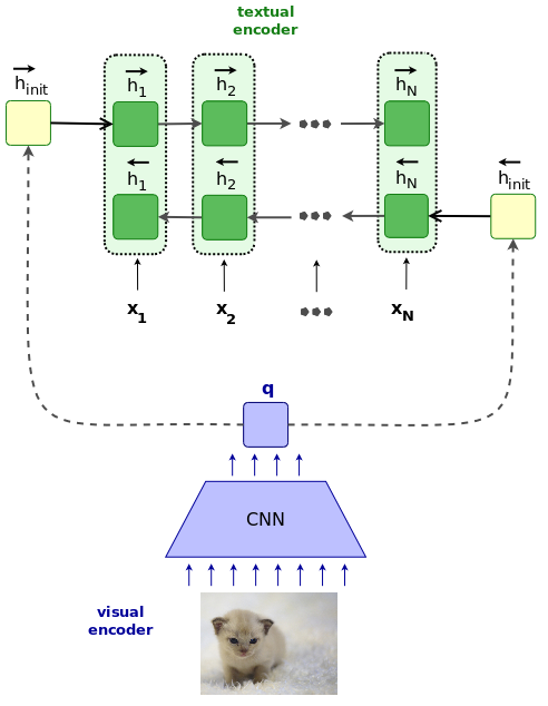
Figure 3: Using an image to initialise the encoder hidden states.

The feed-forward networks used to initialise the encoder hidden state are computed as in (2.2.2):

$$\overleftarrow{\bm{h}}_{\text{init}}=\tanh\big{(}\bm{W}_{f}\bm{d}+\bm{b}_{f}\big{)},$$

$$\overrightarrow{\bm{h}}_{\text{init}}=\tanh\big{(}\bm{W}_{b}\bm{d}+\bm{b}_{b}\big{)},$$ (7)

where $\bm{W}_{f}$ and $\bm{W}_{b}$ are multi-modal projection matrices that project the image features $\bm{d}$ into the encoder forward and backward hidden states dimensionality, respectively, and $\bm{b}_{f}$ and $\bm{b}_{b}$ are bias vectors.

2.2.3 Images for decoder initialisation: IMG${}_{\text{D}}$

To incorporate an image into the decoder, we introduce a new single-layer feed-forward neural network to be used instead of the one described in Equation 5. Originally, the decoder’s initial hidden state was computed using the concatenation of the last hidden states of the encoder forward RNN ($\overrightarrow{\Phi}_{\text{enc}}$) and backward RNN ($\overleftarrow{\Phi}_{\text{enc}}$), respectively $\overrightarrow{\bm{h}_{N}}$ and $\overleftarrow{\bm{h}}_{1}$.

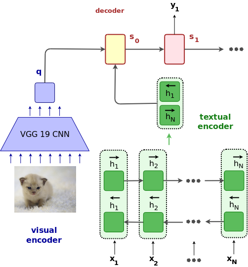
Figure 4: Image as additional data to initialise the decoder hidden state $s_{0}$.

Our proposal is that we include the image features as additional input to initialise the decoder hidden state at time step $t=0$, as in (8):

$$\bm{s}_{0}=\tanh\big{(}\bm{W}_{di}[\overleftarrow{\bm{h}}_{1};\overrightarrow{\bm{h}_{N}}]+\bm{W}_{m}\bm{d}+\bm{b}_{di}\big{)},$$ (8)

where $\bm{W}_{m}$ is a multi-modal projection matrix that projects the image features $\bm{d}$ into the decoder hidden state dimensionality and $\bm{W}_{di}$ and $\bm{b}_{di}$ are the same as in Equation (5).

Once again we compute $\bm{d}$ by applying Equation (6) onto a global image feature vector $\bm{q}\in\mathbb{R}^{4096}$, only this time the parameters $\bm{W}_{I}^{2}$ and $\bm{b}_{I}^{2}$ project the image features into the same dimensionality as the decoder hidden states. We illustrate this idea in Figure 4.

3 Data set

Our multi-modal NMT models need bilingual sentences accompanied by one or more images as training data. The original Flickr30k data set contains $30$k images and $5$ English sentence descriptions for each image Young et al. (2014). We use the translated and the comparable Multi30k datasets Elliott et al. (2016), henceforth referred to as M30k${}_{\text{T}}$ and M30k${}_{\text{C}}$, respectively, which are multilingual expansions of the original Flickr30k.

For each of the 30k images in the Flickr30k, the M30k${}_{\text{T}}$ has one of its English descriptions manually translated into German by a professional translator. Training, validation and test sets contain 29k, 1014 and 1k images, respectively, each accompanied by one sentence pair (the original English sentence and its German translation). For each of the 30k images in the Flickr30k, the M30k${}_{\text{C}}$ has five descriptions in German collected independently of the English descriptions. Training, validation and test sets contain 29k, 1014 and 1k images, respectively, each accompanied by five sentences in English and five sentences in German.

We use the scripts in the Moses SMT Toolkit Koehn et al. (2007) to normalise, truecase and tokenize English and German descriptions and we also convert space-separated tokens into subwords Sennrich et al. (2016b). All models use a common vocabulary of 83,093 English and 91,141 German subword tokens. If sentences in English or German are longer than 80 tokens, they are discarded.

We use the entire M30k${}_{\text{T}}$ training set for training, its validation set for model selection with BLEU, and its test set to evaluate our models. In order to study the impact that additional training data brings to the models, we use the baseline model described in section 2 trained on the textual part of the M30k${}_{\text{T}}$ data set (German$\rightarrow$English) without the images to build a back-translation model Sennrich et al. (2016a). We back-translate the $145$k German descriptions in the M30k${}_{\text{C}}$ into English and include the triples (synthetic English description, German description, image) as additional training data.

We train models to translate from English into German and report evaluation of cased, tokenized sentences with punctuation.

4 Experimental setup

Our encoder is a bidirectional RNN with GRU (one 1024D single-layer forward RNN and one 1024D single-layer backward RNN). Source and target word embeddings are 620D each and both are trained jointly with our model. All non-recurrent matrices are initialised by sampling from a Gaussian distribution $(\mu=0,\sigma=0.01)$, recurrent matrices are orthogonal and bias vectors are all initialised to zero. Our decoder RNN also uses GRU and is a neural LM Bengio et al. (2003) conditioned on its previous emissions and the source sentence by means of the source attention mechanism.

Image features are obtained by feeding images to the pre-trained VGG$19$ network of Simonyan and Zisserman Simonyan and Zisserman (2014) and using the activations of the penultimate fully-connected layer FC$7$. We apply dropout with a probability of $0.2$ in both source and target word embeddings and with a probability of $0.5$ in the image features (in all MNMT models), in the encoder and decoder RNNs inputs and recurrent connections, and before the readout operation in the decoder RNN. We follow Gal and Ghahramani (2016) and apply dropout to the encoder bidirectional RNN and decoder RNN using the same mask in all time steps.

Our models are trained using stochastic gradient descent with Adadelta Zeiler (2012) and minibatches of size 40, where each training instance consists of one English sentence, one German sentence and one image. We apply early stopping for model selection based on BLEU scores, so that if a model does not improve on BLEU in the validation set for more than 20 epochs, training is halted.

We evaluate our models’ translation quality quantitatively in terms of BLEU$4$ Papineni et al. (2002), METEOR Denkowski and Lavie (2014), TER Snover et al. (2006), and chrF3 scores Popović (2015) and we report statistical significance for the three first metrics using approximate randomisation computed with MultEval Clark et al. (2011).

As our main baseline we train an attention-based NMT model (section 2) in which only the textual part of M30k${}_{\text{T}}$ is used for training. We also train a PBSMT model built with Moses on the same data. The LM is a 5–gram LM with modified Kneser-Ney smoothing Kneser and Ney (1995) trained on the German side of the M30k${}_{\text{T}}$ dataset. We use minimum error rate training Och (2003) for tuning the model parameters for BLEU scores. Our third baseline is the best comparable multi-modal model by Huang et al. (2016) and also their best model with additional object detections: respectively models m1 (image at head) and m3 in the authors’ paper.

4.1 Results

	BLEU$4$$\uparrow$	METEOR$\uparrow$	TER$\downarrow$	chrF3$\uparrow$
PBSMT	32.9	54.1	45.1	67.4
NMT	33.7	52.3	46.7	64.5
Huang	35.1	52.2	—	—
+ RCNN	36.5	54.1	—	—
IMG${}_{1\text{W}}$	37.1†‡ ($\uparrow$ 3.4)	54.5†‡ ($\uparrow$ 0.4)	42.7†‡ ($\downarrow$ 2.4)	66.9 ($\downarrow$ 0.5)
IMG${}_{2\text{W}}$	36.9†‡ ($\uparrow$ 3.2)	54.3†‡ ($\uparrow$ 0.2)	41.9†‡ ($\downarrow$ 3.2)	66.8 ($\downarrow$ 0.6)
IMG${}_{\text{E}}$	37.1†‡ ($\uparrow$ 3.4)	55.0†‡ ($\uparrow$ 0.9)	43.1†‡ ($\downarrow$ 2.0)	67.6 ($\uparrow$ 0.2)
IMG${}_{\text{D}}$	37.3†‡ ($\uparrow$ 3.6)	55.1†‡ ($\uparrow$ 1.0)	42.8†‡ ($\downarrow$ 2.3)	67.7 ($\uparrow$ 0.3)
IMG${}_{2\text{W+D}}$	35.7†‡ ($\uparrow$ 2.0)	53.6†‡ ($\downarrow$ 0.5)	43.3†‡ ($\downarrow$ 1.8)	66.2 ($\downarrow$ 1.2)
IMG${}_{\text{E+D}}$	37.0†‡ ($\uparrow$ 3.3)	54.7†‡ ($\uparrow$ 0.6)	42.6†‡ ($\downarrow$ 2.5)	67.2 ($\downarrow$ 0.2)

Table 1: BLEU$4$, METEOR, chrF3 (higher is better) and TER scores (lower is better) on the M30k${}_{\text{T}}$ test set for the two text-only baselines PBSMT and NMT, the two multi-modal NMT models by Huang et al. (2016) and our MNMT models that: (i) use images as words in the source sentence (IMG${}_{1\text{W}}$, IMG${}_{2\text{W}}$), (ii) use images to initialise the encoder (IMG${}_{\text{E}}$), and (iii) use images as additional data to initialise the decoder (IMG${}_{\text{D}}$). Best text-only baselines are underscored and best overall results appear in bold. We highlight in parentheses the improvements brought by our models compared to the best corresponding text-only baseline score. Results differ significantly from PBSMT baseline ($\dagger$) or NMT baseline ($\ddagger$) with $p=0.05$.

The Multi30K dataset contains images and bilingual descriptions. Overall, it is a small dataset with a small vocabulary whose sentences have simple syntactic structures and not much ambiguity Elliott et al. (2016). This is reflected in the fact that even the simplest baselines perform fairly well on it, i.e. the smallest BLEU score of 32.9 is that of the PBSMT model, which is still good for translating into German.

From Table 1 we see that our multi-modal models perform well, with models IMG${}_{\text{E}}$ and IMG${}_{\text{D}}$ improving on both baselines according to all metrics analysed. We also note that all models but IMG${}_{\text{2W+D}}$ perform consistently better than the strong multi-modal NMT baseline of Huang et al. (2016), even when this model has access to more data (+RCNN features). Combining image features in the encoder and the decoder at the same time (last two entries in Table 1) does not seem to improve results compared to using the image features in only the encoder or the decoder. To the best of our knowledge, it is the first time a purely neural model significantly improves over a PBSMT model in all metrics on this data set.

Arguably, the main downside of applying multi-modal NMT in a real-world scenario is the small amount of publicly available training data ($\sim$$30$k), which restricts its applicability. For that reason, we back-translated the German sentences in the M30k${}_{\text{C}}$ and created additional $145$k synthetic triples (synthetic English sentence, original German sentence and image).

In Table 2, we present results for some of the models evaluated in Table 1 but when also trained on the additional data. In order to add more data to the PBSMT baseline, we simply added the German sentences in the M30k${}_{\text{C}}$ as additional data to train the LM. Both our models IMG${}_{\text{E}}$ and IMG${}_{\text{D}}$ that use global image features to initialise the encoder and the decoder, respectively, improve significantly according to BLEU, METEOR and TER with the additional back-translated data, and also achieved better chrF3 scores. Model IMG${}_{\text{2W}}$, that uses images as words in the source sentence, does not significantly differ in BLEU, METEOR or TER ($p=0.05$), but achieves a lower chrF3 score than the comparable PBSMT model. Although model IMG${}_{\text{2W}}$ trained on only the original data has the best TER score ($=41.9$), both models IMG${}_{\text{E}}$ and IMG${}_{\text{D}}$ perform comparably with the additional back-translated data ($=41.4$ and $41.6$, respectively), though the difference between the latter and the former is still not statistically significant ($p=0.05$).

We see in Tables 1 and 2 that our models that use images directly to initialise either the encoder or the decoder are the only ones to consistently outperform the PBSMT baseline according to the chrF3 metric, a character-based metric that includes both precision and recall, and has a recall bias. That is also a noteworthy finding, since chrF3 is the only character-level metric we use, and it has shown a high correlation with human judgements Stanojević et al. (2015).

In Table 3 we see translations for two entries in the test M30k set. In the first entry, although the reference translation is incorrect—there is just one dog in the image—, the multi-modal models translated it correctly. In the second entry, the last three multi-modal models extrapolate the reference+image and describe “ceremony” as a “wedding ceremony” (IMG${}_{\text{2W}}$) and as an “Olympics ceremony” (IMG${}_{\text{E}}$ and IMG${}_{\text{D}}$). This could be due to the fact that the training set is small, depicts a small variation of different scenes and contains different forms of biasses van Miltenburg (2015).

We note that the idea of using images as words in the source sentence, also entertained by Huang et al. (2016), does not perform as well as directly using the images in the encoder or decoder initialisation. The fact that multi-modal NMT models can benefit from back-translated data is also an interesting finding.

	BLEU$4$$\uparrow$	METEOR$\uparrow$	TER$\downarrow$	chrF3$\uparrow$
original training data
IMG${}_{2\text{W}}$	36.9	54.3	41.9	66.8
IMG${}_{\text{E}}$	37.1	55.0	43.1	67.6
IMG${}_{\text{D}}$	37.3	55.1	42.8	67.7
+ back-translated training data
PBSMT	34.0	55.0	44.7	68.0
NMT	35.5	53.4	43.3	65.3
IMG${}_{2\text{W}}$	36.7†‡ ($\uparrow$ 1.2)	54.6†‡ ($\downarrow$ 0.4)	42.0†‡ ($\downarrow$ 1.3)	66.8 ($\downarrow$ 1.2)
IMG${}_{\text{E}}$	38.5†‡ ($\uparrow$ 3.0)	55.7†‡ ($\uparrow$ 0.9)	41.4†‡ ($\downarrow$ 1.9)	68.3 ($\uparrow$ 0.3)
IMG${}_{\text{D}}$	38.5†‡ ($\uparrow$ 3.0)	55.9†‡ ($\uparrow$ 1.1)	41.6†‡ ($\downarrow$ 1.7)	68.4 ($\uparrow$ 0.4)
Improvements (original vs. + back-translated)
IMG${}_{\text{2W}}$	$\downarrow$ 0.2	$\uparrow$ 0.1	$\uparrow$ 0.1	$\uparrow$ 0.0
IMG${}_{\text{E}}$	$\uparrow$ 1.4	$\uparrow$ 0.7	$\downarrow$ 1.8	$\uparrow$ 0.7
IMG${}_{\text{D}}$	$\uparrow$ 1.2	$\uparrow$ 0.8	$\downarrow$ 1.2	$\uparrow$ 0.7

Table 2: BLEU$4$, METEOR, TER and chrF3 scores on the M30k${}_{\text{T}}$ test set for models trained on original and additional back-translated data. Best text-only baselines are underscored and best overall results in bold. We highlight in parentheses the improvements brought by our models compared to the best baseline score. Results differ significantly from PBSMT baseline ($\dagger$) or NMT baseline ($\ddagger$) with $p=0.05$. We also show the improvements each model yields in each metric when only trained on the original M30k${}_{\text{T}}$ training set vs. also including additional back-translated data.

ref.	ein brauner und ein schwarzer Hund laufen auf
	einem Pfad im Wald.
SMT	ein braun und schwarzer Hund läuft auf einem
	Pfad im Wald.
NMT	ein brauner Hund steht an einem Sand Strand.
IMG${}_{\text{1W}}$	ein braun-schwarzer Hund läuft auf einem Pfad im Wald.
IMG${}_{\text{2W}}$	ein braun-schwarzer Hund läuft im Wald auf einem Pfad.
IMG${}_{\text{E}}$	ein braun-schwarzer Hund läuft im Wald auf einem Pfad.
IMG${}_{\text{D}}$	ein braun-schwarzer Hund läuft im Wald auf einem Pfad.
ref.	eine Frau mit langen Haaren bei einer Abschluss Feier.
SMT	eine Frau mit langen Haaren steht an einem Abschluss
NMT	eine Frau mit langen Haaren ist an einer StaZeremonie.
IMG${}_{\text{1W}}$	eine Frau mit langen Haaren ist an einer warmen
	Zeremonie teil.
IMG${}_{\text{2W}}$	eine Frau mit langen Haaren steht bei einer Hochzeit Feier.
IMG${}_{\text{E}}$	eine lang haarige Frau bei einer olympischen Zeremonie.
IMG${}_{\text{D}}$	eine lang haarige Frau bei einer olympischen Zeremonie.

Table 3: Some translations for the M30k test set.

5 Conclusions

We have introduced different ideas to incorporate images into state-of-the-art attention-based NMT, by using images as words in the source sentence, to initialise the encoder’s hidden state and as additional data in the initialisation of the decoder’s hidden state. We corroborate previous findings in that using image features directly at each time step of the decoder causes the model to overfit and prevents learning. The intuition behind our effort is to use global image feature vectors to visually ground translations and consequently increase translation quality. Extensive experiments show that adding global image features into attention-based NMT is useful and improves over NMT and PBSMT as well as a strong multi-modal NMT baseline, according to all metrics evaluated.

In future work we will conduct a more systematic study on the impact that synthetic back-translated data can have on multi-modal NMT, and also investigate how to incorporate local, spatial-preserving image features.

References

- Bahdanau et al. (2015) Dzmitry Bahdanau, Kyunghyun Cho, and Yoshua Bengio. 2015. Neural Machine Translation by Jointly Learning to Align and Translate. In International Conference on Learning Representations, ICLR 2015. San Diego, California.
- Bengio et al. (2015) Samy Bengio, Oriol Vinyals, Navdeep Jaitly, and Noam M. Shazeer. 2015. Scheduled Sampling for Sequence Prediction with Recurrent Neural Networks. In Advances in Neural Information Processing Systems, NIPS. http://arxiv.org/abs/1506.03099.
- Bengio et al. (2003) Yoshua Bengio, Réjean Ducharme, Pascal Vincent, and Christian Janvin. 2003. A Neural Probabilistic Language Model. J. Mach. Learn. Res. 3:1137–1155. http://dl.acm.org/citation.cfm?id=944919.944966.
- Caglayan et al. (2016) Ozan Caglayan, Walid Aransa, Yaxing Wang, Marc Masana, Mercedes García-Martínez, Fethi Bougares, Loïc Barrault, and Joost van de Weijer. 2016. Does Multimodality Help Human and Machine for Translation and Image Captioning? In Proceedings of the First Conference on Machine Translation. Berlin, Germany, pages 627–633. http://www.aclweb.org/anthology/W/W16/W16-2358.
- Calixto et al. (2012) Iacer Calixto, Teofilo de Campos, and Lucia Specia. 2012. Images as context in Statistical Machine Translation. In Proceedings of the Workshop on Vision and Language, VL 2012. Sheffield, England.
- Calixto et al. (2016) Iacer Calixto, Desmond Elliott, and Stella Frank. 2016. DCU-UvA Multimodal MT System Report. In Proceedings of the First Conference on Machine Translation. Berlin, Germany, pages 634–638. http://www.aclweb.org/anthology/W/W16/W16-2359.
- Cho et al. (2014a) Kyunghyun Cho, Bart van Merriënboer, Dzmitry Bahdanau, and Yoshua Bengio. 2014a. On the properties of neural machine translation: Encoder–decoder approaches. Syntax, Semantics and Structure in Statistical Translation page 103.
- Cho et al. (2014b) Kyunghyun Cho, Bart van Merrienboer, Caglar Gulcehre, Dzmitry Bahdanau, Fethi Bougares, Holger Schwenk, and Yoshua Bengio. 2014b. Learning Phrase Representations using RNN Encoder–Decoder for Statistical Machine Translation. In Proceedings of the 2014 Conference on Empirical Methods in Natural Language Processing (EMNLP). Doha, Qatar, pages 1724–1734. http://www.aclweb.org/anthology/D14-1179.
- Clark et al. (2011) Jonathan H. Clark, Chris Dyer, Alon Lavie, and Noah A. Smith. 2011. Better Hypothesis Testing for Statistical Machine Translation: Controlling for Optimizer Instability. In Proceedings of the 49th Annual Meeting of the Association for Computational Linguistics: Human Language Technologies: Short Papers - Volume 2. Portland, Oregon, HLT ’11, pages 176–181. http://dl.acm.org/citation.cfm?id=2002736.2002774.
- Denkowski and Lavie (2014) Michael Denkowski and Alon Lavie. 2014. Meteor Universal: Language Specific Translation Evaluation for Any Target Language. In Proceedings of the EACL 2014 Workshop on Statistical Machine Translation.
- Donahue et al. (2015) Jeff Donahue, Lisa Anne Hendricks, Sergio Guadarrama, Marcus Rohrbach, Subhashini Venugopalan, Trevor Darrell, and Kate Saenko. 2015. Long-term Recurrent Convolutional Networks for Visual Recognition and Description. In Computer Vision and Pattern Recognition (CVPR), 2015 IEEE Conference on. Boston, US, pages 2625–2634.
- Dong et al. (2015) Daxiang Dong, Hua Wu, Wei He, Dianhai Yu, and Haifeng Wang. 2015. Multi-Task Learning for Multiple Language Translation. In Proceedings of the 53rd Annual Meeting of the Association for Computational Linguistics and the 7th International Joint Conference on Natural Language Processing (Volume 1: Long Papers). Beijing, China, pages 1723–1732. http://www.aclweb.org/anthology/P15-1166.
- Elliott et al. (2015) Desmond Elliott, Stella Frank, and Eva Hasler. 2015. Multi-language image description with neural sequence models. CoRR abs/1510.04709. http://arxiv.org/abs/1510.04709.
- Elliott et al. (2016) Desmond Elliott, Stella Frank, Khalil Sima’an, and Lucia Specia. 2016. Multi30K: Multilingual English-German Image Descriptions. In Proceedings of the 5th Workshop on Vision and Language, VL@ACL 2016. Berlin, Germany. http://aclweb.org/anthology/W/W16/W16-3210.pdf.
- Firat et al. (2016) Orhan Firat, Kyunghyun Cho, and Yoshua Bengio. 2016. Multi-Way, Multilingual Neural Machine Translation with a Shared Attention Mechanism. In Proceedings of the 2016 Conference of the North American Chapter of the Association for Computational Linguistics: Human Language Technologies. San Diego, California, pages 866–875. http://www.aclweb.org/anthology/N16-1101.
- Gal and Ghahramani (2016) Yarin Gal and Zoubin Ghahramani. 2016. A Theoretically Grounded Application of Dropout in Recurrent Neural Networks. In Advances in Neural Information Processing Systems, NIPS, Barcelona, Spain, pages 1019–1027. http://papers.nips.cc/paper/6241-a-theoretically-grounded-application-of-dropout-in-recurrent-neural-networks.pdf.
- Girshick et al. (2014) Ross Girshick, Jeff Donahue, Trevor Darrell, and Jitendra Malik. 2014. Rich Feature Hierarchies for Accurate Object Detection and Semantic Segmentation. In Proceedings of the 2014 IEEE Conference on Computer Vision and Pattern Recognition. Washington, DC, USA, CVPR ’14, pages 580–587. https://doi.org/10.1109/CVPR.2014.81.
- Graves (2013) Alex Graves. 2013. Generating Sequences With Recurrent Neural Networks. CoRR abs/1308.0850. http://arxiv.org/abs/1308.0850.
- Hitschler et al. (2016) Julian Hitschler, Shigehiko Schamoni, and Stefan Riezler. 2016. Multimodal Pivots for Image Caption Translation. In Proceedings of the 54th Annual Meeting of the Association for Computational Linguistics (Volume 1: Long Papers). Berlin, Germany, pages 2399–2409. http://www.aclweb.org/anthology/P16-1227.
- Hochreiter and Schmidhuber (1997) Sepp Hochreiter and Jürgen Schmidhuber. 1997. Long Short-Term Memory. Neural Comput. 9(8):1735–1780. https://doi.org/10.1162/neco.1997.9.8.1735.
- Hodosh et al. (2013) Micah Hodosh, Peter Young, and Julia Hockenmaier. 2013. Framing Image Description As a Ranking Task: Data, Models and Evaluation Metrics. J. Artif. Int. Res. 47(1):853–899. http://dl.acm.org/citation.cfm?id=2566972.2566993.
- Huang et al. (2016) Po-Yao Huang, Frederick Liu, Sz-Rung Shiang, Jean Oh, and Chris Dyer. 2016. Attention-based Multimodal Neural Machine Translation. In Proceedings of the First Conference on Machine Translation. Berlin, Germany, pages 639–645. http://www.aclweb.org/anthology/W/W16/W16-2360.
- Kalchbrenner and Blunsom (2013) Nal Kalchbrenner and Phil Blunsom. 2013. Recurrent Continuous Translation Models. In Proceedings of the 2013 Conference on Empirical Methods in Natural Language Processing, EMNLP 2013. Seattle, pages 1700–1709.
- Karpathy and Fei-Fei (2015) Andrej Karpathy and Li Fei-Fei. 2015. Deep visual-semantic alignments for generating image descriptions. In Proceedings of the IEEE Conference on Computer Vision and Pattern Recognition, CVPR 2015. Boston, Massachusetts, pages 3128–3137.
- Kiros et al. (2014) Ryan Kiros, Ruslan Salakhutdinov, and Richard S. Zemel. 2014. Unifying visual-semantic embeddings with multimodal neural language models. CoRR abs/1411.2539. http://arxiv.org/abs/1411.2539.
- Kneser and Ney (1995) Reinhard Kneser and Hermann Ney. 1995. Improved backing-off for m-gram language modeling. In In Proceedings of the IEEE International Conference on Acoustics, Speech and Signal Processing. Detroit, Michigan, volume I, pages 181–184.
- Koehn et al. (2007) Philipp Koehn, Hieu Hoang, Alexandra Birch, Chris Callison-Burch, Marcello Federico, Nicola Bertoldi, Brooke Cowan, Wade Shen, Christine Moran, Richard Zens, Chris Dyer, Ondřej Bojar, Alexandra Constantin, and Evan Herbst. 2007. Moses: Open Source Toolkit for Statistical Machine Translation. In Proceedings of the 45th Annual Meeting of the ACL on Interactive Poster and Demonstration Sessions. Association for Computational Linguistics, Prague, Czech Republic, ACL ’07, pages 177–180. http://dl.acm.org/citation.cfm?id=1557769.1557821.
- Libovický et al. (2016) Jindřich Libovický, Jindřich Helcl, Marek Tlustý, Ondřej Bojar, and Pavel Pecina. 2016. CUNI System for WMT16 Automatic Post-Editing and Multimodal Translation Tasks. In Proceedings of the First Conference on Machine Translation. Berlin, Germany, pages 646–654. http://www.aclweb.org/anthology/W/W16/W16-2361.
- Luong et al. (2016) Minh-Thang Luong, Quoc V. Le, Ilya Sutskever, Oriol Vinyals, and Lukasz Kaiser. 2016. Multi-Task Sequence to Sequence Learning. In Proceedings of the International Conference on Learning Representations (ICLR), 2016. San Juan, Puerto Rico.
- Luong et al. (2015) Thang Luong, Hieu Pham, and Christopher D. Manning. 2015. Effective Approaches to Attention-based Neural Machine Translation. In Proceedings of the 2015 Conference on Empirical Methods in Natural Language Processing (EMNLP). Lisbon, Portugal, pages 1412–1421.
- Mao et al. (2014) Junhua Mao, Wei Xu, Yi Yang, Jiang Wang, and Alan L. Yuille. 2014. Explain Images with Multimodal Recurrent Neural Networks. http://arxiv.org/abs/1410.1090.
- Och (2003) Franz Josef Och. 2003. Minimum Error Rate Training in Statistical Machine Translation. In Proceedings of the 41st Annual Meeting on Association for Computational Linguistics - Volume 1. Sapporo, Japan, ACL ’03, pages 160–167. https://doi.org/10.3115/1075096.1075117.
- Papineni et al. (2002) Kishore Papineni, Salim Roukos, Todd Ward, and Wei-Jing Zhu. 2002. BLEU: A Method for Automatic Evaluation of Machine Translation. In Proceedings of the 40th Annual Meeting on Association for Computational Linguistics. Philadelphia, Pennsylvania, ACL ’02, pages 311–318. https://doi.org/10.3115/1073083.1073135.
- Popović (2015) Maja Popović. 2015. chrf: character n-gram f-score for automatic mt evaluation. In Proceedings of the Tenth Workshop on Statistical Machine Translation. Lisbon, Portugal, pages 392–395. http://aclweb.org/anthology/W15-3049.
- Russakovsky et al. (2015) Olga Russakovsky, Jia Deng, Hao Su, Jonathan Krause, Sanjeev Satheesh, Sean Ma, Zhiheng Huang, Andrej Karpathy, Aditya Khosla, Michael Bernstein, Alexander C. Berg, and Li Fei-Fei. 2015. ImageNet Large Scale Visual Recognition Challenge. International Journal of Computer Vision (IJCV) 115(3):211–252. https://doi.org/10.1007/s11263-015-0816-y.
- Sennrich et al. (2016a) Rico Sennrich, Barry Haddow, and Alexandra Birch. 2016a. Improving Neural Machine Translation Models with Monolingual Data. In Proceedings of the 54th Annual Meeting of the Association for Computational Linguistics (Volume 1: Long Papers). Berlin, Germany, pages 86–96. http://www.aclweb.org/anthology/P16-1009.
- Sennrich et al. (2016b) Rico Sennrich, Barry Haddow, and Alexandra Birch. 2016b. Neural Machine Translation of Rare Words with Subword Units. In Proceedings of the 54th Annual Meeting of the Association for Computational Linguistics (Volume 1: Long Papers). Berlin, Germany, pages 1715–1725. http://www.aclweb.org/anthology/P16-1162.
- Shah et al. (2016) Kashif Shah, Josiah Wang, and Lucia Specia. 2016. SHEF-Multimodal: Grounding Machine Translation on Images. In Proceedings of the First Conference on Machine Translation. Berlin, Germany, pages 660–665. http://www.aclweb.org/anthology/W/W16/W16-2363.