Ground-State Properties of ⁴He and ¹⁶O
Extrapolated from Lattice QCD with Pionless EFT

Abstract

We extend the prediction range of Pionless Effective Field Theory with an analysis of the ground state of ¹⁶O in leading order. To renormalize the theory, we use as input both experimental data and lattice QCD predictions of nuclear observables, which probe the sensitivity of nuclei to increased quark masses. The nuclear many-body Schrödinger equation is solved with the Auxiliary Field Diffusion Monte Carlo method. For the first time in a nuclear quantum Monte Carlo calculation, a linear optimization procedure, which allows us to devise an accurate trial wave function with a large number of variational parameters, is adopted. The method yields a binding energy of ⁴He which is in good agreement with experiment at physical pion mass and with lattice calculations at larger pion masses. At leading order we do not find any evidence of a ¹⁶O state which is stable against breakup into four ⁴He, although higher-order terms could bind ¹⁶O.

1 Introduction

Establishing a clear path leading from the fundamental theory of strong interactions, namely Quantum Chromodynamics (QCD), to nuclear observables, such as nuclear masses and electroweak transitions, is one of the main goals of modern nuclear theory. At present, the most reliable numerical technique to perform QCD calculations is Lattice QCD (LQCD). It combines recent advances in high-performance computing, innovative algorithms, and conceptual breakthroughs in nuclear theory to produce predictions of nucleon-nucleon scattering, and the binding energies and magnetic moments of light nuclei. However, there are technical problems, which have so far limited the applicability of LQCD to $A\leq 4$ baryon systems and to artificially large quark masses. Then, LQCD calculations require significantly smaller computational resources to yield meaningful signal-to-noise ratios. In this paper, we consider as examples LQCD data sets comprised of binding energies obtained at pion masses of $m_{\pi}\simeq 805$ MeV [1] and $m_{\pi}\simeq 510$ MeV [2].

The link between QCD and the entire nuclear landscape is a potential whose systematic derivation was developed in the framework of effective field theory (EFT) in the last two decades [3, 4, 5]. This is achieved by exploiting a separation between “hard” ($M$) and “soft” ($Q$) momentum scales. The active degrees of freedom at soft scales are hadrons whose interactions are consistent with QCD. Effective potentials and currents are derived from the most general Lagrangian constrained by the QCD symmetries, and employed with standard few- and many-body techniques to make predictions for nuclear observables in a systematic expansion in $Q/M$. The interactions strengths carry information about the details of the QCD dynamics, and can be obtained by matching observables calculated in EFT and LQCD.

The aim of this work is the first extension of this program to the realm of medium-heavy nuclei. By using Pionless EFT (EFT($\not{\pi}$)) coupled to the Auxiliary Field Diffusion Monte Carlo (AFDMC) method [6] we analyze the connection between the ground state of ¹⁶O and its nucleon constituents. Beside physical data, the consideration of higher quark-mass input allows us to investigate the sensitivity of ¹⁶O stability to the pion mass. The usefulness of EFT($\not{\pi}$) [3, 4] for the analysis of LQCD calculations has been discussed previously [7, 8, 9].

Whether EFT($\not{\pi}$) can be extended to real and lattice nuclei in the medium-mass region is an open question. For physical pion mass, convergence has been demonstrated in leading orders for the low-energy properties of $A=2,3$ systems [10, 11, 12, 13]. Counterintuitively, the binding energy of the $A=4$ ground state was found in good agreement with experiment at leading order (LO) [14], and even the $A=6$ ground state comes out reasonably well at this order [15].

A similar binding energy per nucleon for ⁴He ($\simeq 7$ MeV) and ¹⁶O ($\simeq 8$ MeV) suggests that EFT($\not{\pi}$) might converge for heavier systems. However, the difference in total binding energy between the two systems is quite large. Moreover, many-body effects become stronger, and quantum correlations might substantially change the picture. We chose ¹⁶O for mainly two reasons: First, because it is a doubly magic nucleus, thereby reducing the technical difficulties related to the construction of wave functions with the correct quantum numbers and symmetries. Second, its central density is sufficiently high to probe saturation properties and thereby serve as a model for even heavier nuclei.

In practice, this first calculation of an $A>6$ system in EFT($\not{\pi}$) at LO is carried out as follows. In order to show renormalizability, we use potentials characterized by cutoffs up to $\simeq 1.5$ GeV. This introduces non-trivial difficulties in solving the Schrödinger equation due to the rapidly changing behavior of the wave functions. To this aim, we developed an efficient linear optimization scheme to devise high-quality variational wave functions. Those have been employed as a starting point for the imaginary-time projection of AFDMC which enhances the ground-state component of the trial wave function. Finally, to alleviate the sign problem, we have also performed unconstrained propagations and studied their convergence pattern. We show that, thanks to these developments, the errors from the AFDMC calculation are now much smaller than the uncertainty originating from the EFT($\not{\pi}$) truncation and the LQCD input. The door is open for higher-order calculations with future, more precise LQCD input.

The rest of the paper is organized as follows: in Sec. 2 we will briefly review the properties of EFT($\not{\pi}$) that are relevant for our discussion; in Sec. 3 the methodological aspect of the calculations will be discussed; in Sec. 4 we will present and discuss our results; and finally Sec. 5 is devoted to conclusions. An appendix describes the way we estimate errors.

2 Pionless Effective Field Theory

An EFT is a reformulation of an underlying theory in terms of degrees of freedom relevant to the problem at hand, which interact via operators that obey symmetries compatible with the original interactions. These operators are part of a controlled expansion in a suitable small parameter which encapsulates a separation of scales in the system.

The relativistic, underlying theory, which presumably allows for the description of nuclei from first principles, is QCD. Low-energy processes in nuclear physics involve small enough momenta to justify the use of a nonrelativistic approach. Consequently, nucleon number is conserved and nuclear dynamics can be described within nonrelativistic many-body theory, while the strong nuclear potential needs to include only parity and time-reversal conserving operators. All relativistic corrections are sub-leading.

In this paper we are interested in the ground states of nuclei. The characteristic momentum in a two-body bound state of binding energy $B_{2}$ is given by the location of the pole of the $S$ matrix in the complex momentum plane, $Q_{2}=\sqrt{m_{N}B_{2}}$, where $m_{N}$ is the nucleon mass. To our knowledge, there is no consensus for a definition of an analogous characteristic momentum for larger nuclei bound by $B_{A}$; as an estimate one can use a generalization where each nucleon contributes equally,

$$Q_{A}=\sqrt{2m_{N}\frac{B_{A}}{A}}\,.$$ (1)

For lattice ⁴He at $m_{\pi}=805$ MeV ($m_{\pi}=510$ MeV), where $B_{4}\simeq 110$ MeV [1] ($B_{4}\simeq 40$ MeV [2]) with $m_{N}\simeq 1600$ MeV ($m_{N}\simeq 1300$ MeV), this estimate gives $Q_{4}/m_{\pi}\simeq 0.4\;(0.3)$. Thus, the typical momentum is small in comparison not only with $m_{N}$, but also with $m_{\pi}$, allowing for a description where pion exchanges are treated as unresolved contact interactions. The case is less clear-cut in the real world, where $Q_{4}/m_{\pi}\simeq 0.8$, but the results at LO [14] suggest that Eq. (1) overestimates the typical momentum. In fact, a similar inference can be made from results of the analog of EFT($\not{\pi}$) for ⁴He atomic clusters [16]. At physical $m_{\pi}$, the binding energy per particle in ¹⁶O is similar to that in ⁴He, so EFT($\not{\pi}$) might converge for this nucleus as well.

With pions integrated out, $m_{\pi}$ gives an upper bound on the breakdown scale $M$ of the EFT. The momentum associated with nucleon excitations of mass $m_{R}$ is given by Eq. (1) with $B_{A}/A\to m_{R}-m_{N}$. For the lightest excitation, the Delta isobar, $m_{\Delta}-m_{N}$ decreases as $m_{\pi}$ increases. For $m_{\pi}=805$ MeV, $\sqrt{2m_{N}(m_{\Delta}-m_{N})}$ becomes comparable to $m_{\pi}$. Thus, throughout the considered range of pion masses nucleon resonances can also be treated as short-range effects, and nucleons are indeed the only relevant degrees of freedom.

At leading order in $1/M$, the EFT($\not{\pi}$) Lagrangian [17, 10, 18] consists of the nucleon kinetic term, two two-nucleon contact interactions, and one three-nucleon contact interaction. The singularity of these interactions leads to divergences that need to be dealt with by regularization and renormalization. Here, as in Refs. [7, 9], we use a Gaussian regulator that suppresses transferred momenta above an ultraviolet cutoff $\Lambda$. This choice ensures that the Lagrangian can be transformed into a Hamiltonian containing only local potentials, suitable to be used within AFDMC. The Hamiltonian in coordinate space reads [7, 9]

$$H_{LO} = -\sum_{i}\frac{{\vec{\nabla}_{i}^{2}}}{2m_{N}}+\sum_{i<j}{\left(C_{1}+C_{2}\,\vec{\sigma_{i}}\cdot\vec{\sigma_{j}}\right)e^{-r_{ij}^{2}\Lambda^{2}/4}}$$ (2)

$$+D_{0}\sum_{i<j<k}\sum_{\text{cyc}}{e^{-\left(r_{ik}^{2}+r_{ij}^{2}\right)\Lambda^{2}/4}}\,,$$

where the sums are over, respectively, nucleons, nucleon pairs, and nucleon triplets, and $\sum_{\text{cyc}}$ stands for the cyclic permutation of $i$, $j$, and $k$. Dependence on the arbitrary regulator choice is eliminated by allowing the interaction strengths, or low-energy constants (LECs), $C_{1}(\Lambda)$, $C_{2}(\Lambda)$ and $D_{0}(\Lambda)$ to depend on $\Lambda$.

To solve the two-nucleon system, in principle one iterates interactions only in the channels containing $S$-matrix poles within the convergence range of the theory [19]. Since two nucleons have a bound state in the ${}^{3}S_{1}$ channel and a shallow virtual state (which becomes a bound state as $m_{\pi}$ increases [1, 2]) in the ${}^{1}S_{0}$ channel, one needs to include two interactions at LO and treat them non-perturbatively. In Eq. (2) we chose the operator basis $1$ and $\vec{\sigma_{i}}\cdot\vec{\sigma_{j}}$, but it can by replaced by any other form equivalent under Fierz transformations in SU(2). All these possible choices are equally convenient for an AFDMC calculation.

When the three-body problem is solved with these interactions, renormalizability requires a contact three-nucleon force at LO [20]. As for the two-body interactions, there is some freedom in choosing the operator to include in the Hamiltonian formulation of the three-body force. For simplicity we use a central potential, which makes obvious the Wigner spin-isospin symmetry (SU(4)) of this force.

For renormalization at LO, we ensure that three uncorrelated observables are $\Lambda$-independent. Here we follow Ref. [9] and choose these observables as the deuteron and triton binding energies and, for physical (unphysical) pion mass(es) the ${}^{1}S_{0}$ scattering length (dineutron binding energy). The LECs’ dependence on the cutoff can be found in Ref. [9]. In particular, because $C_{1}(\Lambda)\gg C_{2}(\Lambda)$, the LO Hamiltonian has an approximate SU(4) symmetry.

Interactions with more derivatives represent higher orders. For example, at NLO the first two-body energy corrections appear in the form of two-derivative contact interactions [19]. For ground states electromagnetic interactions are also sub-leading, starting at NLO with the Coulomb interaction [13]. Since sub-leading interactions are suppressed by powers of $M$, they should be included as perturbations. Treating them non-perturbatively, like the LO terms, is problematic as the iteration of sub-leading terms usually destroys renormalizability. NLO interactions have been dealt with fully perturbatively for $A=2$ [10, 11] and $A=3$ [12, 13]. So far, no perturbative NLO calculation has been conducted in EFT($\not{\pi}$) for $A\geq 4$. We therefore limit ourselves to LO in this first foray into medium-mass nuclei.

One feature of the EFT approach is a better understanding of the systematic uncertainties which reduce the accuracy of predicted nuclear observables. Apart from the errors germane to AFDMC, the EFT at LO is expected to be affected by systematic, relative errors of $\mathcal{O}(Q_{A}/M,Q_{A}/\Lambda)$ plus “measurement” uncertainties in the LECs.

For observables that were not used as input, regularization introduces an error proportional to the inverse of the cutoff. For example, different Fierz-reordered forms of the potential only give the same results for large cutoffs. In order to minimize the regularization error, we fit finite-cutoff results with

$$O_{\Lambda}=O+\frac{\mathcal{C}_{0}}{\Lambda}+\frac{\mathcal{C}_{1}}{\Lambda^{2}}+\cdots\,,$$ (3)

where $O$ is the observable at $\Lambda\rightarrow\infty$, while the parameters $\mathcal{C}_{0}$, $\mathcal{C}_{1}$, $\dots$, are specific for each observable. The number of powers of $\Lambda$ needed to perform a meaningful extrapolation is not known a priori. The standard prescription consists in truncating the expansion when adding additional powers of $1/\Lambda$ no longer influences $O$. In a renormalizable theory, observables converge in the $\Lambda\to\infty$ limit to a value that must not be confused with a precise physical result. Observables are unavoidably plagued by the truncation error, which cannot be reduced without a next-order calculation.

The truncation of a natural EFT expansion at order $n$ allows for a residual error proportional to $(Q/M)^{n+1}$, where the constant of proportionality depends on the specific observable. Truncation errors are more difficult to assess here because the scales $M$ and $Q_{A}$ are not well known. Assuming $M\sim m_{\pi}$ and $Q_{A}\sim Q_{3,4}$, as given in Eq. (1), one estimates $Q_{A}/M\sim 1/3$ for physical pions. An alternative that does not rely on an estimate for $Q_{A}$ uses cutoff variation to place a lower bound on the truncation error. The residual cutoff dependence cannot be distinguished from higher-order contributions. Assuming that for the observable of interest the leading missing power of $1/M$ is the same as the leading power of $1/\Lambda$, varying $\Lambda$ from $M$ to much larger values gives an estimate of the truncation error. For another technique to estimate the EFT truncation error, see for example Ref. [21].

Finally, experimental and numerical LQCD uncertainties are transcribed through the renormalization of the LECs. While this is not an important issue for the physical data, LQCD “measurements” carry a significant uncertainty which could dramatically affect EFT predictions. Estimating their effects would require a huge computational effort, as the calculation would have to be repeated for various combinations of the extreme values the LECs can take. Since the pertinent errors [1, 2] are comparable to the LO truncation error, this effort is not yet justified. We will limit ourselves to show that the Monte Carlo errors discussed in the next section have reached a point where they are not an obstacle to future higher-order calculations. At that point, a more detailed analysis of the propagation of “measurement” errors at unphysical pion masses will be required.

3 Monte Carlo Method

Quantum Monte Carlo (QMC) methods allow for solving the time-independent Schrödinger equation of a many-body system, providing an accurate estimate of the statistical error of the calculation. For light nuclei, QMC and, in particular, Green’s Function Monte Carlo (GFMC) methods have been successfully exploited to carry out calculations of nuclear properties, based on realistic Hamiltonians including two- and three-nucleon potentials, and consistent one- and two-body meson-exchange currents [22].

Because the GFMC method involves a sum over spin and isospin, its computational requirements grow exponentially with the number of particles. Over the past two decades AFDMC [6] has emerged as a more efficient algorithm for dealing with larger nuclear systems [23], but only for somewhat simplified interactions. Within AFDMC, the spin-isospin degrees of freedom are described by single-particle spinors, the amplitudes of which are sampled using Monte Carlo techniques, and the coordinate-space diffusion in GFMC is extended to include diffusion in spin and isospin spaces. Both GFMC and AFDMC have no difficulties in using realistic two- and three-body forces; the interactions are not required to be soft and hence can generate wave functions with high-momentum components. This is particularly relevant to analyze the cutoff dependence of observables, as relatively large values for $\Lambda$ are to be considered in order to confirm renormalizability.

QMC methods employ an imaginary-time ($\tau$) propagation in order to extract the lowest many-body state $\Psi_{0}$ from a given initial trial wave function $\Psi_{T}$:

$$|\Psi_{0}\rangle=\lim_{\tau\to\infty}e^{-(H-E_{T})\tau}|\Psi_{T}\rangle\,.$$ (4)

In the above equation $E_{T}$ is a parameter that controls the normalization of the wave function and $H$ is the Hamiltonian of the system. In order to efficiently deal with spin-isospin dependent Hamiltonians, the Hubbard-Stratonovich transformation is applied to the quadratic spin and isospin operators entering the imaginary-time propagator to make them linear. As a consequence, the computational cost of the calculation is reduced from exponential to polynomial in the number of particles, allowing for the study of many-nucleon systems.

The standard form of the wave function used in QMC calculations of light nuclei reads

$$\langle X|\Psi_{T}\rangle=\langle X|\Big{(}\prod_{i<j<k}U_{ijk}\Big{)}\Big{(}\prod_{i<j}F_{ij}\Big{)}|\Phi\rangle\,,$$ (5)

where $X=\{x_{1}\dots x_{A}\}$ and the generalized coordinate $x_{i}=\{r_{i},\sigma_{i},\tau_{i}\}$ represents the position, spin, and isospin variables of the $i$-th nucleon. The long-range behavior of the wave function is described by the Slater determinant

$$\langle X|\Phi\rangle=\mathcal{A}\{\phi_{\alpha_{1}}(x_{1}),\dots,\phi_{\alpha_{A}}(x_{A})\}\,.$$ (6)

The symbol $\mathcal{A}$ denotes the antisymmetrization operator and $\alpha$ denotes the quantum numbers of the single-particle orbitals, given by

$$\phi_{\alpha}(x)=R_{nl}(r)\,Y_{\ell\ell_{z}}(\hat{r})\,\,\chi_{ss_{z}}(\sigma)\,\chi_{\tau\tau_{z}}(\tau)\,,$$ (7)

where $R_{nl}(r)$ is the radial function, $Y_{\ell\ell_{z}}(\hat{r})$ is the spherical harmonic, and $\chi_{ss_{z}}(\sigma)$ and $\chi_{\tau\tau_{z}}(\tau)$ are the complex spinors describing the spin and isospin of the single-particle state.

In both the GFMC and the latest AFDMC calculations spin-isospin dependent correlations $F_{ij}$ and $U_{ijk}$ are usually adopted. However, these are not necessary for this work. In fact, the two-body LO pionless nuclear potential considered in this work does not contain tensor or spin-orbit operators. In addition, the LEC proportional to the spin-dependent component of the interaction is much smaller than the one of the central channel, $C_{2}\ll C_{1}$. Finally, Fierz transformations allow us to consider the purely central three-body force in Eq. (2). As a consequence, we can limit ourselves to spin-isospin independent two- and three-body correlations only,

$$F_{ij}=f(r_{ij})\ ,\ U_{ijk}=1-\sum_{\text{cyc}}u(r_{ij})u(r_{ik})u(r_{jk})\,,$$ (8)

where $f(r)$ and $u(r)$ are functions of the radius only.

The radial functions of the orbitals as well as those entering the two- and three-body Jastrow correlations are determined minimizing the ground-state expectation value of the Hamiltonian,

$$E_{V}=\frac{\langle\Psi_{T}|H|\Psi_{T}\rangle}{\langle\Psi_{T}|\Psi_{T}\rangle}\,.$$ (9)

In standard nuclear Variational Monte Carlo (VMC) and GFMC calculations the minimization is usually done adopting a “hand-waving” procedure, while in more recent AFDMC calculations the stochastic reconfiguration (SR) method [24] has been adopted. In both cases the number of variational parameters is reduced by first minimizing the two-body cluster contribution to the energy per particle, as described in Refs. [25, 26]. In this work we adopt, for the first time in a nuclear QMC calculation, the more advanced linear method (LM) [27], which allows us to deal with a much larger number of variational parameters.

Within the LM, at each optimization step we expand the normalized trial wave function

$$|\bar{\Psi}_{T}(\mathbf{p})\rangle=\frac{|\Psi_{T}(\mathbf{p})\rangle}{\sqrt{\langle\Psi_{T}(\mathbf{p})|\Psi_{T}(\mathbf{p})\rangle}}$$ (10)

at first order around the current set of variational parameters $\mathbf{p}^{0}=\{p_{1}^{0},\dots,p_{N_{p}}^{0}\}$,

$$|\bar{\Psi}_{T}^{\text{lin}}(\mathbf{p})\rangle=|\bar{\Psi}_{T}(\mathbf{p}^{0})\rangle+\sum_{i=1}^{N_{p}}\Delta p_{i}|\bar{\Psi}_{T}^{i}(\mathbf{p}^{0})\rangle\,.$$ (11)

By imposing $\langle\Psi_{T}(\mathbf{p}^{0})|\bar{\Psi}_{T}(\mathbf{p}^{0})\rangle=1$, we ensure that

$$|\bar{\Psi}^{i}_{T}(\mathbf{p}^{0})\rangle =\frac{\partial|\bar{\Psi}_{T}(\mathbf{p})\rangle}{\partial p_{i}}\Big{|}_{\mathbf{p}=\mathbf{p}^{0}}$$

$$=|\Psi_{T}^{i}(\mathbf{p}^{0})\rangle-S_{0i}|\Psi_{T}(\mathbf{p}^{0})\rangle$$ (12)

are orthogonal to $|\Psi_{T}(\mathbf{p}^{0})\rangle$. In the last equation we have introduced

$$|\Psi_{T}^{i}(\mathbf{p}^{0})\rangle=\frac{\partial|\Psi_{T}(\mathbf{p})\rangle}{\partial p_{i}}\Big{|}_{\mathbf{p}=\mathbf{p}^{0}}$$ (13)

for the first derivative with respect to the $i$-th parameter, and the overlap matrix is defined by $S_{0i}=\langle\Psi_{T}(\mathbf{p}^{0})|\Psi_{T}^{i}(\mathbf{p}^{0})\rangle$. The expectation value of the energy on the linear wave function is defined as

$$E_{\text{lin}}(\mathbf{p})\equiv\frac{\langle\bar{\Psi}_{T}^{\text{lin}}(\mathbf{p})|H|\bar{\Psi}_{T}^{\text{lin}}(\mathbf{p})\rangle}{\langle\bar{\Psi}_{T}^{\text{lin}}(\mathbf{p})|\bar{\Psi}_{T}^{\text{lin}}(\mathbf{p})\rangle}\,.$$ (14)

The variation $\Delta\bar{\mathbf{p}}$ of the parameters that minimizes the energy, $\nabla_{\mathbf{p}}E_{\text{lin}}(\mathbf{p})=0$, corresponds to the lowest eigenvalue solution of the generalized eigenvalue equation

$$\bar{H}\,\Delta\mathbf{p}=\Delta E\,\bar{S}\,\Delta\mathbf{p}\,,$$ (15)

where $\bar{H}$ and $\bar{S}$ are the Hamiltonian and overlap matrices in the $(N_{p}+1)$-dimensional basis defined by $\{|\bar{\Psi}_{T}(\mathbf{p}^{0})\rangle,|\bar{\Psi}^{1}_{T}(\mathbf{p}^{0})\rangle,\dots,|\bar{\Psi}^{N_{p}}_{T}(\mathbf{p}^{0})\rangle\}$. The authors of Ref. [28] have shown that writing the expectation values of these matrix elements in terms of covariances allows us to keep their statistical error under control even when they are estimated over a relatively small Monte Carlo sample. However, since in AFDMC the derivatives of the wave function with respect to the orbital variational parameters are in general complex, we generalized the expressions for the estimators reported in the appendix of Ref. [28].

For a finite sample size the matrix $\bar{H}$ can be ill-conditioned, spoiling therefore the numerical inversion needed to solve the eigenvalue problem. A practical procedure to stabilize the algorithm is to add a small positive constant $\epsilon$ to the diagonal matrix elements of $\bar{H}$ except for the first one, $\bar{H}_{ij}\to\bar{H}_{ij}+\epsilon(1-\delta_{i0})\delta_{ij}$. This procedure reduces the length of $\Delta\bar{\mathbf{p}}$ and rotates it towards the steepest-descent direction.

It has to be noted that if the wave function depends linearly upon the variational parameters, the algorithm converges in just one iteration. However, in our case strong nonlinearities in the variational parameters make, in some instances, $|\bar{\Psi}_{T}^{\text{lin}}(\mathbf{p})\rangle$ significantly different from $|\bar{\Psi}_{T}(\mathbf{p}^{0}+\Delta\mathbf{p})\rangle$. Accounting for the quadratic term in the expansion as in the Newton method [29, 28] would alleviate the problem, at the expense of having to estimate also the Hessian of the wave function with respect to the variational parameters. An alternative strategy consists in taking advantage of the arbitrariness of the wave-function normalization to improve on the convergence by a suitable rescaling of the parameter variation [28, 27]. We found that this procedure was not sufficient to guarantee the stability of the minimization procedure. For this reason we have implemented the following heuristic procedure. For a given value of $\epsilon$, Eq. (15) is solved. If the linear variation of the wave function for $\mathbf{p}=\mathbf{p}^{0}+\Delta{\mathbf{p}}$ is small,

$$\frac{|\bar{\Psi}_{T}^{\text{lin}}(\mathbf{p})|^{2}}{|\bar{\Psi}_{T}(\mathbf{p}^{0})|^{2}}=1+\sum_{i,j=1}^{N_{p}}\bar{S}_{ij}\Delta{p}^{\,i}\Delta{p}^{\,j}\leq\delta\,,$$ (16)

a short correlated run is performed in which the energy expectation value

$$E(\mathbf{p})\equiv\frac{\langle\bar{\Psi}_{T}(\mathbf{p})|H|\bar{\Psi}_{T}(\mathbf{p})\rangle}{\langle\bar{\Psi}_{T}(\mathbf{p})|\bar{\Psi}_{T}(\mathbf{p})\rangle}$$ (17)

is estimated along with the full variation of the wave function for a set of possible values of $\epsilon$ (in our case $\approx 100$ values are considered). The optimal $\epsilon$ is chosen so as to minimize $E(\bar{\mathbf{p}})$ provided that

$$\frac{|\bar{\Psi}_{T}(\bar{\mathbf{p}})|^{2}}{|\bar{\Psi}_{T}(\mathbf{p}^{0})|^{2}}\leq\delta\,.$$ (18)

Note that, at variance with the previous expression, here in the numerator we have the full wave function instead of its linearized approximation. In the (rare) cases where no acceptable value of $\epsilon$ is found due to possibly large statistical fluctuations in the VMC estimators, we perform an additional run adopting the previous parameter set and a new optimization is attempted. In our experience, this procedure proved extremely robust.

The chief advantage of the additional constraint is that it suppresses the potential instabilities caused by the nonlinear dependence of the wave function on the variational parameters. When using the “standard” version of the LM, there were instances in which, despite the variation of the linear wave function being well below the threshold of Eq. (16), the full wave function fluctuated significantly more, preventing the convergence of the minimization algorithm. As for the wave-function variation, we found that choosing $\delta=0.2$ guarantees a fast and stable convergence.

The two-body Jastrow correlation $f(r_{ij})$ is written in terms of cubic splines, characterized by a smooth first derivative and continuous second derivative. The adjustable parameters to be optimized are the “knots” of the spline, which are simply the values of the Jastrow function at the grid points, and the value of the first derivative at $r_{ij}=0$. Analogous parametrizations are adopted for $u(r_{ij})$ and $R_{n\ell}(r_{i})$. In the ⁴He case we used six variational parameters for $f(r)$, $u(r)$, and for the radial orbital functions $R_{n\ell}(r)$. This allowed enough flexibility for the variational energies to be very close to the one obtained performing the imaginary-time diffusion for all values of the cutoff and of the pion mass. On the other hand, to allow for an emerging cluster structure, for the ¹⁶O wave function we used 30 parameters for the two- and three-body Jastrow correlations and 15 parameters for each of the $R_{n\ell}(r)$.

The LM exhibits a much faster convergence pattern than the SR, previously used in AFDMC. In Fig. 1, we show the ⁴He variational energy obtained for physical pion mass and $\Lambda=4$ fm ^-1 as a function of the number of optimization steps for both SR and LM. While the LM takes only $\simeq 15$ steps to converge, the SR is much slower; after 50 steps the energy is still much above the asymptotic limit. We have observed analogous behavior for other values of the cutoff and the pion mass. In the ¹⁶O case, the improvement of the LM with respect to the SR is even more dramatic due to the clustering of the wave function, which will be discussed in detail in the following.

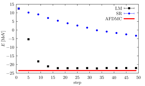
Figure 1: (Color online) Convergence pattern of the ⁴He variational energy at physical pion mass and $\Lambda=4$ fm ^-1 as a function of the number of optimization steps for the SR method (black squares) and the LM (blues circles). For comparison, the red line indicates the AFDMC result.

4 Results

With LO EFT($\not{\pi}$) LECs determined from experiment or LQCD calculations, predictions can be made with AFDMC for the binding energies of ⁴He and ¹⁶O.

In Table 1 we report results of ⁴He energies for all the values of the cutoff and of the pion mass we considered. Despite the different parametrization of the variational wave functions, the results are in very good agreement with those reported in Ref. [7], where a simplified version of the variational wave function was used because the LM had not been introduced yet. For most cutoff values, our results also agree with those of Ref. [9], which were obtained with the Resonating-Group and Hyperspherical-Harmonic methods. For $\Lambda\leq 6~{}\text{fm}^{-1}$, the QMC results differ by less than 0.1 MeV from Ref. [9], while for $\Lambda=8~{}\text{fm}^{-1}$ the QMC method binds ⁴He more deeply by more than 1 MeV. In consequence, the extrapolated asymptotic values differ. Our results display a better convergence pattern with the cutoff. At the physical pion mass and with the same input observables, our highest-cutoff result is in good agreement with the highest-cutoff result (cutoff values in the range $8-10$ fm^-1, but a different regulator function) of Ref. [14].

$\Lambda$	$m_{\pi}=140$ MeV	$m_{\pi}=510$ MeV	$m_{\pi}=805$ MeV
$2$ fm-1	$-23.17\pm 0.02$	$-31.15\pm 0.02$	$-88.09\pm 0.01$
$4$ fm-1	$-23.63\pm 0.03$	$-34.88\pm 0.03$	$-91.40\pm 0.03$
$6$ fm-1	$-25.06\pm 0.02$	$-36.89\pm 0.02$	$-96.97\pm 0.01$
$8$ fm-1	$-26.04\pm 0.05$	$-37.65\pm 0.03$	$-101.72\pm 0.03$ a
$\rightarrow\infty$	$-30_{\pm 2\,\text{(stat)}}^{\pm 0.3\,\text{(sys)}}$	$-39_{\pm 2\,\text{(stat)}}^{\pm 1\,\text{(sys)}}$	$-124_{\pm 1\,\text{(stat)}}^{\pm 3\,\text{(sys)}}$
Exp.	$-28.30$	–	–
LQCD	–	$-43.0\pm 14.4$	$-107.0\pm 24.2$

Table 1: ⁴He energy for different values of the pion mass $m_{\pi}$ and the cutoff $\Lambda$, compared to experiment and LQCD calculations [1, 2]. See main text and appendix for details on errors and extrapolations.

We found that an expansion of the type (3) up to $1/\Lambda^{2}$ suffices to extrapolate the ⁴He energies for $m_{\pi}=140$ MeV, since the addition of a cubic term changes neither the extrapolated value nor the best-fit coefficients. For the unphysical pion masses, the usage of the smallest cutoff is questionable because $\Lambda=2$ fm^-1 cuts off momentum modes below the pion mass. We thus extrapolate the values appearing in the tables with the quadratic expansion in Eq. (3) but without the result at $\Lambda=2$ fm^-1. In all cases, we perform fits with and without the $\Lambda=2$ fm^-1 results to estimate the systematic extrapolation error. The procedure adopted for the systematic and statistical errors quoted throughout this paper is detailed in the appendix.

It has to be remarked that this cutoff sensitivity study does not account for the EFT truncation error. Using cutoff variation from cutoff values somewhat larger than the pion mass, for example from $\Lambda=2$ fm^-1, 4 fm^-1, and 6 fm^-1 for $m_{\pi}=140$, $510$, and $805$ MeV, we might estimate the error as $\pm 7$, $\pm 4$, and $\pm 30$, respectively. Except for the intermediate pion mass, this is consistent with the rougher dimensional-analysis estimate $Q_{A}/M\sim 0.3$. In any case, we expect the truncation error to dominate over the statistical and extrapolation errors.

Given the convergence of the ⁴He binding energy with increasing cutoff, we confirm that, for both physical [14] and unphysical [7, 9] pion masses, LO EFT($\not{\pi}$) is renormalized correctly without the need for a four-nucleon interaction. In the physical case, the binding energy is underestimated for all values of the cutoff we considered, but the extrapolated value is in agreement with experiment even if we neglect the truncation error. Of course when the latter is taken into account we must conclude that such a good agreement is somewhat fortuitous. We expect NLO corrections, including Coulomb and two-nucleon effective-range corrections, to change the result by a few MeV. For $m_{\pi}=510$ MeV and $m_{\pi}=805$ MeV, our results reproduce LQCD predictions (where Coulomb is absent) within the measurement error over the entire cutoff range. As pointed out in Refs. [7, 9], this is a non-trivial consistency check: if either LQCD data or EFT($\not{\pi}$) were too wrong, one would expect no such agreement. However, LQCD uncertainties are too large at this point for us to draw a very strong conclusion.

It is interesting to study the cutoff dependence of the root-mean-square (rms) point-nucleon radius $\sqrt{\smash[b]{\langle r^{2}_{\text{pt}}\rangle}}$ and the single-nucleon point density $\rho_{\text{pt}}(r)$. These quantities are related to the charge density, which can be extracted from electron-nucleus scattering data, but are not observable themselves: few-body currents and single-nucleon electromagnetic form factors have to be accounted for. Still, one can gain some insight into the features of the ground-state wave function by comparing results at different pion masses and cutoffs. Since neither $\sqrt{\smash[b]{\langle r^{2}_{\text{pt}}\rangle}}$ nor $\rho_{\text{pt}}(r)$ commute with the Hamiltonian, the desired expectation values on the ground-state wave function are computed by means of “mixed” matrix elements

$$\langle\Psi_{0}|\mathcal{O}|\Psi_{0}\rangle\approx 2\langle\Psi_{T}|\mathcal{O}|\Psi_{0}\rangle-\langle\Psi_{T}|\mathcal{O}|\Psi_{T}\rangle\,.$$ (19)

In the above equation $|\Psi_{0}\rangle$ is the imaginary-time evolved state of Eq. (4), while $|\Psi_{T}\rangle$ is the trial wave function constructed as in Eq. (5).

The results for the point-proton radius of ⁴He are reported in Table 2. (Since Coulomb is absent in our calculation, the point-nucleon and point-proton radii are the same.) In the physical case, the calculated radius is much smaller than the empirical value — that is, the value extracted from the experimental data of Ref. [30] accounting for the nucleon size, but neglecting meson-exchange currents. A similar result, $\sqrt{\smash[b]{\langle r^{2}_{\text{pt}}\rangle}}\approx 1$ fm was obtained by the authors of Ref. [31] using a local form of a chiral interaction. NLO and N²LO potentials in a chiral expansion based on naive dimensional analysis [3, 4, 5] bring theory into much closer agreement with the empirical value. Hence, sub-leading terms in the EFT($\not{\pi}$) expansion could play a relevant role, at least for physical values of the pion mass.

For unphysically large pion masses, where EFT($\not{\pi}$) is supposed to exhibit a faster convergence, the point-proton radius is smaller than at $m_{\pi}=140$ MeV. The value obtained for $m_{\pi}=510$ MeV indicates a spatial extent similar to the physical one, while ⁴He at $m_{\pi}=805$ MeV, in comparison, seems to be a much more compact object. This is consistent with the behavior of the single-nucleon point density, $\rho_{\text{pt}}$, displayed in Fig. 2. For all cutoff values, the density corresponding to $m_{\pi}=805$ MeV is appreciably narrower than that computed for $m_{\pi}=510$ MeV or $m_{\pi}=140$ MeV. Focusing on $\Lambda=8$ fm^-1, $\rho_{\text{pt}}$ has a maximum value of $11.0$ fm^-3 for $m_{\pi}=805$ MeV, while in the $m_{\pi}=510$ MeV and $m_{\pi}=140$ MeV cases the maximum values are $2.1$ fm^-3 and $2.2$ fm^-3, respectively.

$\Lambda$	$m_{\pi}=140$ MeV	$m_{\pi}=510$ MeV	$m_{\pi}=805$ MeV
$2$ fm-1	$1.374\pm.0.004$	$1.482\pm 0.003$	$0.898\pm 0.001$
$4$ fm-1	$1.203\pm 0.004$	$1.133\pm 0.003$	$0.699\pm 0.001$
$6$ fm-1	$1.109\pm 0.003$	$1.035\pm 0.002$	$0.609\pm 0.001$
$8$ fm-1	$1.054\pm 0.003$	$0.976\pm 0.001$	$0.542\pm 0.001$
$\rightarrow\infty$	$0.9_{\pm 0.2\,\text{(stat)}}^{\pm 0.008\,\text{(sys)}}$	$0.8_{\pm 0.1\,\text{(stat)}}^{\pm 0.04\,\text{(sys)}}$	$0.25_{\pm 0.06\,\text{(stat)}}^{\pm 0.05\,\text{(sys)}}$
“Exp.”	$1.45$	–	–

Table 2: ⁴He point-proton radius for different values of the pion mass $m_{\pi}$ and the cutoff $\Lambda$, compared to the empirical value extracted from Ref. [30] accounting for the finite nucleon size. See main text and appendix for details on errors and extrapolations.

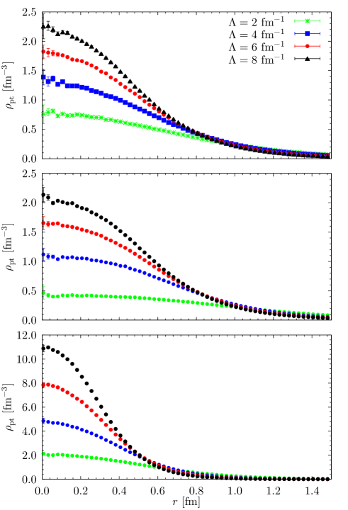
Figure 2: (Color online) ⁴He single-nucleon point density for $m_{\pi}=140$ MeV (upper panel), $m_{\pi}=510$ MeV (middle panel), and $m_{\pi}=805$ MeV (lower panel), at different values of the cutoff $\Lambda$.

The similarity between ⁴He ground-state properties at $m_{\pi}=510$ MeV and those at the physical pion mass exists despite differences in the structure of lighter systems. If confirmed for other properties of ⁴He and heavier nuclei, this semblance would mean that simulations at intermediate pion masses could provide useful insights into the physical world while saving substantial computational resources.

In Table 3 the ¹⁶O ground-state energies are reported for the same pion-mass and cutoff values considered for ⁴He. A striking feature is that ¹⁶O is not stable against breakup into four ⁴He clusters in almost all the cases, the only exception occurring for $m_{\pi}=140$ MeV and $\Lambda=2$ fm^-1, where ¹⁶O is $4.5$ MeV more bound than four ⁴He nuclei. In the other cases we miss the four-⁴He threshold by about $5$ MeV, which is beyond our statistical errors and reveals a lower bound on the systematic error of our QMC method.

$\Lambda$	$m_{\pi}=140$ MeV	$m_{\pi}=510$ MeV	$m_{\pi}=805$ MeV
$2$ fm-1	$-97.19\pm 0.06$	$-116.59\pm 0.08$	$-350.69\pm 0.05$
$4$ fm-1	$-92.23\pm 0.14$	$-137.15\pm 0.15$	$-362.92\pm 0.07$
$6$ fm-1	$-97.51\pm 0.14$	$-143.84\pm 0.17$	$-382.17\pm 0.25$
$8$ fm-1	$-100.97\pm 0.20$	$-146.37\pm 0.27$	$-402.24\pm 0.39$
$\rightarrow\infty$	$-115_{\pm 8\,\text{(stat)}}^{\pm 1\,\text{(sys)}}$	$-151_{\pm 10\,\text{(stat)}}^{\pm 2\,\text{(sys)}}$	$-504_{\pm 12\,\text{(stat)}}^{\pm 20\,\text{(sys)}}$
Exp.	$-127.62$	–	–

Table 3: ¹⁶O energy for different values of the pion mass $m_{\pi}$ and the cutoff $\Lambda$, compared with experiment. (No LQCD data exist for this nucleus.) See main text and appendix for details on errors and extrapolations.

Even considering only statistical and extrapolation errors the asymptotic values of the ¹⁶O energy cannot be separated from the four-⁴He threshold. The proximity of the threshold suggests that the structure of our ¹⁶O should be clustered. Indeed, despite no explicit clustering being enforced in the trial wave function, the highly efficient optimization procedure arranges the two- and three-body Jastrow correlations, as well as the orbital radial functions, in such a way as to favor configurations characterized by four independent ⁴He clusters.

The single-proton density profiles displayed in Fig. 3 indicate that only for $\Lambda=2$ fm^-1 with $m_{\pi}=140$ MeV and $m_{\pi}=510$ MeV are the nucleons distributed according to the classic picture of a bound wave function. For all the other combinations of pion masses and cutoffs, nucleons are pushed away from the center of the nucleus, which is basically empty — the density at the origin is a minuscule fraction of the peak — until $\simeq 2$ fm from the center of mass. The erratic behavior of the peak position of the density profiles as a function of the cutoff has to be ascribed to the fact that the relative position of the four ⁴He clusters is practically unaffected by the cutoff value. In fact, once the clusters are sufficiently apart, a landscape of degenerate minima in the variational energy emerges. Hence, the single-proton densities correspond to wave functions that, despite potentially significantly different, lead to almost identical variational energies. In contrast, the width of the peaks decreases with increasing cutoff in step with the shrinking of the individual ⁴He clusters reported in Table 2.

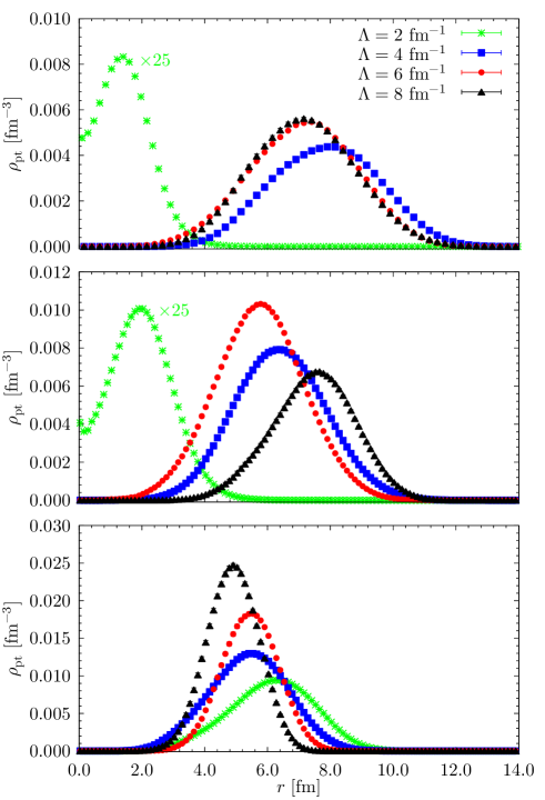
Figure 3: (Color online) ¹⁶O single-nucleon point density for $m_{\pi}=140$ MeV (upper panel), $m_{\pi}=510$ MeV (middle panel), and $m_{\pi}=805$ MeV (lower panel), at different values of the cutoff $\Lambda$.

The analysis of the proton densities alone does not suffice to support the claim of clustering. Another indication of clusterization comes from comparing the expectation values of the nuclear potentials evaluated in the ground states of ¹⁶O and ⁴He. For instance, in the $m_{\pi}=140$ MeV and $\Lambda=8$ fm^-1 case it turns out that the expectation values of the ¹⁶O two- and three-body potentials are $\simeq 4.05$ and $\simeq 4.16$ times larger than the corresponding values for ⁴He. The same pattern is observed for all the combinations of pion mass and cutoff, except for $\Lambda=2$ fm^-1 with $m_{\pi}=140$ MeV and $m_{\pi}=510$ MeV. In particular, for $\Lambda=2$ fm^-1 and $m_{\pi}=140$ MeV, the expectation values of the two- and three-body potentials in ¹⁶O are $\simeq 4.65$ and $\simeq 6.14$ times larger than in ⁴He. This difference is a consequence of the fact that the number of interacting pairs and triplets is larger when clusterization does not take place.

To better visualize the clusterization of the wave function, in Fig. 4 we display the position of the nucleons following the propagation of a single walker for 5000 imaginary-time steps, corresponding to $\Delta\tau=0.125$ MeV^-1, printed every 10 steps. In the upper panel, concerning $m_{\pi}=140$ MeV and $\Lambda=2$ fm^-1, nucleons are not organized in clusters. In fact, during the imaginary-time propagation they diffuse in the region in which the corresponding single-nucleon density of Fig. 3 does not vanish. A completely different scenario takes place at the same pion mass when $\Lambda=8$ fm^-1: the nucleons forming the four ⁴He clusters remain close to the corresponding centers of mass during the entire imaginary-time propagation. This is clear evidence of clustering. It has to be noted that the relative position of the four clusters is not a tetrahedron. To prove this, for each configuration we computed the moment-of-inertia matrix as in Ref. [32]. If the ⁴He clusters were positioned at the vertices of a tetrahedron, diagonalization would yield only two independent eigenvalues. Instead, we found three distinct eigenvalues, corresponding to an ellipsoid — yet another indication of the absence of interactions among nucleons belonging to different ⁴He clusters.

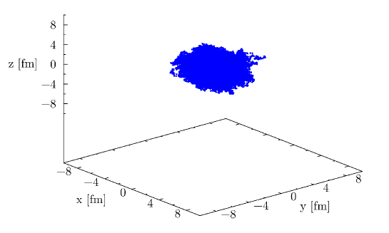
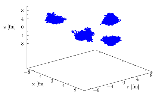
Figure 4: (Color online) Imaginary-time diffusion with time step $\Delta\tau=0.125$ MeV^-1 of a single walker for $m_{\pi}=140$ MeV, at $\Lambda=2$ fm^-1 (upper panel) and $\Lambda=8$ fm^-1 (lower panel).

The non-clustered states at $\Lambda=2~{}$fm^-1 for $m_{\pi}=510$ MeV and $m_{\pi}=140$ MeV deserve further comment. The state at $m_{\pi}=510$ MeV stands in contrast to the other states found above threshold whose structure is clustered. We interpret this as an artifact of the numerical method, since a perfect optimization procedure should have produced a clustered structure resembling the lower-energy state with four free ⁴He. While there is no signal of ¹⁶O stability above the physical pion mass, the state at $m_{\pi}=140$ MeV is certainly stable at the lowest cutoff, that is, when the interaction has the longest range. On this basis, one might speculate that at some pion mass above the physical one a transition from a non-clustered to a clustered state is expected. However, such a conclusion cannot be drawn until higher-order calculations in EFT($\not{\pi}$) — which will capture finer effects from pion exchange such as the tensor force at N²LO — are available.

The smaller relative size of the model space leads to more modest signs of cutoff convergence for ¹⁶O than ⁴He, which are reflected in larger extrapolation errors, especially at $m_{\pi}=805$ MeV. At physical pion mass, the central value of the extrapolated total energy is only 10% off experiment, which can be bridged by statistical and extrapolation errors. This difference is small compared to the expected truncation error, $\sim 30\%$. If there is a low-lying resonant or virtual state of ⁴He nuclei at LO in EFT($\not{\pi}$) — note that our analysis does neither preclude nor identify such a state — it is possible that the (perturbative) inclusion of higher-order terms up to N²LO will move the ¹⁶O energy sufficiently for stability with respect to four ⁴He clusters.

For unphysical pion mass, our results can be seen as an extension of LQCD to medium-mass nuclei, with no further assumptions about the QCD dynamics. In this case, a determination of the relative position of the four-⁴He threshold would further require much increased accuracy in the $A=2,3$ LQCD data that we use as input.

5 Conclusions

This paper represents the first application of the effective-field-theory formalism, as developed for small nuclei without explicit pions, to a relatively heavy object, ¹⁶O. We employed contact potentials which represent the leading order of a systematic expansion of QCD. This enabled us to analyze physical nucleons as well as simulated scenarios with increased quark masses.

To overcome the peculiar challenges associated with the solution of the Schrödinger equation, we have improved AFDMC by introducing a new optimization protocol of the many-body wave function to be employed in the variational stage of the calculation. The scheme we propose is an extension of the linear method and provides a much faster convergence in parameter space compared to stochastic reconfiguration, previously adopted in nuclear QMC calculations. Such accurate trial wave function is the starting point of the imaginary-time projection in AFDMC, which filters out the “exact” ground state of the Hamiltonian. This algorithm was used to predict not only ground-state energies, but also radii, densities, and particle distributions.

Our results for the ⁴He binding energy are in agreement with previous findings, including the renormalizability of the four-nucleon system in EFT($\not{\pi}$) without a LO four-body force. In particular, at physical pion mass the energy agrees with experiment within theoretical uncertainties. Moreover, the calculated point-nucleon radii and single-particle densities reveal a ⁴He structure at $m_{\pi}=510$ MeV similar to that at physical pion mass.

With this successful benchmark, we extended the calculations to ¹⁶O, obtaining extrapolated values for the ¹⁶O energy at all pion masses which are indistinguishable from the respective four-⁴He threshold, even considering only the smaller statistical and extrapolation errors. In fact, for almost all cutoffs and pion masses we considered, ¹⁶O is unstable with respect to break-up into four ⁴He nuclei. Our calculation of the ¹⁶O energy is the first time LQCD data are extended to the medium-mass region in a model-independent way .

Interestingly, $m_{\pi}=140$ MeV and $\Lambda=2$ fm^-1 is the only parameter set which yields a stable ¹⁶O. This suggests that the long-range structure of the interaction is deficient at larger cutoff values and might have to be corrected, e.g. via one-pion exchange, to guarantee the binding of heavier nuclei at LO. Alternatively, within a pionless framework, higher-order terms could act as perturbations to move ¹⁶O with respect to the four-⁴He threshold. At physical pion mass the central value of the total energy is just about 10% off experiment. This is only slightly larger than the statistical and extrapolation errors, and well within the $\sim 30\%$ truncation error estimate. We cannot exclude the possibility that agreement with data will improve with order. A comprehensive study of the various subsystems of ¹⁶O — for example, ¹²C, ⁸Be, and ⁴He-⁴He scattering — could determine whether a resonant or virtual shallow state at LO is transformed into a bound state by subleading interactions, thus elucidating the relation between clusterization and QCD.

In order to better appreciate the cluster nature of our solution for ¹⁶O, we have studied the radial nucleon density and the sampled probability density for the nucleons. In both cases the occurrence of clusterization is evident. From our results it is not possible to infer any significant correlation between the clusters, which once more confirms the extremely weak interaction among them within EFT($\not{\pi}$). We would like to point out that localization was not imposed in the wave function used to project out the ground state; rather, it spontaneously arises from the optimization procedure (despite the correlations being fully translationally invariant) and it is preserved by the subsequent imaginary-time projection.

Current QMC (AFDMC) results have now reached an accuracy level that allows for discussing the few-MeV energies involved in this class of phenomena, which are relevant for a deeper understanding of how the systematics in nuclear physics arises from QCD. Starting from LCQD data obtained for values of $m_{\pi}$ smaller than the ones employed in this work, and yet larger than the physical one, would allow us to establish the threshold for which nuclei as large as ¹⁶O are stable against the breakup into four ⁴He clusters, if such a threshold exists. To perform this analysis, it is essential to include higher-order terms in the EFT($\not{\pi}$) interaction, possibly up to N²LO, where tensor contributions appear. This also requires a substantial improvement of the existing LQCD data on light nuclei, which, even for large $m_{\pi}$, are currently affected by statistical errors that do not allow for an effective constraint of the interaction parameters.

Appendix: Statistical and systematic error estimation

The procedure we adopted in order to estimate the error in the extrapolations performed in this work is as follows. We can distinguish between two sources of errors. The first is a systematic error corresponding to the choice of neglecting the next (cubic) order in the expansion Eq. (3) and of removing the initial data point at $\Lambda=2$ fm^-1. The second is a statistical error coming from the uncertainties in the data used for the extrapolation.

The first kind of error is estimated by considering the maximum spread in three different extrapolations: two quadratic extrapolations obtained by either neglecting the results at $\Lambda=2$ fm^-1 or by using all available data (the latter is included only if the reduced $\chi^{2}$ is $\approx 1$) and a cubic extrapolation that uses all data.

For the second type of error, it is convenient to write Eq. (3) as a simple quadratic form,

$$\mathcal{O}_{\Lambda}=O+\mathcal{C}_{0}\Gamma+\mathcal{C}_{1}\Gamma^{2}+\cdots$$ (20)

where $\Gamma=1/\Lambda$. Given that we have only three pairs $(\Lambda,\mathcal{O}_{\Lambda})$, it is straightforward to see that

$$\mathcal{C}_{1}=\frac{1}{\Gamma_{2}-\Gamma_{3}}\left[\frac{\mathcal{O}_{2}-\mathcal{O}_{1}}{\Gamma_{2}-\Gamma_{1}}-\frac{\mathcal{O}_{3}-\mathcal{O}_{1}}{\Gamma_{3}-\Gamma_{1}}\right]$$ (21)

together with

$$\mathcal{C}_{0}=\frac{\mathcal{O}_{3}-\mathcal{O}_{1}}{\Gamma_{3}-\Gamma_{1}}-\left(\Gamma_{3}+\Gamma_{1}\right)\mathcal{C}_{1}$$ (22)

and

$$O=\mathcal{O}_{1}-\mathcal{C}_{0}\Gamma_{1}-\mathcal{C}_{1}\Gamma_{1}^{2}\;.$$ (23)

At this point it is simple to estimate the errors by propagation of the measurement uncertainty. We have

$$\delta\mathcal{C}_{1}=\frac{1}{\Gamma_{2}-\Gamma_{3}}\sqrt{\left[\frac{\delta\mathcal{O}_{2}^{2}+\delta\mathcal{O}_{1}^{2}}{\left(\Gamma_{2}-\Gamma_{1}\right)^{2}}+\frac{\delta\mathcal{O}_{3}^{2}+\delta\mathcal{O}_{1}^{2}}{\left(\Gamma_{3}-\Gamma_{1}\right)^{2}}\right]}$$ (24)

and

$$\delta\mathcal{C}_{0}=\sqrt{\frac{\delta\mathcal{O}_{3}^{2}+\delta\mathcal{O}_{1}^{2}}{\left(\Gamma_{3}-\Gamma_{1}\right)^{2}}+\left(\Gamma_{3}+\Gamma_{1}\right)^{2}\delta\mathcal{C}_{1}^{2}}\,,$$ (25)

and then finally

$$\delta O=\sqrt{\delta\mathcal{O}_{1}^{2}+\delta\mathcal{C}_{0}^{2}\Gamma_{1}^{2}+\delta\mathcal{C}_{1}^{2}\Gamma_{1}^{4}}\;.$$ (26)

Both error estimates appear in the results reported in the main text.

References

- [1] S. R. Beane, E. Chang, S. D. Cohen, W. Detmold, H. W. Lin, T. C. Luu, K. Orginos, A. Parreño, M. J. Savage, A. Walker-Loud, Light Nuclei and Hypernuclei from Quantum Chromodynamics in the Limit of SU(3) Flavor Symmetry, Phys. Rev. D87 (3) (2013) 034506. arXiv:1206.5219, doi:10.1103/PhysRevD.87.034506.
- [2] T. Yamazaki, K.-i. Ishikawa, Y. Kuramashi, A. Ukawa, Helium nuclei, deuteron and dineutron in 2+1 flavor lattice QCD, Phys. Rev. D86 (2012) 074514. arXiv:1207.4277, doi:10.1103/PhysRevD.86.074514.
- [3] P. F. Bedaque, U. van Kolck, Effective field theory for few nucleon systems, Ann. Rev. Nucl. Part. Sci. 52 (2002) 339–396. arXiv:nucl-th/0203055, doi:10.1146/annurev.nucl.52.050102.090637.
- [4] E. Epelbaum, H.-W. Hammer, U.-G. Meißner, Modern Theory of Nuclear Forces, Rev. Mod. Phys. 81 (2009) 1773–1825. arXiv:0811.1338, doi:10.1103/RevModPhys.81.1773.
- [5] R. Machleidt, D. R. Entem, Chiral effective field theory and nuclear forces, Phys. Rept. 503 (2011) 1–75. arXiv:1105.2919, doi:10.1016/j.physrep.2011.02.001.
- [6] K. E. Schmidt, S. Fantoni, A quantum Monte Carlo method for nucleon systems, Phys. Lett. B446 (1999) 99–103. doi:10.1016/S0370-2693(98)01522-6.
- [7] N. Barnea, L. Contessi, D. Gazit, F. Pederiva, U. van Kolck, Effective Field Theory for Lattice Nuclei, Phys. Rev. Lett. 114 (5) (2015) 052501. arXiv:1311.4966, doi:10.1103/PhysRevLett.114.052501.
- [8] S. R. Beane, E. Chang, W. Detmold, K. Orginos, A. Parreño, M. J. Savage, B. C. Tiburzi, Ab initio Calculation of the np→dγ Radiative Capture Process, Phys. Rev. Lett. 115 (13) (2015) 132001. arXiv:1505.02422, doi:10.1103/PhysRevLett.115.132001.
- [9] J. Kirscher, N. Barnea, D. Gazit, F. Pederiva, U. van Kolck, Spectra and Scattering of Light Lattice Nuclei from Effective Field Theory, Phys. Rev. C92 (5) (2015) 054002. arXiv:1506.09048, doi:10.1103/PhysRevC.92.054002.
- [10] J.-W. Chen, G. Rupak, M. J. Savage, Nucleon-nucleon effective field theory without pions, Nucl. Phys. A653 (1999) 386–412. arXiv:nucl-th/9902056, doi:10.1016/S0375-9474(99)00298-5.
- [11] X. Kong, F. Ravndal, Coulomb effects in low-energy proton proton scattering, Nucl. Phys. A665 (2000) 137–163. arXiv:hep-ph/9903523, doi:10.1016/S0375-9474(99)00406-6.
- [12] J. Vanasse, Fully Perturbative Calculation of Scattering to Next-to-next-to-leading-order, Phys. Rev. C88 (4) (2013) 044001. arXiv:1305.0283, doi:10.1103/PhysRevC.88.044001.
- [13] S. König, H. W. Grießhammer, H.-W. Hammer, U. van Kolck, Effective theory of 3H and 3He, J. Phys. G43 (5) (2016) 055106. arXiv:1508.05085, doi:10.1088/0954-3899/43/5/055106.
- [14] L. Platter, H.-W. Hammer, U.-G. Meißner, On the correlation between the binding energies of the triton and the alpha-particle, Phys. Lett. B607 (2005) 254–258. arXiv:nucl-th/0409040, doi:10.1016/j.physletb.2004.12.068.
- [15] I. Stetcu, B. R. Barrett, U. van Kolck, No-core shell model in an effective-field-theory framework, Phys. Lett. B653 (2007) 358–362. arXiv:nucl-th/0609023, doi:10.1016/j.physletb.2007.07.065.
- [16] B. Bazak, M. Eliyahu, U. van Kolck, Effective Field Theory for Few-Boson Systems, Phys. Rev. A94 (5) (2016) 052502. arXiv:1607.01509, doi:10.1103/PhysRevA.94.052502.
- [17] P. F. Bedaque, U. van Kolck, Nucleon deuteron scattering from an effective field theory, Phys. Lett. B428 (1998) 221–226. arXiv:nucl-th/9710073, doi:10.1016/S0370-2693(98)00430-4.
- [18] P. F. Bedaque, H.-W. Hammer, U. van Kolck, Effective theory of the triton, Nucl. Phys. A676 (2000) 357–370. arXiv:nucl-th/9906032, doi:10.1016/S0375-9474(00)00205-0.
- [19] U. van Kolck, Effective field theory of short range forces, Nucl. Phys. A645 (1999) 273–302. arXiv:nucl-th/9808007, doi:10.1016/S0375-9474(98)00612-5.
- [20] P. F. Bedaque, H.-W. Hammer, U. van Kolck, Renormalization of the three-body system with short range interactions, Phys. Rev. Lett. 82 (1999) 463–467. arXiv:nucl-th/9809025, doi:10.1103/PhysRevLett.82.463.
- [21] S. Binder, et al., Few-nucleon systems with state-of-the-art chiral nucleon-nucleon forces, Phys. Rev. C93 (4) (2016) 044002. arXiv:1505.07218, doi:10.1103/PhysRevC.93.044002.
- [22] J. Carlson, S. Gandolfi, F. Pederiva, S. C. Pieper, R. Schiavilla, K. E. Schmidt, R. B. Wiringa, Quantum Monte Carlo methods for nuclear physics, Rev. Mod. Phys. 87 (2015) 1067. arXiv:1412.3081, doi:10.1103/RevModPhys.87.1067.
- [23] S. Gandolfi, A. Lovato, J. Carlson, K. E. Schmidt, From the lightest nuclei to the equation of state of asymmetric nuclear matter with realistic nuclear interactions, Phys. Rev. C90 (6) (2014) 061306. arXiv:1406.3388, doi:10.1103/PhysRevC.90.061306.
-
[24]
S. Sorella, Wave
function optimization in the variational Monte Carlo method, Phys. Rev. B
71 (2005) 241103.
doi:10.1103/PhysRevB.71.241103.
URL http://link.aps.org/doi/10.1103/PhysRevB.71.241103 - [25] I. E. Lagaris, V. R. Pandharipande, Variational Calculations of Realistic Models of Nuclear Matter, Nucl. Phys. A359 (1981) 349–364. doi:10.1016/0375-9474(81)90241-4.
- [26] A. Arriaga, V. R. Pandharipande, R. B. Wiringa, Three body correlations in few body nuclei, Phys. Rev. C52 (1995) 2362–2368. arXiv:nucl-th/9506036, doi:10.1103/PhysRevC.52.2362.
- [27] J. Toulouse, C. J. Umrigar, Optimization of quantum Monte Carlo wave functions by energy minimization, J. Chem. Phys. 126 (8) (2007) 084102. arXiv:physics/0701039, doi:10.1063/1.2437215.
- [28] C. J. Umrigar, C. Filippi, Energy and variance optimization of many-body wave functions, Phys. Rev. Lett. 94 (2005) 150201. doi:10.1103/PhysRevLett.94.150201.
- [29] M. W. Lee, M. Mella, A. M. Rappe, Electronic quantum Monte Carlo calculations of atomic forces, vibrations, and anharmonicities, J. Chem. Phys. 122 (24) (2005) 244103. doi:10.1063/1.1924690.
- [30] C. R. Ottermann, G. Kobschall, K. Maurer, K. Rohrich, C. Schmitt, V. H. Walther, ELASTIC ELECTRON SCATTERING FROM HE-3 AND HE-4, Nucl. Phys. A436 (1985) 688–698. doi:10.1016/0375-9474(85)90554-8.
- [31] J. E. Lynn, J. Carlson, E. Epelbaum, S. Gandolfi, A. Gezerlis, A. Schwenk, Quantum Monte Carlo Calculations of Light Nuclei Using Chiral Potentials, Phys. Rev. Lett. 113 (19) (2014) 192501. arXiv:1406.2787, doi:10.1103/PhysRevLett.113.192501.
- [32] R. B. Wiringa, S. C. Pieper, J. Carlson, V. R. Pandharipande, Quantum Monte Carlo calculations of A = 8 nuclei, Phys. Rev. C62 (2000) 014001. arXiv:nucl-th/0002022, doi:10.1103/PhysRevC.62.014001.
- [33] C. McIlroy, C. Barbieri, T. Inoue, T. Doi, T. Hatsuda, Doubly magic nuclei from Lattice QCD forces at 469 MeV/c2arXiv:1701.02607.