Adaptive Filtering to Enhance Noise Immunity of Impedance/Admittance Spectroscopy: Comparison with Fourier Transformation

Abstract

The time domain technique for impedance spectroscopy consists in computing excitation voltage and current response Fourier images by fast or discrete Fourier transform and calculating their relation. Here we propose an alternative method for excitation voltage and current response processing for deriving system impedance spectrum based on fast and flexible adaptive filtering method. We show the equivalence between the problem of adaptive filter learning and deriving system impedance spectrum. To be specific we express the impedance via the adaptive filter weight coefficients. The noise canceling property of adaptive filtering has been also justified. Using the RLC circuit as a model system we experimentally show that adaptive filtering yields correct admittance spectra and elements ratings in the high noise conditions when Fourier transform technique fails. Providing the additional sensitivity for impedance spectroscopy, adaptive filtering can be applied to otherwise impossible to interpret time-domain impedance data. The advantages of adaptive filtering were justified with the practical living-cell impedance measurements.

I Introduction

Electrical immittance (impedance and admittance) spectroscopy Barsoukov and Macdonald (2005); Lvovich (2012) (EIS) is a powerful tool for electronic device diagnostics Lebedev Jr et al. (2000); Poklonski et al. (2010); Russell et al. (2010), materials characterization Berman and Lebedev (1981); Jacak et al. (1998); Lin et al. (2005); Arbi et al. (2005); Mesin and Scalerandi (2012); Das et al. (2015), electrochemistry Barbero and Lelidis (2007); Lelidis and Barbero (2005); Jorcin et al. (2006), alternative energy sources investigation Wang et al. (2013); Set et al. (2016); Tian et al. (2016); Rau et al. (2011), and experiments in biophysics Giaever and Keese (1993); Wegener et al. (2000); Grimnes and Martinsen (2015); Rivnay et al. (2015); Weckström et al. (1992); Jin et al. (2016). The research of a dynamic systems have become a hot topic of impedance spectroscopy in recent years. The excitation voltage (EV) with broad frequency spectrum like rectangular pulses, peaks, various types of noise, linear sweep or superposition of sine waves are commonly used for time resolved immittance spectroscopy. Employing such excitation signals allows scanning the sample in the wide frequency range, which gives significant advantage in performance and time resolution with respect to single-sine methods. To obtain the immittance spectrum (IS) from the collected data the fast/discrete Fourier transform (FFT/DFT) Brigham (1973); Rabiner and Gold (1975) of EV and current response is used Chang and Park (2010); Popkirov and Schindler (1992); Leisner et al. (2008). After which, the investigated system parameters are estimated by fitting the obtained IS with the complex nonlinear least squares method (CNLS) Macdonald and Garber (1977).

Obviously, the nature of dynamic and non-reversible systems does not allow experiment replication for data accumulation with the following statistical noise-canceling (averaging signal technique). To study them the technological improvements such as shielding, increasing EV, varying geometry of electrodes or low-noise electronics usage are required for increasing signal to noise ratio (SNR). If the sample produces its own noise or when the mentioned above methods are impractical, the obtained raw IS is distorted by noises and interferences, which complexifies data analysis. FFT does not provide the noise-canceling option by itself and thus the results of CNLS can be unreliable. For our best knowledge, only weighting method is currently used in this case for CNLS fit Barsoukov and Macdonald (2005); Lvovich (2012); Macdonald (1992). If this approach does not succeed, the IS data can not be interpreted and no information about the studied system can be gained.

The progressive signal processing methods (Kalman filtering Hamilton et al. (2016); Schütte et al. (2016), adaptive filtering Widrow and Stearns (1985), and other Rabiner and Gold (1975)) allows extraction more information from high noise data. The possibility of the adaptive filtering (AF) application for the IS processing has been previously noticed Wang et al. (2013). This approach can provide the solution of the problem mentioned above, due to the noise-canceling property of AF in the identification mode (learning) Widrow and Stearns (1985). Together with the usage of the broad frequency spectrum excitation signal, like in standard FFT method, decreasing the instrument influence on the sample and increasing time and frequency resolution Denda (1993, 1989); Chang and Park (2010); Popkirov and Schindler (1992); Leisner et al. (2008) as high as it is principally possible. In addition the AF requires relatively small computation power and available memory, which is important for on-line applications and creating portable devices. The information on IS is stored in weight coefficients (WC), decreasing memory requirement for IS data storage and to increasing IS data transfer speed. Finally, after filter learning phase, AF opens the direct way for creating the digital model resembling the behavior of the investigated system, which is useful for its further simulation.

Despite the successful application of the AF algorithm for the IS treatment in Ref. Wang et al. (2013), no theoretical background has been given for this approach and no comparison with other methods has been done. Present study is devoted to elucidation of these aspects.

In this paper we develop the theory of AF application for EIS. We analyze the relationship between the adaptive filter weight coefficients and the IS, derive the apparatus and weight functions of the AF method and theoretically justify its noise immunity. We experimentally show that the AF method is more accurate than the FFT, especially for high-noise raw data.

The paper is organized as follows. In subsection II.1 we introduce the AF model employed and in subsection II.2 we provide derivation of the system immittance on the basis of AF parameters, namely weight coefficients. In section III we describe the experimental setup for measuring immittance. In section IV on the basis of the obtained experimental data we justify the noise immunity property of AF with respect to FFT. In section V we demonstrate power of AF by its application for EIS-based in-vitro cell bio-sensing.

II Theory

II.1 Model

For processing the IS on the basis of AF method the investigated sample can be considered as a linear ”black-box” (Fig. 1).

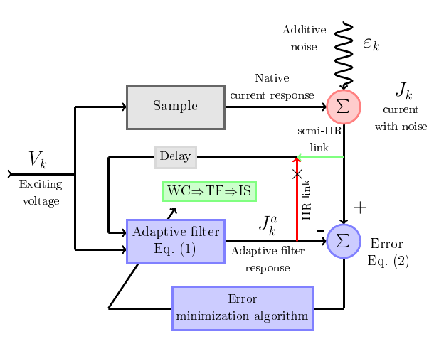
Figure 1: Processing the IS on the basis of AF method. Classical AF identification system with IIR corresponds for enabled IIR link (red) and disabled semi-IIR link (green), on the contrary this scheme describes semi-IIR model. If both links disabled, scheme describes FIR model.

The experimentally measured quantities are the exciting voltage $V_{k}$ being the input signal and current response $J_{k}$ being the output signal or in the terms of AF the desired signal. Index $k$ here is the time counter. The additive current noise $\varepsilon_{k}$ can also arise during measurements, due to the sample own noise, external noise or interfernces. We will now introduce $J_{k}^{a}$ as predictions of the adaptive filter:

$$J_{k}^{a}=\sum\limits_{j=1}^{\ell_{d}}d_{j}J_{k-j}^{a}+\sum\limits_{j=0}^{\ell_{n}}n_{j}V_{k-j},$$ (1)

where $d_{j}$ and $n_{j}$ are weight coefficients (WC), and the maximum value between $\ell_{d}$ and $\ell_{n}$ is the filtering order. So, Eq. (1) describes the causal (without loss of generality) discrete filter with infinite impulse response (IIR) Rabiner and Gold (1975). By adjusting the WC the following functional on the overall result of measurement is to be minimized

$$\sum\limits_{k=\max(\ell_{n},\ell_{d})}^{L}\left|J_{k}^{a}-J_{k}\right|^{2}=\min,$$ (2)

where $L+1$ is the total number of collected samples. The transfer function (TF) of Eq. (1) with the adjusted WC can be considered as an approximation of the sample admittance Wang et al. (2013) as it will be shown below in II.2.

It is well known, that the IIR filters are more flexible than the finite impulse response (FIR) filters. However the search of the WC values for IIR filters requires sufficient computation power and principal problem of the functional (2) local minimums exists Widrow and Stearns (1985). For increasing flexibility on the one hand, and for simplifying WC search on another hand, in this paper we introduce the ”semi-IIR” filter model. Namely, we replace in the right-hand part of Eq. (1) $J_{k}$ with $J_{k}^{a}$ before substituting it to Eq. (2). Thus the functional to be minimized takes a form

$$\sum_{k=\max(\ell_{n},\ell_{d})}^{L}\left|J_{k}-\sum_{j=1}^{\ell_{d}}d_{j}J_{k-j}-\sum_{j=0}^{\ell_{n}}n_{j}V_{k-j}\right|^{2}=\min.$$ (3)

Eq. (3) describes operating principle of AF with $V_{k}$ for input signal and $J_{k}$ for the desired response and for AF prediction simultaneously. Note that beginning of summation from $j=1$ for $d_{j}$ in Eq. (3) prevents the trivial solution $d_{0}=1$, $d_{j}=0$ when $j>0$ and $n_{j}=0$. The developed theory is also applicable for the FIR filters Wang et al. (2013) characterized by fixing $d_{j}=0$ and $\ell_{d}=0$, for the non-causal FIR and the non-causal ”semi”-IIR filter models.

II.2 The relation between time- and frequency domain

We shall now discuss the possibility of IS estimation with Eq. (3). For simplifying our analysis, we neglect measurement noise $\varepsilon_{k}$. If the sample rate $f_{0}$ is high enough one can change the summation by $k$ in Eq. (3) with integration over data collecting interval $[-T/2,T/2]$. On the basis of Parseval’s identity one can write the following

$$\int\limits^{T/2}_{-T/2}\left|J(t)-\sum_{j=1}^{\ell_{d}}d_{j}J(t-j\Delta t)-\sum_{j=0}^{\ell_{n}}n_{j}V(t-j\Delta t)\right|^{2}\operatorname{d}t=\\ =\int\limits^{+\infty}_{-\infty}\left|J(t)-\sum_{j=1}^{\ell_{d}}d_{j}J(t-j\Delta t)-\sum_{j=0}^{\ell_{n}}n_{j}V(t-j\Delta t)\right|^{2}\Pi\operatorname{d}t=\\ =2\pi\int\limits^{+\infty}_{-\infty}\left|\left(1-\sum\limits_{j=1}^{\ell_{d}}d_{j}\varphi_{j}\right)J(f)-V(f)\sum_{j=0}^{\ell_{n}}n_{j}\varphi_{j}\right|^{2}*K\operatorname{d}f,$$ (4)

where $\Pi$ is rectangle function in the interval $[-T/2,T/2]$, with Fourier image given by $\operatorname{sinc}$ function

$$K=\frac{\sin(\pi fT)}{\pi f},$$ (5)

$\varphi_{j}(f)=\exp[2\pi i\cdot j(f/f_{0})]$ is the Fourier image of the impulse delayed by $\Delta t=1/f_{0}$, $f$ is the frequency, asterisk $*$ denotes convolution, $V(f)$ and $J(f)$ are Fourier images of voltage and current, respectively. Now we use Ohm’s law $J(f)=YV(f)$, where $Y$ is admittance of the system at frequency $f$, and omit $2\pi$ multiplier. Thus from (4) one can write for the functional to be minimized:

$$\int\limits^{+\infty}_{-\infty}\left[\left|\left(1-\sum\limits_{j=1}^{\ell_{d}}d_{j}\varphi_{j}\right)Y-\sum_{j=0}^{\ell_{n}}n_{j}\varphi_{j}\right|^{2}\right.\\ \left.\vphantom{\left(1-\sum\limits_{j=1}^{\ell_{d}}d_{j}\varphi_{j}\right)}\times|V(f)|^{2}\right]*K\operatorname{d}f=\min.$$ (6)

Let us analyze Eq. (6). It is simple to see that $K$ plays a role of the apparatus function, which defines the frequency resolution of the method $\Delta f$. The latter can be calculated as the distance between the first positive and the first negative roots of $K$, which can be estimated as

$$\Delta f=\frac{1}{T}.$$ (7)

If the data collection time $T$ is long enough, $K$ can be replaced with the $\delta$-function, which allows to omit the convolution in Eq. (6). Henceforth we take convolution into account only as restriction on frequency resolution.

In these assumptions the squared magnitude of the EV image $|V(f)|^{2}$ is the weight function. Variation of its shape gives the possibility to control the influence of the selected frequency ranges on the IS processing.

According to Kotelnikov’s theorem, the condition $\operatorname{\textit{f}_{\mbox{\tiny B}}}\leq f_{0}/2$ must be met, where $\operatorname{\textit{f}_{\mbox{\tiny B}}}$ is the highest harmonic the exciting signal generator can produce. As a result, we obtain the following hierarchy of the characteristic setup frequencies:

$$\Delta f\ll\operatorname{\textit{f}_{\mbox{\tiny B}}}\leq f_{0}/2.$$ (8)

The most illustrative and practical is the case of exciting voltage with $|V(f)|=\operatorname{const}$ in the frequency band $f\leq\operatorname{\textit{f}_{\mbox{\tiny B}}}$. The excitation voltage types satisfying this condition are the white-noise, linear sweep and $\delta$-function signals. Thus Eq. (6) takes a form

$$\int\limits^{+\operatorname{\textit{f}_{\mbox{\tiny B}}}}_{-\operatorname{\textit{f}_{\mbox{\tiny B}}}}\left|\left(1-\sum\limits_{j=1}^{\ell_{d}}d_{j}\varphi_{j}\right)Y-\sum_{j=0}^{\ell_{n}}n_{j}\varphi_{j}\right|^{2}\operatorname{d}f=\min.$$ (9)

The integrand for case of IIR filter usage can be obtained by dividing the integrand in Eq. (9) by the squared absolute value of the expression in round brackets.

Eq. (9) is in fact the Levy approximation Levy (1959) for the admittnace $Y$ with $\varphi_{j}$ being the basis functions and one can write the following estimation of the admittance:

$$Y\approx\left(\sum_{j=0}^{\ell_{n}}n_{j}\varphi_{j}\right)\left/\left(1-\sum\limits_{j=1}^{\ell_{d}}d_{j}\varphi_{j}\right)\right..$$ (10)

One sees that the admittance $Y$ is directly derived on the basis of WC obtained by minimization of the functional in Eq. (3) with experimentally measured sequences of $V_{k}$ and $J_{k}$ substituted. AF method does not rely on FFT, which gives the advantage of memory economy. Since admittance estimation (10) is derived from Eq. (9) by heuristic manner, there are no obvious preference to use admittance $Y$ or impedance $Z=1/Y$ for IS analysis.

In the special case of FIR filter (denominator in Eq. (9) is equal to 1) together with additional condition $\operatorname{\textit{f}_{\mbox{\tiny B}}}=f_{0}/2$, WC $n_{j}$ are straightforwardly the Fourier coefficients of admittance. It means that any admittance, which can be expanded into Fourier series in the $\pm f_{b}$ interval (including ideal circuits and Warburg impedance) can be estimated by AF with any accuracy. In practice the most actual case is $f_{0}\gg\operatorname{\textit{f}_{\mbox{\tiny B}}}$. Thus for low enough AF order ($\ell_{d},\ell_{n}\ll f_{0}/\operatorname{\textit{f}_{\mbox{\tiny B}}}$) the $\varphi_{j}(f)$ arguments $2\pi i\cdot j(f/f_{0})$ are much less than 1. It means that the exponential functions $\varphi_{j}(f)$ can be expanded into the Taylor series and Eq. (10) becomes a rational function (standard Levy approximation) with coefficients being a linear combinations of $n_{j}$ and $d_{j}$.

Typically the admittances of real systems are given by rational functions or expandable into Taylor and Fourier series. However, the straight algebraic relation between the parameters of the studied system (the ratings of resistors, capacitors and inductors the system is formed of) and AF WC is complicated. Therefore we suggest using Eq. (10) for obtaining the frequency dependence of impedance. Due to the noise-cancelling property of AF, the yield of Eq. (10) can be considered as a noise-free approximation of real IS. Then the system parameters can be can be derived by applying the standard methods to the obtained IS: algebraic method (AM) Macdonald (1978), geometric methods Tsai and Whitmore (1982) or CNLS Macdonald and Garber (1977).

The procedure of functional (3) minimization and noise-canceling property of AF are discussed in appendices A and B, respectively.

III Experimental

The linear sweep-shape signal with 20 mV peak-to-peak amplitude, generated by signal generator AKIP-3413-3 (AKIP, Russia, 2 channels), was used as excitation voltage. The frequency range was from 10 Hz to 40 kHz and sweep time was 500 ms.

For $J_{k}$ measurements the ammeter (current-to-voltage converter) based on operational amplifier AD8606 (Analog Devices, USA) was assembled. It should be noticed that AD8606 has unity-gain frequency $f_{s}=10$ MHz and virtual inductance $L_{V}$ about several mH can arise due to the used back-feed resistor $R_{0}=100$ k$\Omega$. The corresponding equation reads as $L_{V}=R_{0}/(2\pi f_{s})$.

The L-Card E20-10 ADC (L-Card, Russia, 10 MHz band, 4 channels, 12 bit) was used in this study to record the exciting voltage $V_{k}$ and current response $J_{k}$ from the ammeter output. The data collection time $T$ was 500 ms and sampling rate $f_{0}=500$ kHz, which yields 250 thousands for the collected samples number. One sees that the experimental setup parameters obey the required frequencies hierarchy Eq.(8) and constant EV spectrum assumption (see apendix C). The setup scheme is shown on Fig. 2.

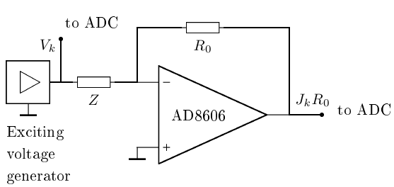
Figure 2: Setup for IS measurement using the time-domain technique. Operational amplifier is connected into current-to-voltage converter circuit. Here $Z$ is unknown sample impedance, $R_{0}$ is feed-back resistor.

The serial RLC-circuit was used as a sample. The multimeter DT9205A (Resanta, Russia) yields the reference values of circuit elements $C_{m}=10$ nF, $R_{m}=250$ $\Omega$, the inductance factory rating is 15 mH. The measurements were conducted with various signal to noise rations (SNR). For decreasing SNR the interference source (transformer connected to the generating white noise-shaped signal second channel of AKIP) was placed near the RLC-circuit. This is a simulation of the usual experimental practice: any electronic device (microscope, computer, display, motors, transformers and power electronic) located in close proximity to the sample produces interference. This method resemble e.g. an electrical biological cell-substrate impedance sensing (ECIS) device Wegener et al. (2000) or single cell EIS Dittami et al. (2008) with microscope control (see section V). SNR values were calculated as the relation between the noise-free $J_{k}$ std (EV output on, noise generator off) and the noise std (EV output off, noise generator output on).

To obtain lower values of SNR the simulation with digital artificial noise was conducted. The values $\varepsilon_{k}$ were generated by Matlab randn routine and added to current response $J_{k}$ obtained with the highest experimental SNR (30 dB). To achieve the statistics the data was collected over 4 experiments for each SNR for experimental and artificial digital noise.

To implement the AF-based derivation of IS the introduced above semi-IIR model with $\ell_{d}$=49 and $\ell_{n}=101$ was used. To obtain the IS with FFT the Fourier images of $V_{k}$ and $J_{k}$ were calculated in Matlab.

For further IS CNLS parameters fitting the Matlab code NELM based on Nelder-Mead simplex algorithm Lagarias et al. (1998) was written. The latter may be obtained from the authors. The freeware LEVM program Macdonald (1992) by Ross Macdonald and Origin package were not suitable for this purpose due to impossibility to process large input data set and support CUDA technology for decreasing run-time. Initial values of $R$, $L$, and $C$ for CNLS fit were 256 $\Omega$, 19.4 mH and 9.207 nF, respectively.

IV Results and discussion

The dependence of circuit element ratings CNLS fit on SNR for IS obtained by AF and FFT methods are presented on Fig. 4. In Fig. 3 the spectra and the corresponding CNLS fits for the 30 dB and the 3 dB SNR are shown. Corresponding CNLS fit results are listed in Table 1. One sees that AF-method is robust with respect to decreasing SNR.

SNR=30 dB                                               SNR=3 dB

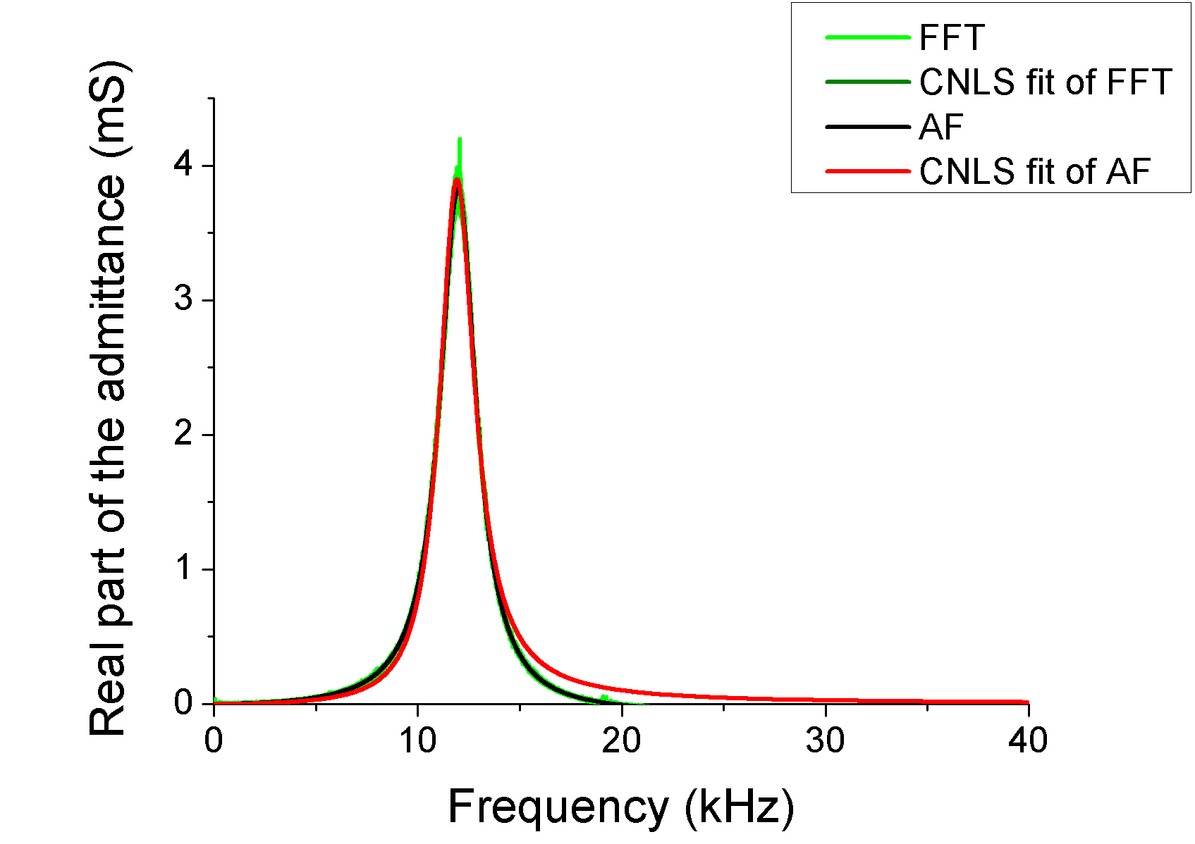
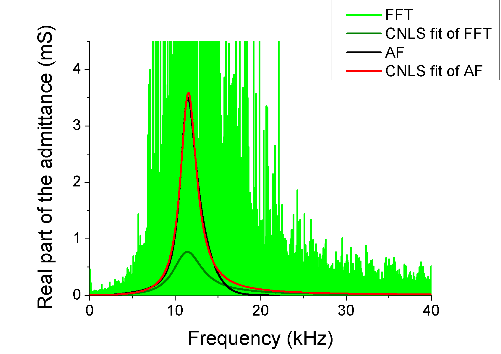
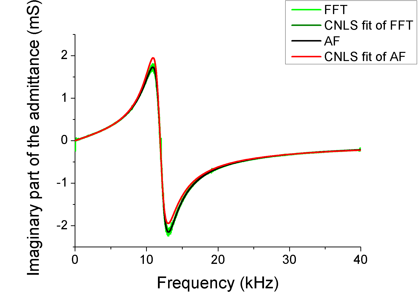
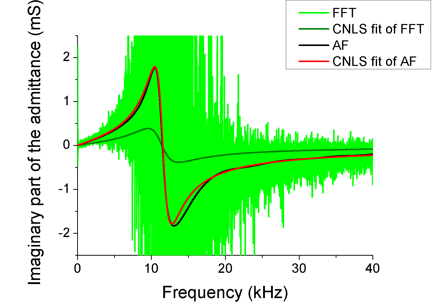
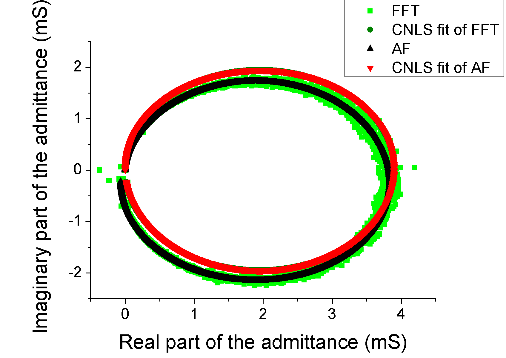
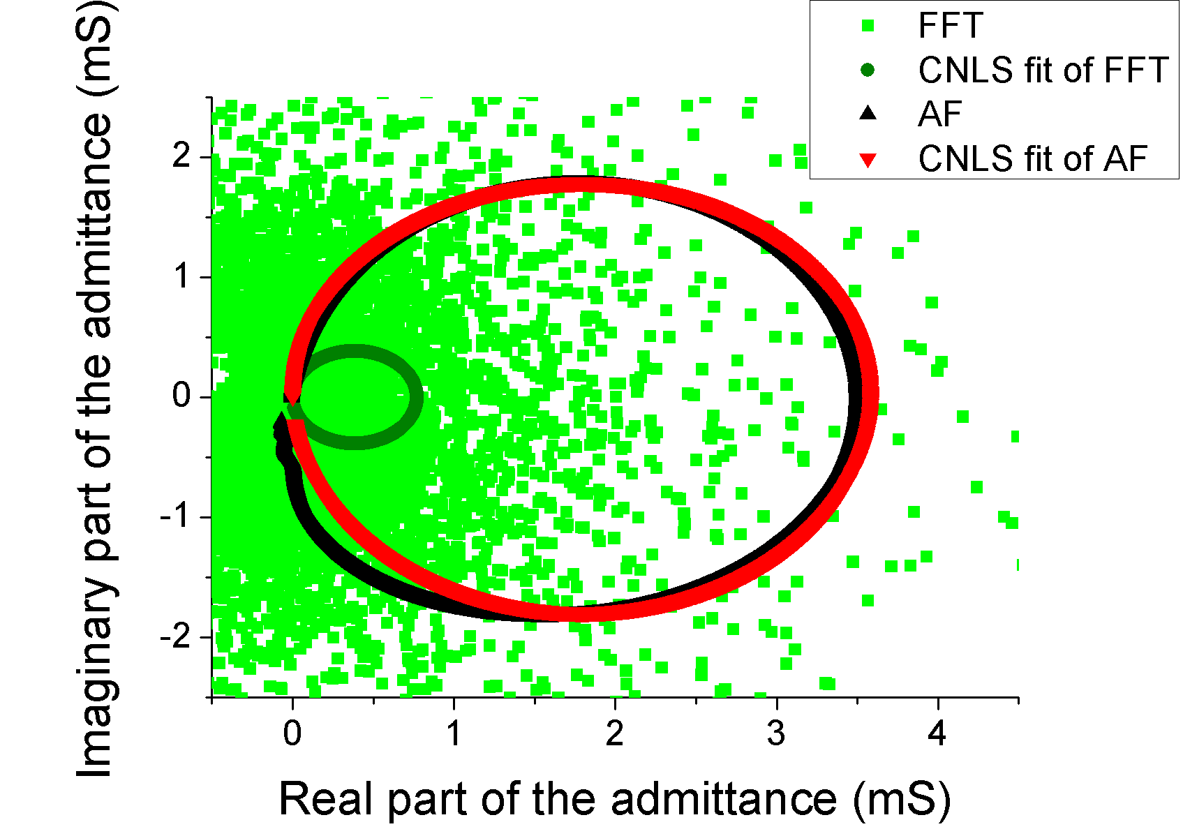
Figure 3: Frequency dependencies of admittance obtained with AF and FFT for the high and the low experimentally studied SNR. Panels (a), (c), and (e) correspond to SNR = 30 dB and show the admittance real and imaginary part spectra and the Nyquist plot, respectively. Panels (b), (d), (f) correspond to SNR = 3 dB. Light green color is used to show the raw admittance spectrum obtained by FFT and dark green color is used to show the CNLS fit of the corresponding spectra. The admittance spectra obtained by AF is shown with black color and its CNLS fit is shown by red color. The CNLS fits for AF and FFT on panels (a), (c), and (e) are overlapping.

Experiment                                     Simulation

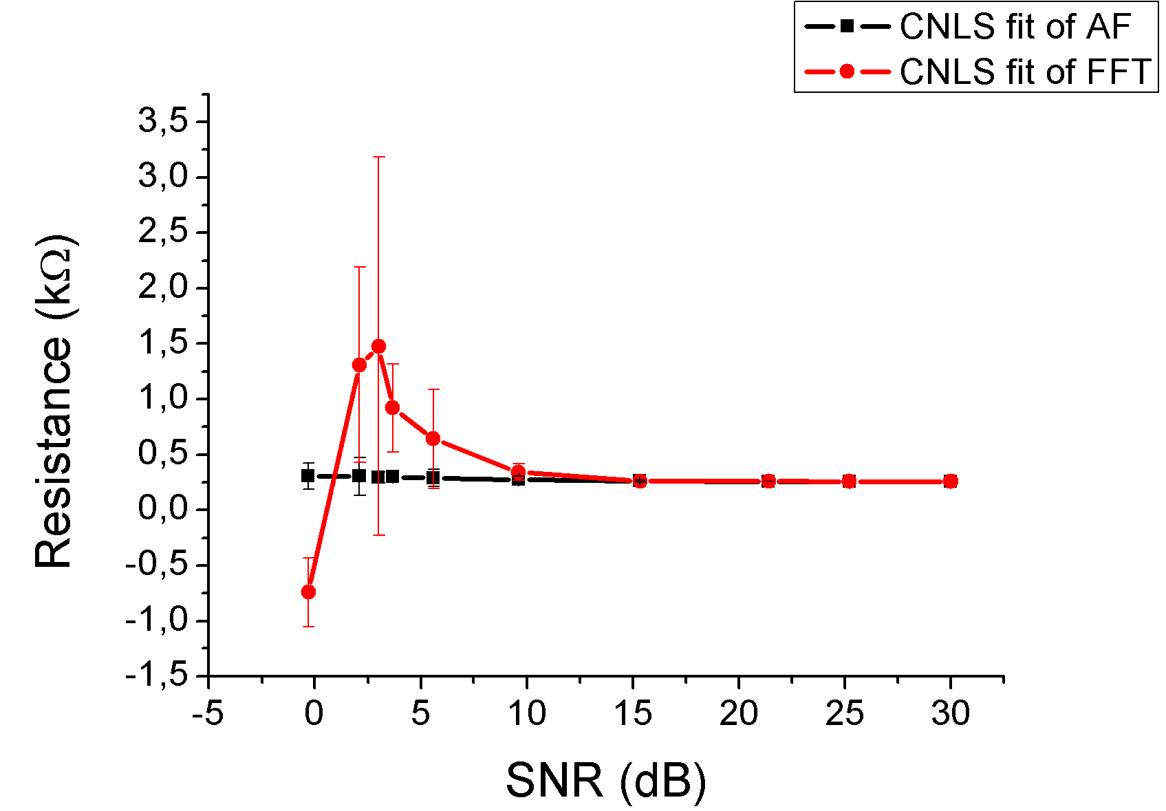
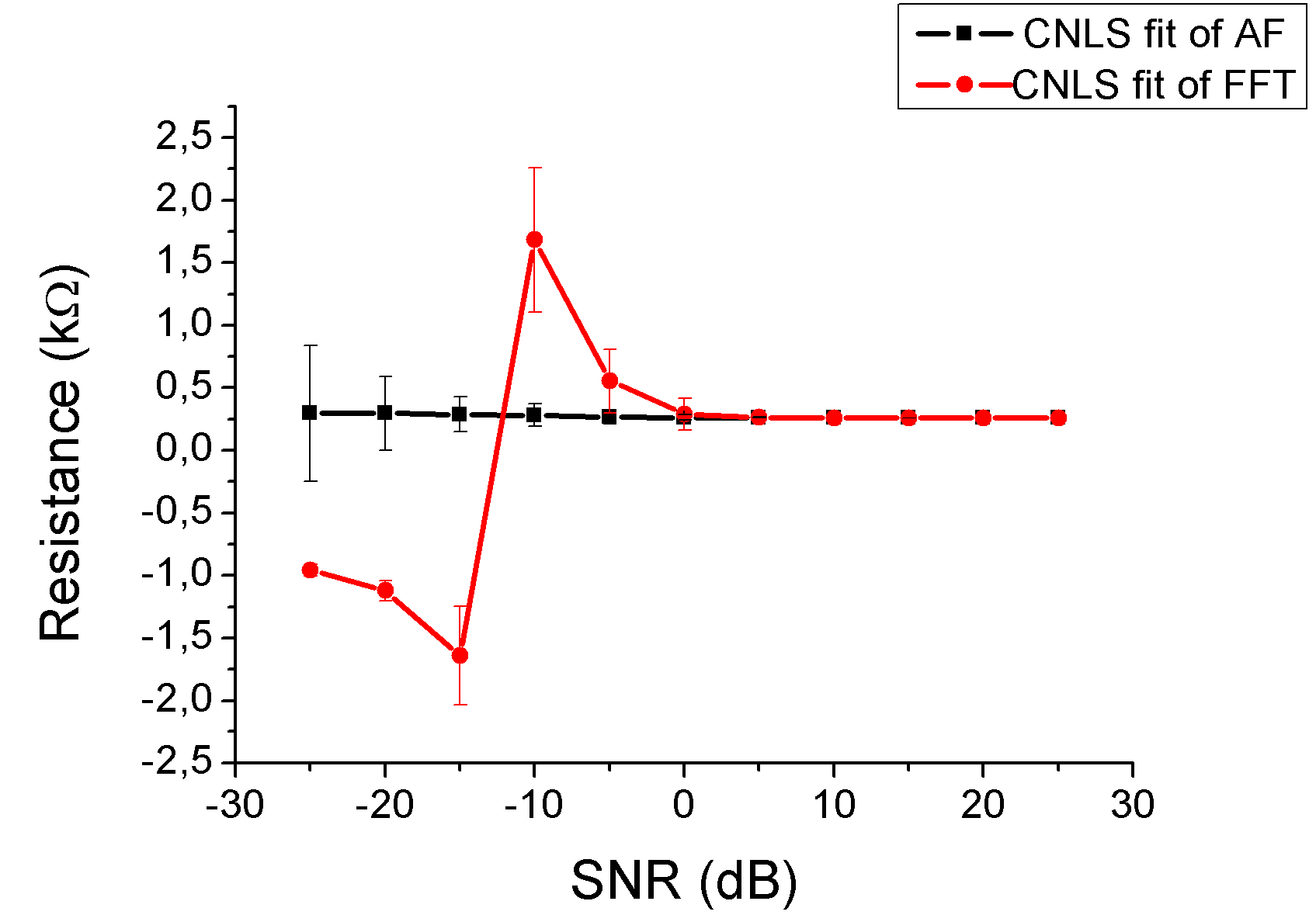
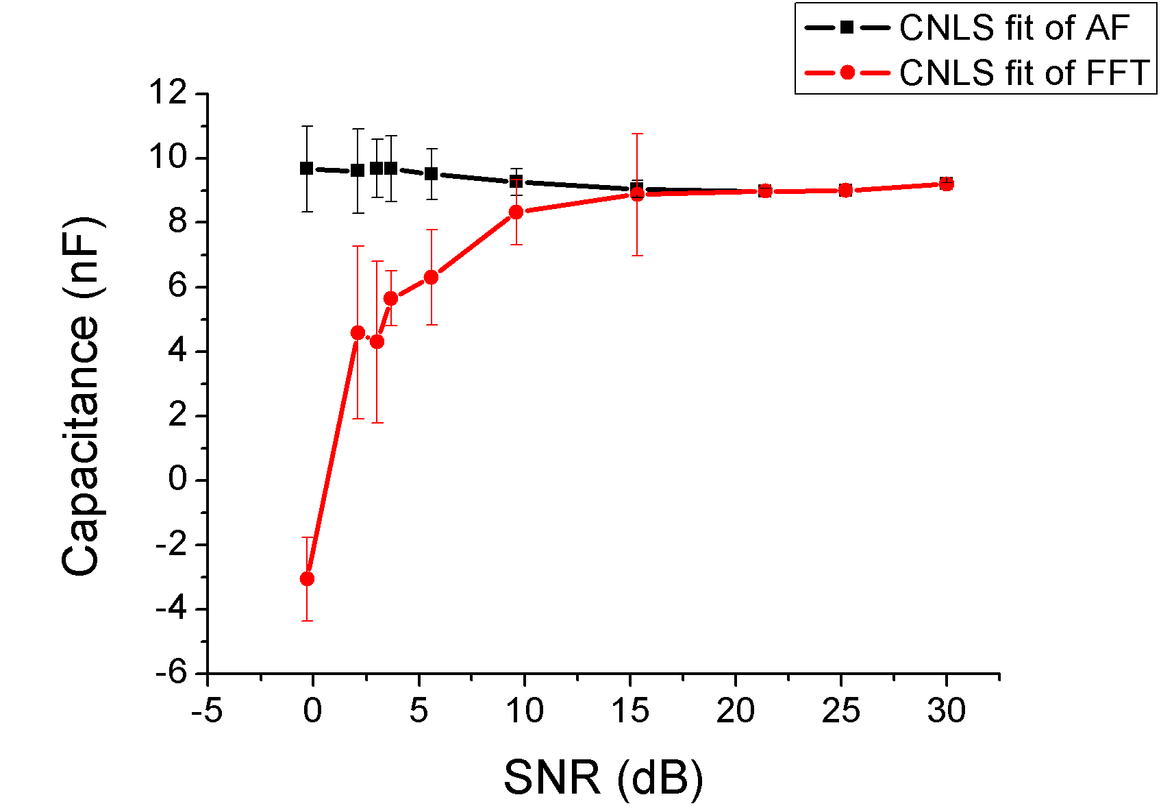
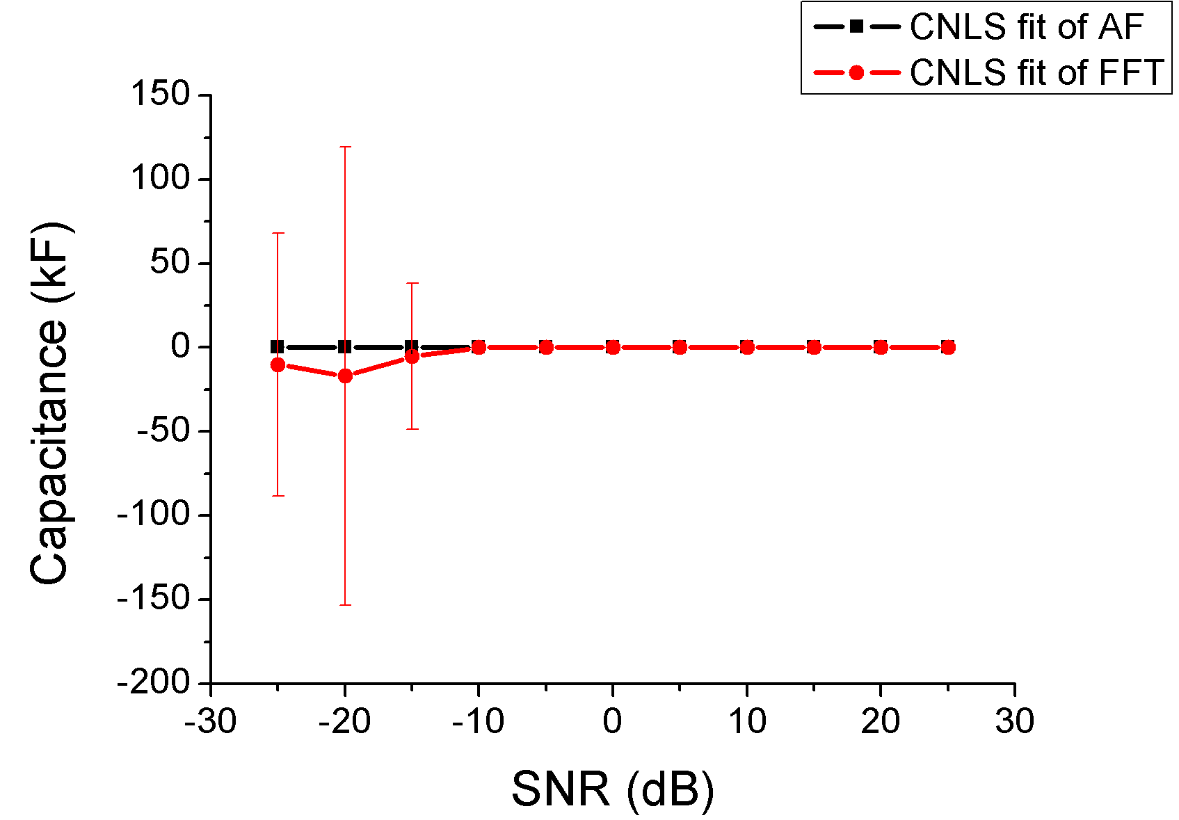
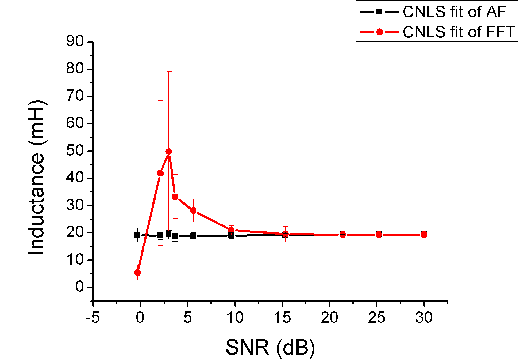
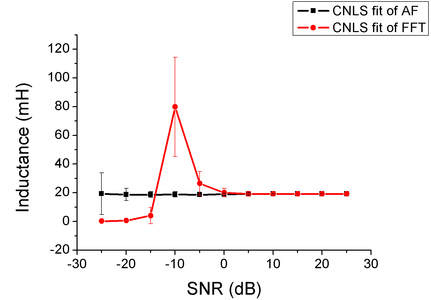
Figure 4: Dependence of the obtained circuit elements ratings on signal to noise ratio exhibiting the AF advances in noise immunity with respect to FFT. Black squares are for the results of CNLS fit of IS obtained by FFT. Red circles denote the circuit elements ratings obtained by AF. The statistics over 4 experiments for each SNR allows adding the error bars (99.9% reliability). Panels (a) and (c), (e) are for experimentally generated noise for resistance, capacitance and inductance, respectively. Panels (b), (d) and (f) are for digital artificial noise for resistance, capacitance and inductance, respectively. AF gives correct results for all studied SNR for both experimental noise and noise modeling. FFT fails at 5 dB for experimental data, and at 0 dB for noise modeling.

Table 1: RLC-circuit parameters estimation with 99.9% confidence intervals for different methods and SNRs. Last columns list the STD between CNLS fit of FFT yield and obtained with AF spectrum with respect to FFT.

SNR, dB	Method	$R$, $\Omega$	$C$, nF	$L$, mH	Residual type	Residual RMS, $\mu$S
30	AF $\&$ CNLS	$256.7\pm 0.4$	$9.209\pm 0.007$	$19.36\pm 0.02$	AF vs. FFT	30
	FFT $\&$ CNLS	$256.7\pm 0.3$	$9.207\pm 0.006$	$19.360\pm 0.007$	CNLS vs. FFT	110
3	AF $\&$ CNLS	$290\pm 50$	$9.7\pm 0.9$	$19\pm 2$	AF vs. FFT	3000
	FFT $\&$ CNLS	$1000\pm 2000$	$4\pm 3$	$50\pm 30$	CNLS vs. FFT	2000
30	AF $\&$ AM	$262.1\pm 0.4$	$9.37\pm 0.02$	$19.04\pm 0.04$	–
3		$300\pm 60$	$9\pm 1$	$21\pm 3$	–

At low SNR the spectra obtained by FFT are drastically distorted, which leads to incorrect estimation of $R$, $L$ and $C$ in CNLS fit. The FFT & CNLS fit fails at low SNR even in the case, where the correct ratings obtained at high SNR are used as initial fitting parameters. The discrepancy in capacitance value is especially high. No significant difference between unit, proportional, modulus and $|V(f)|^{2}$ weighting (see Table I in ref. Macdonald (1992)) on the FFT & CNLS fit results was observed. Contrary to FFT, the IS obtained by AF method do not degrade with SNR decreasing, and $R$, $L$ and $C$ ratings calculated from them stay intact. We relate this effect to the noise-canceling property of AF. Eliminating the uncorrelated with exciting voltage noise from IS prevents its influence on the circuit parameters estimation. Being the simplest artificial intelligence, AF automatically recognizes useful signal in the time domain data and separates it from the signal distorted by background noise.

It is not surprising that the confidence intervals (CI) of circuit elements ratings for both AF and FFT methods increase with decreasing SNR. For AF CI grow with decreasing SNR slower than in the case of FFT. Lower spectrum AF vs. FFT STD in the high SNR case is also not surprising because as can be seen from FFT data in Fig. 3 RLC-circuit IS is slightly distorted at high frequencies due to operational amplifier nonideality. AF semi-IIR model is more flexible than RLC-circuit model so the first one keeps this effect.

Interestingly, in the case of low SNR the residual error between IS obtained by FFT and the spectra obtained with AF is higher than that of FFT spectra and their CNLS fit. So, the least mean squares criterion is not adequate for low SNR and highly distorted IS. To the best of our knowledge, there is no proof of the CNLS noise immunity and present results ascertain this figure.

Smooth nature of the IS obtained by AF gives the possibility to use simple algebraic methods for circuit element ratings estimation, which gives significant advantage in computation power and eliminate human’s factor. For RLC circuit the elements ratings can be expressed via impedance magnitude minimum position frequency $f_{\min}$, impedance magnitude minimum value $|Z(f_{\min})|$, and frequency of the admittance imaginary part maximum position $f_{\max}$ as $R=|Z(f_{\min})|$, $L=Rf_{\max}/[2\pi(f_{\max}^{2}-f_{\min}^{2})]$ and $C=1/[L(2\pi f_{\min})^{2}]$. The results of AM fit are given in the last two rows of Table 1 for comparison with the results of CNLS. The element rating CI obtained by AM are not overlapped with CI for high SNR CNLS fits, because the AM use only few points from the IS at middle frequencies, and mentioned high-frequency systematic distortion (ADC nonideality) does not affect them.

V Practical example. Application for bio-sensors

In this section we present a practical example of bio-sensing, in which AF gives significant advantage with respect to FFT.

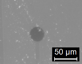
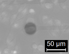
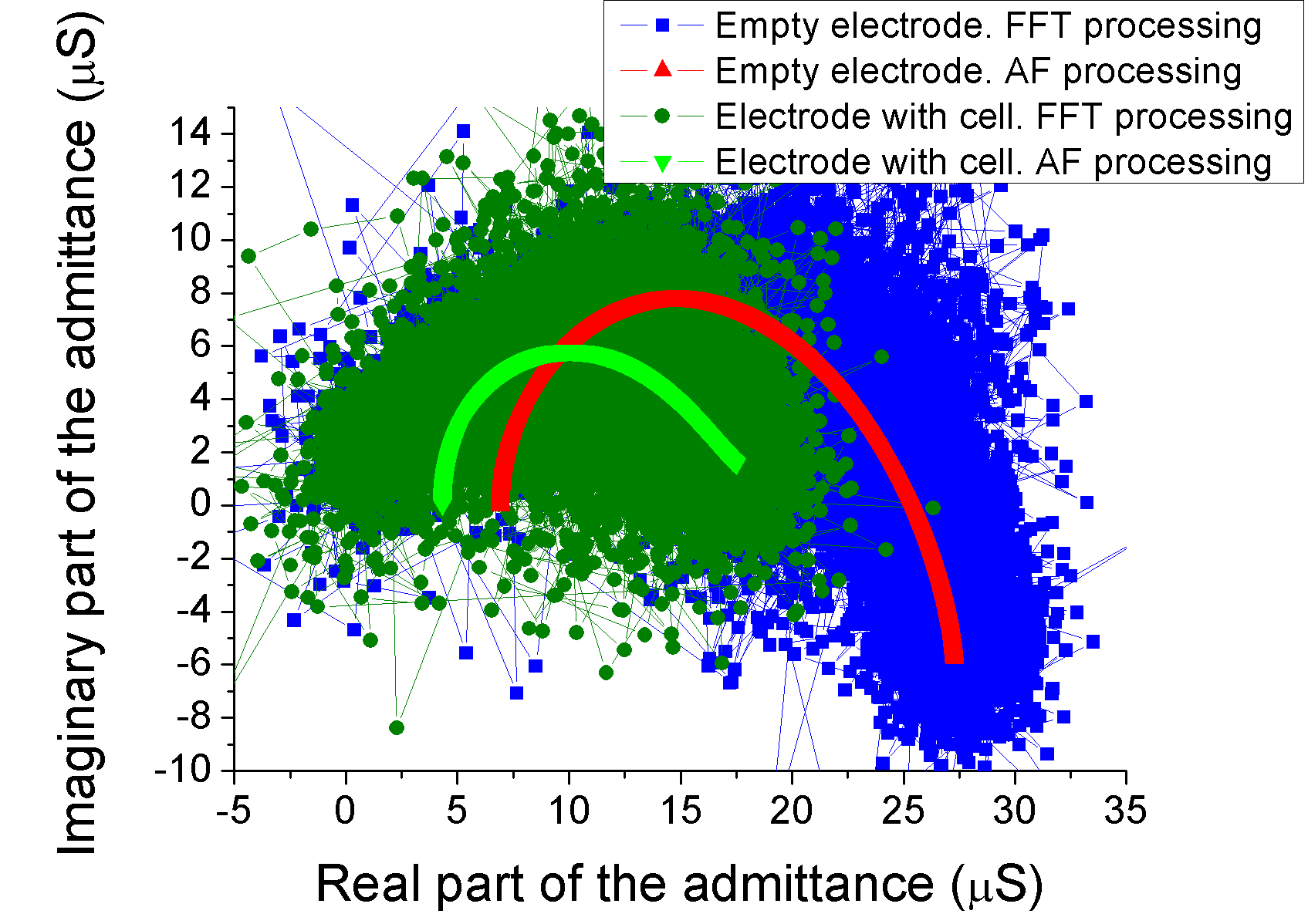
Figure 5: Application AF for bio-sensing EIS. (a) Empty electrode; (b) Electrode covered by cell. Diameter of electrodes is 30 $\mu$m; (c) Nyquist plot of obtained IS. Red and light green color denote the obtained by AF IS of the empty and the covered by cell electrodes, respectively. Blue and dark green color denote the obtained by FFT IS of the empty and the covered by cell electrodes, respectively. One sees that AF IS is more informative with respect to FFT IS, for example, it can be seen and agreement with Giaever-Keese model Wegener et al. (2000).

The investigated system was multielectrode array MEA 200/30 (Multi Channel Systems GmbH, Germany, 30 $\mu$m electrode diameter) covered by HeLa cells in phosphate buffered saline (Biolot, Russia) in vitro under microscope study. HeLa cells were obtained from the Bank of cell cultures of the Institute of Cytology of the Russian Academy of Sciences. IS was measured between large rectangle reference electrode (50 $\mu$m$\times 250\,\mu$m, not presented on photographs) and empty electrode (Fig. 5), and between reference electrode and electrode covered by a single cell (see Fig. 5). For IS measurement was used described above setup. Feedback resistor rating was 1 M$\Omega$, all other parameters was same as for RLC-circuit study. Results are presented on Fig. 5.

One can see, that IS obtained by FFT is distorted by interference from microscope, and no useful information can be achieved from it. Contrary, IS obtained by AF method is noise-free and more informative, for example, bright green and red arcs origins (their left ends) are displaced as predicted by Giaever-Keese model Wegener et al. (2000).

VI Conclusion and Outlook

In this study we have developed the theory of AF IS processing and compare this approach with FFT. The main outcome is that processing of time domain impedance data collected at low SNR conditions with FFT yields distorted and inadequate IS, but the IS obtained with AF method are robust with respect to noises even at negative SNR. The developed AF-based software for IS data processing can be obtained from the authors.

The developed AF-based approach makes impedance/admittance spectroscopy much more sensitive and brings it to the new level in all areas: material science, biophysics, electronic devices characterization and quality control in semiconductor industry. Moreover, the time domain impedance data ($V_{k}$ and $J_{k}$ sequences), which can not be interpreted with FFT approach, can be analyzed with AF-based one with higher probability of success.

This technique can find practical use in studying dynamic and nonreversible systems under the low SNR conditions. It is especially important for biological systems, because their investigation requires usage of the low excitation voltage and current, which results in decreasing of signal-noise ratio. Portable biosensors based on the developed method will be robust to the external interferences and noises. Moderate computation power and memory requirements also make AF appropriate for employing in this area.

Appendix A Functional minimization

On can see that Eq. (1) can be written in the terms of the Toeplitz matrices

$$L-\max(\ell_{n},\ell_{d})\left\{\vphantom{\begin{matrix}V_{\ell_{n}}&...&V_{2}&V_{1}&V_{0}\\ V_{\ell_{n}+1}&...&V_{3}&V_{2}&V_{1}\\ {5}\\ V_{\ell_{n}+r}&...&V_{r+2}&V_{r+1}&V_{r}\\ {5}\\ {5}\\ {5}\\ V_{L}&...&V_{L-\ell_{n}+1}&V_{L-\ell_{n}}&V_{L-\ell_{n}}\end{matrix}}\right.\left|\left|\overbrace{\begin{matrix}V_{\ell_{n}}&...&V_{2}&V_{1}&V_{0}\\ V_{\ell_{n}+1}&...&V_{3}&V_{2}&V_{1}\\ {5}\\ V_{\ell_{n}+r}&...&V_{r+2}&V_{r+1}&V_{r}\\ {5}\\ {5}\\ {5}\\ {5}\end{matrix}}^{\operatorname{\mbox{$\widehat{V}$}\hskip 2.27621pt}}\right|\right.\left.\left.\overbrace{\begin{matrix}J_{\ell_{d}}&...&J_{2}&J_{1}&J_{0}\\ J_{\ell_{d}+1}&...&J_{3}&J_{2}&J_{1}\\ {5}\\ J_{\ell_{d}+r}&...&J_{r+2}&J_{r+1}&J_{r}\\ {5}\\ {5}\\ {5}\\ {5}\end{matrix}}^{\operatorname{\mbox{$\widehat{J}$}\hskip 2.27621pt}}\right|\right|\cdot\overbrace{\begin{Vmatrix}n_{0}\\ n_{1}\\ n_{2}\\ ...\\ n_{\ell_{n}}\\ d_{1}\\ d_{2}\\ d_{3}\\ ...\\ d_{\ell_{d}}\end{Vmatrix}}^{\vec{w}}=\overbrace{\begin{Vmatrix}J_{\ell_{d}+1}\\ J_{\ell_{d}+2}\\ J_{\ell_{d}+3}\\ ...\\ J_{\ell_{d}+r}\\ ...\\ ...\end{Vmatrix}}^{\vec{J_{d}}},$$ (11)

where $\operatorname{\mbox{$\widehat{V}$}\hskip 2.27621pt}$ and $\operatorname{\mbox{$\widehat{J}$}\hskip 2.27621pt}$ is Toeplitz matrices generated by $V_{k}$ and $J_{k}$ sequences respectively, $\vec{w}$ is a vector obtained by $n_{j}$ and $d_{j}$ WC concatenation, and $\vec{J_{d}}$ is desired current response. In matrix notation the problem Eq. (3) takes a form

$$\left(\begin{Vmatrix}\operatorname{\mbox{$\widehat{V}$}\hskip 2.27621pt}\operatorname{\mbox{$\widehat{J}$}\hskip 2.27621pt}\end{Vmatrix}\vec{w}-\vec{J_{d}}\right)^{2}=\min$$ (12)

It is well known, that solution of the Eq. (12) can be reduced to solving the linear system

$$\begin{Vmatrix}\operatorname{\mbox{$\widehat{V}$}\hskip 2.27621pt}^{T}\\ \operatorname{\mbox{$\widehat{J}$}\hskip 2.27621pt}^{T}\end{Vmatrix}\begin{Vmatrix}\operatorname{\mbox{$\widehat{V}$}\hskip 2.27621pt}\operatorname{\mbox{$\widehat{J}$}\hskip 2.27621pt}\end{Vmatrix}\vec{w}=\begin{Vmatrix}\operatorname{\mbox{$\widehat{V}$}\hskip 2.27621pt}^{T}\\ \operatorname{\mbox{$\widehat{J}$}\hskip 2.27621pt}^{T}\end{Vmatrix}\vec{J_{d}}.$$ (13)

Thus the functional Eq.(3) minimization problem leads to the $(\ell_{n}+\ell_{d}+1)\times(\ell_{n}+\ell_{d}+1)$ linear system on vector $\vec{w}$ of WCs from which the admittance can be directly obtained with Eq. (10). To prevent any misunderstanding related with the existence of various physical dimensions in Eq. (13) we suggest the following normalization. The impedance $Z$ should be normalized to feedback resistor $R_{0}$ and all voltage inputs for ADC should be normalized to ADC range (see Fig. 2). This procedure makes all elements of $\operatorname{\mbox{$\widehat{V}$}\hskip 2.27621pt}$, $\operatorname{\mbox{$\widehat{J}$}\hskip 2.27621pt}$, $\vec{w}$, and $\vec{J_{d}}$ dimensionless.

Appendix B Noise immunity of AF

Now we will use normalization notation mentioned above and explain the noise-cancelling property of AF in the identification mode. To do so, we introduce the Toeplitz matrix $\operatorname{\mbox{$\widehat{\varepsilon}$}\hskip 2.27621pt}$ generated by current noise $\varepsilon_{k}$ sequence in the same manner as $\operatorname{\mbox{$\widehat{J}$}\hskip 2.27621pt}$ is generated by $J_{k}$ and add $\operatorname{\mbox{$\widehat{\varepsilon}$}\hskip 2.27621pt}$ to $\operatorname{\mbox{$\widehat{J}$}\hskip 2.27621pt}$. Thus Eq. (3) transforms to

$$\left(\begin{Vmatrix}\operatorname{\mbox{$\widehat{V}$}\hskip 2.27621pt}^{T}\operatorname{\mbox{$\widehat{V}$}\hskip 2.27621pt}&&\operatorname{\mbox{$\widehat{V}$}\hskip 2.27621pt}^{T}\operatorname{\mbox{$\widehat{J}$}\hskip 2.27621pt}\\ \operatorname{\mbox{$\widehat{J}$}\hskip 2.27621pt}^{T}\operatorname{\mbox{$\widehat{V}$}\hskip 2.27621pt}&&\operatorname{\mbox{$\widehat{J}$}\hskip 2.27621pt}^{T}\operatorname{\mbox{$\widehat{J}$}\hskip 2.27621pt}\\ \end{Vmatrix}+E_{L}\right)\vec{w}^{*}=\begin{Vmatrix}\operatorname{\mbox{$\widehat{V}$}\hskip 2.27621pt}^{T}\vec{J_{d}}\\ \operatorname{\mbox{$\widehat{J}$}\hskip 2.27621pt}^{T}\vec{J_{d}}\end{Vmatrix}+E_{R},$$ (14)

where

$$E_{L}=\begin{Vmatrix}0&&\operatorname{\mbox{$\widehat{V}$}\hskip 2.27621pt}^{T}\operatorname{\mbox{$\widehat{\varepsilon}$}\hskip 2.27621pt}\\ \operatorname{\mbox{$\widehat{\varepsilon}$}\hskip 2.27621pt}^{T}\operatorname{\mbox{$\widehat{V}$}\hskip 2.27621pt}&&\operatorname{\mbox{$\widehat{\varepsilon}$}\hskip 2.27621pt}^{T}\operatorname{\mbox{$\widehat{J}$}\hskip 2.27621pt}+\operatorname{\mbox{$\widehat{J}$}\hskip 2.27621pt}^{T}\operatorname{\mbox{$\widehat{\varepsilon}$}\hskip 2.27621pt}+\operatorname{\mbox{$\widehat{\varepsilon}$}\hskip 2.27621pt}^{T}\operatorname{\mbox{$\widehat{\varepsilon}$}\hskip 2.27621pt}\\ \end{Vmatrix},$$ (15)

$$E_{R}=\begin{Vmatrix}\operatorname{\mbox{$\widehat{V}$}\hskip 2.27621pt}^{T}\vec{\varepsilon}\\ \operatorname{\mbox{$\widehat{\varepsilon}$}\hskip 2.27621pt}^{T}\vec{J_{d}}+\operatorname{\mbox{$\widehat{J}$}\hskip 2.27621pt}^{T}\vec{\varepsilon}+\operatorname{\mbox{$\widehat{\varepsilon}$}\hskip 2.27621pt}^{T}\vec{\varepsilon}\\ \end{Vmatrix}$$ (16)

are perturbations, $\vec{w}^{*}$ is perturbed WC vector. If noise $\varepsilon$ is uncorrelated with EV and current then all products in $E_{R}$ and $E_{L}$ with $\operatorname{\mbox{$\widehat{V}$}\hskip 2.27621pt}$ and $\operatorname{\mbox{$\widehat{J}$}\hskip 2.27621pt}$ are equal to zero and perturbation depends only on the noise correlation function. Moreover, if noise is auto-correlated, then $E_{R}=0$ and $E_{L}$ is a diagonal matrix with $\ell_{d}$ non-zero elements. $L_{2}$-norm of $E_{L}$ in this case is noise mean square value $\langle\varepsilon^{2}\rangle$. In the basis of standard approach for linear system error estimation Verzbitskii (2007); Rice (1981); Golub and Loan (1996) one can write

$$\frac{|\vec{w}-\vec{w}^{*}|}{|\vec{w}|}\leq\frac{\langle\varepsilon^{2}\rangle\nu}{A},$$ (17)

where $\nu$ and $A$ are condition number and $L_{2}$-norm of main matrix in Eq.(13), respectively. The fact that $\langle\varepsilon^{2}\rangle$ is independent on the filtering order allows one to obtain the following estimation for root mean square of the relative error (RMSE) in WC from Eq.(17):

$$\mbox{RMSE}=\frac{1}{|\vec{w}|}\sqrt{\frac{\sum\limits_{j=0}^{\ell_{n}+\ell_{d}}(\vec{w}_{j}-\vec{w}^{*}_{j})^{2}}{\ell_{n}+\ell_{d}+1}}\leq\frac{\langle\varepsilon^{2}\rangle\nu}{A\sqrt{\ell_{n}+\ell_{d}+1}}.\\$$ (18)

In the most favorable case $\nu=1$ and RMSE of WC falls off as $1/\sqrt{\ell_{n}+\ell_{d}+1}$, which is a reminiscent of classical statistics law for signal averaging technique. If FIR model is used there are no influence of noise on WC (compare with ex. 6 on p. 226 in ref. Widrow and Stearns (1985)).

It should be noticed, that linear dependency of columns in $\begin{Vmatrix}\operatorname{\mbox{$\widehat{V}$}\hskip 2.27621pt}\operatorname{\mbox{$\widehat{J}$}\hskip 2.27621pt}\end{Vmatrix}$ leads to increasing of $\nu$ and, as corollary, to instability of the system (13). Such linear dependency can arise in the case of short periodic EV or in the case of pure resistance-type impedance. In this case for better robustness the singular value decomposition can be used directly for solving Eq.(11) Lawson and Hanson (1987).

Appendix C On the sweep-shape excitation voltage

The Fourier image of the linear sweep-shape signal is numerically investigated in Ref. Popkirov and Schindler (1992) (see Fig. 4(e)) and analytically obtained in the general form in Ref. Rozenberg (1982). By setting $r(t)$ in Eq. (9) in Ref. Rozenberg (1982) to rectangle function on sweep-time interval and by applying Eqs. 8.250.2-3 from ref. Gradshteyn and Ryzhik (2000) to result, we obtain difference between Frensel integrals, which is close to rectangle function on $\pm\operatorname{\textit{f}_{\mbox{\tiny B}}}$ interval.

References

- Barsoukov and Macdonald (2005) Evgenij Barsoukov and J. Ross Macdonald, Impedance Spectroscopy: Theory Experiment and Applications, 2nd ed. (Wiley-Interscience, 2005).
- Lvovich (2012) Vadim F. Lvovich, Impedance Spectroscopy: Applications to Electrochemical and Dielectric Phenomena, 1st ed. (Wiley, 2012).
- Lebedev Jr et al. (2000) A.A. Lebedev Jr, A.A. Lebedev, and D.V. Davydov, “Capacitance measurements for diodes in the case of strong dependence of the diode-base series resistance on the applied voltage,” Semiconductors 34, 115–118 (2000).
- Poklonski et al. (2010) N.A. Poklonski, N.I. Gorbachuk, S.V. Shpakovski, and A. Wieck, “Equivalent circuit of silicon diodes subjected to high-fluence electron irradiation,” Technical Physics 55, 1463–1471 (2010).
- Russell et al. (2010) K. J. Russell, F. Capasso, V. Narayanamurti, H. Lu, J. M. O. Zide, and A. C. Gossard, “Scattering-assisted tunneling: Energy dependence, magnetic field dependence, and use as an external probe of two-dimensional transport,” Phys. Rev. B 82, 115322 (2010).
- Berman and Lebedev (1981) L.S. Berman and A.A. Lebedev, Capacitance spectroscopy of deep levels (in russian) (Nauka, 1981).
- Jacak et al. (1998) Professor Lucjan Jacak, Dr. Arkadiusz Wojs, and Dr. Paweł Hawrylak, Quantum Dots, 1st ed., NanoScience and Technology (Springer-Verlag Berlin Heidelberg, 1998) Chap. 7, pp. 83–96.
- Lin et al. (2005) Yuanhua Lin, Lei Jiang, Rongjuan Zhao, and Ce-Wen Nan, “High-permittivity core/shell stuctured nio-based ceramics and their dielectric response mechanism,” Physical Review B 72, 014103 (2005).
- Arbi et al. (2005) K Arbi, M Tabellout, MG Lazarraga, JM Rojo, and J Sanz, “Non-arrhenius conductivity in the fast lithium conductor li 1.2 ti 1.8 al 0.2 (p o 4) 3: A li 7 nmr and electric impedance study,” Physical Review B 72, 094302 (2005).
- Mesin and Scalerandi (2012) Luca Mesin and Marco Scalerandi, “Effects of transducer size on impedance spectroscopy measurements,” Physical Review E 85, 051505 (2012).
- Das et al. (2015) Debanjan Das, Kumar Shiladitya, Karabi Biswas, Pranab Kumar Dutta, Aditya Parekh, Mahitosh Mandal, and Soumen Das, “Wavelet-based multiscale analysis of bioimpedance data measured by electric cell-substrate impedance sensing for classification of cancerous and normal cells,” Physical Review E 92, 062702 (2015).
- Barbero and Lelidis (2007) Giovanni Barbero and I Lelidis, “Evidence of the ambipolar diffusion in the impedance spectroscopy of an electrolytic cell,” Physical Review E 76, 051501 (2007).
- Lelidis and Barbero (2005) I Lelidis and Giovanni Barbero, “Effect of different anionic and cationic mobilities on the impedance spectroscopy measurements,” Physics Letters A 343, 440–445 (2005).
- Jorcin et al. (2006) Jean-Baptiste Jorcin, Mark E Orazem, Nadine Pébère, and Bernard Tribollet, “Cpe analysis by local electrochemical impedance spectroscopy,” Electrochimica Acta 51, 1473–1479 (2006).
- Wang et al. (2013) Shuoqin Wang, Mark Verbrugge, Luan Vu, Daniel Baker, and John S Wang, “Battery state estimator based on a finite impulse response filter,” Journal of The Electrochemical Society 160, A1962–A1970 (2013).
- Set et al. (2016) Ying Ting Set, Erik Birgersson, and Joachim Luther, “Predictive mechanistic model for the electrical impedance and intensity-modulated photocurrent and photovoltage spectroscopic responses of an organic bulk heterojunction solar cell,” Physical Review Applied 5, 054002 (2016).
- Tian et al. (2016) Jianjun Tian, Ting Shen, Xiaoguang Liu, Chengbin Fei, Lili Lv, and Guozhong Cao, “Enhanced performance of pbs-quantum-dot-sensitized solar cells via optimizing precursor solution and electrolytes,” Scientific reports 6 (2016).
- Rau et al. (2011) Uwe Rau, Daniel Abou-Ras, and Thomas Kirchartz, Advanced Characterization Techniques for Thin Film Solar Cells, 1st ed. (Wiley-VCH, 2011) Chap. 4, pp. 81–105.
- Giaever and Keese (1993) Ivar Giaever and Charles R Keese, “A morphological biosensor for mammalian cells.” Nature 366, 591 (1993).
- Wegener et al. (2000) Joachim Wegener, Charles R Keese, and Ivar Giaever, “Electric cell–substrate impedance sensing (ecis) as a noninvasive means to monitor the kinetics of cell spreading to artificial surfaces,” Experimental cell research 259, 158–166 (2000).
- Grimnes and Martinsen (2015) Sverre Grimnes and Orjan G. Martinsen, Bioimpedance and bioelectricity basics, 3rd ed. (Academic Press, , Elsevier Ltd, 2015).
- Rivnay et al. (2015) Jonathan Rivnay, Pierre Leleux, Adel Hama, Marc Ramuz, Miriam Huerta, George G Malliaras, and Roisin M Owens, “Using white noise to gate organic transistors for dynamic monitoring of cultured cell layers,” Scientific reports 5 (2015).
- Weckström et al. (1992) M Weckström, E Kouvalainen, and M Juusola, “Measurement of cell impedance in frequency domain using discontinuous current clamp and white-noise-modulated current injection,” Pflügers Archiv 421, 469–472 (1992).
- Jin et al. (2016) Seon-Ah Jin, Shishir Poudyal, Ernesto E Marinero, Richard J Kuhn, and Lia A Stanciu, “Impedimetric dengue biosensor based on functionalized graphene oxide wrapped silica particles,” Electrochimica Acta 194, 422–430 (2016).
- Brigham (1973) E. Oran Brigham, The fast Fourier transform: An introduction to its theory and application, prentice-hall ed. (Prentice Hall, 1973).
- Rabiner and Gold (1975) Lawrence R. Rabiner and Bernard Gold, Theory and Application of Digital Signal Processing (Prentice Hall, 1975).
- Chang and Park (2010) Byoung-Yong Chang and Su-Moon Park, “Electrochemical impedance spectroscopy,” Annual Review of Analytical Chemistry 3, 207–229 (2010).
- Popkirov and Schindler (1992) GS Popkirov and RN Schindler, “A new impedance spectrometer for the investigation of electrochemical systems,” Review of scientific instruments 63, 5366–5372 (1992).
- Leisner et al. (2008) Malte Leisner, Jürgen Carstensen, and Helmut Föll, “Fft impedance spectroscopy analysis of the growth of anodic oxides on (100) p-si for various solvents,” Journal of Electroanalytical Chemistry 615, 124–134 (2008).
- Macdonald and Garber (1977) J Ross Macdonald and JA Garber, “Analysis of impedance and admittance data for solids and liquids,” Journal of the Electrochemical Society 124, 1022–1030 (1977).
- Macdonald (1992) James Ross Macdonald, “Comparison and application of two methods for the least squares analysis of immittance data,” Solid State Ionics 58, 97–107 (1992).
- Hamilton et al. (2016) Franz Hamilton, Tyrus Berry, and Timothy Sauer, “Ensemble kalman filtering without a model,” Physical Review X 6, 011021 (2016).
- Schütte et al. (2016) Dirk Schütte, S. Z. Sayed Hassen, Kai S. Karvinen, Toby K. Boyson, Abhijit G. Kallapur, Hongbin Song, Ian R. Petersen, Elanor H. Huntington, and Michèle Heurs, “Experimental demonstration of frequency autolocking an optical cavity using a time-varying kalman filter,” Phys. Rev. Applied 5, 014005 (2016).
- Widrow and Stearns (1985) Bernard Widrow and Peter N. Stearns, Adaptive Signal Processing, Prentice-Hall signal processing series (Prentice-Hall, 1985).
- Denda (1993) W. Denda, Noise as source of information (in russian) (Mir, 1993) Chap. 6, pp. 135–150.
- Denda (1989) W. Denda, Rauschen als Information (in Deutsch) (Hüthig, 1989).
- Levy (1959) EC Levy, “Complex-curve fitting,” IRE transactions on automatic control , 37–43 (1959).
- Macdonald (1978) Digby D Macdonald, “A method for estimating impedance parameters for electrochemical systems that exhibit pseudoinductance,” Journal of the Electrochemical Society 125, 2062–2064 (1978).
- Tsai and Whitmore (1982) Y-T Tsai and DH Whitmore, “Nonlinear least-squares analyses of complex impedance and admittance data for solid electrolytes,” Solid State Ionics 7, 129–139 (1982).
- Dittami et al. (2008) Gregory M Dittami, H Edward Ayliffe, Curtis S King, and Richard D Rabbitt, “A multilayer mems platform for single-cell electric impedance spectroscopy and electrochemical analysis,” Journal of Microelectromechanical Systems 17, 850–862 (2008).
- Lagarias et al. (1998) Jeffrey C Lagarias, James A Reeds, Margaret H Wright, and Paul E Wright, “Convergence properties of the nelder–mead simplex method in low dimensions,” SIAM Journal on optimization 9, 112–147 (1998).
- Verzbitskii (2007) V. M. Verzbitskii, Computation linear algebra (in russian) (Visshay shkola, 2007) Chap. 8.3, pp. 307–313.
- Rice (1981) John R. Rice, Matrix Computations and Mathematical Software (McGraw-Hill Computer Science Series) (1981) Chap. 9.B, pp. 112–115.
- Golub and Loan (1996) H. Golub and Charles F. Van Loan, Matrix Computations, 3rd ed., Johns Hopkins studies in the mathematical sciences (Johns Hopkins University Press, 1996) Chap. 2.7.2, pp. 80–82, eq. 2.7.4.
- Lawson and Hanson (1987) Charles L. Lawson and Richard J. Hanson, Solving least squares problems, Classics in applied mathematics 15 (Society for Industrial and Applied Mathematics, 1987) Chap. 18, pp. 107–120.
- Rozenberg (1982) Maurice Rozenberg, “Linear sweep synthesis,” Computer Music Journal 6, 65–71 (1982).
- Gradshteyn and Ryzhik (2000) I. S. Gradshteyn and M. Ryzhik, Table of integrals, series, and products, 6th ed. (Academic Press, 2000) p. 880.