Identification of Unmodeled Objects from Symbolic Descriptions*

Abstract

Successful human-robot cooperation hinges on each agent’s ability to process and exchange information about the shared environment and the task at hand. Human communication is primarily based on symbolic abstractions of object properties, rather than precise quantitative measures. A comprehensive robotic framework thus requires an integrated communication module which is able to establish a link and convert between perceptual and abstract information.

The ability to interpret composite symbolic descriptions enables an autonomous agent to

operate in unstructured and cluttered environments, in tasks which involve unmodeled or never seen before objects; and

exploit the aggregation of multiple symbolic properties as an instance of ensemble learning, to improve identification performance even when the individual predicates encode generic information or are unprecisely grounded.

We propose a discriminative probabilistic model which interprets symbolic descriptions to identify the referent object contextually w.r.t. the structure of the environment and other objects. The model is trained using a collected dataset of identifications, and its performance is evaluated by quantitative measures and a live demo developed on the PR2 robot platform, which integrates elements of perception, object extraction, object identification and grasping.

I INTRODUCTION

The human ability to compose and interpret object descriptions is a fundamental one for the purpose of efficient collaboration during the concurrent multi-agent execution of a complex task. Humans are very skilled at guessing games in which they have to identify objects given sparse, incomplete or even mildly contradictory information. Succeeding at such guessing games generally requires two complementary skills: the ability to describe an object using a pre-specified language ( encoding the object identity), and the ability to identify an object given its description ( decoding the object identity). Both skills abstract the human ability to communicate about objects in a wide range of environments. As robotics research moves from passive single-agent tasks to active manipulation in close collaboration with humans, the ability to play such guessing games is bound to extend an autonomous system’s workspace.

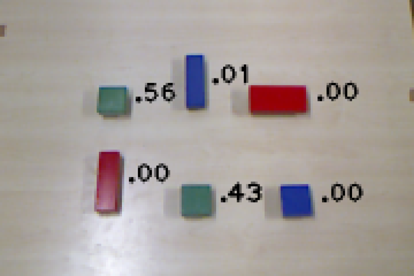
(A) at (0,0)[draw=black] ; [draw=black, below left=of A.south west, anchor=north] (B) ; [draw=black, below right=of A.south east, anchor=north] (C) ;

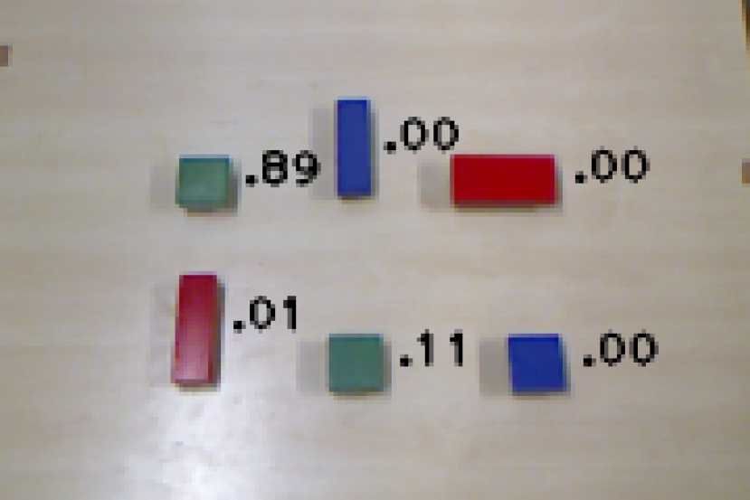
Figure 1: On the top, the identification distribution given an ambiguous description green. On the bottom left and right, the identification distributions for more specific descriptions, respectively green bottom and green left.

Humans share information and reason about objects using a symbolic language consisting of low- and high-level (relational) qualitative properties,  blue, laptop, next_to. These symbolic predicates can be flexibly composed into structured descriptions ( “Get the thin book next_to the white laptop”) which are typically tailored around the existing environment. The previous description might be suitable (or even redundant) for some environments, but ambiguous in others,  in rooms where there are many books and laptops. The modularity of such descriptions enables them to refer to an object which lacks a single prominent identifying quality, and to exploit groups of uncertain properties which still contribute to the overall identification process, in the style of ensemble models (front_page).

Concerning object recognition, a number of approaches are often used to overcome the hurdle of perception. Either the world is restricted to a predefined structure and degree of sparsity; or all objects of interest are known beforehand, with recognition systems tailored to previously acquired object models; or fiducial markers are attached to the relevant objects; or the objects can be easily distinguished by predefined attributes such as shape and color. Each of these approaches introduces a constraint on either the workspace or the task, and thus on the operability of the autonomous system.

II RELATED WORK

The language games of Steels [6, 7, 8] consider the origin and use of language. Steels suggests that the key to successful language grounding is to tightly couple it with sensory-motor features and feedback. They represent the context without which the language would be arbitrary and its effectiveness unverifiable. A number of language games—dynamic and interactive multi-agent verbal communication exercises—are proposed as a general framework to achieve this goal. The guessing game, in which agents have to draw each other’s attention to specific objects of the environment through verbal and non-verbal communication, is the fundamental archetype for most language games. For example, talking heads is a guessing game where the goal is to create new terms and to converge to a common grounded language for object identification.

Similar to Steels, we use a simple guessing game scenario as a setting to develop the object identification model. However, unlike in Steels’ work where the language symbols of each agent are learned and grounded independently, we focus on the problem of how to map a given set of uncertain symbols to the identity of an object in more complex scenes. In our setting, we do not focus on the question of how language arises, or how multiple agents can converge to a similar language grounding; Rather, we assume that the language is already shared, and explore in what way this language can be efficiently used to solve the guessing game at hand.

Tellex  [9] develop an inverse semantics approach to formulate recovery requests in a human understandable format. Their focus is on how to transform the symbolic request to a natural language one rather than generating the request at a symbolic level.

A number of authors in the computer vision community have proposed a shift in computer vision towards attribute detection, in contrast to the topic of explicit object modeling. Lampert  [3] and Farhadi  [2] demonstrate that appropriate visual features can be extracted for this purpose and use standard machine learning classifiers to learn attribute categories such as plastic, round, furry, . We agree with the authors that an attribute-centric framework for object representation can improve recognition and generalization capabilities of a system. However, non-goal-oriented attribute extraction by itself does not serve any particular purpose apart from image indexing. For an autonomous system to make use of this type of object representation, the extraction needs to be guided by a goal. We focus on descriptions for object identification in cooperative multi-agent settings as a means to enhance inter-agent communication about their environment.

Salvi  [4] integrate language acquisition with affordance models for actions and effects, thus grounding verbal task descriptions together with perception and task execution representations; In such a setting, the language is learned through direct interaction with the environment. Their work however focuses on the description of tasks, rather than the description of objects.

Schauerte  [5] define a discriminative model for object segmentation based on visual (through pointing) and verbal descriptions of areas of interest. They define a Conditional Random Field model which integrates features of region contrast, pointing gestures and spoken utterances.

In conclusion, the problem of computing optimal object identifications for a given description which is contextual to the environment is a relatively novel yet promising topic of interest. We are not aware of work that integrate the use of identification methods in a live demonstration on a physical robot.

III IDENTIFICATION MODEL

Let $\Obj$ denote an arbitrary set of objects which may in principle exist and which share a common set of measurable features; in our setting, $\Obj$ contains all possible clusters of image pixels. We define an environment $\env\subseteq\Obj$ as a finite non-empty subset of objects which exist in a given context. A lexicon $\lex$ is defined as a set of symbolic labels which are known by all users, and a description $\desc\subseteq\lex$ as a subset of the lexicon, with the empty set being an absolutely uninformative description, and the full set an overspecified and almost surely highly contradictory description.

III-A Discriminative Identification Model

We propose a model which generalizes standard multi-class Logistic Regression. The identification task is also a labeling problem, although it differs from multi-class classification with respect to a few key aspects. Standard classification is the problem of finding a mapping from an input vector $\bm{x}\in\RRR^{d}$ to a label $y\in\{1,\ldots,m\}$ belonging to some predefined set. However, in our identification setting

the number of classes and their assigned semantic are context dependent rather than fixed,

the output classes have features associated with them, and

there is no similar notion of an explicit input vector.

The proposed discriminative model is derived from a joint log-linear parametric form,

$$\pr(\obj,\desc;\env)\propto\exp\phi(\obj,\desc;\env)\T\beta\;,$$ (1)

where $\phi$ and $\beta$ are respectively the vector of object-description features and the vector of model parameters.

We split the feature and parameter vectors $\phi$ and $\beta$ into independent components (one for each symbol $\symb$ in the lexicon $\lex$):

$$\phi(\obj,\desc;\env) =\bigtimes_{\symb\in\lex}\phi_{\symb}(\obj,\desc;\env)\;,$$ (2)

$$\beta =\bigtimes_{\symb\in\lex}\beta_{\symb}\;,$$ (3)

$$\phi(\obj,\desc;\env)\T\beta =\sum_{\symb\in\lex}\phi_{\symb}(\obj,\desc;\env)\T\beta_{\symb}\;.$$ (4)

We emphasize that this allows us to manually select different sets of features $\phi_{\symb}$ to be associated with each symbol $\symb$. This is relevant not only because it allows us to provide prior knowledge—if available—into the model, but also will plays out the role of indirect regularization during training.

We further factorize the object-description features $\phi_{\symb}(\obj,\desc;\env)$ into the product of an indicator description-dependent symbol feature $\III[\symb\in\desc]$ and description-independent object features $\phi_{\symb}(\obj;\env)$,

$$\phi_{\symb}(\obj,\desc;\env)=\III[\symb\in\desc]\phi_{\symb}(\obj;\env),$$ (5)

and use the indicator features to restrict the scope of the summation,

$$\sum_{\symb\in\lex}\III[\symb\in\desc]\phi_{\symb}(\obj;\env)=\sum_{\symb\in\desc}\phi_{\symb}(\obj;\env).$$ (6)

Finally, the discriminative identification model is proportional to the joint model for a fixed description $\desc$,

$$\pr(\obj\cond\desc;\env)\propto\exp\sum_{\symb\in\desc}\phi_{\symb}(\obj;\env)\T\beta_{\symb},$$ (7)

and its neg-log likelihood ($\nll$) is

$$\nll(\obj\cond\desc;\env) =\log\sum_{\obj^{\prime}\in\env}\exp\sum_{\symb\in\desc}\feat_{\symb}(\obj^{\prime};\env)\T\beta_{\symb}$$

$$\pheq-\sum_{\symb\in\desc}\feat_{\symb}(\obj;\env)\T\beta_{\symb}.$$ (8)

III-B Training and Loss Function

Multi-class Logistic Regression is usually trained using the neg-log likelihood loss function. That is an appropriate choice for typical classification problems where training labels only indicate one single class as being the correct one ( deterministic target distributions). On the other hand, the identification task has instances where the correct response is to exhibit uncertainty through a non-deterministic posterior distribution ( in the case of ambiguous or contradictory descriptions). To account for this, we train our model using the Kullback-Leibler loss function. It is worth mentioning that the Kullback-Leibler (KL) divergence represents a natural generalization of the neg-log likelihood function, as they become equivalent when the target distribution is deterministic.

Given a dataset $D=\{(\env_{i},\desc_{i},p_{i})\}{}_{i}$ containing tuples of environments $\env_{i}$, descriptions $\desc_{i}$ and target posterior distributions $p_{i}$, the loss function is computed as

$$L(\beta;D)=\sum_{(\env,\desc,p)\in D}\KL(p||q),$$ (9)

where $q$ is the model identity posterior distribution itask_posterior.

The Jacobian $J$ and Hessian $H$ of loss are computed as

$$J =\sum_{(\env,\desc,p)\in D}\Phi\left(\bm{q}-\bm{p}\right)\;,$$ (10)

$$H =\sum_{(\env,\desc,p)\in D}\Phi\left[\diag(q)-qq\T\right]\Phi\T\;.$$ (11)

where the $\Phi$ matrix aggregates the object-description feature vectors $\phi(\obj,\desc;\env)$ column-wise. Equations jacobian and hessian allow the model to be trained using a variety of gradient-based and Newton methods. In our evaluation, we have used a standard implementation of the BFGS optimization algorithm.

In this work, we enforce regularization implicitly by manually selecting relevant features $\feat_{\symb}$ for each of the used symbols. In the general setting, where such expert knowledge may not be available, we expect a normalizing term to be required to avoid overfitting.

IV EVALUATION

We evaluate the proposed model on a domain consisting of wooden blocks of different colors, shapes and sizes. Model performance and generalization properties are evaluated both using cross-validation on a collected data-set of object identification tasks, and through a live demonstration on a PR2 robot which integrates the identification model in a full working pipeline, from perception to grasping.

IV-A Lexicon and Features

We use a lexicon $\Symb$ composed of location labels left, right, top and bottom; geometry labels thin, wide, short, tall, small and big; and chromatic labels red, green, blue, yellow and white.

For each object, the following features are computed from the respective cluster of pixels in the image:

average pixel position relative to the whole image resolution;

cluster width and height relative to the whole image resolution;

number of pixels relative to the whole image size;

average pixel hue; and

pixel light mode.

As mentioned in model, we can use split to guide the parameter learning and enforce regularization by manually specifying which features correlate with any given symbol. In our work, we manually associate symbols left and right with the horizontal position feature; top and bottom with the vertical position feature; thin, wide, short and tall with the shape features; small and big with the size feature; red, green, blue and yellow with the hue chromatic features; and white with the light chromatic feature.

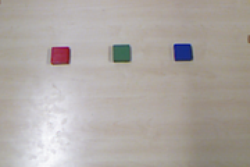
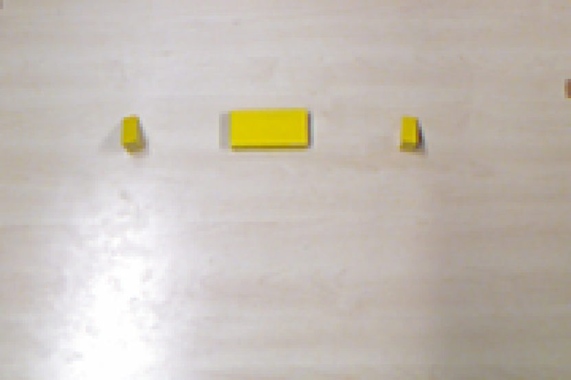
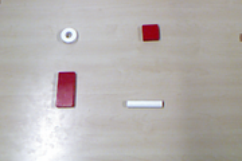
[b].196 [b].196 [b].196 [b].196 [b].196

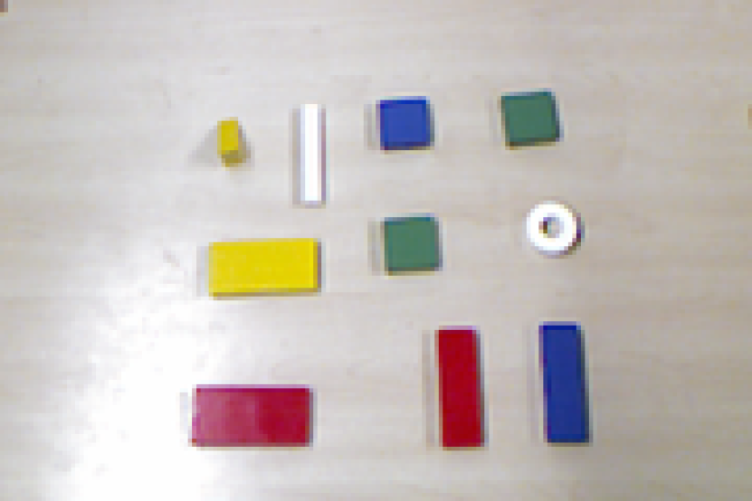
Figure 2: $\env_{1.1}$

Figure 3: $\env_{2.4}$

Figure 4: $\env_{3.5}$

Figure 5: $\env_{4.2}$

Figure 6: $\env_{5.1}$

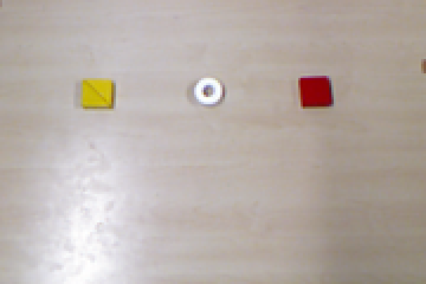
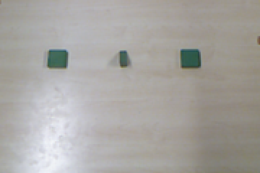
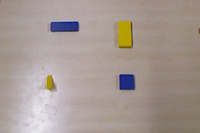
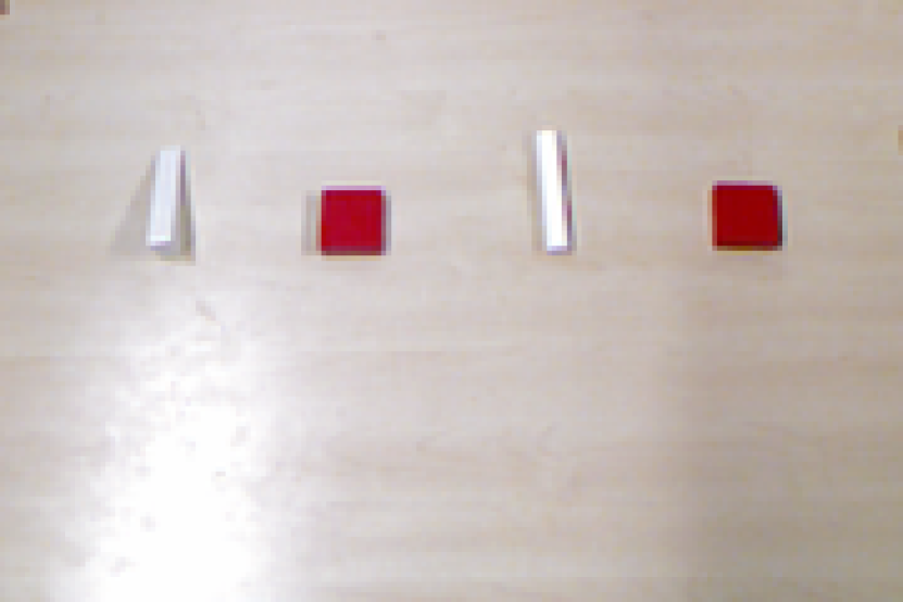
[b].196 [b].196 [b].196 [b].196 [b].196

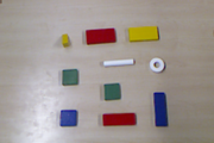
Figure 7: $\env_{1.4}$

Figure 8: $\env_{2.2}$

Figure 9: $\env_{3.3}$

Figure 10: $\env_{4.5}$

Figure 11: $\env_{5.2}$

Figure 12: The images depict 10 of the 22 environments used for training. Each column contains 2 samples from each category. The first category contains environments where three differently colored blocks are positioned side by side; the second category contains environments in which blocks of the same color have to be identified through their geometry of position. The third category contains blocks of 2 colors positioned in way that each block has a variery of correct descriptions which may be used to identify it. The fourth category contains environments in which a correct identification can sometimes only be achieved by learning an appropriate trade-off between the relevancy of positional and chromatic features. The fifth category only contains 2 environments in which the many objects are located in no particular order and without any pattern.

IV-B Training Data

To train and evaluate the model, we collected a data-set of object descriptions and one of object identifications.

IV-B1 Description Data

The data-set consists of 22 environments, which we denote as $\env_{[1\textnormal{-}4].[1\textnormal{-}5]}$ and $\env_{5.[1\textnormal{-}2]}$ and differ in the number of objects, their properties, and/or their disposition on the table (dtask_data). We partition these into 5 categories $\gamma_{i}=\{\env_{i.*}\}$ which broadly share some underlying theme or pattern, respectively containing 5, 5, 5, 5 and 2 environments. Multiple descriptions are provided for each object in each environment, ranging from overly-specific to ambiguous ones, for a total of 660 descriptions in the whole dataset.

IV-B2 Identification Data

Each description is interpreted by 10 users, resulting in 6600 identification data-points. The users are instructed, for each description, to select all objects which are plausible subjects of the description according to their interpretation. The corresponding target distribution is constructed such that the objects which have not been selected assume a low probability mass of 0.005, while the rest of the mass is uniformly distributed among all selected objects.

IV-C Performance Statistics

Given an environment $\env$, we define a partition of the dataset $D=D_{\env}\bigcup D_{\setminus\env}$, where $D_{\env}$ contains all data regarding environment $\env$, and $D_{\setminus\env}$ is its complement. Given a category $\gamma$, we further define a partition of the dataset $D=D_{\gamma}\bigcup D_{\setminus\gamma}$, where $D_{\gamma}=\bigcup_{\env\in\gamma}D_{\env}$, and $D_{\setminus\gamma}$ is the complement.

We perform cross-validation using both environment-induced partitions and category-induced partitions. Performing cross-validation on the category-induced partitions further ensures that the model evaluation does not suffer from overfitting, due to the shared high-level patterns which however don’t influence the identification task.

In the first evaluation, we iterate through all environments $\env$ and use $D_{\setminus\env}$ to train the model and $D_{\env}$ to evaluate it. We then repeat the process iterating through al categories $\gamma$, using $D_{\setminus\gamma}$ and $D_{\gamma}$ respectively for training and testing.

The results—which are summarized in cv—indicate that the model suffers the most in situations where chromatic features are undiscriminative and irrelevant. The lower-than-average performance on category $\gamma_{5}$ may be a consequence of the number of objects, which is at least double compared to all the other environments in the data-set.

TABLE I: Evaluation Statistics computed by cross-validation using environment-based splits and category-based splits. Column t_lklh contains the fraction of posterior identity mass $\pr(\obj\cond\desc)$ which is correctly assigned to the objects selected by the target distribution; this is approximatively $q\T p$, with $q$ and $p$ from loss. Column $\KL$ contains the average KL-divergence loss per identification task [nats].

	t_lklh	$\KL$		t_lklh	$\KL$		t_lklh	$\KL$
$\env_{1.1}$	95.2%	0.04	$\env_{3.1}$	92.0%	0.12	$\env_{5.1}$	82.0%	0.29
$\env_{1.2}$	95.0%	0.04	$\env_{3.2}$	91.5%	0.14	$\env_{5.2}$	78.4%	0.32
$\env_{1.3}$	93.5%	0.05	$\env_{3.3}$	90.3%	0.18
$\env_{1.4}$	94.9%	0.04	$\env_{3.4}$	88.9%	0.21	$\gamma_{1}$	94.9%	0.04
$\env_{1.5}$	96.0%	0.04	$\env_{3.5}$	89.8%	0.18	$\gamma_{2}$	85.5%	0.24
$\env_{2.1}$	76.4%	0.39	$\env_{4.1}$	92.7%	0.11	$\gamma_{3}$	90.3%	0.17
$\env_{2.2}$	88.4%	0.16	$\env_{4.2}$	92.4%	0.16	$\gamma_{4}$	91.5%	0.13
$\env_{2.3}$	76.5%	0.36	$\env_{4.3}$	91.6%	0.11	$\gamma_{5}$	80.5%	0.31
$\env_{2.4}$	93.5%	0.08	$\env_{4.4}$	88.9%	0.19
$\env_{2.5}$	89.2%	0.23	$\env_{4.5}$	92.0%	0.11	$\avg$	86.3%	0.22

IV-D Online Real-World Demonstration

We further illustrate the identification model in an integrated real-world demonstration in which a PR2 robot observes blocks arbitrarily disposed on a table and, upon receiving the description of one of the blocks, identifies and grasps it.

The domain of this integrated demonstration is similar to the one in the training data-set, but allows us to test performance in a wider range of environments which differ even more from the ones used for training. test illustrates a selection of results obtained during the execution of the integrated demonstrations.

The demonstration pipeline depicted in demo mainly consists of 4 components: an object extration module, the identification model presented in this work, a grasping heuristic valid for our blocks domain, and a trajectory optimization routine for grasping.

IV-D1 Object Extraction

We use the Object Recognition Kitchen (ORK) [1], a ROS package which specializes in plane extraction and (modeled) object recognition, but which also clusters all points which do not match any of the extracted plane.

We select all clusters in 3D space which appear above the table plane, project them onto the 2D image and compute their convex-hulls, which represent binary masks through which the previously mentioned image features can be computed for each object.

IV-D2 Grasping Heuristic

We heuristically determine the optimal grasping position for an object by finding the horizontal direction vector $d$ along which the projected object point-cloud $P$ assumes the minimal thickness:

$$\argmin_{d} \left[\max_{x\in P}d\T x-\min_{x\in P}d\T x\right]$$

s.t.

$$\|d\| =1,$$

$$d\T z =0,$$

where $z$ is a vertical vector in the world frame. Grasping position is set as the mean position of the point-cloud $P$.

IV-D3 Trajectory Optimization

We use k-order Markov motion optimization [10] to plan the motion for grasping the object. We define a cost function that consists of the gripper position and orientation during the grasp. We additionally ensure safe motions by including collision avoidance and joint limit limit constraints into the problem formulation.

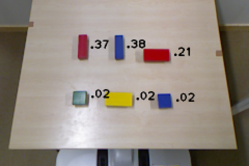
[b].246 [b].246 [b].246 [b].246

Figure 13: top

Figure 14: tall

Figure 15: red

Figure 16: right

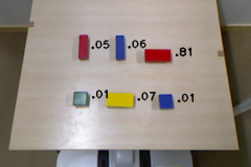
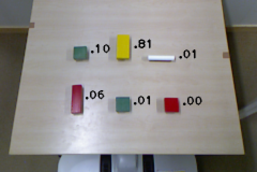
[b].246 [b].246 [b].246 [b].246

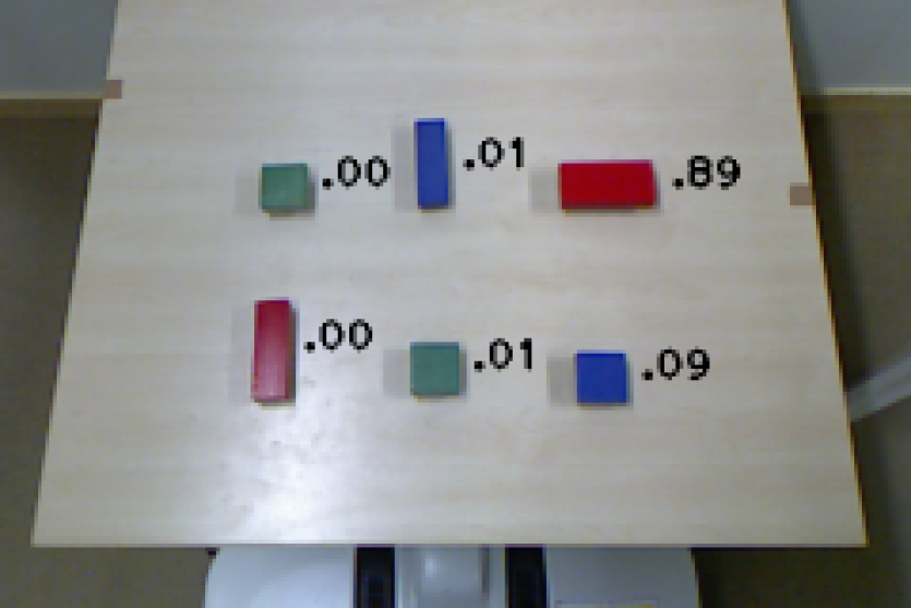
Figure 17: top wide

Figure 18: tall top

Figure 19: red thin

Figure 20: right wide

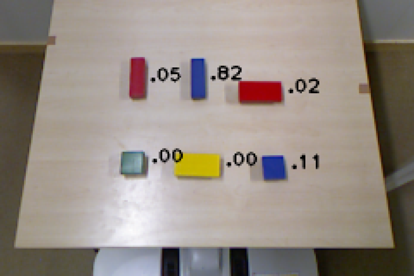
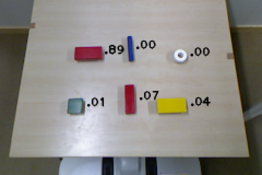
[b].246 [b].246 [b].246 [b].246

Figure 21: top blue

Figure 22: tall red

Figure 23: red wide

Figure 24: right bottom

Figure 25: Object identity posterior distributions for a selection of previously unseen environments. Each column represents the same environment where different descriptions are provided. The first row depicts the model output when provided with inherently ambiguous descriptions. In the second and third rows, the descriptions are extended, thus resolving the ambiguity in one way or another. Each environment is novel and demonstrates the model’s generalization properties in the sense that, while the same objects were used during training, these particular dispositions have never been seen before.

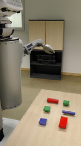
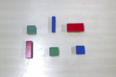
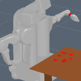
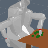
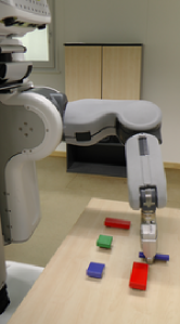
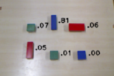
(A) at (0,0)[draw=black] ; [draw=black, right=4cm of A.north, anchor=north] (B) ; [draw=black, right=4cm of A.south, anchor=south] (C) ; [draw=black, right=4cm of C.south, anchor=south] (E) ; [above=1.33cm of E.north, anchor=south] (D) tall top ; [draw=black, right=4cm of E.south, anchor=south] (G) ; [draw=black, right=4cm of G.south, anchor=south] (H) ; [draw=black, left=4cm of H.north, anchor=north] (F) ; [line width=2pt] (A.east —- B.west) edge[-¿] (B.west); [line width=2pt] (A.east —- C.west) edge[-¿] (C.west); [line width=2pt] (C.north) edge[-¿] (B.south); [line width=2pt] (C.east) edge[-¿] (E.west); [line width=2pt] (E.east) edge[-¿] (G.west); [line width=2pt] (G.east) edge[-¿] (G.east -— H.west); [line width=2pt] (F.east) edge[-¿] (F.east -— H.west); [line width=2pt] (D.west) edge (B.east —- D.west); [line width=2pt] (D.east) edge[-¿] (D.east -— F.west); [line width=2pt] (F.south) edge[-¿] (G.north);

Figure 26: Object grasping demonstration on a PR2. The Object Recognition Kitchen ors package provides table-top plane extraction and object clusters (in red). Box models are fitted (in green) in order to find an adequate grasping direction, while our model computes the identity distribution upon receiving the description tall top. Finally, the robot proceeds to successfully grasp the correct object along an appropriate axis.

V CONCLUSIONS

In this work we propose and evaluate a discriminative model which is able to interpret object descriptions and decode the intended object identity. Quantitative and qualitative tests demonstrate positive identification capabilities, and an implementation on a PR2 robot demonstrates the usage in a real-world scenario in which unmodeled objects are being recognized by their description.

V-A Further Work

The work presented in this submisison is not meant to be conclusive, but rather represents a stepping stone towards more sophisticated methods to bridge the gap between perception and geometric and symbolic representations. We identify the following extensions and topics of interest for the further development.

While the focus of this work has been on the topic of object identification, the whole premise of successful human-robot communication requires a bidirectional exchange of information. An extension of direct interest consists in building on top of the discriminative identification model to obtain a generative description model which is able to produce sparse and minimal symbolic descriptions understandable by humans.

Another extension of immediate interest involves the usage of relational symbols. Their inclusion in the framework would greatly extend the space of existing descriptions in an environment, which produces two benefits: it increases the chance that an appropriate description exists for any given object—albeit this is true for any extension of the lexicon— and it potentially decreases the minimal complexity of a description required to describe an object.

The experiments presented in our work have considered a relatively simple lexicon, and simple object features extracted exclusively from image segments. Future effort should also focus on applying the model in more extensive domains where a bigger lexicon implies a wider range of possible descriptions, and in which more informative features (3D point-cloud features) may be required to successfully perform the identification task.

References

- [1] ORK: Object Recognition Kitchen.
- [2] A. Farhadi, I. Endres, D. Hoiem, and D. Forsyth. Describing objects by their attributes. In Computer Vision and Pattern Recognition, 2009. CVPR 2009. IEEE Conference on, pages 1778–1785, June 2009.
- [3] C. H. Lampert, H. Nickisch, and S. Harmeling. Learning to detect unseen object classes by betweenclass attribute transfer. In In CVPR, 2009.
- [4] G. Salvi, L. Montesano, A. Bernardino, and J. Santos-Victor. Language bootstrapping: Learning word meanings from perception-action association. IEEE Transactions on Systems, Man, and Cybernetics, Part B, 42(3):660–671, 2012.
- [5] B. Schauerte and R. Stiefelhagen. Look at this! learning to guide visual saliency in human-robot interaction. In Proceedings of the 27th International Conference on Intelligent Robots and Systems (IROS), Chicago, IL, USA, September 14-18 2014. IEEE/RSJ.
- [6] L. Steels. Constructing and sharing perceptual distinctions. In M. van Someren and G. Widmer, editors, Machine Learning: ECML-97, volume 1224 of Lecture Notes in Computer Science, pages 4–13. Springer Berlin Heidelberg, 1997.
- [7] L. Steels. The origins of syntax in visually grounded robotic agents. Artificial Intelligence, 103(1–2):133 – 156, 1998. Artificial Intelligence 40 years later.
- [8] L. Steels. Language games for autonomous robots. IEEE Intelligent Systems, 16(5):16–22, Sept. 2001.
- [9] S. Tellex, R. Knepper, A. Li, D. Rus, and N. Roy. Asking for help using inverse semantics. Proceedings of Robotics: Science and Systems, Berkeley, USA, 2014.
- [10] M. Toussaint. KOMO: Newton methods for k-order Markov Constrained Motion Problems. e-Print arXiv:1407.0414, 2014.