Robust Distributed Control Protocols for Large Vehicular Platoons with Prescribed Transient and Steady State Performance

Abstract

In this paper, we study the longitudinal control problem for a platoon of vehicles with unknown nonlinear dynamics under both the predecessor-following and the bidirectional control architectures. The proposed control protocols are fully distributed in the sense that each vehicle utilizes feedback from its relative position with respect to its preceding and following vehicles as well as its own velocity, which can all be easily obtained by onboard sensors. Moreover, no previous knowledge of model nonlinearities/disturbances is incorporated in the control design, enhancing in that way the robustness of the overall closed loop system against model imperfections. Additionally, certain designer-specified performance functions determine the transient and steady-state response, thus preventing connectivity breaks due to sensor limitations as well as inter-vehicular collisions. Finally, extensive simulation studies and a real-time experiment conducted with mobile robots clarify the proposed control protocols and verify their effectiveness.

I Introduction

During the last few decades, Automated Highway Systems (AHS) have drawn a notable amount of attention in the field of automatic control. Unlike human drivers, that are not able to react quickly and accurately enough to follow each other in close proximity at high speeds, the safety and capacity of highways (measured in vehicles/lanes/time) is significantly increased when vehicles operate autonomously forming large platoons at close spacing.

Guaranteed string stability [1] was first achieved via centralized control schemes [2, 3, 4], with all vehicles either communicating explicitly with each other or sending information to a central computer that determined the control protocol. To enhance the overall system’s autonomy and avoid delay problems due to wireless communication [5], decentralized schemes were developed, dealing either with the predecessor-following (PF) architecture [6, 7, 8], where each vehicle has access to its relative position with respect to its preceding vehicle, or the bidirectional (BD) architecture [9, 10, 11], where each vehicle measures its relative position with respect to its following vehicle as well. Furthermore, in a few works [5, 12] a combined predecessor and leader-following architecture was developed according to which each vehicle obtains additional information from the leading vehicle. Finally, [13, 14] addressed various architectures by examining different kinds of information flow topologies.

The majority of the works in the related literature either considers linear vehicle dynamic models and controllers [8, 15, 16] or adopt linearization techniques and Linear Quadratic optimal control [6, 13, 14, 9]. However, linearization may lead to unstable inner dynamics since the estimated linear models deviate in general from the real ones, away from the corresponding linearization points. In particular, a comparison of the aforementioned control architectures was carried out in [16], where it was stated that double integrator models with linear controllers under the predecessor-following architecture may lead to string instability. String instability conditions were also presented in [17]. Finally, in [18] a comparison of two common control policies was conducted; namely the constant time headway policy and the constant spacing policy, that are related to the inter-vehicular distances of the platoon. Particularly for the latter, it was also stated that feedback from the leading vehicle needs to be constantly broadcasted.

Another important issue associated with the decentralized control of large platoons of vehicles, concerns the fact that in many works the transient and steady state response of the closed loop system is affected severely by the control gains’ selection and the number of vehicles as stated in [10, 11, 16], limiting thus the controller’s capabilities. Furthermore, the majority of the results on the aforementioned decentralized architectures consider known (either partially of fully) dynamic models and parameters, which may lead to poor closed loop performance in the presence of parametric uncertainties and unknown external disturbances.

In this work, we propose decentralized control protocols for large platoons of vehicles with $2^{nd}$ order uncertain nonlinear dynamics, under both the predecessor-following and the bidirectional control architectures. The desired feasible formation is created arbitrarily fast and is maintained with arbitrary accuracy avoiding simultaneously any connectivity breaks (owing to limited sensor capabilities) and inter-vehicular collisions. The developed schemes exhibit the following significant characteristics. First, they are purely distributed in the sense that the control signal of each vehicle is calculated based solely: a) on local relative position information with respect to its preceding and following vehicles, as well as b) on its own velocity, both of which can be easily acquired by its on-board sensors. Furthermore, their complexity proves to be considerably low. Very few and simple calculations are required to output the control signals. Additionally, they do not require any previous knowledge of the vehicle’s dynamic model parameters and no estimation models are employed to acquire such knowledge. Moreover, contrary to the related works, the transient and steady state response is fully decoupled by: i) the number of vehicles composing the platoon, ii) the control gains selection and iii) the vehicle model uncertainties. In particular, the achieved performance as well as the collision avoidance and the connectivity maintenance are a priori and explicitly imposed by certain designer-specified performance functions, thus simplifying significantly the selection of the control gains. Tuning of the controller gains is only confined to achieving reasonable control effort.

II Problem Statement

We consider the longitudinal formation control problem of $N$ vehicles with $2^{nd}$ order nonlinear dynamics:

$$\dot{p}_{i} =v_{i}$$

$$m_{i}\dot{v}_{i} =f_{i}(v_{i})+u_{i}+w_{i}(t)\text{, }i=1,\ldots,N$$ (1)

where $p_{i}$ and $v_{i}$ denote the position and velocity of each vehicle respectively, $m_{i}$ is the mass, which is considered unknown, $f_{i}(v_{i})$ is an unknown continuous nonlinear function that models the aerodynamic friction (drag), $u_{i}$ is the control input and $w_{i}(t)$ is a bounded piecewise continuous function of time representing exogenous disturbances. The control objective is to design a distributed control protocol such that a rigid formation is established with prescribed transient and steady state performance, despite the presence of model uncertainties. By prescribed performance, we mean that the formation is achieved in a predefined transient period and is maintained arbitrarily accurate while avoiding connectivity breaks and collisions with neighboring vehicles. The geometry of the formation is represented by the desired gaps $\Delta_{i-1,i}$, $i=1,\ldots,N$ between consecutive vehicles, where $\Delta_{i-1,i}>0$ denotes the desired distance between the $(i-1)$-th and $i$-th vehicle. In general, all $\Delta_{i-1,i}$ are given as control specifications and are directly related to the platoon velocity as well as to the input constraints of the traction/bracking forces (for safety reasons). Moreover, the inter-vehicular distance $p_{i-1}(t)-p_{i}(t)$, $i=1,\dots,N$ should be kept greater than $\Delta_{\mathsf{col}}$ to avoid collisions and less than $\Delta_{\mathsf{con}}$ to maintain the network connectivity owing to the limited sensing capabilities of the vehicles (e.g., when employing range sensors to measure the distance between two successive vehicles). Furthermore, to ensure the feasibility of the desired formation, we assume that $\Delta_{\mathsf{col}}<\Delta_{i-1,i}<\Delta_{\mathsf{con}}$, $i=1,\ldots,N$. Additionally, the reference command of the formation is generated by a leading vehicle with position $p_{0}(t)$ and bounded velocity $v_{0}(t)$. Finally, to solve the aforementioned formation control problem, the following assumption is required.

Assumption A1. The initial state of the platoon does not violate the collision and connectivity constraints. That is $\Delta_{\mathsf{col}}<$ $p_{i-1}(0)-p_{i}(0)<\Delta_{\mathsf{con}},$ $i=1,\ldots,N$.

In this work, we consider two distributed control architectures: (a) the predecessor-following (PF) architecture, according to which the control action of each vehicle is based only on its preceding vehicle and (b) the bidirectional (BD) architecture, where the control action of each vehicle depends on the information from both its preceding and following vehicles. Hence, let us formulate the control variables $e_{p_{i}}(t)=p_{i-1}(t)-p_{i}(t)-\Delta_{i-1,i}$, $i=1,\ldots,N$. Equivalently, the neighborhood error vector $e_{p}\triangleq[e_{p_{1}},\ldots,e_{p_{N}}]^{T}$ may be expressed as follows:

$$e_{p}=Se_{p_{0}}$$ (2)

where $e_{p_{0}}\triangleq[e_{p_{0,1}},\ldots,e_{p_{0,N}}]^{T}=\bar{p}_{0}-p-\bar{\Delta}_{0}$ is the error with respect to the leading vehicle, $p\triangleq[p_{1},\ldots,p_{N}]^{T}\in\Re^{N},$ $\bar{p}_{0}\triangleq[p_{0},\ldots,p_{0}]^{T}\in\Re^{N}$, $\bar{\Delta}_{0}\triangleq[\Delta_{0,1},\Delta_{0,2},\ldots,\Delta_{0,N}]^{T}\in\Re^{N}$ with $\Delta_{0,i}=\sum_{j=1}^{i}\Delta_{j-1,j},$ $i=1,\ldots,N$ and $S\in\Re^{N\times N}=\left[s_{i,j}\right]$ where $s_{i,i}=1$, $s_{i+1,i}=-1$ and $s_{i,j}=0$ for all other elements, with $i,j=1,\dots,N$. Notice that $S$ has strictly positive singular values [3] and since all principal minors of $S$ are equal to $1,$ $S$ is also a nonsingular $\mathcal{M}$-matrix [20]. Finally, the following lemma regarding nonsingular $\mathcal{M}$-matrices will be employed to derive the main results of this paper.

Lemma 1.

[3] Consider a nonsingular $\mathcal{M}$-matrix $A\in\Re^{N\times N}$. There exists a diagonal positive definite matrix $P=$ $(\mathrm{diag}(A^{-1}\underline{\mathbf{1}}))^{-1}$ such that $PA+A^{T}P$ is positive definite.

III Main Results

In this work, prescribed performance will be adopted in order: i) to achieve predefined transient and steady state response for each neighborhood position error $e_{p_{i}}(t)$, $i=1,\ldots,N$ as well as ii) to avoid the violation of the collision and connectivity constraints as presented in Section II.

III-A Sufficient Conditions

Prescribed performance is achieved when the neighborhood position errors $e_{p_{i}}(t)$, $i=1,\ldots,N$ evolve strictly within predefined regions that are bounded by absolutely decaying functions of time, called performance functions [21, 19]. In this work, the mathematical expression of prescribed performance is formulated by the following inequalities:

$$-\underline{M}_{p_{i}}\rho_{p_{i}}\left(t\right)<e_{p_{i}}\left(t\right)<\overline{M}_{p_{i}}\rho_{p_{i}}\left(t\right)\text{, }\forall t\geq 0$$ (3)

for all $i=1,\ldots,N$, where:

$$\rho_{p_{i}}\left(t\right)=\left(1-\tfrac{\rho_{\infty}}{\max\{\underline{M}_{p_{i}},\overline{M}_{p_{i}}\}}\right)\exp\left(-lt\right)+\tfrac{\rho_{\infty}}{\max\{\underline{M}_{p_{i}},\overline{M}_{p_{i}}\}}$$ (4)

are designer-specified, smooth, bounded and decreasing functions of time with $l$, $\rho_{\infty}$ positive parameters incorporating the desired transient and steady state performance specifications respectively, and $\underline{M}_{p_{i}},$ $\overline{M}_{p_{i}}$, $i=1,\ldots,N$ positive parameters selected appropriately to satisfy the collision and connectivity constraints, as presented in the sequel. In particular, the decreasing rate of $\rho_{p_{i}}\left(t\right),$ $i=1,\ldots,N$, which is affected by the constant $l$, introduces a lower bound on the speed of convergence of $e_{p_{i}}(t),$ $i=1,\ldots,N$. Furthermore, depending on the accuracy of the measurement device, the constant $\rho_{\infty}$ can be set arbitrarily small $\rho_{\infty}\ll\underline{M}_{p_{i}},\overline{M}_{p_{i}}$, $i=1,\dots,N$, thus achieving practical convergence of $e_{p_{i}}(t)$, $i=1,\ldots,N$ to zero. Additionally, we select:

$$\underline{M}_{p_{i}}=\Delta_{i-1,i}-\Delta_{\mathsf{col}}\And\overline{M}_{p_{i}}=\Delta_{\mathsf{con}}-\Delta_{i-1,i}\text{, }i=1,\dots,N.$$ (5)

Apparently, since the desired formation is compatible with the collision and connectivity constraints (i.e., $\Delta_{\mathsf{col}}<\Delta_{i-1,i}<\Delta_{\mathsf{con}},$ $i=1,\dots,N$), (5) ensures that $\underline{M}_{p_{i}},$ $\overline{M}_{p_{i}}>0,$ $i=1,\dots,N$ and consequently under Assumption A1 (i.e., $\Delta_{\mathsf{col}}<$ $p_{i-1}(0)-p_{i}(0)<\Delta_{\mathsf{con}},$ $i=1,\ldots,N$) that:

$$-\underline{M}_{p_{i}}\rho_{p_{i}}\left(0\right)<e_{p_{i}}\left(0\right)<\overline{M}_{p_{i}}\rho_{p_{i}}\left(0\right)\text{, }i=1,\dots,N.$$ (6)

Hence, guaranteeing prescribed performance via (3) for all $t>0$ and employing the decreasing property of $\rho_{p_{i}}\left(t\right)$, $i=1,\dots,N,$ we obtain $-\underline{M}_{p_{i}}<e_{p_{i}}\left(t\right)<\overline{M}_{p_{i}},$ $\forall t\geq 0$ and consequently, owing to (5), $\Delta_{\mathsf{col}}<p_{i-1}(t)-p_{i}(t)<\Delta_{\mathsf{con}}$ for all $t\geq 0$ and $i=1,\ldots,N$, which ensures collision avoidance and connectivity maintenance for all $t\geq 0$. Therefore, imposing prescribed performance via (3) with appropriately selected performance functions $\rho_{p_{i}}\left(t\right)$, $i=1,\dots,N$ and positive constant parameters $\underline{M}_{p_{i}},\overline{M}_{p_{i}}$, $i=1,\dots,N$, as dictated in (4) and (5) respectively, proves sufficient to solve the robust formation control problem stated in Section II.

III-B Control Design

Kinematic Controller: Given the neighborhood position errors $e_{p_{i}}\left(t\right)=p_{i-1}(t)-p_{i}(t)-\Delta_{i-1,i}$, $i=1,\ldots,N$:

Step I-a. Select the corresponding functions $\rho_{p_{i}}\left(t\right)$ and positive parameters $\underline{M}_{p_{i}},$ $\overline{M}_{p_{i}}$, $i=1,\ldots,N$ following (4) and (5) respectively, in order to incorporate the desired transient and steady state performance specifications as well as the collision and connectivity constraints.

Step I-b. Define the normalized position errors as:

$$\xi_{p}(e_{p},t)\triangleq\begin{bmatrix}\xi_{p_{1}}(e_{p_{1}},t)\\ \vdots\\ \xi_{p_{N}}(e_{p_{N}},t)\end{bmatrix}\triangleq\begin{bmatrix}\frac{e_{p_{1}}}{\rho_{p_{1}}\left(t\right)}\\ \vdots\\ \frac{e_{p_{N}}}{\rho_{p_{N}}\left(t\right)}\end{bmatrix}\equiv(\rho_{p}\left(t\right))^{-1}e_{p}\text{,}$$ (7)

where $\rho_{p}\left(t\right)=\mathrm{diag}\left([\rho_{p_{i}}\left(t\right)]_{i=1,\ldots,N}\right)$ as well as the control signals:

$$r_{p}(\xi_{p}) =\mathrm{diag}\left(\left[\tfrac{\frac{1}{\underline{M}_{p_{i}}}+\frac{1}{\overline{M}_{p_{i}}}}{(1+\frac{\xi_{p_{i}}}{\underline{M}_{p_{i}}})(1-\frac{\xi_{p_{i}}}{\overline{M}_{p_{i}}})}\right]_{i=1,\dots,N}\right)$$ (8)

$$\varepsilon_{p}(\xi_{p}) =\left[\ln\left(\tfrac{1+\frac{\xi_{p_{1}}}{\underline{M}_{p_{1}}}}{1-\frac{\xi_{p_{1}}}{\overline{M}_{p_{1}}}}\right),\ldots,\ln\left(\tfrac{1+\frac{\xi_{p_{N}}}{\underline{M}_{p_{N}}}}{1-\frac{\xi_{p_{N}}}{\overline{M}_{p_{N}}}}\right)\right]^{T}\text{.}$$ (9)

Step I-c. Design the reference velocity vector for the predecessor-following and bidirectional control architectures as follows:

A. Predecessor-Following architecture:

$$v_{d}(\xi_{p},t) \triangleq\begin{bmatrix}v_{d_{1}}(\xi_{p_{1}},t)\\ \vdots\\ v_{d_{N-1}}(\xi_{p_{N-1}},t)\\ v_{d_{N}}(\xi_{p_{N}},t)\end{bmatrix}$$

$$=k_{p}(\rho_{p}\left(t\right))^{-1}r_{p}(\xi_{p})\varepsilon_{p}(\xi_{p})\text{,}$$ (10)

B. Bidirectional architecture:

$$v_{d}(\xi_{p},t) \triangleq\begin{bmatrix}v_{d_{1}}(\xi_{p_{1}},\xi_{p_{2}},t)\\ \vdots\\ v_{d_{N-1}}(\xi_{p_{N-1}},\xi_{p_{N}},t)\\ v_{d_{N}}(\xi_{p_{N}},t)\end{bmatrix}$$

$$=k_{p}S^{T}(\rho_{p}\left(t\right))^{-1}r_{p}(\xi_{p})\varepsilon_{p}(\xi_{p})$$ (11)

with $k_{p}>0$.

Dynamic Controller:

Step II-a. Define the velocity error vector $e_{v}\triangleq[e_{v_{1}},\ldots,e_{v_{N}}]^{T}=v-v_{d}(\xi_{p},t)$ with $v\triangleq[v_{1},\ldots,v_{N}]^{T}$ for both control architectures and select the corresponding velocity performance functions $\rho_{v_{i}}\left(t\right),$ $i=1,\ldots,N$ such that $\rho_{v_{i}}\left(0\right)>\left|e_{v_{i}}(0)\right|$, $i=1,\ldots,N$.

Step II-b. Similarly to the first step define the normalized velocity errors as:

$$\xi_{v}(e_{v},t)\triangleq\begin{bmatrix}\xi_{v_{1}}(e_{v_{1}},t)\\ \vdots\\ \xi_{v_{N}}(e_{v_{N}},t)\end{bmatrix}\triangleq\begin{bmatrix}\frac{e_{v_{1}}}{\rho_{v_{1}}\left(t\right)}\\ \vdots\\ \frac{e_{v_{N}}}{\rho_{v_{N}}\left(t\right)}\end{bmatrix}\equiv(\rho_{v}\left(t\right))^{-1}e_{v}\text{,}$$ (12)

where $\rho_{v}\left(t\right)=\mathrm{diag}\left([\rho_{v_{i}}\left(t\right)]_{i=1,\ldots,N}\right)$ as well as the control signals:

$$r_{v}(\xi_{v}) =\mathrm{diag}\left(\left[\tfrac{2}{(1+\xi_{v_{i}})(1-\xi_{v_{i}})}\right]_{i=1,\dots,N}\right)$$ (13)

$$\varepsilon_{v}(\xi_{v}) =\left[\ln\left(\tfrac{1+\xi_{v_{1}}}{1-\xi_{v_{1}}}\right),\ldots,\ln\left(\tfrac{1+\xi_{v_{N}}}{1-\xi_{v_{N}}}\right)\right]^{T}\text{.}$$ (14)

Step II-c. Design the distributed control protocol for both architectures as follows:

$$u(\xi_{v},t)\triangleq\begin{bmatrix}u_{1}(\xi_{v_{1}},t)\\ \vdots\\ u_{N}(\xi_{v_{N}},t)\end{bmatrix}=-k_{v}(\rho_{v}\left(t\right))^{-1}r_{v}(\xi_{v})\varepsilon_{v}(\xi_{v})$$ (15)

with $k_{v}>0$.

Remark 1.

(Control Philosophy) The prescribed performance control technique guarantees the prescribed transient and steady state performance specifications, that are encapsulated in (3), by enforcing the normalized position errors $\xi_{p_{i}}\left(t\right)$ and velocity errors $\xi_{v_{i}}\left(t\right)$, $i=1,\dots,N$ to remain strictly within the sets $\left(-\underline{M}_{p_{i}},\overline{M}_{p_{i}}\right)$ and $\left(-1,1\right)$ respectively for all $t\geq 0$. Notice that modulating $\xi_{p_{i}}\left(t\right)$ and $\xi_{v_{i}}\left(t\right)$ via the logarithmic functions $\ln\left(\tfrac{1+\frac{\star}{\underline{M}_{p_{i}}}}{1-\frac{\star}{\overline{M}_{p_{i}}}}\right)$ and $\ln\left(\tfrac{1+\star}{1-\star}\right)$ in the control signals (9), (14) and selecting $\underline{M}_{p_{i}}$, $\overline{M}_{p_{i}}$ according to (5) and $\rho_{v_{i}}\left(0\right)>\left|e_{v_{i}}(0)\right|$, the control signals $\varepsilon_{p}(\xi_{p})$ and $\varepsilon_{v}(\xi_{v})$ are initially well defined. Moreover, it is not difficult to verify that maintaining simply the boundedness of the modulated errors $\varepsilon_{p}(\xi_{p}\left(t\right))$ and $\varepsilon_{v}(\xi_{v}\left(t\right))$ for all $t\geq 0$ is equivalent to guaranteeing $\xi_{p_{i}}\left(t\right)\in\left(-\underline{M}_{p_{i}},\overline{M}_{p_{i}}\right)$ and $\xi_{v_{i}}\left(t\right)\in\left(-1,1\right)$ for all $t\geq 0$. Therefore, the problem at hand can be visualized as stabilizing the modulated errors $\varepsilon_{p}(\xi_{p}\left(t\right))$ and $\varepsilon_{v}(\xi_{v}\left(t\right))$, within the feasible regions defined via $\xi_{p_{i}}\in\left(-\underline{M}_{p_{i}},\overline{M}_{p_{i}}\right)$ and $\xi_{v_{i}}\in\left(-1,1\right)$, $i=1,\dots,N$ for all $t\geq 0$. A careful inspection of the proposed control scheme (10), (11) and (15) reveals that it actually operates similarly to barrier functions in constrained optimization, admitting high negative or positive values depending on whether $e_{p_{i}}\left(t\right)\rightarrow-\underline{M}_{p_{i}}\rho_{p_{i}}\left(t\right)$ and $e_{v_{i}}\left(t\right)\rightarrow\rho_{v_{i}}\left(t\right)$ or $e_{p_{i}}\left(t\right)\rightarrow\overline{M}_{p_{i}}\rho_{p_{i}}\left(t\right)$ and $e_{v_{i}}\left(t\right)\rightarrow-\rho_{v_{i}}\left(t\right)$, $i=1,\dots,N$ respectively; eventually preventing $e_{p_{i}}\left(t\right)$ and $e_{v_{i}}\left(t\right)$, $i=1,\dots,N$ from reaching the corresponding boundaries.

Remark 2.

(Selecting the Performance Functions) Regarding the construction of the performance functions, we stress that the desired performance specifications concerning the transient and steady state response as well as the collision and connectivity constraints are introduced in the proposed control schemes via $\rho_{p_{i}}\left(t\right)$ and $\underline{M}_{p_{i}}$, $\overline{M}_{p_{i}}$, $i=1,\dots,N$ respectively. In addition, the velocity performance functions $\rho_{v_{i}}\left(t\right)$ impose prescribed performance on the velocity errors $e_{v_{i}}=v_{i}-v_{d_{i}}$, $i=1,\dots,N$. In this respect, notice that $v_{d_{i}}$ act as reference signals for the corresponding velocities $v_{i}$, $i=1,\dots,N$. However, it should be stressed that although such performance specifications are not required (only the neighborhood position errors need to satisfy predefined transient and steady state performance specifications) their selection affects both the evolution of the position errors within the corresponding performance envelopes as well as the control input characteristics (magnitude and rate). Nevertheless, the only hard constraint attached to their definition is related to their initial values. Specifically, $\rho_{v_{i}}\left(0\right)$ should be chosen to satisfy $\rho_{v_{i}}\left(0\right)>\left|e_{v_{i}}(0)\right|$, $i=1,\ldots,N$.

III-C Stability Analysis

The main results of this work are summarized in the following theorem, where it is proven that the aforementioned distributed control protocols solve the robust formation problem with prescribed performance under collision and connectivity constraints for the considered platoon of vehicles.

Theorem 1.

Consider a platoon of $N$ vehicles with uncertain 2nd order nonlinear dynamics (1), that aims at establishing a formation described by the desired inter-vehicular gaps $\Delta_{i-1,i}$, $i=1,\ldots,N$, while satisfying the collision and connectivity constraints represented by $\Delta_{\mathsf{col}}$ and $\Delta_{\mathsf{con}}$ respectively with $\Delta_{\mathsf{col}}<\Delta_{i-1,i}<\Delta_{\mathsf{con}}$, $i=1,\ldots,N$. Under Assumption A1, the distributed control protocols (7)-(15), for the predecessor-following and bidirectional control architectures, guarantee: $-\underline{M}_{p_{i}}\rho_{p_{i}}\left(t\right)<e_{p_{i}}\left(t\right)<\overline{M}_{p_{i}}\rho_{p_{i}}\left(t\right)\text{, }$ for all $t\geq 0$ and $i=1,\ldots,N$, as well as the boundedness of all closed loop signals.

Proof: The proof of Theorem 1 proceeds in three phases. First, we show that $\xi_{p_{i}}\left(t\right)$ and $\xi_{v_{i}}\left(t\right)$ remain within $\left(-\underline{M}_{p_{i}},\overline{M}_{p_{i}}\right)$ and $\left(-1,1\right)$ respectively, for a specific time interval $\left[0,\tau_{\max}\right)$ (i.e., existence of a maximal solution). Next, we prove that the proposed control scheme retains $\xi_{p_{i}}\left(t\right)$ and $\xi_{v_{i}}\left(t\right)$ strictly in compact subsets of $\left(-\underline{M}_{p_{i}},\overline{M}_{p_{i}}\right)$ and $\left(-1,1\right)$ for all $t\in\left[0,\tau_{\max}\right)$, which by contradiction leads to $\tau_{\max}=\infty$ (i.e., forward completeness) in the last phase, thus completing the proof. It should be also noticed that the proof is provided only for the predecessor-following architecture since the proof for the bidirectional case follows identical steps.

In particular, by differentiating (7) and (12), we obtain:

$$\dot{\xi}_{p} =(\rho_{p}\left(t\right))^{-1}(\dot{e}_{p}-\dot{\rho}_{p}\left(t\right)\xi_{p})$$ (16)

$$\dot{\xi}_{v} =(\rho_{v}\left(t\right))^{-1}(\dot{e}_{v}-\dot{\rho}_{v}\left(t\right)\xi_{v})$$ (17)

Employing (1), (2) as well as the fact that $v_{i}\equiv v_{d_{i}}+\rho_{v_{i}}\left(t\right)\xi_{v_{i}}$ and substituting (10), (15) in (16) and (17), we arrive at:

$$\dot{\xi}_{p} =h_{p_{A}}(t,\xi)$$

$$=-k_{p}(\rho_{p}\left(t\right))^{-1}S(\rho_{p}\left(t\right))^{-1}r_{p}(\xi_{p})\varepsilon_{p}(\xi_{p})$$

$$\text{ \ \ }-(\rho_{p}\left(t\right))^{-1}(\dot{\rho}_{p}\left(t\right)\xi_{p}+S(\rho_{v}\left(t\right)\xi_{v}-\dot{\overline{p}}_{0}(t)))$$ (18)

$$\dot{\xi}_{v} =h_{v_{A}}(t,\xi)$$

$$=-k_{v}(\rho_{v}\left(t\right))^{-1}M^{-1}\varepsilon_{v}(\xi_{v})-(\rho_{v}\left(t\right))^{-1}(\dot{\rho}_{v}\left(t\right)\xi_{v}$$

$$\text{ \ \ }-M^{-1}(f(v_{d}+\rho_{v}\left(t\right)\xi_{v})+w(t))+\dot{v}_{d})$$ (19)

where $M=\mathrm{diag}\left(\left[m_{i}\right]_{i=1,\ldots,N}\right)$ and $f(v_{d}+\rho_{v}\left(t\right)\xi_{v})=\left[f_{1}(v_{d_{1}}+\rho_{v_{1}}\left(t\right)\xi_{v_{1}}),\cdots,f_{N}(v_{d_{N}}+\rho_{v_{N}}\left(t\right)\xi_{v_{N}}\right]^{T}$ with $m_{i}$, $f_{i}(\cdot)$, $i=1,\ldots,N$ denoting the unknown masses and nonlinearities of the vehicle model (1) respectively. Thus, the closed loop dynamical system of $\xi(t)=\left[\xi_{p}^{T}(t),\xi_{v}^{T}(t)\right]^{T}$ may be written in compact form as:

$$\dot{\xi}=h_{A}(t,\xi)\triangleq\begin{bmatrix}h_{p_{A}}(t,\xi)\\ h_{v_{A}}(t,\xi)\end{bmatrix}.$$ (20)

Let us also define the open set $\Omega_{\xi}=\Omega_{\xi_{p}}\times\Omega_{\xi_{v}}\subset\Re^{2N}$ with:

$$\Omega_{\xi_{p}} =(-\underline{M}_{p_{1}},\overline{M}_{p_{1}})\times\cdots\times(-\underline{M}_{p_{N}},\overline{M}_{p_{N}})$$

$$\Omega_{\xi_{v}} =\underbrace{(-1,1)\times\cdots\times(-1,1)}_{N\text{-times}}\text{.}$$ (21)

Phase I. Selecting the parameters $\underline{M}_{p_{i}},$ $\overline{M}_{p_{i}},$ $i=1,\ldots,N$ according to (5), we guarantee that the set $\Omega_{\xi}$ is nonempty and open. Moreover, owing to Assumption A1, $\xi_{p}(0)\in\Omega_{\xi_{p}}$, as shown in (6). Furthermore, selecting $\rho_{v_{i}}\left(0\right)>\left|e_{v_{i}}(0)\right|,$ $i=1,\ldots,N$ ensures that $\xi_{v}(0)\in\Omega_{\xi_{v}}$ as well. Thus, we conclude that $\xi(0)\in\Omega_{\xi}$. Additionally, $h_{A}$ is continuous on $t$ and locally Lipschitz on $\xi$ over the set $\Omega_{\xi}$. Therefore, the hypotheses of Theorem 54 in [22] (p.p. 476) hold and the existence of a maximal solution $\xi(t)$ of (20) for a time interval $[0,\tau_{\max})$ such that $\xi(t)\in\Omega_{\xi},$ $\forall t\in[0,\tau_{\max})$ is guaranteed.

Phase II-Kinematics. We have proven in Phase I that $\xi(t)\in\Omega_{\xi},$ $\forall t\in[0,\tau_{\max})$ and more specifically that:

$$\left.\begin{array}[c]{l}\xi_{p_{i}}\left(t\right)=\frac{e_{p_{i}}(t)}{\rho_{p_{i}}(t)}\in(-\underline{M}_{p_{i}},\text{ }\overline{M}_{p_{i}})\\ \xi_{v_{i}}\left(t\right)=\frac{e_{v_{i}}(t)}{\rho_{v_{i}}(t)}\in(-1,1)\end{array}\right\}\text{ }i=1,\dots,N$$ (22)

for all $t\in[0,\tau_{\max})$, from which we obtain that $e_{p_{i}}(t)$ and $e_{v_{i}}(t)$ are absolutely bounded by $\max\{\underline{M}_{p_{i}},$ $\overline{M}_{p_{i}}\}\rho_{p_{i}}(t)$ and $\rho_{v_{i}}(t)$ respectively for $i=1,\dots,N.$ Furthermore, owing to (22), the error vector $\varepsilon_{p}(t)$, as defined in (9), is well defined for all $t\in[0,\tau_{\max})$. Therefore, consider the positive definite and radially unbounded function $V_{p_{A}}=\frac{1}{2}\varepsilon_{p}^{T}P\varepsilon_{p}$, where $P\triangleq($diag$(S^{-1}\underline{\mathbf{1}}))^{-1}$ is a diagonal positive definite matrix satisfying $PS+S^{T}P>0$, as dictated by Lemma 1. Differentiating $V_{p_{A}}$ with respect to time, substituting (8), (18) and exploiting: i) the diagonality of the matrices $P$, $r_{p}(\xi_{p})$, $\rho_{p}\left(t\right)$, ii) the positive definiteness of $Q\triangleq PS+S^{T}P$ as well as iii) the boundedness of $\dot{\rho}_{p}\left(t\right)$, $\rho_{v}\left(t\right)$ and $\dot{\overline{p}}_{0}(t)$, we get:

$$\dot{V}_{p_{A}} \leq-k_{p}\lambda_{\min}(Q)\left\|\varepsilon_{p}^{T}r_{p}(\xi_{p})(\rho_{p}\left(t\right))^{-1}\right\|^{2}$$

$$+\left\|\varepsilon_{p}^{T}r_{p}(\xi_{p})(\rho_{p}\left(t\right))^{-1}\right\|\bar{F}_{p}$$

where $F_{p}$ is a positive constant independent of $\tau_{\max}$, satisfying:

$$\left\|P(\dot{\rho}_{p}\left(t\right)\xi_{p}+S(\rho_{v}\left(t\right)\xi_{v}-\dot{\overline{p}}_{0}(t)))\right\|\leq\bar{F}_{p}$$ (23)

for all $(\xi,t)\in\Omega_{\xi}\times\Re_{+}$. Therefore, we conclude that $\dot{V}_{p_{A}}$ is negative when $\left\|\varepsilon_{p}^{T}r_{p}(\xi_{p})(\rho_{p}\left(t\right))^{-1}\right\|>\frac{\bar{F}_{p}}{k_{p}\lambda_{\min}(Q)}$, from which, owing to the positive definiteness and diagonality of $r_{p}(\xi_{p})(\rho_{p}\left(t\right))^{-1}$ as well as employing (8) and (4), it can be easily verified that:

$$\left\|\varepsilon_{p}(t)\right\|\leq\bar{\varepsilon}_{p}:=\tfrac{\lambda_{\max}(P)}{\lambda_{\min}(P)}\max\left\{\left\|\varepsilon_{p}(0)\right\|,\tfrac{\bar{F}_{p}\max\left\{\tfrac{\underline{M}_{p_{i}}\overline{\text{ }M}_{p_{i}}}{\underline{M}_{p_{i}}+\overline{\text{ }M}_{p_{i}}}\right\}}{k_{p}\lambda_{\min}(Q)}\right\}$$ (24)

for all $t\in[0,\tau_{\max})$. Furthermore, from (9), taking the inverse logarithm, we obtain:

$${\small-}\underline{M}_{p_{i}}{\small<-}\tfrac{\exp\left(\bar{\varepsilon}_{p}\right)-1}{\exp\left(\bar{\varepsilon}_{p}\right)+\frac{\underline{M}_{p_{i}}}{\overline{M}_{p_{i}}}}\underline{M}_{p_{i}}{\small=}\underline{\xi}_{p_{i}}{\small\leq\xi}_{p_{i}}{\small(t)}\\ {\small\leq\bar{\xi}}_{p_{i}}{\small=}\tfrac{\exp\left(\bar{\varepsilon}_{p}\right)-1}{\exp\left(\bar{\varepsilon}_{p}\right)+\frac{\overline{M}_{p_{i}}}{\underline{M}_{p_{i}}}}\overline{M}_{p_{i}}{\small<}\overline{M}_{p_{i}}$$ (25)

for all $t\in[0,\tau_{\max})$ and $i=1,\dots,N$. Thus, the reference velocity vector $v_{d}(\xi_{p},t),$ as designed in (10), remains bounded for all $t\in[0,\tau_{\max})$. Moreover, invoking $v_{i}\equiv v_{d_{i}}+\rho_{v_{i}}\left(t\right)\xi_{v_{i}}$ we also conclude the boundedness of the velocities $v_{i}(t),$ $i=1,\dots,N$ for all $t\in[0,\tau_{\max})$. Finally, differentiating $v_{d}(\xi_{p},t)$ with respect to time, substituting (18) and utilizing (25), it is straightforward to deduce the boundedness of $\dot{v}_{d}$ for all $t\in[0,\tau_{\max})$ as well.

Phase II-Dynamics. Owing to (22), the error vector $\varepsilon_{v}(t)$ (see (14)) is well defined for all $t\in[0,\tau_{\max})$. Therefore, consider the positive definite and radially unbounded function $V_{v_{A}}=\frac{1}{2}\varepsilon_{v}^{T}M\varepsilon_{v}$ where $M=\mathrm{diag}\left(\left[m_{i}\right]_{i=1,\ldots,N}\right)$ with $m_{i}$, $i=1,\dots,N$ denoting the unknown mass of the vehicle model (1). Following the same line of proof with $V_{p_{A}}$ in Phase II-Kinematics, we conclude that:

$$\left\|\varepsilon_{v}(t)\right\|\leq\bar{\varepsilon}_{v}:=\tfrac{\max\{m_{i}\}}{\min\{m_{i}\}}\max\left\{\left\|\varepsilon_{v}(0)\right\|,\tfrac{\bar{F}_{v}}{2k_{v}}\right\}$$ (26)

for all $t\in[0,\tau_{\max})$, where $\bar{F}_{v}$ is a positive constant satisfying:

$$\left\|(M\dot{\rho}_{v}\left(t\right)\xi_{v}-(f(v_{d}+\rho_{v}\left(t\right)\xi_{v})+w(t))+\dot{v}_{d})\right\|\leq\bar{F}_{v}$$ (27)

owing to: i) the boundedness of $v_{d}$ and $\dot{v}_{d}$ that was proven previously, ii) the continuity of function $f_{i}(\cdot)$ and iii) the boundedness of $\dot{\rho}_{v}\left(t\right)$, $\rho_{v}\left(t\right)$ as well as of the disturbance term $w(t)$. Furthermore, from (14), taking the inverse logarithmic function, we obtain:

$${\small-}1{\small<-}\tfrac{\exp\left(\bar{\varepsilon}_{v}\right)-1}{\exp\left(\bar{\varepsilon}_{v}\right)+1}{\small=}\underline{\xi}_{v_{i}}{\small\leq\xi}_{v_{i}}{\small(t)\leq\bar{\xi}}_{v_{i}}{\small=}\tfrac{\exp\left(\bar{\varepsilon}_{v}\right)-1}{\exp\left(\bar{\varepsilon}_{v}\right)+1}{\small<1}$$ (28)

for all $t\in[0,\tau_{\max})$ and $i=1,\dots,N$, which also leads to the boundedness of the distributed control protocol (15).

Phase III. Up to this point, what remains to be shown is that $\tau_{\max}$ can be extended to $\infty$. In this direction, notice by (25) and (28) that $\xi(t)\in\Omega_{\xi}^{{}^{\prime}}\triangleq\Omega_{\xi_{p}}^{{}^{\prime}}\times\Omega_{\xi_{v}}^{{}^{\prime}}$, $\forall t\in[0,\tau_{\max})$, where $\Omega_{\xi_{p}}^{{}^{\prime}}\triangleq\left[\underline{\xi}_{p_{1}},{\small\bar{\xi}}_{p_{1}}\right]\times\cdots\times\left[\underline{\xi}_{p_{N}},{\small\bar{\xi}}_{p_{N}}\right]$ and $\Omega_{\xi_{v}}^{{}^{\prime}}\triangleq\left[\underline{\xi}_{v_{1}},{\small\bar{\xi}}_{v_{1}}\right]\times\cdots\times\left[\underline{\xi}_{v_{N}},{\small\bar{\xi}}_{v_{N}}\right]$ are nonempty and compact subsets of $\Omega_{\xi_{p}}$ and $\Omega_{\xi_{v}}$ respectively. Hence, assuming $\tau_{\max}<\infty$ and since $\Omega_{\xi}^{{}^{\prime}}\subset\Omega_{\xi}$, Proposition C.3.6 in [22] (p.p. 481) dictates the existence of a time instant $t^{{}^{\prime}}\in[0,\tau_{\max})$ such that $\xi(t^{{}^{\prime}})\notin\Omega_{\xi}^{{}^{\prime}}$, which is a clear contradiction. Therefore, $\tau_{\max}$ is extended to $\infty$. Thus, all closed loop signals remain bounded and moreover $\xi(t)\in\Omega_{\xi}^{{}^{\prime}}\subset\Omega_{\xi}$, $\forall t\geq 0$. Finally, multiplying (25) by $\rho_{p_{i}}(t)$, $i=1,\dots,N$, we also conclude that:

$$-\underline{M}_{p_{i}}\rho_{p_{i}}\left(t\right)<e_{p_{i}}\left(t\right)<\overline{M}_{p_{i}}\rho_{p_{i}}\left(t\right)\text{, }\forall t\geq 0$$ (29)

for all $i=1,\dots,N$ and consequently the solution of the robust formation control problem with prescribed performance under collision and connectivity constraints for the considered platoon of vehicles. $\blacksquare$

Remark 3.

From the aforementioned proof it can be deduced that the proposed control schemes achieve their goals without resorting to the need of rendering the ultimate bounds $\bar{\varepsilon}_{p}$, $\bar{\varepsilon}_{v}$ of the modulated position and velocity errors $\varepsilon_{p}\left(\xi_{p}\left(t\right)\right)$, $\varepsilon_{v}\left(\xi_{v}\left(t\right)\right)$ arbitrarily small by adopting extreme values of the control gains $k_{p}$ and $k_{v}$ (see (24) and (26)). More specifically, notice that (25) and (28) hold no matter how large the finite bounds $\bar{\varepsilon}_{p}$, $\bar{\varepsilon}_{v}$ are. In the same spirit, large uncertainties involved in the vehicle nonlinear model (1) can be compensated, as they affect only the size of $\bar{\varepsilon}_{v}$ through $\bar{F}_{v}$ (see (27)), but leave unaltered the achieved stability properties. Hence, the actual performance given in (29), which is solely determined by the designer-specified performance functions $\rho_{p_{i}}\left(t\right)$ and the parameters $-\underline{M}_{p_{i}}$, $\overline{M}_{p_{i}}$, $i=1,\dots,N$, becomes isolated against model uncertainties, thus extending greatly the robustness of the proposed control schemes.

Figure 1: The position errors $e_{p_{i}}(t)$ (PF).

Figure 2: The required control input signals (PF).

Remark 4.

(Selecting the Control Gains) It should be noted that the selection of the control gains affects both the quality of evolution of the neighborhood errors $e_{p_{i}}\left(t\right)$, $i=1,\dots,N$ inside the corresponding performance envelopes as well as the control input characteristics (e.g., decreasing the gain values leads to increased oscillatory behaviour within the prescribed performance envelope described by (29), which is improved when adopting higher values, enlarging, however, the control effort both in magnitude and rate). Additionally, fine tuning might be needed in real-time scenarios, to retain the required control input signals within the feasible range that can be implemented by the actuators. Similarly, the control input constraints impose an upper bound on the required speed of convergence of $\rho_{p_{i}}\left(t\right)$, $i=1,\dots,N$, as obtained by the exponentials $\exp\left(-lt\right)$. Hence, the selection of the control gains $k_{p}$ and $k_{v}$ can have positive influence on the overall closed loop system response. More specifically, notice that (23)-(28) provide bounds on $\varepsilon_{p}$ and $\varepsilon_{v}$ that depend on the constants $\overline{F}_{p}$ and $\overline{F}_{v}$. Therefore, invoking (10),(11) and (15) we can select the control gains $k_{p}$ and $k_{v}$ such that $v_{d}$ and $u$ are retained within certain bounds. Nevertheless, the constants $\overline{F}_{p}$ and $\overline{F}_{v}$ involve the parameters of the model, the external disturbances, the velocity/acceleration of the leader and the desired performance specifications. Thus, an upper bound of the dynamic parameters of the system as well as of the exogenous disturbances must be given in order to extract any relationships between the achieved performance and the input constraints. Finally, in the same direction, the selection of the velocity performance functions $\rho_{v_{i}}\left(t\right)$, $i,\dots,N$ affects both the evolution of the position errors within the corresponding performance envelopes as well as the control input characteristics.

Remark 5.

(String Stability) Note that the proposed algorithm guarantees string stability for the equilibrium point $e_{p_{i}}=0,i=1,\dots,N$, in the sense of [1] (see Def. 1). In particular, for any $\epsilon>0$, we can choose $\delta=\max_{i}\{\max\{\underline{M}_{p_{i}},\overline{M}_{p_{i}}\}\}=\epsilon$, $i=1,\dots,N$. Then, from the aforementioned analysis it can be deduced that $\max_{i}\lvert e_{p_{i}}(0)\rvert<\delta$ implies $\max_{i}\{\sup_{t\geq 0}\lvert e_{p_{i}}(t)\rvert\}<\epsilon$, $i=1,\dots,N$.

IV Simulation Results

IV-A Generic Evaluation

To demonstrate the efficiency of the proposed distributed control protocols, we considered a platoon of $N=10$ vehicles obeying (1) with $f_{i}\left(v_{i}\right)=-50v_{i}-25\left|v_{i}\right|v_{i}$, $w_{i}\left(t\right)=A_{i}sin(\omega_{i}t+\phi_{i})$ and $m_{i}$, $A_{i}$, $\omega_{i}$, $\phi_{i}$ randomly selected within $\left[500,1500\right]$ kg, $[1.0,\,1.5]$ kNt, $[2\pi,\,4\pi]$ rad/s and $[0,\,2\pi]$ rad respectively for $i=1,\ldots,10$. Although the size of the aforementioned intervals affects directly the magnitude of the control effort $u$, which however can be regulated by tuning appropriately the gains $k_{p}$ and $k_{v}$, as mentioned in Remark 4, in view of the theoretical analysis, the uncertainty of the aforementioned parameters does not affect the performance of the proposed schemes. Furthermore, the leading vehicle adopts the following continuous velocity profile:

$$v_{0}\left(t\right)=\left\{\begin{array}[c]{lr}\frac{75t^{2}-t^{3}}{2500},&t\in\left[0,50\right]\\ 25,&t\in\left[50,70\right]\\ 0.02t^{3}-4.5t^{2}+336t-8305,&t\in\left[70,80\right]\\ 15,&t\in\left[80,90\right]\\ 17.5-2.5\cos\left(\frac{t-90}{2}\right),&t\in\left[90,120\right]\end{array}\right.\$$

whereas the desired distance between consecutive vehicles is equally set at $\Delta_{i-1,i}=\Delta^{\star}=4$ m, $i=1,\ldots,10$ with the collision and connectivity constraints given by $\Delta_{\mathsf{col}}=0.05\Delta^{\star}$ and $\Delta_{\mathsf{con}}=1.95\Delta^{\star}$ respectively. Notice that the aforementioned formation problem under the collision/connectivity constraints is feasible since $\Delta_{\mathsf{col}}<\Delta_{i-1,i}<\Delta_{\mathsf{con}}$, $i=1,\ldots,10$. Moreover, we require steady state errors of no more than $0.05$ m and minimum speed of convergence as obtained by the exponential $\exp\left(-0.1t\right)$. Thus, according to (4) and (5), we selected the parameters $\underline{M}_{p_{i}}=\overline{M}_{p_{i}}=0.95\Delta^{\star}$ and the functions $\rho_{p_{i}}(t)=(1-\frac{0.05}{0.95\Delta^{\star}})\exp\left(-0.1t\right)+\frac{0.05}{0.95\Delta^{\star}}$, $i=1,\ldots,10$ in order to achieve the desired transient and steady state performance specifications as well as to comply with the collision and connectivity constraints. Moreover, we chose $\rho_{v_{i}}(t)=2\left|e_{v_{i}}(0)\right|\exp\left(-0.1t\right)+0.1$ in order to satisfy $\rho_{v_{i}}\left(0\right)>\left|e_{v_{i}}\left(0\right)\right|$, $i=1,\ldots,10$. Finally, in view of the desired motion profile of the leader as well as the masses of the vehicles, we chose the control gains as $k_{p}=0.1,$ $k_{v}=100$ for the predecessor-following architecture and $k_{p}=10,$ $k_{v}=1000$ for the bidirectional architecture, to obtain control inputs that satisfy $\left|u_{i}\right|\leq 30$ kNt, $i=1,\dots,10$.

Figure 3: The position errors $e_{p_{i}}(t)$ (BD).

Figure 4: The required control input signals (BD).

The simulation results are illustrated in Figs. 2,2 and 4,4 for the predecessor-following (PF) and the bidirectional (BD) control architectures respectively. More specifically, the evolution of the neighborhood position errors $e_{p_{i}}(t)$, $i=1,\ldots,10$ along with the corresponding performance functions are depicted in Figs. 2 and 4, while the required control inputs are illustrated in Figs. 2 and 4. As it was predicted by the theoretical analysis, the formation control problem with prescribed transient and steady state performance is solved with bounded closed loop signals for both control architectures, despite the presence of external disturbances as well as the lack of knowledge of the vehicle dynamic model.

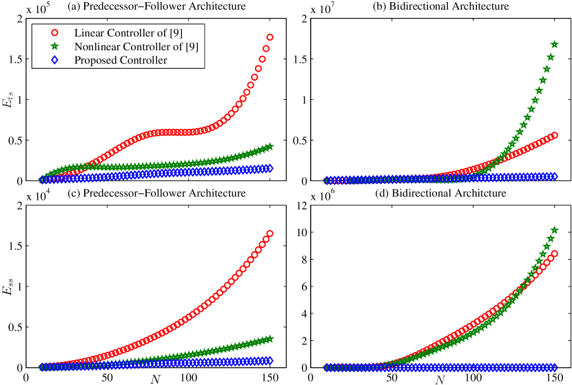
Figure 5: The error metrics $E_{ts}$ and $E_{ss}$ for the PF and BD architectures, as the number of vehicles $N$ increases.

IV-B Comparative Studies

To investigate further the performance of the proposed methodology, a comparative simulation study was carried out, on the basis of the aforementioned nonlinear model, among the proposed control schemes and the linear as well as nonlinear control protocols presented in [9]. For comparison purposes, we adopted the following metrics of performance:

$$E_{ts} =\frac{1}{N}\int_{0}^{t_{s}}\sum_{i=1}^{N}\{(e_{p_{0,i}}(t))^{2}+(\dot{e}_{p_{0,i}}(t))^{2}\}dt$$ (30)

$$E_{ss} =\frac{1}{N}\int_{t_{s}}^{T}\sum_{i=1}^{N}\{(e_{p_{0,i}}(t))^{2}+(\dot{e}_{p_{0,i}}(t))^{2}\}dt$$ (31)

for the transient and the steady state respectively, where $e_{p_{0,i}}(t)$, $i=1,\ldots,N$ denote the distance errors with respect to the leader, $t_{s}$ denotes the transient period and $T$ is the overall simulation time. In particular, we study through extensive numerical simulations how the metrics $E_{ts}$ and $E_{ss}$ scale with the number of agents $N\in\left[10,150\right]$ for $T=120$. It should be noticed that the methods proposed in [9] considered a double integrator model and therefore a feedback linearization technique was adopted in the control scheme initially. However, to simulate a realistic scenario, the model parameters adopted in the feedback linearization technique deviated up to $15\%$ from their actual values. Additionally, the corresponding control gains were selected through a tedious trial-and-error process to yield satisfactory performance for $N=10$. Regarding the proposed control schemes, the parameters were chosen as in Section IV-A, except for the steady state error bound and the minimum convergence speed of the performance functions $\rho_{p_{i}}\left(t\right),\rho_{v_{i}}\left(t\right)$. In particular, $\rho_{\infty}$ was calculated as $\rho_{\infty}=\frac{0.5\sigma_{\min}\left(S\right)}{\sqrt{N}}$, and the minimum speed of convergence was obtained by the exponential $\exp\left(-2t\right)$. Finally, the desired velocity profile of the leader and the desired inter-vehicular distances were set as in Section IV-A.

Figure 6: The position errors $e_{p_{i}}(t),i=1,\dots,4$.

Figure 7: The distance between successive vehicles.

Figure 8: The required control input signals.

The results of the comparative simulation study are given in Figs. 5a-5d. More specifically, Figs. 5a and 5b illustrate the evolution of $E_{ts}$ for the predecessor-following and the bidirectional control architecture respectively. Similarly, the evolution of $E_{ss}$ is given in Figs. 5c and 5d. Notice that the proposed control protocols render the metrics $E_{ts}$ and $E_{ss}$ almost invariant to the number of vehicles $N$. On the contrary, the performance of the linear and nonlinear control methodologies proposed in [9] deteriorated in both control architectures as the number of vehicles increased, proving thus the superiority of the proposed control protocols.

V Experimental Results

To verify the performance of the proposed scheme, an experimental procedure was carried out for the case of the predecessor-following architecture. The experiment took place along a $10$ m long hallway and lasted approximately $18$ seconds. Five mobile robots were employed. Particularly, a Pioneer2AT was assigned as the leading vehicle whereas two KUKA youBot platforms and two Pioneer2DX mobile robots consisted the following vehicles. To acquire the inter-vehicular distance measurements, infrared proximity sensors operating from $5$ to $65$ cm were utilized. The control scheme was designed at the kinematic level, i.e. the control inputs were the desired velocities (10) since the embedded motor controller of the vehicles was responsible for implementing the actual wheel torque commands that achieved the desired velocities.

The leader adopted a constant velocity model given by $p_{0}(t)=0.3t$ m and $v_{0}\left(t\right)=0.3$ m/s. The desired inter-vehicular distances were set at $\Delta_{i-1,i}=\Delta^{\star}=0.2$ m, $i=1,\ldots,4$, whereas the collision and connectivity constraints were given by $\Delta_{\mathsf{col}}=0.05$ m and $\Delta_{\mathsf{con}}=0.65$ m respectively, incorporating the limitations of the infrared sensors. Moreover, we required steady state errors of no more than $0.1$ m and minimum speed of convergence as obtained by the exponential $\exp\left(-0.5t\right)$. Therefore, we selected $\underline{M}_{p_{i}}=0.15$ m, $\overline{M}_{p_{i}}=0.45$ m and $\rho_{p_{i}}(t)=0.78\exp\left(-0.5t\right)+0.22$, $i=1,\ldots,4$ in order to achieve the desired transient and steady state performance specifications as well as to comply with the collision and connectivity constraints. Finally, given the maximum velocities of the experimental platforms, we chose $k_{p}=0.001$ to retain the commanded linear velocities within the range of velocities $\left|v_{i}\right|\leq 0.5$m/s, $i=1,\dots,4$, that can be implemented by the embedded motor controllers.

The experimental results are given in Figs. 8-8. More specifically, the evolution of the neighborhood position errors $e_{p_{i}}(t)$, $i=1,\ldots,4$ along with the corresponding performance functions are depicted in Fig. 8. The distance between subsequent vehicles along with the collision and connectivity constraints are pictured in Fig. 8. The required velocity commands are illustrated in Fig. 8. It should be noted that the aforementioned real-time experiment verified the transient and steady state performance attributes of the proposed distributed control protocols, despite the sensor inaccuracies and motor limitations, which constitute the main and most challenging issues compared to computer simulations.

References

• [1] D. Swaroop and J. Hedrick, “String stability of interconnected systems,” IEEE Transactions on Automatic Control, vol. 41, no. 3, pp. 349–357, Mar 1996.
• [2] M. R. Jovanovic and B. Bamieh, “On the ill-posedness of certain vehicular platoon control problems,” IEEE Transactions on Automatic Control, vol. 50, no. 9, pp. 1307–1321, 2005.
• [3] Z. Qu, J. Wang, and R. Hull, “Cooperative control of dynamical systems with application to autonomous vehicles,” IEEE Transactions on Automatic Control, vol. 53, no. 4, pp. 894–911, May 2008.
• [4] T. S. no, K.-T. Chong, and D.-H. Roh, “A lyapunov function approach to longitudinal control of vehicles in a platoon,” IEEE Transactions on Vehicular Technology, vol. 50, no. 1, pp. 116–124, Jan 2001.
• [5] X. Liu, A. Goldsmith, S. Mahal, and J. Hedrick, “Effects of communication delay on string stability in vehicle platoons,” in IEEE Proceedings on Intelligent Transportation Systems, 2001, 2001, pp. 625–630.
• [6] S. S. Stankovic, M. J. Stanojevic, and D. D. Siljak, “Decentralized overlapping control of a platoon of vehicles,” IEEE Transactions on Control Systems Technology, vol. 8, no. 5, pp. 816–832, 2000.
• [7] R. Rajamani, H.-S. Tan, B. K. Law, and W.-B. Zhang, “Demonstration of integrated longitudinal and lateral control for the operation of automated vehicles in platoons,” IEEE Transactions on Control Systems Technology, vol. 8, no. 4, pp. 695–708, Jul 2000.
• [8] C.-Y. Liang and H. Peng, “Optimal adaptive cruise control with guaranteed string stability,” Vehicle System Dynamics, vol. 32, no. 4-5, pp. 313–330, 1999.
• [9] H. Hao and P. Barooah, “Stability and robustness of large platoons of vehicles with double-integrator models and nearest neighbor interaction,” International Journal of Robust and Nonlinear Control, vol. 23, no. 18, 2013.
• [10] P. Barooah, P. G. Mehta, and J. P. Hespanha, “Mistuning-based control design to improve closed-loop stability margin of vehicular platoons,” IEEE Transactions on Automatic Control, vol. 54, no. 9, pp. 2100–2113, 2009.
• [11] F. Lin, M. Fardad, and M. Jovanovic, “Optimal control of vehicular formations with nearest neighbor interactions,” IEEE Transactions on Automatic Control, vol. 57, no. 9, pp. 2203–2218, Sept 2012.
• [12] G. Guo and W. Yue, “Autonomous platoon control allowing range-limited sensors,” IEEE Transactions on Vehicular Technology, vol. 61, no. 7, pp. 2901–2912, Sept 2012.
• [13] Y. Zheng, S. E. Li, K. Li, and L. Y. Wang, “Stability margin improvement of vehicular platoon considering undirected topology and asymmetric control,” IEEE Transactions on Control Systems Technology, vol. PP, no. 99, pp. 1–13, 2015.
• [14] Y. Zheng, S. E. Li, J. Wang, D. Cao, and K. Li, “Stability and scalability of homogeneous vehicular platoon: Study on the influence of information flow topologies,” IEEE Transactions on Intelligent Transportation Systems, vol. 17, no. 1, pp. 14–26, Jan 2016.
• [15] S. Yadlapalli, S. Darbha, and K. R. Rajagopal, “Information flow and its relation to stability of the motion of vehicles in a rigid formation,” IEEE Transactions on Automatic Control, vol. 51, no. 8, pp. 1315–1319, Aug 2006.
• [16] P. Seiler, A. Pant, and K. Hedrick, “Disturbance propagation in vehicle strings,” IEEE Transactions on Automatic Control, vol. 49, no. 10, pp. 1835–1841, 2004.
• [17] R. H. Middleton and J. H. Braslavsky, “String instability in classes of linear time invariant formation control with limited communication range,” IEEE Transactions on Automatic Control, vol. 55, no. 7, pp. 1519–1530, July 2010.
• [18] D. Swaroop, J. K. Hedrick, C. C. Chien, and P. Ioannou, “Comparision of spacing and headway control laws for automatically controlled vehicles,” Vehicle System Dynamics, vol. 23, no. 8, pp. 597–625, 1994.
• [19] C. P. Bechlioulis and G. A. Rovithakis, “A low-complexity global approximation-free control scheme with prescribed performance for unknown pure feedback systems,” Automatica, vol. 50, no. 4, pp. 1217–1226, 2014.
• [20] A. Berman and R. J. Plemmons, Nonnegative Matrices in the Mathematical Science, ser. Classics in Applied Mathematics.   Philadelphia, USA: SIAM, 1994.
• [21] C. P. Bechlioulis and G. A. Rovithakis, “Robust adaptive control of feedback linearizable mimo nonlinear systems with prescribed performance,” IEEE Transactions on Automatic Control, vol. 53, no. 9, pp. 2090–2099, 2008.
• [22] E. D. Sontag, Mathematical Control Theory.   London, U.K.: Springer, 1998.
• [23] D. Swaroop and J. K. Hedrick, “Direct adaptive longitudinal control of vehicle platoons,” in Proceedings of the IEEE Conference on Decision and Control, vol. 1, 1994, pp. 684–689.