Second-order Cyclostationarity-based Detection of LTE SC-FDMA Signals for
Cognitive Radio Systems

Abstract

In this paper, we investigate the detection of long term evolution (LTE) single carrier-frequency division multiple access (SC-FDMA) signals, with application to cognitive radio systems. We explore the second-order cyclostationarity of the LTE SC-FDMA signals, and apply results obtained for the cyclic autocorrelation function to signal detection. The proposed detection algorithm provides a very good performance under various channel conditions, with a short observation time and at low signal-to-noise ratios, with reduced complexity. The validity of the proposed algorithm is verified using signals generated and acquired by laboratory instrumentation, and the experimental results show a good match with computer simulation results.

I Introduction

With the increasing demand for high data rate services, which require increased bandwidth, the inadequacy of fixed radio spectrum allocation has become a serious problem. According to the current spectrum assignment policies, a specific band is assigned to a certain wireless system. While this resolves the interference problem between different systems, it leads to spectrum scarcity. On the other hand, spectrum is available at various times and geographical locations, and the current assignment basically renders its under-utilization. Dynamic spectrum access (DSA) refers to communication techniques that exploit the spectrum holes to increase spectrum utilization. Cognitive radio (CR) [1, 2, 3, 4, 5] is seen as a potential approach to DSA implementation, which allows the co-existence of primary/incumbent and secondary/cognitive users. For that, the CR needs to be aware of the spectrum environment, which requires the detection/identification of the primary users [1, 2, 3, 4, 5]. Signal cyclostationarity-based methods have been shown to be suitable to performing such a task, with the advantages that they are not sensitive to the noise uncertainty, and require neither channel estimation nor timing and frequency synchronization [1, 2, 6]. The detection/identification of the frequency division multiplexing (OFDM) and single carrier signals was extensively studied in the literature (see, e.g., [4, 5, 6, 7, 8, 9, 10, 11, 12, 13, 14, 15, 16]). For example, the algorithms in [7, 8, 9] used the cyclic prefix (CP)-induced cyclic statistics, whereas the pilot-induced cyclic statistics were employed in [10]. For the former, the fact that the CP structure is repeated every OFDM symbols was exploited, while the repetition of the pilot pattern in time and frequency was used in the latter. The pilot pattern was considered for the detection/identification of WiFi, digital video broadcasting-terrestrial, and fixed worldwide interoperability for microwave access (WiMAX) signals. Furthermore, the preamble-induced cyclostationarity was used in [7] for the detection/identification of mobile WiMAX signals; this is based on the repetition of the preamble every frame, as well as the existence of a repetitive pattern of subcarriers in the preamble. The second-order cyclostationarity was exploited in [11] to identify diverse IEEE 802.11 standard signals, while a theoretical analysis of the second-order cyclostationarity induced by pilots was performed in [12] with application to the IEEE 802.11a signal detection/identification. Furthermore, cyclostationarity signatures intentionally introduced in the signal were exploited in [13]; these are due to the redundant transmission of message symbols on more than one subcarrier. By using this approach, signals can be uniquely detected by the cycle frequency (CF) created by the embedded signature. Subcarrier mapping permits cyclostationarity signatures to be inserted in the data-carrying waveforms without adding significant complexity to the existing transmitter design; however, it has the disadvantage of resulting in extra overhead. On the other hand, the study of single carrier-frequency division multiple access (SC-FDMA) signal detection has not been performed yet in the literature; SC-FDMA signals are used as the alternative to OFDM for uplink traffic in long term evolution (LTE) systems [17]. In this paper, for the first time in the literature, we study the second-order cyclostationarity of LTE SC-FDMA signals, and its application to their detection. We model the signals and derive the analytical closed-form expressions of their cyclic autocorrelation function (CAF) and CFs. Based on these results, we propose an algorithm for the detection of the LTE SC-FDMA signals. The proposed algorithm provides a good detection performance at low signal-to-noise ratios (SNRs), short observation time, and under diverse channel conditions.

The rest of this paper is organized as follows. Section II introduces the signal model and Section III presents the study of SC-FDMA signal second-order cyclostationarity. The proposed algorithm for signal detection is described in Section IV, while simulation and experimental results are discussed in Section V. Conclusions are drawn in Section VI.

II Signal Model

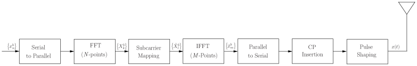
Figure 1: SC-FDMA signal generation.

Fig. 1 shows the SC-FDMA signal generation scheme. The data symbols of the $b$-th input block $\left\{x_{n}^{b}\right\}_{n=0}^{N-1}$ correspond either to a phase-shift-keying (PSK) or a quadrature amplitude modulation (QAM) signal constellation. The serially modulated data symbols are then converted into $N$ parallel data streams, and passed through an $N$-point fast Fourier transform (FFT) block, which generates the frequency domain symbols $\left\{X_{k}^{b}\right\}_{k=0}^{N-1}$. Then, the output of the FFT is passed through the subcarrier mapping block. This assigns the $\left\{X_{k}^{b}\right\}_{k=0}^{N-1}$ symbols to $M\geq N$ subcarriers, usually in a localized mode (LFDMA) [17]. Note that $M=NQ$, with $Q$ as the expansion factor, and the unoccupied subcarriers are set to zero. The output symbols in LFDMA, $\{\tilde{X}_{l}^{b}\}_{l=0}^{M-1}$, are frequency domain samples; these are passed through an $M$-point inverse FFT (IFFT), yielding the time domain samples $\left\{\tilde{x}_{m}^{b}\right\}_{m=0}^{M-1}$. Let $m=Qn+q$, with $n=0,...,N-1$ and $q=0,...,Q-1$. Then, the time domain samples can be expressed as [17]

$$\tilde{x}_{m}^{b}=\begin{cases}\begin{array}[]{l}\frac{1}{Q}{x^{b}_{n}},\\ \\ \frac{\left(1-e^{j\frac{2\pi q}{Q}}\right)}{QN}\overset{N-1}{\underset{p=0}{\sum}}\frac{x_{p}^{b}}{1-e^{j2\pi\left(\frac{\left(n-p\right)}{N}+\frac{q}{QN}\right)}},\end{array}&\begin{array}[]{c}q=0,\\ \\ q\neq 0.\end{array}\end{cases}$$ (1)

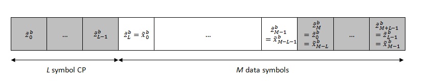
Figure 2: SC-FDMA block with CP.

From (1), one can see that the time-domain LFDMA signal samples consist of copies of the input time symbols scaled by a factor of 1/${Q}$ for the $N$-multiple sample positions; between these positions, the signal samples are the weighted sums of the time symbols in the input block.

To combat the inter-symbol interference caused by the channel delay spread, a cyclic prefix (CP) of $L$ samples is added at the beginning of every $M$ samples $(L<M)$ for each block. According to the standards [17, 18], $L$ is considered a multiple integer of $Q$. A root raised cosine (RRC) filter is used to pulse shape the SC-FDMA signal [17]. The structure of an SC-FDMA block with CP is presented in Fig. 2, where $\tilde{z}_{u}^{b}$ represents the symbol transmitted within the $u$-th symbol period of block $b$, $u=0,...,M+L-1$. The symbol $\tilde{z}_{u}^{b}$ is expressed as

$$\tilde{z}_{u}^{b}=\begin{cases}\begin{array}[]{c}\tilde{x}_{M-L+u}^{b},\\ \\ \tilde{x}_{u-L}^{b},\end{array}&\begin{array}[]{c}u=0,...,L-1,\\ \\ u=L,...,M+L-1.\end{array}\end{cases}$$ (2)

Hence, the received noise-free SC-FDMA signal can be expressed as

$$r(t)=\sum_{b=-\infty}^{\infty}\left[\sum_{u=0}^{M+L-1}\tilde{z}_{u}^{b}g(t-uT-b(M+L)T)\right],$$ (3)

where $g(t)$ represents the pulse shape and $T$ is the symbol duration.

III Second-order Cyclostationarity of SC-FDMA Signals

III-A Definitions

A random process $r(t)$ is said to be second-order cyclostationary if its mean and time-varying autocorrelation function (AF) are almost periodic functions of time [19]. The latter is expressed as a Fourier series [19]

$$c_{r}(t,\tau)=\textrm{E}[r(t)r^{*}(t-\tau)]=\sum_{\beta\in\kappa}c_{r}(\beta,\tau)e^{j2\pi\beta t},$$ (4)

where $\textrm{E}\left[.\right]$ represents the expectation operator, the superscript * denotes complex conjugation, and $c_{r}(\beta,\tau)$ is the CAF at CF $\beta$ and delay $\tau,$ which can be expressed as [19]

$$c_{r}(\beta,\tau)=\lim_{I\rightarrow\infty}I^{-1}\int_{-I/2}^{I/2}c_{r}(t,\tau)e^{-j2\pi\beta t}\,dt,$$ (5)

and $\kappa=\{\beta:\,c_{r}(\beta,\tau)\neq 0\}$ represents the set of CFs.

For a discrete-time signal $r(u)$ obtained by periodically sampling the continuous-time signal $r(t)$ at rate $f_{s},$ the CAF at CF $\tilde{\beta}$ and delay $\tilde{\tau}$ is given by [19]

$$c_{r}(\tilde{\beta},\tilde{\tau})=c_{r}(\beta f_{s}^{-1},\tau f_{s}),$$ (6)

where $\tilde{\beta}=\beta f_{s}^{-1}$ and $\tilde{\tau}=\tau f_{s}$.

The estimator of CAF at CF $\tilde{\beta}$ and delay $\tilde{\tau}$, based on $U_{s}$ samples, is given by [19]

$$\hat{c}_{r}(\tilde{\beta},\tilde{\tau})={U_{s}}^{-1}\sum_{u=0}^{U_{s}-1}r(u)r^{*}(u-\tilde{\tau})e^{-j2\pi\tilde{\beta}u}.$$ (7)

III-B Analytical Expressions of AF, CAF and Set of CFs for the SC-FDMA Signals

By using (3) and (4), the AF of the SC-FDMA signals can be written as

$$\begin{array}[]{ll}c_{r}(t,\tau)&=\overset{\infty}{\underset{b_{1}=-\infty}{\sum}}\overset{\infty}{\underset{b_{2}=-\infty}{\sum}}\overset{M+L-1}{\underset{u_{1}=0}{\sum}}\overset{M+L-1}{\underset{u_{2}=0}{\sum}}\textrm{E}\left[\tilde{z}_{u_{1}}^{b_{1}}(\tilde{z}_{u_{2}}^{b_{2}})^{*}\right]\\ &\times g(t-u_{1}T-b_{1}(M+L)T)\\ &\times g^{*}(t-u_{2}T-b_{2}(M+L)T-\tau).\end{array}$$ (8)

Further, through cumbersome mathematical calculations, one can show that the analytical closed form expression of the AF is given as:

$$\bullet\textrm{ for }{\tau}=\pm{\tau}_{s},\>0\leq{\tau}_{s}<T,{\color[rgb]{1,1,1}............................................................................................}\\ c_{r}(t;{\tau})=\left(\frac{T-{\tau}_{s}}{4T}+\frac{{\tau}_{s}}{2NT}\frac{1}{1-e^{j\pi\frac{1}{N}}}\right)c_{x}\left[g(t)g^{*}(t)\right]\\ \otimes\overset{\infty}{\underset{k=-\infty}{\sum}}\delta(t-kT),{\color[rgb]{1,1,1}...............................}$$ (9a)

$$\bullet\textrm{ for }{\tau}={\mu}T+\textrm{sgn}(\mu){\tau}_{s},\>\mu=\pm 1,\pm 3,\ldots,\\ \pm(M-L-1),\>0\leq{\tau}_{s}<T,\\ c_{r}(t;{\tau})=\frac{T-{\tau}_{s}}{T}A(\mu)\left[g(t)g^{*}(t)\right]\otimes\overset{\infty}{\underset{k=-\infty}{\sum}}\delta(t-kT),\\ \textrm{ where }A(\mu)=\frac{c_{x}}{2N}\frac{1}{1-e^{j\pi\frac{\mid\mu\mid}{N}}},{\color[rgb]{1,1,1}...............................}$$ (9b)

$$\bullet\textrm{ for }{\tau}={\mu}T+\textrm{sgn}(\mu){\tau}_{s},\>\mu=\pm 2,\pm 4,\ldots,\\ \pm(M-L),\>0\leq{\tau}_{s}<T,\\ c_{r}(t;{\tau})=\frac{{\tau}_{s}}{T}A(\mu+1)\left[g(t)g^{*}(t)\right]\otimes\overset{\infty}{\underset{k=-\infty}{\sum}}\delta(t-kT),$$ (9c)

$$\bullet\textrm{ for }{\tau}={\mu}T+\textrm{sgn}(\mu){\tau}_{s},\>\mu=\pm M,\>0\leq{\tau}_{s}<T,\\ c_{r}(t;{\tau})=\left(\frac{T-{\tau}_{s}}{4T}+\frac{{\tau}_{s}}{2NT}\frac{1}{1-e^{\pm j\pi\frac{1}{N}}}\right)\\ \hskip 28.45274pt\times c_{x}\overset{L-1}{\underset{u=0}{\sum}}\left[g(t-uT)g^{*}(t-uT)\right]{\color[rgb]{1,1,1}..}\\ \otimes\overset{\infty}{\underset{b=-\infty}{\sum}}\delta(t-b(M+L)T),{\color[rgb]{1,1,1}.........}$$ (9d)

$$\bullet\textrm{ for }{\tau}={\mu}T+\textrm{sgn}(\mu){\tau}_{s},\>\mu=\pm(M-L+1),\\ \pm(M-L+3),\ldots,\pm(M+L-1),0\leq{\tau}_{s}<T,\\ c_{r}(t;{\tau})=\frac{T-{\tau}_{s}}{T}A(\mu)\overset{L-1}{\underset{u=0}{\sum}}\left[g(t-uT)g^{*}(t-uT)\right]\\ \otimes\overset{\infty}{\underset{b=-\infty}{\sum}}\delta(t-b(M+L)T),{\color[rgb]{1,1,1}...............}$$ (9e)

$$\bullet\textrm{ for }{\tau}={\mu}T+\textrm{sgn}(\mu){\tau}_{s},\>\mu=\pm(M-L+2),\ldots,\\ \pm(M-2),\pm(M+2),\ldots\pm(M+L-2),0\leq{\tau}_{s}<T,{\color[rgb]{1,1,1}.......................................................................................}\\ c_{r}(t;{\tau})=\frac{{\tau}_{s}}{T}A(\mu+1)\overset{L-1}{\underset{u=0}{\sum}}\left[g(t-uT)g^{*}(t-uT)\right]\\ \otimes\overset{\infty}{\underset{b=-\infty}{\sum}}\delta(t-b(M+L)T),{\color[rgb]{1,1,1}...............}$$ (9f)

$$\bullet\textrm{ otherwise }\\ c_{r}(t;{\tau})=0.{\color[rgb]{1,1,1}................................................}$$ (9g)

In the following, we provide the proof for the zero-delay case for illustration. The same procedure is applicable to other cases, as one can see from [20]; details are not included here due to the space considerations.

Proof:

From (8), one can notice that $c_{r}(t,0)$ has non-zero significant values when $b_{1}=b_{2}=b$ (the same data block) and $u_{1}=u_{2}=u$ (the same symbol within a block). Based on this observation, (8) can be expressed as

$$\begin{array}[]{lll}c_{r}(t;0)=&\displaystyle\sum_{b=-\infty}^{\infty}\sum_{u=0}^{M+L-1}\textrm{E}\left[\tilde{z}_{u}^{b}(\tilde{z}_{u}^{b})^{*}\right]\\ &\times g(t-uT-b(M+L)T)\\ &\times g^{*}(t-uT-b(M+L)T).\end{array}$$ (10)

Furthermore, by emphasizing the summation over the CP symbols, and considering $u$ odd and $u$ even, (10) is expressed as

$$\begin{array}[]{ll}c_{r}(t;0)=&\overset{\infty}{\underset{b=-\infty}{\sum}}(\overset{L-1}{\underset{\underset{\textrm{even}}{u=0}}{\sum}}\textrm{E}\left[\tilde{z}_{u}^{b}\left(\tilde{z}_{u}^{b}\right)^{*}\right]g(t-uT-b(M+L)T)\\ &\times g^{*}(t-uT-b(M+L)T))+\overset{\infty}{\underset{b=-\infty}{\sum}}(\textrm{ }\overset{L-1}{\underset{\underset{\textrm{odd}}{u=0}}{\sum}}\textrm{E}\left[\tilde{z}_{u}^{b}\left(\tilde{z}_{u}^{b}\right)^{*}\right]\\ &\times g(t-uT-b(M+L)T)g^{*}(t-uT-b(M+L)T))\\ &+\overset{\infty}{\underset{b=-\infty}{\sum}}(\textrm{ }\overset{M+L-1}{\underset{\underset{\textrm{even}}{u=L}}{\sum}}\textrm{E}\left[\tilde{z}_{u}^{b}\left(\tilde{z}_{u}^{b}\right)^{*}\right]g(t-uT-b(M+L)T)\\ &\times g^{*}(t-uT-b(M+L)T))+\overset{\infty}{\underset{b=-\infty}{\sum}}(\textrm{ }\overset{M+L-1}{\underset{\underset{\textrm{odd}}{u=L}}{\sum}}\textrm{E}\left[\tilde{z}_{u}^{b}\left(\tilde{z}_{u}^{b}\right)^{*}\right]\\ &\times g(t-uT-b(M+L)T)g^{*}(t-uT-b(M+L)T)).\end{array}$$ (11)

Henceforth, we refer to the first, second, third, and fourth terms in the right hand side of (11) as $\mathbb{\mathfrak{c}}_{r}^{(1)}(t;0)$, $\mathbb{\mathfrak{c}}_{r}^{(2)}(t;0)$, $\mathbb{\mathfrak{c}}_{r}^{(3)}(t;0)$, and $\mathbb{\mathfrak{c}}_{r}^{(4)}(t;0)$, respectively. We consider each of these terms, starting with the last two. As such, with $m=u-L$ and using (2), $\mathbb{\mathfrak{c}}_{r}^{(3)}(t;0)$ becomes

$$\begin{array}[]{ll}\mathbb{\mathfrak{c}}_{r}^{(3)}(t;0)=&\overset{\infty}{\underset{b=-\infty}{\sum}}\overset{M-1}{\underset{\underset{\textrm{even}}{m=0}}{\sum}}\textrm{E}\left[\tilde{x}_{m}^{b}\left(\tilde{x}_{m}^{b}\right)^{*}\right]\\ &\times g(t-(m+L)T-b(M+L)T)\\ &\times g^{*}(t-(m+L)T-b(M+L)T).\end{array}$$ (12)

By considering that $m=2n$, $n=0,...,N-1$, and by replacing (1) into (12) with $Q=2$ , $\mathbb{\mathfrak{c}}_{r}^{(3)}(t;0)$ becomes

$$\begin{array}[]{l}\mathbb{\mathfrak{c}}_{r}^{(3)}(t;0)=\frac{c_{x}}{4}\overset{\infty}{\underset{b=-\infty}{\sum}}\overset{M-1}{\underset{\underset{\textrm{even}}{m=0}}{\sum}}g(t-(m+L)T-b(M+L)T)\\ \hskip 39.83368pt\times g^{*}(t-(m+L)T-b(M+L)T),\end{array}$$ (13)

where $c_{x}=\textrm{E}[x_{n}^{b}(x_{n}^{b})^{*}]$ represents the correlation corresponding to the points in the signal constellation.

Similarly, with $m=u-L$ and using (2), $\mathbb{\mathfrak{c}}_{r}^{(4)}(t;0)$ becomes

$$\begin{array}[]{ll}\mathbb{\mathfrak{c}}_{r}^{(4)}(t;0)=&\overset{\infty}{\underset{b=-\infty}{\sum}}\overset{M-1}{\underset{\underset{\textrm{odd}}{m=0}}{\sum}}\textrm{E}\left[\tilde{x}_{m}^{b}\left(\tilde{x}_{m}^{b}\right)^{*}\right]\\ &\times g(t-(m+L)T-b(M+L)T)\\ &\times g^{*}(t-(m+L)T-b(M+L)T).\end{array}$$ (14)

By considering that $m=2n+1$, $n=0,...,N-1$, and by replacing (1) into (14) with $Q=2$ ³, $\mathbb{\mathfrak{c}}_{r}^{(4)}(t;\tau)$ becomes

$$\begin{array}[]{l}\mathbb{\mathfrak{c}}_{r}^{(4)}(t;0)=\overset{\infty}{\underset{b=-\infty}{\sum}}\overset{M-1}{\underset{\underset{\textrm{odd}}{m=0}}{\sum}}\left(\frac{1}{2N}\left(1-e^{j\pi}\right)\right)^{2}\\ \hskip 28.45274pt\times\textrm{E}\left[\overset{N-1}{\underset{p=0}{\sum}}\frac{x_{p}^{b}(x_{p}^{b})^{*}}{(1-e^{j2\pi(\frac{\left(n-p\right)}{N}+\frac{1}{2N})})(1-e^{-j2\pi(\frac{\left(n-p\right)}{N}+\frac{1}{2N})})}\right]\\ \hskip 28.45274pt\times g(t-(m+L)T-b(M+L)T)\\ \hskip 28.45274pt\times g^{*}(t-(m+L)T-b(M+L)T))\\ \qquad\quad\quad=\frac{c_{x}}{2N^{2}}\overset{\infty}{\underset{b=-\infty}{\sum}}\overset{M-1}{\underset{\underset{\textrm{odd}}{m=0}}{\sum}}\left[\overset{N-1}{\underset{p=0}{\sum}}\frac{1}{1-\textrm{cos}(\pi(\frac{2n-2p+1}{N}))}\right]\\ \hskip 28.45274pt\times g(t-(m+L)T-b(M+L)T)\\ \hskip 28.45274pt\times g^{*}(t-(m+L)T-b(M+L)T).\end{array}$$ (15)

By evaluating the summation $\overset{N-1}{\underset{p=0}{\sum}}\frac{1}{1-\textrm{cos}(\pi(\frac{2n-2p+1}{N}))}$ numerically, one finds that it equals ${N^{2}}$/2. Therefore, (15) becomes

$$\begin{array}[]{l}\mathbb{\mathfrak{c}}_{r}^{(4)}(t;0)=\frac{c_{x}}{4}\displaystyle\sum_{b=-\infty}^{\infty}\sum_{\underset{\textrm{odd}}{m=0}}^{M-1}g(t-(m+L)T-b(M+L)T)\\ \hskip 36.98866pt\times g^{*}(t-(m+L)T-b(M+L)T).\end{array}$$ (16)

With $m=M-L+u$, using (2), and following the same procedure as for $\mathbb{\mathfrak{c}}_{r}^{(3)}(t;0)$ and $\mathbb{\mathfrak{c}}_{r}^{(4)}(t;0)$, one can easily show that

$$\begin{array}[]{l}\mathbb{\mathfrak{c}}_{r}^{(1)}(t;0)=\frac{c_{x}}{4}\displaystyle\sum_{b=-\infty}^{\infty}\sum_{\underset{\textrm{odd}}{m=M-L}}^{M-1}g(t-(m-M+L)T\\ -b(M+L)T)g^{*}(t-(m-M+L)T-b(M+L)T).\end{array}$$ (17)

and

$$\begin{array}[]{l}\mathbb{\mathfrak{c}}_{r}^{(2)}(t;0)=\frac{c_{x}}{4}\displaystyle\sum_{b=-\infty}^{\infty}\sum_{\underset{\textrm{odd}}{m=M-L}}^{M-1}g(t-(m-M+L)T\\ -b(M+L)T)g^{*}(t-(m-M+L)T-b(M+L)T).\end{array}$$ (18)

Finally, by substituting (13), (16), (17), and (18), and using $u=m-M+L$ in the expressions of $\mathbb{\mathfrak{c}}_{r}^{(1)}(t;\tau)$ and $\mathbb{\mathfrak{c}}_{r}^{(2)}(t;\tau)$ and $u=m+L$ in the expressions of $\mathbb{\mathfrak{c}}_{r}^{(3)}(t;\tau)$ and $\mathbb{\mathfrak{c}}_{r}^{(4)}(t;\tau)$, (11) becomes

$$\begin{array}[]{l}c_{r}(t;0)=\frac{c_{x}}{4}\displaystyle\sum_{b=-\infty}^{\infty}\sum_{u=0}^{M+L-1}g(t-uT-b(M+L)T)\\ \hskip 32.72049pt\times g^{*}(t-uT-b(M+L)T).\end{array}$$ (19)

With $k=u+b(M+L)$, $c_{r}(t;0)$ can be further written as

$$c_{r}(t;0)=\frac{c_{x}}{4}\left[g(t)g^{*}(t)\right]\otimes\overset{\infty}{\underset{k=-\infty}{\sum}}\delta(t-kT).$$ (20)

∎

By taking the Fourier transform of (9) with respect to $t$, one can easily obtain the CFs, and further using (4), the CAF at CF $\beta$ and delay $\tau$ can be expressed as

$$\bullet\textrm{ for }{\tau}=\pm{\tau}_{s},\>0\leq{\tau}_{s}<T,\textrm{ and }{\beta}=kT^{-1},\,k\textrm{ integer},{\color[rgb]{1,1,1}............................................................................................}\\ c_{r}({\beta};{\tau})=\left(\frac{T-{\tau}_{s}}{4T}+\frac{{\tau}_{s}}{2NT}\frac{1}{1-e^{j\pi\frac{1}{N}}}\right)c_{x}{T^{-1}}\\ \hskip 36.98866pt\times\int_{-\infty}^{\infty}\left[g(t)g^{*}(t)\right]e^{-j2\pi{\beta}t}dt,{\color[rgb]{1,1,1}.................}$$ (21a)

$$\bullet\textrm{ for }{\tau}={\mu}T+\textrm{sgn}(\mu){\tau}_{s},\>\mu=\pm 1,\pm 3,\ldots,\\ \pm(M-L-1),\>0\leq{\tau}_{s}<T,\textrm{ and }{\beta}=kT^{-1},\,k\textrm{ integer},\\ c_{r}({\beta};{\tau})=\frac{T-{\tau}_{s}}{T}A(\mu){T^{-1}}\int_{-\infty}^{\infty}\left[g(t)g^{*}(t)\right]e^{-j2\pi{\beta}t}dt,$$ (21b)

$$\bullet\textrm{ for }{\tau}={\mu}T+\textrm{sgn}(\mu){\tau}_{s},\>\mu=\pm 2,\pm 4,\ldots,\\ \pm(M-L),\>0\leq{\tau}_{s}<T,\textrm{ and }{\beta}=kT^{-1},\,k\textrm{ integer},\\ c_{r}({\beta};{\tau})=\frac{{\tau}_{s}}{T}A(\mu+1){T^{-1}}\int_{-\infty}^{\infty}\left[g(t)g^{*}(t)\right]e^{-j2\pi{\beta}t}dt,$$ (21c)

$$\bullet\textrm{ for }{\tau}={\mu}T+\textrm{sgn}(\mu){\tau}_{s},\>\mu=\pm M,\>0\leq{\tau}_{s}<T,\\ \textrm{ and }{\beta}=b\left[(M+L)T\right]^{-1},\,b\textrm{ integer},\\ c_{r}({\beta};{\tau})=(\frac{T-{\tau}_{s}}{4T}+\frac{{\tau}_{s}}{2NT}\frac{1}{1-e^{\pm j\pi\frac{1}{N}}})c_{x}{\left[(M+L)T\right]^{-1}}\\ \hskip 36.98866pt\times\int_{-\infty}^{\infty}\overset{L-1}{\underset{u=0}{\sum}}\left[g(t-uT)g^{*}(t-uT)\right]e^{-j2\pi{\beta}t}dt,$$ (21d)

$$\bullet\textrm{ for }{\tau}={\mu}T+\textrm{sgn}(\mu){\tau}_{s},\>\mu=\pm(M-L+1),\\ \pm(M-L+3),\ldots,\pm(M+L-1),0\leq{\tau}_{s}<T,\\ \textrm{ and }{\beta}=b\left[(M+L)T\right]^{-1},\,b\textrm{ integer},{\color[rgb]{1,1,1}.....................................................................................}\\ c_{r}({\beta};{\tau})=\frac{T-{\tau}_{s}}{T}A(\mu){\left[(M+L)T\right]^{-1}}{\color[rgb]{1,1,1}.........................................................................................}\\ \hskip 36.98866pt\times\int_{-\infty}^{\infty}\overset{L-1}{\underset{u=0}{\sum}}\left[g(t-uT)g^{*}(t-uT)\right]e^{-j2\pi{\beta}t}dt,$$ (21e)

$$\bullet\textrm{ for }{\tau}={\mu}T+\textrm{sgn}(\mu){\tau}_{s},\>\mu=\pm(M-L+2),\ldots,\\ \pm(M-2),\pm(M+2),\ldots\pm(M+L-2),0\leq{\tau}_{s}<T,\\ \textrm{ and }{\beta}=b\left[(M+L)T\right]^{-1},\,b\textrm{ integer},{\color[rgb]{1,1,1}............................................................................}\\ c_{r}({\beta};{\tau})=\frac{{\tau}_{s}}{T}A(\mu+1){\left[(M+L)T\right]^{-1}}\\ \hskip 34.14322pt\times\int_{-\infty}^{\infty}\overset{L-1}{\underset{u=0}{\sum}}\left[g(t-uT)g^{*}(t-uT)\right]e^{-j2\pi{\beta}t}dt,$$ (21f)

$$\bullet\textrm{ otherwise }\\ c_{r}({\beta};{\tau})=0.{\color[rgb]{1,1,1}................................................}$$ (21g)

The analytical closed-form expression for the CAF of the discrete-time SC-FDMA signals $r(n)=$ $r(t)|$ ${}_{t=nf_{s}}$, $f_{s}=\rho/T$, with $\rho$ as the oversampling factor, can be straightforwardly obtained from (21) by replacing $\beta$ with $\tilde{\beta}f_{s}$ and $\tau$ with $\tilde{\tau}/f_{s}$, according to (6). Note that this expression is not provided here due to space considerations.

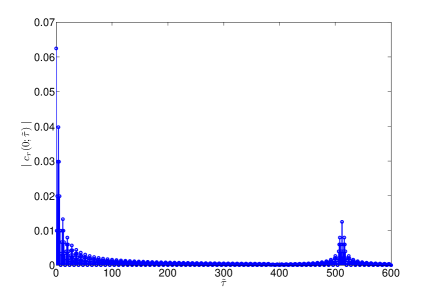
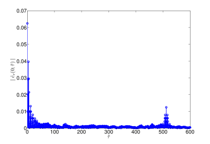
Figure 3: The CAF magnitude at zero CF ($\tilde{\beta}=0$) versus positive delays, $\tilde{\tau}$: (a) theoretical and (b) simulation results.

In the following, theoretical and simulation results are presented for the CAF magnitude of the LTE SC-FDMA signals in the absence of noise for different delays and CFs. The parameters of the LTE SC-FDMA signals are set as in Section V. A, with long CP, and the observation time is 20 ms. Fig. 3 shows the magnitude of the theoretical and estimated CAF magnitude at zero CF versus positive delays. Additionally, Fig. 4 depicts the CAF magnitude at zero delay versus CFs. From these results, one can easily see that the theoretical findings are in agreement with the simulation results. Note that the non-zero CAF values obtained from simulations, which are theoretically zero, are due to a finite observation time; however, they are not statistically significant.

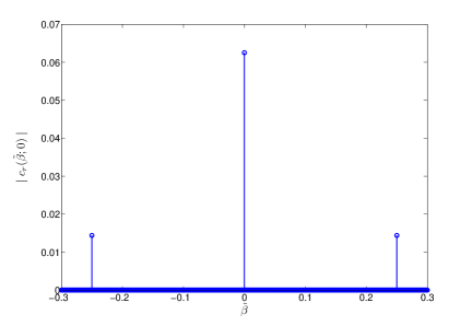
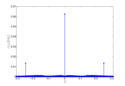
Figure 4: The CAF magnitude at zero delay ($\tilde{\tau}=0$) versus CF, $\tilde{\beta}$: (a) theoretical and (b) simulation results.

IV Proposed Algorithm for the Detection of the LTE SC-FDMA Signals

Here, results obtained in Section III for the CAF of the LTE SC-FDMA signals are exploited to develop a cyclostationarity-based algorithm for their detection. We first introduce the SC-FDMA signal features, and then describe the test used for decision-making and the proposed algorithm, as well as discuss its computational complexity.

IV-A Signal Feature Used for Detection

The SC-FDMA signals are detected in the frequency bands allocated to the LTE system [21]; accordingly, the values of $M$ and $N$ are known. The signal is down-converted and oversampled, and the baseband discrete-time signal, $r(u),\,0\leq u\leq U_{s}-1$, is exploited for detection. Based on the theoretical results presented in Section III, one can see that the CAF magnitude of the received LTE SC-FDMA has the following properties:

• It has non-zero values at zero CF and for delays around $\pm\rho M$, with the latter due to the existence of the CP.

• It is non-zero at CFs equal to $\pm\rho^{-1}$ and for delays around zero.

These particular properties are exploited for the LTE SC-FDMA signal detection. Under hypothesis $\mathcal{H}_{1}$, we assume that the LTE SC-FDMA is present, while under $\mathcal{H}_{0}$ it is not.

IV-B Cyclostationarity Test Used for Decision-Making

Based on the underlying theory of the cyclostationarity test introduced in [22], which verifies if CAF has a CF at $\tilde{\beta}$ for delay $\tilde{\tau}$, a test for two CFs ($\tilde{\beta_{1}}=0$ and $\tilde{\beta_{2}}=\rho^{-1}$) and two delays ($\tilde{\tau}_{1}=\rho M$ and $\tilde{\tau}_{2}=0$) is developed, such that the above mentioned properties of the LTE SC-FDMA signals are exploited.

The test used for decision-making is as follows:

• The CAF of the received signal $r(u)$ is estimated (from $U_{s}$ samples) at each tested frequency $\tilde{\beta_{i}}$ and delay $\tilde{\tau}_{i}$, $i=1,\,2,$ and a vector $\hat{c}_{i}$ is formed as

$$\hat{c}_{i}=[\textrm{Re}\{\hat{c}_{r}(\tilde{\beta_{i}};\tilde{\tau}_{i})\}\,\textrm{Im}\{\hat{c}_{r}(\tilde{\beta}_{i};\tilde{\tau}_{i})\}],$$ (22)

where $\textrm{Re }\{.\}$ and $\textrm{Im }\{.\}$ are the real and the imaginary parts, respectively.

• A statistic $\Psi_{i}$ , $i=1,\,2,$ is computed for each tested frequency $\tilde{\beta}_{i}$ and delay $\tilde{\tau}_{i}$ as [22]

$$\Psi_{i}=U_{s}\hat{c}_{i}\hat{\sum}_{i}^{-1}\hat{c}_{i}^{\intercal},$$ (23)

where the superscripts -1 and $\intercal$ denote the matrix inverse and transpose, respectively, and $\hat{\sum}_{i}$ is an estimate of the covariance matrix

$${\sum}_{i}=\left[\begin{array}[]{cc}\textrm{Re}\left\{\frac{\left(Q_{2,0}+Q_{2,1}\right)}{2}\right\}&\textrm{Im}\left\{\frac{\left(Q_{2,0}-Q_{2,1}\right)}{2}\right\}\\ \textrm{Im}\left\{\frac{\left(Q_{2,0}+Q_{2,1}\right)}{2}\right\}&\textrm{Re}\left\{\frac{\left(Q_{2,1}-Q_{2,0}\right)}{2}\right\}\end{array}\right],$$ (24)

with

$$Q_{2,0}=\underset{U_{s\rightarrow\infty}}{\textrm{lim}}U_{s}\textrm{Cum}[\hat{c}_{r}(\tilde{\beta_{i}};\tilde{\tau}_{i}),\hat{c}_{r}(\tilde{\beta_{i}};\tilde{\tau}_{i})],$$ (25)

and

$$Q_{2,1}=\underset{U_{s\rightarrow\infty}}{\textrm{lim}}U_{s}\textrm{Cum}[\hat{c}_{r}(\tilde{\beta_{i}};\tilde{\tau}_{i}),\hat{c}_{r}^{*}(\tilde{\beta_{i}};\tilde{\tau}_{i})].$$ (26)

For a zero-mean process, the covariances $Q_{2,0}$ and $Q_{2,1}$ are given respectively as [22]

$$\begin{array}[]{l}Q_{2,0}=\underset{U_{s\rightarrow\infty}}{lim}U_{s}^{-1}\displaystyle\sum_{l=0}^{U_{s}-1}\sum_{\xi=-\infty}^{\infty}\textrm{Cum}\left[f\left(l;\tilde{\tau}_{i}\right),f\left(l+\xi;\tilde{\tau}_{i}\right)\right]\\ \hskip 128.0374pt\times e^{-j2\pi 2\tilde{\beta_{i}}l}e^{-j2\pi\tilde{\beta_{i}}\xi},\end{array}$$ (27)

and

$$\begin{array}[]{l}Q_{2,1}=\underset{U_{s\rightarrow\infty}}{lim}U_{s}^{-1}\displaystyle\sum_{l=0}^{U_{s}-1}\sum_{\xi=-\infty}^{\infty}\textrm{Cum}\left[f\left(l;\tilde{\tau}_{i}\right),f^{*}\left(l+\xi;\tilde{\tau}_{i}\right)\right]\\ \hskip 128.0374pt\times e^{-j2\pi(-\tilde{\beta_{i}})\xi l},\end{array}$$ (28)

where $f\left(l;\tilde{\tau}_{i}\right)=r(l)r^{*}(l+\tilde{\tau}_{i})$ is the second-order (one-conjugate) lag product.

Moreover, the estimators of the covariance $Q_{2,0}$ and $Q_{2,1}$ are given respectively by [22]

$$\begin{array}[]{l}\hat{Q}_{2,0}=(U_{s}U_{sw})^{-1}\displaystyle\sum_{s=-(U_{sw}-1)/2}^{(U_{sw}-1)/2}W(s)F_{\tilde{\tau}_{i}}(\tilde{\beta_{i}}-sU_{s}^{-1})\\ \hskip 125.19194pt\times F_{\tilde{\tau}_{i}}(\tilde{\beta}_{i}+sU_{s}^{-1}),\end{array}$$ (29)

and

$$\begin{array}[]{l}\hat{Q}_{2,1}=(U_{s}U_{sw})^{-1}\displaystyle\sum_{s=-(U_{sw}-1)/2}^{(U_{sw}-1)/2}W(s)F_{\tilde{\tau}_{i}}^{*}(\tilde{\beta}_{i}+sU_{s}^{-1})\\ \hskip 125.19194pt\times F_{\tilde{\tau}_{i}}(\tilde{\beta}_{i}+sU_{s}^{-1}),\end{array}$$ (30)

where $W(s)$ is a spectral window of length $U_{sw}$ and $F_{\tilde{\tau}_{i}}(\tilde{\beta}_{i})=\overset{U_{s}-1}{\underset{u=0}{\sum}}r(u)r^{*}(u-\tilde{\tau}_{i})e^{-j2\pi\tilde{\beta}_{i}u}$.

• With the test statistics $\Psi_{1}$ and $\Psi_{2}$ calculated based on the estimated CAF at $\tilde{\beta_{1}}=0$ and $\tilde{\tau}_{1}$=$\rho M$ and at $\tilde{\beta_{2}}=\rho^{-1}$ and $\tilde{\tau}_{2}=$0, respectively, we form a new test statistic, $\Upsilon=\Psi_{1}+\Psi_{2}$. For decision-making, we compare $\Upsilon$ against a threshold, $\Gamma$. If $\Upsilon\geq\Gamma,$ we decide that the LTE SC-FDMA is present (hypothesis $\mathcal{H}_{1}$); otherwise, that it is not (hypothesis $\mathcal{H}_{0}$). By using that the statistics $\Psi_{1}$ and $\Psi_{2}$ have asymptotic chi-square distribution with two degrees of freedom [22], it is straightforward to find that $\Upsilon$ asymptotically follows a chi-square distribution with four degrees of freedom. The threshold $\Gamma$ is obtained from the tables of this chi-squared distribution for a given value of the probability of false alarm ($P_{fa}$), i.e., $P_{fa}=\textrm{$P_{r}$}\left\{\Psi\geq\Gamma\mid H_{0}\right\}$ [23]. A summary of the proposed detection algorithm is provided below.

Summary of the proposed detection algorithm

Input: The observed samples $r(u)$, $u=0,...,U_{s}-1,$ and $\rho$, $M$, and target $P_{fa}$.

- Calculate $\hat{c}_{r}(0,\rho M)$ and $\hat{c}_{r}(\rho^{-1},0)$ using (7).

- Calculate $\Psi_{1}$ using $\hat{c}_{r}(0,\rho M)$, according to (23).

- Calculate $\Psi_{2}$ using $\hat{c}_{r}(\rho^{-1},0)$, according to (23).

- Calculate $\Upsilon=\Psi_{1}+\Psi_{2}$.

- Calculate $\Gamma$ based on $P_{fa}$.

if $\Upsilon\geq\Gamma$ then

     - LTE SC-FDMA is present ($\mathcal{H}_{1}$ true).

else

     - LTE SC-FDMA is not present ($\mathcal{H}_{0}$ true).

end if

C. Complexity Analysis of the Proposed Detection Algorithm

The computational complexity of the algorithm is basically determined by the calculation of the test statistic $\Upsilon$, which entitles computation of $\Psi_{1}$ and $\Psi_{2}$. In order to obtain the number of operations required for that, in the following we investigate the complexity of estimating the CAF at $\tilde{\beta}_{i}$ and $\tilde{\tau}_{i}$, $\hat{c}_{r}(\tilde{\beta}_{i},\tilde{\tau}_{i})$, $i=1,2,$. As such, according to (7), the estimation of CAF at $\tilde{\beta}_{1}=0$ and $\tilde{\tau}_{1}={\rho}M$ requires $U_{s}$ complex multiplications and $U_{s}-1$ complex additions, while $2U_{s}$ complex multiplications and $U_{s}-1$ complex additions are required for $\tilde{\beta}_{2}={\rho}^{-1}$ and $\tilde{\tau}_{2}=0$. Furthermore, based on (24), (29), (30), and the expression of $\Psi_{i}$ in (23), one can find that the number of complex multiplications, complex additions, and real operations needed to calculate $\Psi_{i}$ is $(U_{s}/2)log_{2}U_{s}+2U_{sw}$, $U_{s}log_{2}U_{s}+2(U_{sw}-1)$, and $9U_{sw}+26$, respectively. Moreover, by considering $\Psi_{1}$, $\Psi_{2}$, $\Upsilon$, as well as the comparison between $\Gamma$ and $\Upsilon$, and using the fact that a complex multiplication requires 6 floating point operations (flops), a complex addition requires 2 flops, and a real operation requires 1 flop, the total number of flops required by the algorithm equals $10U_{s}log_{2}U_{s}+22U_{s}+50U_{sw}+42$ . For example, with $U_{s}=$64000 (12.8 ms observation time) and $U_{sw}=$ $0.006U_{s}$, the proposed algorithm needs 11,645,343 flops, while with $U_{s}=$32000 (6.4 ms observation time), it requires 5,502,692 flops. Practically speaking, with a microprocessor that can execute up to 79.2 billion flops per second , a decision can be performed in approximately 0.147 ms when the observation time is 12.8 ms and in 0.069 ms when the observation time is 6.4 ms. It is worth noting that the computational time is significantly lower than the observation time. Also, there is a tradeoff between complexity and performance, i.e., a longer observation time will lead to an increased complexity, but also to an improved performance, as it will be shown in Section V.

V Simulation and Experimental Results

V-A Simulation Setup

The performance of the algorithm proposed for the detection of the LTE SC-FDMA signals used in the uplink transmission is investigated here. Unless otherwise mentioned, the following parameter values were employed for the SC-FDMA signals [21]: 1.4 MHz bandwidth, $N=72,$ $M=128,$ $\rho=4$. The subcarrier spacing was set to $\triangle f=15$ kHz, $L$/$M=$1/4 for long CP, and $L$/$M$=10/128 for the first symbol in the slot and $L$/$M=$9/128 for the remaining symbols for short CP. An RRC with 0.35 roll-off factor was employed at the transmit-side and 16-QAM modulation with unit variance was considered. The impairments which affected the received signals were: 500 kHz carrier frequency offset and uniformly distributed phase and timing offsets over [$-\pi,\pi$) and [$0,1$), respectively. We considered the additive white Gaussian noise (AWGN), and ITU-R pedestrian and vehicular A channels [24]. The maximum Doppler frequencies equal 9.72 Hz and 194.44 Hz for the pedestrian and vehicular fading channels, respectively. The out-of-band noise was removed at the receive-side with a 13 order low-pass Butterworth filter, and the SNR was set at the output of this filter. The probability of detection, $P_{d}$, is used as a performance measure; this is estimated based on 1000 Monte Carlo trials. Unless otherwise mentioned, the sensing times of 6.4 ms and 12.8 ms were used, the probability of false alarm was equal to $P_{fa}$= 0.01, and a 16-bit uniform quantizer with an overloading factor of 4 was considered for the analog-to-digital converter (ADC).

V-B Experimental Setup

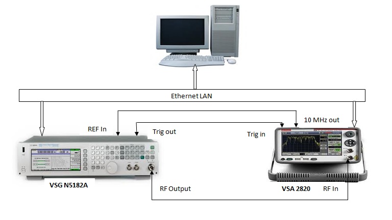
Figure 5: Measurement station.

A measurement station was set up as depicted in Fig. 5. This consists of: 1) a processing and control unit, namely, a personal computer (PC), 2) an Agilent vector signal generator (VSG N5182A), and 3) a Keithley vector signal analyzer (VSA 2080). The three components were interfaced via Ethernet. By using the LTE SC-FDMA signal emulation built into the VSG and the Agilent Studio toolkit, the VSG generated an RF analog signal, which was transmitted to the VSA through a cable. The received analog RF signal was down-converted to intermediate frequency, and then converted to a digital signal, as well as to baseband. Finally, by using the Keithley SignalMeister, the signal captured with the VSA was transferred to the PC, where the detection algorithm was applied. The signal parameters were the same as used in the computer simulations.

V-C Algorithm Performance

The performance of the proposed algorithm is investigated in terms of the probability of detection, $P_{d}$, for the LTE SC-FDMA signals, under various conditions. Results obtained from both computer simulations (black color) and experiments (red color) are shown, with a good agreement between simulation and experimental findings.

In Fig. 6, results for $P_{d}$ versus $P_{fa}$ are presented at different SNRs, for the ITU-R pedestrian A fading channel and with 12.8 ms observation time. Clearly, the detection performance improves with an increase in SNR. For example, with -10 dB SNR, $P_{d}$ approaches 1 at $P_{fa}$ around 0.1, while with -15 dB SNR, this occurs at $P_{fa}$ around 0.35.

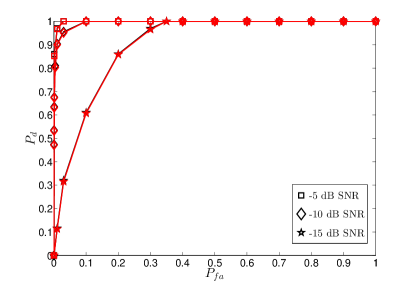
Figure 6: The probability of detection, $P_{d}$, versus $P_{fa}$ for LTE SC-FDMA signals with long CP affected by pedestrian A channel, for different SNRs and with 12.8 ms observation time. Simulation (black color) and experimental (red color) results.

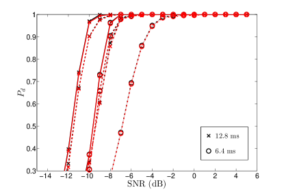
Figure 7: The probability of detection, $P_{d}$, versus SNR for the LTE SC-FDMA signals with long CP affected by AWGN (solid line), pedestrian A (dashed line), and vehicular A (dashed-dot line) channels, respectively. Simulation (black color) and experimental (red color) results.

Fig. 7 shows $P_{d}$ versus SNR for the LTE SC-FDMA signal with long CP, and considering AWGN (solid line), ITU-R pedestrian A (dashed line), and ITU-R vehicular A fading (dashed-dot line) channels, as well as the observation times of 6.4 ms and 12.8 ms. As expected, the best performance is obtained in the AWGN channel, followed by the pedestrian and vehicular A channels. While results achieved in the pedestrian A channel are close to those in AWGN, a longer observation time is required to reach the same performance in the vehicular A channel. Also as expected, $P_{d}$ improves as the observation time increases.

Fig. 8 depicts $P_{d}$ versus SNR for the vehicular A channel, with different observation times. As previously noticed, the detection performance enhances with an increase in the observation time. For example, while $P_{d}$ approaches 1 at $-6$ dB SNR with 12.8 ms observation time, such a performance is achieved at $-12$ dB SNR with 128 ms observation time.

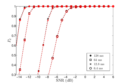
Figure 8: The probability of detection, $P_{d}$, versus SNR for LTE SC-FDMA signals with long CP affected by vehicular A channel, for different observation times. Simulation (black color) and experimental (red color) results.

Fig. 9 presents the detection performance for LTE SC-FDMA signals with long and short CPs for the pedestrian and vehicular A channels. As expected, a reduction in the CP duration adversely affects the performance under the same conditions. This is explained by the reduction in the correlation resulting from the reduced CP duration.

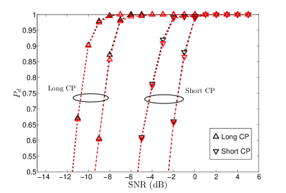
Figure 9: The probability of detection, $P_{d}$, versus SNR for LTE SC-FDMA signals with long and short CP affected by pedestrian A (dashed line) and vehicular A (dashed-dot line) channels, with 12.8 ms observation time. Simulation (black color) and experimental (red color) results.

The effect of the oversampling factor, $\rho$, on $P_{d}$ is shown in Fig. 10; $P_{d}$ is plotted versus SNR for $\rho=2,4,8$, for the pedestrian A channel, with observation times of 6.4 ms and 12.8 ms. As expected, the detection performance improves with an increase in $\rho$ for a certain observation time, as the number of samples increase, which in turn leads to more accurate estimates.

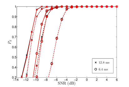
Figure 10: The probability of detection, $P_{d}$, versus SNR for the LTE SC-FDMA signals with long CP affected by pedestrian A channel, with $\rho=8$ (solid line), 4 (dashed line), and 2 (dashed-dot line). Simulation (black color) and experimental (red color) results.

Fig. 11 shows the effect of the quantization error on the performance of the proposed detection algorithm when 8, 12, 16, or 24 bits are respectively used. This error is modeled as an additive noise with uniform distribution over the interval $-\Delta/2$ to $\Delta/2$, where $\Delta$ is the quantization step size which depends on the bit resolution [26]. As can be noticed from Fig. 11, the quantization error does not basically affect the performance. This can be explained, as the proposed algorithm is applied for detecting the presence of LTE SC-FDMA signals rather than detecting the information carried by such signals.

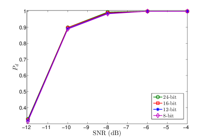
Figure 11: The probability of detection, $P_{d}$, versus SNR for the LTE SC-FDMA signals with long CP affected by pedestrian A channel, with 12.8 ms observation time and for various numbers of quantization bits. ……………………………………………….                                                                                      ………………

Additionally, we investigated the performance of the proposed detection algorithm in the presence of interference, with results shown in Figs. 12-14. We considered multiuser Gaussian interference, as commonly used in the literature [27, 28, 29].

Fig. 12 depicts $P_{d}$ versus SNR for the pedestrian A channel, with 12.8 ms observation time and for different values of the signal-to-interference ratio (SIR). Apparently, the detection performance degrades as the SIR reduces. For example, with SIR = 0 dB, $P_{d}$ approaches one at around SNR=-7 dB, while the same performance is achieved with SIR=-5 dB at SNR=-5 dB. On the other hand, the detection performance degrades significantly with SIR=-10 dB.

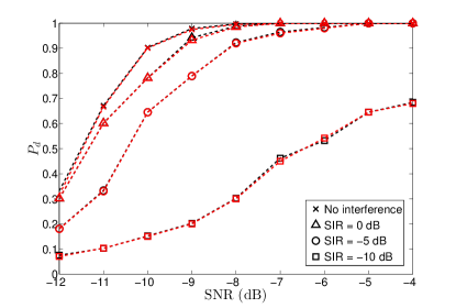
Figure 12: The probability of detection, $P_{d}$, versus SNR for LTE SC-FDMA signals with long CP affected by pedestrian A channel, with 12.8 ms observation time and for different SIRs. Simulation (black color) and experimental (red color) results.

Fig. 13 shows $P_{d}$ versus the observation time at different SIRs, for the pedestrian A channel, and SNR= -10 dB. As expected, the performance improves if the observation interval increases; for example, the detection algorithm fails with SIR=-5 dB and 5 ms observation time, while $P_{d}$ approaches one with 20 ms observation time for the same SIR. Moreover, less observation time is required to approach $P_{d}=1$ for higher SIR; for example, 15 ms is needed at SIR=5 dB, while 20 ms is required at SIR=-5 dB.

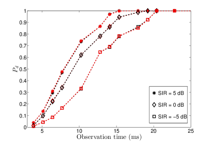
Figure 13: The probability of detection, $P_{d}$, versus the observation time for the LTE SC-FDMA signals with long CP affected by pedestrian A channel, for SNR=-10 dB and different SIRs. Simulation (black color) and experimental (red color) results.

Fig. 14 presents $P_{d}$ versus $P_{fa}$ at different SIRs, for the pedestrian A channel, with 12.8 ms observation time, and SNR=-10 dB. As expected, a better $P_{d}$ is achieved as $P_{fa}$ increases. For example, $P_{d}$ is around 0.93 for $P_{fa}=0.01$, while $P_{d}$ approaches one for $P_{fa}=0.1$ when SIR=5 dB. Apparently, a better detection performance is attained when SIR increases. For example, with SIR=5 dB, $P_{d}$ approaches one at $P_{fa}=0.1$, while the same performance is obtained with SIR=-5 dB at $P_{fa}=0.3$.

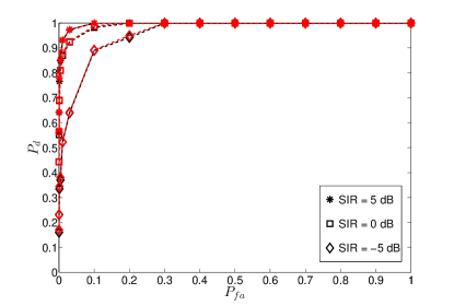
Figure 14: The probability of detection, $P_{d}$, versus $P_{fa}$ for the LTE SC-FDMA signals with long CP affected by pedestrian A channel, with 12.8 ms observation time, for SNR=-10 dB and different SIRs. Simulation (black color) and experimental (red color) results.

VI Conclusion

In this paper, the second-order cyclostationarity of the LTE SC-FDMA signal was studied, and closed form expressions for the corresponding CAF and CFs were derived. Furthermore, based on these findings, an algorithm was developed for the detection of the LTE SC-FDMA signals. Experiments were carried out using computer simulations and signals generated by laboratory equipment to evaluate the performance of the proposed algorithm under diverse scenarios, involving various channel conditions, SNRs, SIRs, and observation times. Results showed that this provides a good performance at low SNRs and with a relatively short observation time, even in the presence of interference. In addition, it requires neither frequency and timing synchronization nor channel estimation. The algorithm can be implemented in real world scenarios, with reduced complexity.

References

- [1] S. Haykin, “Cognitive radio: brain-empowered wireless communications,” IEEE J. Sel. Areas Commun., vol. 23, pp. 201–220, Feb. 2005.
- [2] T. Yucek and H. Arslan, “A survey of spectrum sensing algorithms for cognitive radio applications,” IEEE Commun. Surveys & Tutorials, vol. 11, pp. 116–130, Mar. 2009.
- [3] E. Axell, G. Leus, E. G. Larsson, and H. V. Poor, “Spectrum sensing for cognitive radio: State-of-the-art and recent advances,” IEEE Signal Process. Mag., vol. 29, pp. 101–116, May 2012.
- [4] D. Bao, L. De Vito, and S. Rapuano, “A histogram-based segmentation method for wideband spectrum sensing in cognitive radios,” IEEE Trans. Instrum. Meas., vol. 62, pp. 1900–1908, Jul. 2013.
- [5] K. Barbé and W. Van Moer, “Automatic detection, estimation, and validation of harmonic components in measured power spectra: All-in-one approach,” IEEE Trans. Instrum. Meas., vol. 60, pp. 1061–1069, Mar. 2011.
- [6] O. A. Dobre, A. Abdi, Y. Bar-Ness, and W. Su, “Survey of automatic modulation classification techniques: classical approaches and new trends,” IET Commun., vol. 1, pp. 137–156, Apr. 2007.
- [7] A. Al-Habashna, O. A. Dobre, R. Venkatesan, and D. C. Popescu, “Second-order cyclostationarity of mobile WiMAX and LTE OFDM signals and application to spectrum awareness in cognitive radio systems,” IEEE J. Sel. Topics Sig. Proc., vol. 6, pp. 26–42, Feb. 2012.
- [8] A. Punchihewa, Q. Zhang, O. A. Dobre, C. Spooner, S. Rajan, and R. Inkol, “On the cyclostationarity of ofdm and single carrier linearly digitally modulated signals in time dispersive channels: Theoretical developments and application,” IEEE Trans. Wireless Commun., vol. 9, pp. 2588–2599, Aug. 2010.
- [9] M. Oner and F. Jondral, “On the extraction of the channel allocation information in spectrum pooling systems,” IEEE J. Sel. Areas Commun., vol. 25, pp. 558–565, Apr. 2007.
- [10] F.-X. Socheleau, S. Houcke, P. Ciblat, and A. Aïssa-El-Bey, “Cognitive ofdm system detection using pilot tones second and third-order cyclostationarity,” Elsevier: Signal Processing, vol. 91, pp. 252–268, Feb. 2011.
- [11] K. Kim, C. M. Spooner, I. Akbar, and J. H. Reed, “Specific emitter identification for cognitive radio with application to IEEE 802.11,” in Proc. IEEE GLOBECOM, 2008, pp. 1–5.
- [12] M. Adrat, J. Leduc, S. Couturier, M. Antweiler, and H. Elders-Boll, “2nd order cyclostationarity of OFDM signals: Impact of pilot tones and cyclic prefix,” in Proc. IEEE ICC, 2009, pp. 1–5.
- [13] P. D. Sutton, K. E. Nolan, and L. E. Doyle, “Cyclostationary signatures in practical cognitive radio applications,” IEEE J. Sel. Areas Commun., vol. 26, pp. 13–24, Jan. 2008.
- [14] A. Bouzegzi, P. Ciblat, and P. Jallon, “New algorithms for blind recognition of OFDM based systems,” Elsevier: Signal Processing, vol. 90, pp. 900–913, Mar. 2010.
- [15] D. Grimaldi, S. Rapuano, and L. De Vito, “An automatic digital modulation classifier for measurement on telecommunication networks,” IEEE Trans. Instrum. Meas., vol. 56, pp. 1711–1720, Oct. 2007.
- [16] Q. Zhang, O. A. Dobre, Y. A. Eldemerdash, S. Rajan, and R. Inkol, “Second-order cyclostationarity of BT-SCLD signals: Theoretical developments and applications to signal classification and blind parameter estimation,” IEEE Trans. Wireless Commun., vol. 12, pp. 1501–1511, Apr. 2013.
- [17] H. G. Myung and D. Goodman, Single Carrier FDMA: A New Air Interface For Long Term Evolution. Wiley, 2008, vol. 8.
- [18] J. G. Andrews, A. Ghosh, and R. Muhamed, Fundamentals of WiMAX: Understanding Broadband Wireless Networking. Pearson Education, 2007.
- [19] C. Spooner and W. Gardner, “The cumulant theory of cyclostationary time-series, part i: foundation and part ii: development and applications,” IEEE Trans. Sig. Proc., vol. 42, pp. 3409–3429, Dec. 1994.
- [20] W. Jerjawi, “Second-order Cyclostationarity-based Detection and Classification of LTE SC-FDMA Signals for Cognitive Radio,” Master’s thesis, Memorial University, St. John’s, NL, Canada, 2014.
- [21] Evolved Universal Terrestrial Radio Access (E-UTRA); User Equipment (UE) Radio Transmission and Reception, 3GPP TS 36.101, 2009.
- [22] A. V. Dandawate and G. B. Giannakis, “Statistical tests for presence of cyclostationarity,” IEEE Trans. Sign. Proc., vol. 42, pp. 2355–2369, Sep. 1994.
- [23] M. Abramowitz and I. A. Stegun, Handbook of Mathematical Functions: with Formulas, Graphs, and Mathematical Tables. Courier Dover Publications, 2012.
- [24] A. Molisch, Wireless Communications. Wiley, 2011.
-
[25]
[Online]. Available: http://cp.literature.agilent.com/litweb/pdf/
E4400-90627.pdf. - [26] A. Gersho, “Quantization,” IEEE Commun. Soc. Mag., vol. 15, pp. 16–29, Sep. 1977.
- [27] S. Hayashi and Z.-Q. Luo, “Spectrum management for interference-limited multiuser communication systems,” IEEE Trans. Inf. Theory, vol. 55, pp. 1153–1175, Mar. 2009.
- [28] C. W. Tan, S. Friedland, and S. H. Low, “Spectrum management in multiuser cognitive wireless networks: Optimality and algorithm,” IEEE J. Sel. Areas Commun., vol. 29, pp. 421–430, Feb. 2011.
- [29] D. M. Kalathil and R. Jain, “Spectrum sharing through contracts for cognitive radios,” IEEE Trans. Mobile Comput., vol. 12, pp. 1999–2011, Oct. 2013.