Asymptotically flat multi-black lenses

Abstract

We present an asymptotically flat and stationary multi-black lens solution with bi-axisymmetry of $U(1)\times U(1)$ as a supersymmetric solution in the five-dimensional minimal ungauged supergravity. We show that the spatial cross section of each degenerate Killing horizon admits different lens space topologies of $L(n,1)=S^{3}/{\mathbb{Z}_{n}}$ as well as a sphere $S^{3}$. Moreover, we show that in contrast to the higher dimensional Majumdar-Papapertrou multi-black hole and multi-BMPV black hole spacetimes, the metric is smooth on each horizon even if the horizon topology is spherical.

I Introduction

In recent years, in string theory and the various contexts of AdS/CFT correspondence, higher dimensional black holes and other extended black objects have played an important role Tangherlini:1963bw ; Myers:1986un ; Emparan:2001wn ; Pomeransky:2006bd ; Emparan:2008eg . In particular, physics of asymptotically flat black holes in the five-dimensional minimal supergravity (Einstein-Maxwell-Chern-Simons theory) has been the subject of increased attention, as it describes a low-energy limit of string theory. Various types of black hole solutions in the theory have so far been found, with the help of recent development of solution generating techniques Gauntlett:2002nw ; Bellorin:2006yr ; Bellorin:2007yp ; Gutowski:2005id ; Gauntlett:1998fz ; Grover:2008ih ; Gutowski:2007ai ; Reall:2002bh ; Breckenridge:1996is ; Gibbons:1999uv ; Elvang:2004rt ; Elvang:2004ds ; Elvang:2004xi ; Compere:2009iy ; Gibbons:2013tqa ; Kunduri:2014iga ; Kunduri:2013vka ; Niehoff:2016gbi ; Tomizawa:2012nk ; Mizoguchi:2012vg ; Mizoguchi:2011zj ; Tomizawa:2008qr ; Tomizawa:2008rh ; Matsuno:2008fn ; Tomizawa:2008tj ; Nakagawa:2008rm ; Tomizawa:2007he ; Ishihara:2006pb ; Ishihara:2006iv ; Ishihara:2005dp ; Bena:2004de ; Bena:2007kg ; Bena:2009qv .

The topology theorem for stationary black holes generalized to five dimensions Cai:2001su ; Galloway:2005mf ; Hollands:2007aj ; Hollands:2010qy states that the topology of the spatial cross section of the event horizon is restricted to either a sphere $S^{3}$, a ring $S^{1}\times S^{2}$, or lens spaces $L(p,q)$ $(p,q:$ coprime integers), if one assumes that the spacetime is asymptotically flat and admits three commuting Killing vector fields, a timelike Killing vector field and two axial Killing vector fields under the dominant energy condition. As for the first two cases, one knows the corresponding exact solutions in five-dimensional Einstein theory Myers:1986un ; Emparan:2001wn ; Pomeransky:2006bd and minimal ungauded supergravity theory Breckenridge:1996is ; Elvang:2004rt ; Elvang:2004ds . On the contrary, a regular black hole solution with a lens space topology, at present, has not been found to the five-dimensional vacuum Einstein equation, although a few authors have attempted to construct such a black lens solution by using the combination of the rod diagram and the inverse scattering method Evslin:2008gx ; Chen:2008fa .

Recently, there has been a new development in this field. Asymptotically flat and stationary black lens solutions, whose horizon topology is restricted to $L(2,1)=S^{3}/{\mathbb{Z}}_{2}$, were constructed by Kunduri and Lucietti as supersymmetric solutions to the five-dimensional minimal ungauged supergravity Kunduri:2014kja and $U(1)^{3}$ supergravity Kunduri:2016xbo . Furthermore, the more general black lenses with the horizon topologies of $L(n,1)=S^{3}/{\mathbb{Z}}_{n}\ (n\geq 3)$ were also constructed by one of the present authors in the former theory Tomizawa:2016kjh . The basic strategy to get these supersymmetric black lens solutions is to use the well-known method developed by Gauntlett et al. in Gauntlett:2002nw .

It is well known that the Majumdar-Papapetrou solution to the four dimensional Einstein-Maxwell equation describes an arbitrary number of charged static black holes in an asymptotically flat spacetime by a balance of electromagnetic and gravitational forces Majumdar:1947eu ; Papapetrou:1948jw . Such an asymptotically flat, static multi-black hole solution was perviously generalized to higher dimensional Einstein-Maxwell theories  Myers:1986rx . Furthermore, a multi-black hole solution in a rotational case (this is often called multi-BMPV black hole) was constructed in five-dimensional minimal supergravity Candlish:2009vy . As shown in Welch:1995dh ; Candlish:2007fh ; Candlish:2009vy , in contrast to the four-dimensional Majumdar-Papapetrou solution Hartle:1972ya , these solutions generalized to higher dimensions do not admit smoothness of the metric at horizons, whereas for the concentric multi-black ring solution  Elvang:2004rt , the spacetime is known to be analytic at each event horizon. Therefore, it is not entirely clear whether there does exist a regular multi-black lens solution in higher dimensions, simply because a black lens solution with a single horizon exists.

The purpose of this paper is to construct an exact solution describing an arbitrary number of charged rotating black lenses with smooth horizons as an asymptotically flat and stationary supersymmetric solution in five-dimensional minimal supergravity. This work is essentially based on the previous works of Kunduri:2014kja ; Tomizawa:2016kjh , where the strategy is to use the Gibbons-Hawking space as a hyper-Kähler base space and allow the harmonic functions to have $n$ point sources with appropriate coefficients. We show that by imposing appropriate boundary conditions on the parameters, the $n$ point sources denote degenerate Killing horizons with the topologies of different lens spaces $L(n_{i},1)=S^{3}/Z_{n_{i}}\ (i=1,\cdots,n)$. Moreover, introducing an appropriate coordinate system, we also show that the metric and Maxwell’s field strength are smooth on each horizon in contrast to the higher dimensional Majumdar-Papapetrou solutions and multi-BMPV black hole solution.

This paper is organized as follows: In Sec. II, following the work of Gauntlett et al. Gauntlett:2002nw , we present the supersymmetric solution on the Gibbons-Hawking base space, which describes multi-black lenses in the five-dimensional minimal ungauged supergravity. The solution admits three commuting Killing vector fields, i.e., the stationary Killing vector field, two mutually commuting axial Killing vector fields so that the isometry group of the spacetime is ${\mathbb{R}}\times U(1)\times U(1)$. In Sec. III, we impose the boundary conditions so that the spacetime is asymptotically flat, admits no closed timelike curves (CTCs) on and outside the horizons, neither conical nor curvature singularities appear in the domain of outer communications, and no orbifold singularity and no Dirac-Misner string exists on the axis. Section IV is devoted to study some physical properties of such multiple black lenses. In Sec. V, we summarize our result and discuss further generalization.

II Black lens solution

We would like to consider supersymmetric solutions in the five-dimensional minimal ungauged supergravity, whose bosonic Lagrangian is described by the Einstein-Maxwell-Chern-Simons theory:

$$\mathcal{L}=R\star 1-2F\wedge\star F-\frac{8}{3\sqrt{3}}A\wedge F\wedge F\,,$$ (1)

where $F=dA$ is the Maxwell field. The metric and gauge potential $1$-form are given by

$$ds^{2} = -f^{2}(dt+\omega)^{2}+f^{-1}ds_{M}^{2},$$ (2)

$$A = \frac{\sqrt{3}}{2}\left[f(dt+\omega)-\frac{K}{H}(d\psi+\chi)-\xi\right]\,.$$ (3)

where we choose the hyper-Kähler metric $ds^{2}_{M}$ to be the Gibbons-Hawking metric

$$ds^{2}_{M} = H^{-1}(d\psi+\chi)^{2}+Hdx^{i}dx^{i},$$ (4)

$$d\chi = *dH\,,$$ (5)

where $\{x^{i}\}=(x,y,z)\ (i=1,2,3)$ are Cartesian coordinates on $\mathbb{E}^{3}$ and $\partial/\partial\psi$ is a triholomorphic Killing vector. Furthermore,

$$f^{-1} = H^{-1}K^{2}+L,$$ (6)

$$\omega = \omega_{\psi}(d\psi+\chi)+\hat{\omega},$$ (7)

$$\omega_{\psi} = H^{-2}K^{3}+\frac{3}{2}H^{-1}KL+M,$$ (8)

$$d\hat{\omega} = HdM-MdH+\frac{3}{2}(KdL-LdK),$$ (9)

$$\qquad d\xi = -*dK\,.$$ (10)

Here $H,K,L,M$ are harmonic functions on $\mathbb{E}^{3}$, where it should be noted that there exists a gauge freedom of redefining harmonic functions Bena:2005ni

$$K\to K+aH,\qquad L\to L-2aK-a^{2}H,\qquad M\to M-\frac{3}{2}aL+\frac{3}{2}a^{2}K+\frac{1}{2}a^{3}H,$$ (11)

where $a$ is an arbitrary constant. In fact, under the transformation (11), ($f,\omega_{\psi},\chi$) remain invariant, whereas the 1-form $\xi$ undergoes a change as $\xi\to\xi-a\chi$. Since this transformation merely amounts to the gauge transformation $A\to A+ad\psi$, the transformation (11) makes the bosonic sector invariant.

Following the papers on supersymmetric black lenses in Kunduri:2014kja and Tomizawa:2016kjh , we consider the next harmonic functions with $n$ point sources

$$H = \sum_{i=1}^{n}\frac{h_{i}}{r_{i}}:=\sum_{i=1}^{n}\frac{n_{i}}{r_{i}},$$ (12)

$$M = m_{0}+\sum_{i=1}^{n}\frac{m_{i}}{r_{i}},$$ (13)

$$K = \sum_{i=1}^{n}\frac{k_{i}}{r_{i}},$$ (14)

$$L = l_{0}+\sum_{i=1}^{n}\frac{l_{i}}{r_{i}}.$$ (15)

Here, each $n_{i}$ takes not only positive but also negative integers ($n_{i}=\pm 1,\pm 2,\cdots$), and $r_{i}:=|{\bm{r}}-{\bm{r}_{i}}|=\sqrt{(x-x_{i})^{2}+(y-y_{i})^{2}+(z-z_{i})^{2}}$ with constants $(x_{i},y_{i},z_{i})$.

From Eq. (5), (9) and (10), the 1-forms ($\chi,\xi,\hat{\omega}$) are determined as

$$\chi = \sum_{i=1}^{n}h_{i}\tilde{\omega}_{i},$$ (16)

$$\xi =- \sum_{i=1}^{n}k_{i}\tilde{\omega}_{i},$$ (17)

$$\hat{\omega} = \sum_{i,j=1(i\not=j)}^{n}\left(h_{i}m_{j}+\frac{3}{2}k_{i}l_{j}\right)\hat{\omega}_{ij}-\sum_{i=1}^{n}\left(m_{0}h_{i}+\frac{3}{2}l_{0}k_{i}\right)\tilde{\omega}_{i}+c,$$ (18)

where $c$ is a constant and the 1-forms $\tilde{\omega}_{i}$ and $\hat{\omega}_{ij}$ ($i\not=j$) on ${\mathbb{E}}^{3}$ are, respectively,

$$\tilde{\omega}_{i} = \frac{z-z_{i}}{r_{i}}\frac{(x-x_{i})dy-(y-y_{i})dx}{(x-x_{i})^{2}+(y-y_{i})^{2}},$$ (19)

$$\hat{\omega}_{ij} = -\frac{({\bm{r}}-{\bm{r}}_{i})\cdot({\bm{r}}-{\bm{r}}_{j})}{r_{i}r_{j}}\frac{\left[({\bm{r}}_{i}-{\bm{r}}_{j})\times({\bm{r}}-\frac{{\bm{r}_{i}}+{\bm{r}_{j}}}{2})\right]_{k}dx^{k}}{\left|({\bm{r}}_{i}-{\bm{r}}_{j})\times({\bm{r}}-\frac{{\bm{r}_{i}}+{\bm{r}_{j}}}{2})\right|^{2}}.$$ (20)

Throughout this paper, we set $x_{i}=y_{i}=0$ for all $i$, by which $x\partial/\partial y-y\partial/\partial x$ becomes another Killing field and assume $z_{i}<z_{j}$ for $i<j$. In this case, $\tilde{\omega}_{i}$ and $\hat{\omega}_{ij}$ are simply written in spherical coordinates $(x,y,z)=(r\sin\theta\cos\phi,\sin\theta\sin\phi,r\cos\theta)$ as

$$\tilde{\omega}_{i} = \frac{z-z_{i}}{r_{i}}d\phi,$$ (21)

$$\hat{\omega}_{ij} = \frac{r^{2}-(z_{i}+z_{j})r\cos\theta+z_{i}z_{j}}{z_{ji}r_{i}r_{j}},$$ (22)

where $z_{ji}:=z_{j}-z_{i}$.

III Boundary conditions

In the present paper, we would like to obtain a supersymmetric multiple black lens solution such that it describes physically interesting spacetime. We impose suitable boundary conditions at (i) infinity $r\to\infty$, (ii) horizon ${\bm{r}}={\bm{r}}_{i}\ (i=1,\cdots,n)$, and (iii) on the $z$-axis $x=y=0$ in the Gibbons-Hawking space: (i) At infinity $r\to\infty$, the spacetime is asymptotically flat, (ii) each surface ${\bm{r}}={\bm{r}}_{i}\ (i=1,\cdots,n)$ should correspond to a smooth degenerate Killing horizon whose spatial cross section has a topology of the lens space $L(n_{i},1)=S^{3}/{\mathbb{Z}}_{n_{i}}$, and (iii) on the $z$-axis $x=y=0$ in the Gibbons-Hawking space, we require that there should appear no Dirac-Misner string, and orbifold singularity must be eliminated. Moreover, besides these boundaries, in the domain of outer communication, the spacetime allows neither CTCs nor (conical and curvature) singularities.

III.1 Infinity

First of all, let us consider the boundary condition to satisfy asymptotic flatness. For $r\to\infty$, the metric functions ($f,\omega_{\psi}$) behave as

$$f^{-1} \simeq l_{0}+\left[\left(\sum_{i}k_{i}\right)^{2}+\sum_{i}l_{i}\right]r^{-1},\qquad\omega_{\psi}\simeq m_{0}+\frac{3}{2}l_{0}\sum_{i}k_{i}.$$ (23)

Since the 1-forms $\tilde{\omega}_{i}$ and $\hat{\omega}_{ij}$ are approximated as

$$\tilde{\omega}_{i}\simeq\cos\theta d\phi,\qquad\hat{\omega}_{ij}\simeq\frac{d\phi}{z_{ji}},$$ (24)

the 1-forms $\chi$ and $\omega$ behave as, respectively,

$$\chi = \sum_{i}h_{i}\hat{\omega}_{i}\simeq\sum_{i}n_{i}\cos\theta d\phi,$$ (25)

$$\omega \simeq \left(m_{0}+\frac{3}{2}l_{0}\sum_{i}k_{i}\right)\left(d\psi+\cos\theta d\phi\right)-\sum_{i}\left(m_{0}h_{i}+\frac{3}{2}l_{0}k_{i}\right)\cos\theta d\phi$$ (26)

$$+\left(\sum_{i,j(i\not=j)}\frac{h_{i}m_{j}+\frac{3}{2}k_{i}l_{j}}{z_{ji}}+c\right)d\phi.$$

The asymptotic flatness demands that the parameters should satisfy

$$l_{0} = 1,$$ (27)

$$\sum_{i=1}^{n}n_{i} = 1,$$ (28)

$$c = -\sum_{i,j(i\not=j)}\frac{h_{i}m_{j}+\frac{3}{2}k_{i}l_{j}}{z_{ji}},$$ (29)

$$m_{0} = -\frac{3}{2}\sum_{i}k_{i}.$$ (30)

In terms of the radial coordinate $\rho=2\sqrt{r}$, the metric asymptotically ($\rho\to\infty$) behaves as

$$ds^{2} \simeq -dt^{2}+d\rho^{2}+\frac{\rho^{2}}{4}\left[(d\psi+\cos\theta d\phi)^{2}+d\theta^{2}+\sin^{2}\theta d\phi^{2}\right].$$ (31)

This coincides with the metric of Minkowski spacetime, where the metric of $S^{3}$ is written in terms of Euler angles ($\psi,\phi,\theta)$. The avoidance of conical singularities requires the range of angles to be $0\leq\theta\leq\pi$, $0\leq\phi<2\pi$ and $0\leq\psi<4\pi$ with the identification $\phi\sim\phi+2\pi$ and $\psi\sim\psi+4\pi$.

III.2 Horizon

Next, we show that each point source ${\bm{r}}={\bm{r}}_{i}\ (i=1,\cdots,n)$ denotes a degenerate Killing horizon whose spatial topology is a lens space $L(n_{i},1)=S^{3}/\mathbb{Z}_{n_{i}}$. In terms of the radial coordinate redefined by $r:=|{\bm{r}}-{\bm{r}}_{i}|$, near the $i$-th point source $r=0$ , the four harmonic functions $H$, $K$, $L$ and $M$ behave as

$$H\simeq\frac{n_{i}}{r}+\sum_{j(\not=i)}\frac{n_{j}}{|z_{ji}|},\qquad K\simeq\frac{k_{i}}{r}+\sum_{j(\not=i)}\frac{k_{j}}{|z_{ji}|},$$

$$L\simeq\frac{l_{i}}{r}+l_{0}+\sum_{j(\not=i)}\frac{l_{j}}{|z_{ji}|},\qquad M\simeq m_{0}+\frac{m_{i}}{r}+\sum_{j(\not=i)}\frac{m_{j}}{|z_{ji}|},$$ (32)

and the functions $f^{-1}$ and $\omega_{\psi}$ are approximated by

$$f^{-1}\simeq\frac{k_{i}^{2}/n_{i}+l_{i}}{r}+c_{1(i)}^{\prime},\quad\omega_{\psi} \simeq \frac{k_{i}^{3}/n_{i}^{2}+3k_{i}l_{i}/2n_{i}+m_{i}}{r}+{c}_{2(i)}^{\prime}.$$ (33)

Here, the constants $c_{1(i)}^{\prime}$ and $c_{2(i)}^{\prime}$ are defined by

$$c_{1(i)}^{\prime} := l_{0}+\sum_{j(\not=i)}\frac{1}{n_{i}^{2}|z_{ji}|}[2n_{i}k_{i}k_{j}-k_{i}^{2}n_{j}+n_{i}^{2}l_{j}],$$ (34)

$$c_{2(i)}^{\prime} := m_{0}+\frac{3}{2h_{i}}k_{i}l_{0}$$ (35)

$$+\sum_{j(\not=i)}\frac{1}{2n_{i}^{3}|z_{ji}|}[-(4k_{i}^{3}+3n_{i}k_{i}l_{i})n_{j}+3n_{i}(2k_{i}^{2}+n_{i}l_{i})k_{j}+3n_{i}^{2}k_{i}l_{j}+2n_{i}^{3}m_{j}].$$

The asymptotic behaviors of the $1$-forms $\tilde{\omega}_{i}$ and $\hat{\omega}_{ij}$ are

$$\tilde{\omega}_{i}\simeq\cos\theta d\phi,\qquad\tilde{\omega}_{j}\simeq-\frac{z_{ji}}{|z_{ji}|}d\phi\ (j\not=i),$$ (36)

$$\hat{\omega}_{ij}\simeq-\frac{\cos\theta}{|z_{ji}|}d\phi\ (j\not=i),\qquad\hat{\omega}_{jk}\simeq\frac{z_{ji}z_{ki}}{|z_{ji}z_{ki}|z_{kj}}d\phi\ (j,k\not=i,j\not=k),$$ (37)

which leads to

$$\hat{\omega} = \biggl{[}\sum_{j(\not=i)}\left(n_{i}m_{j}-n_{j}m_{i}+\frac{3}{2}k_{i}l_{j}-\frac{3}{2}k_{j}l_{i}\right)\frac{-\cos\theta}{|z_{ji}|}+\sum_{j,k\not=i(j\not=k)}\left(n_{j}m_{k}+\frac{3}{2}k_{j}l_{k}\right)\frac{z_{ji}z_{ki}}{|z_{ji}z_{ki}|z_{kj}}$$ (38)

$$-\left(m_{0}n_{i}+\frac{3}{2}l_{0}k_{i}\right)\cos\theta-\sum_{j(\not=i)}\left(-m_{0}+\frac{3}{2}l_{0}k_{j}\right)\frac{-z_{ji}}{|z_{ji}|}+c\biggr{]}d\phi,$$

and

$$\chi=h_{i}\hat{\omega}_{i}+\sum_{j(\not=i)}h_{j}\hat{\omega}_{j}\simeq\left(n_{i}\cos\theta-\sum_{j(\not=i)}n_{j}\frac{z_{ji}}{|z_{ji}|}\right)d\phi.$$ (39)

It is obvious that the metric components $g_{rr}$ and $g_{r\psi^{\prime}}$ apparently divers at $r=0$. However, the apparent divergence can be eliminated by introducing new coordinates $(v,\psi^{\prime})$ given by

$$dv=dt-\left(\frac{A_{0}}{r^{2}}+\frac{A_{1}}{r}\right)dr,\qquad d\psi^{\prime}=d\psi-\sum_{j(\not=i)}n_{j}\frac{z_{ji}}{|z_{ji}|}d\phi-\frac{B_{0}}{r}dr,$$ (40)

where the constants $A_{0}$ and $B_{0}$ are determined by demanding the $1/r^{2}$ term in $g_{rr}$ and the $1/r$ term $g_{r\psi^{\prime}}$ should vanish and the constant $A_{1}$ is determined to remove the $1/r$ term in $g_{rr}$, which results in

$${A_{0}} = \frac{1}{2}\sqrt{3{k_{i}}^{2}{l_{i}}^{2}+4n_{i}{l_{i}}^{3}-4m_{i}(2k_{i}^{3}+3n_{i}k_{i}l_{i}+n_{i}^{2}m_{i})},$$ (41)

$${A_{0}B_{0}} = \frac{2{k_{i}}^{3}+3{k_{i}}{l_{i}}n_{i}+2m_{i}n_{i}^{2}}{2},$$ (42)

$${4A_{0}A_{1}} = -4k_{i}^{3}m_{0}+3l_{i}k_{i}^{2}-6n_{i}k_{i}l_{i}m_{0}+6n_{i}l_{i}^{2}-(4m_{0}n_{i}^{2}+6k_{i}n_{i})m_{i}$$ (43)

$$+ \sum_{j(\not=i)}\frac{1}{|z_{ji}|}[2(l_{i}^{3}-3k_{i}l_{i}m_{i}-2n_{i}m_{i}^{2})n_{j}+3(k_{i}l_{i}^{2}-4k_{i}^{2}m_{i}-2n_{i}l_{i}m_{i})k_{j}$$

$$+3(k_{i}^{2}l_{i}+2n_{i}l_{i}^{2}-2n_{i}k_{i}m_{i})l_{j}-2(2k_{i}^{3}+3n_{i}k_{i}l_{i}+2n_{i}^{2}m_{i})m_{j}].$$

In terms of this coordinate system, we see that the metric is then analytic in $r$ and therefore can be uniquely extended into the $r<0$ region. Moreover, one can easily confirm that the null surface $r=0$ is the Killing horizon for the Killing field $V=\partial/\partial v$.

Taking the limit as $(v,r)\to(v/\epsilon,\epsilon r)$ and $\epsilon\to 0$ Reall:2002bh , after short computations, we obtain the near-horizon geometry as

$$ds^{2}_{\rm NH} = \frac{R_{2(i)}^{2}}{4}\left[d\psi^{\prime}+n_{i}\cos\theta d\phi-\frac{2k_{i}(2k_{i}^{2}+3n_{i}l_{i})-4n_{i}^{2}m_{i}}{R_{1(i)}^{4}R_{2(i)}^{2}}rdv\right]^{2}+R_{1(i)}^{2}(d\theta^{2}+\sin^{2}\theta d\phi^{2})$$ (44)

$$-\frac{4r^{2}}{R_{1(i)}^{2}R_{2(i)}^{2}}dv^{2}-\frac{4}{R_{2(i)}}dvdr,$$

and

$$A=\frac{\sqrt{3}}{2}\left[\frac{n_{i}r}{k_{i}^{2}+n_{i}l_{i}}dv+\frac{2k_{i}^{3}+3n_{i}k_{i}l_{i}+2n_{i}^{2}m_{i}}{2n_{i}R_{1(i)}^{2}}(d\psi^{\prime}+n_{i}\cos\theta d\phi)\right],$$ (45)

where we have defined

$$R_{1(i)}^{2}:=k_{i}^{2}+n_{i}l_{i},$$ (46)

$$R_{2(i)}^{2}:=\frac{3{k_{i}}^{2}{l_{i}}^{2}+4n_{i}{l_{i}}^{3}-4m_{i}(2k_{i}^{3}+3n_{i}k_{i}l_{i}+n_{i}^{2}m_{i})}{R_{1,i}^{4}}.$$ (47)

This is isometric to the near-horizon geometry of the BMPV black hole. In order to remove CTCs near all horizons, we must require the inequalities

$$R_{1(i)}^{2}>0,\quad R_{2(i)}^{2}>0.$$ (48)

As will be shown, it can be expected that these are also sufficient conditions for the avoidance of CTCs throughout the outside region of black holes. The cross section of the event horizon can be extracted by $v={\rm const.}$ and $r=0$ in (44) as

$$ds^{2}_{\rm H}=\frac{R_{2(i)}^{2}}{4}(d\psi^{\prime}+n_{i}\cos\theta d\phi)^{2}+R_{1(i)}^{2}(d\theta^{2}+\sin^{2}\theta d\phi^{2})\,,$$ (49)

which is the squashed metric of the lens space $L(n_{i},1)=S^{3}/\mathbb{Z}_{n_{i}}$.

III.3 Axis

We demand that there should exist no Dirac-Misner string throughout the spacetime. It is sufficient to impose $\hat{\omega}_{\phi}=0$ on the $z$-axis of ${\mathbb{E}}^{3}$ (i.e., $x=y=0$) in the Gibbons-Hawking space. For the black lens solution with a single horizon Kunduri:2014kja ; Tomizawa:2016kjh , the absence of the Dirac-Misner string among each bubble is a direct consequence of the bubble equations, whereas for the multi-black lens solution obtained here, this is not the case.

The $z$-axis of ${\mathbb{E}}^{3}$ in the Gibbons-Hawking space splits up into the $(n+1)$ intervals: $I_{-}=\{(x,y,z)|x=y=0,z<z_{1}\}$, $I_{i}=\{(x,y,z)|x=y=0,z_{i}<z<z_{i+1}\}\ (i=1,...,n-1)$ and $I_{+}=\{(x,y,z)|x=y=0,z>z_{n}\}$. On the $z$-axis, the $1$-forms $\hat{\omega}_{ij}$ and $\tilde{\omega}_{i}$ take simple forms, respectively,

$$\hat{\omega}_{ij}=\frac{(z-z_{i})(z-z_{j})}{z_{ji}|z-z_{i}||z-z_{j}|}d\phi,\qquad\tilde{\omega}_{i}=\frac{z-z_{i}}{|z-z_{i}|}d\phi.$$ (50)

In particular, on $I_{\pm}$, $\hat{\omega}_{ij}$ and $\tilde{\omega}_{i}$ become, respectively,

$$\hat{\omega}_{ij}=\frac{1}{z_{ji}}d\phi,\qquad\tilde{\omega}_{i}=\pm d\phi.$$ (51)

Hence, on $I_{\pm}$, $\hat{\omega}$ automatically vanishes since

$$\hat{\omega} = \sum_{k,j(k\not=j)}\left(h_{k}m_{j}+\frac{3}{2}k_{k}l_{j}\right)\hat{\omega}_{kj}-\sum_{j}\left(m_{0}h_{j}+\frac{3}{2}k_{j}\right)\hat{\omega}_{j}+cd\phi$$ (52)

$$= \sum_{k,j(k\not=j)}\left(h_{k}m_{j}+\frac{3}{2}k_{k}l_{j}\right)\frac{d\phi}{z_{jk}}\mp\sum_{j}\left(m_{0}h_{j}+\frac{3}{2}k_{j}\right)d\phi-\sum_{k,j(k\not=j)}\left(h_{k}m_{j}+\frac{3}{2}k_{k}l_{j}\right)\frac{d\phi}{z_{jk}}$$

$$= \mp\sum_{j}\left(m_{0}h_{j}+\frac{3}{2}k_{j}\right)d\phi$$

$$= \mp\left(m_{0}\sum_{j}n_{j}+\frac{3}{2}\sum_{j}k_{j}\right)d\phi$$

$$= 0,$$

where we have used Eqs. (28) and (30) in the last equality.

On the intervals $I_{i}\ (i=1,\cdots,n-1)$, we should impose $\hat{\omega}_{\phi}=0$ since it does not automatically vanish there. Let us note that if and only if the constants $\hat{\omega}_{\phi}[I_{1}]-\hat{\omega}_{\phi}[I_{-}],\ \hat{\omega}_{\phi}[I_{i}]-\hat{\omega}_{\phi}[I_{i-1}]\ (i=2,\cdots,n-1),\hat{\omega}_{\phi}[I_{+}]-\hat{\omega}_{\phi}[I_{{n-1}}]$ vanish, the $1$-form $\hat{\omega}$ vanishes on all the intervals $I_{i}$ $(i=1,\cdots,n-1)$.

The constant $\hat{\omega}_{\phi}[I_{1}]-\hat{\omega}_{\phi}[I_{-}]$ can be written as

$$\hat{\omega}_{\phi}[I_{1}]-\hat{\omega}_{\phi}[I_{-}] = -\sum_{j\not=1}\left[h_{1}m_{j}-h_{j}m_{1}+\frac{3}{2}(k_{1}l_{j}-k_{j}l_{1})\right]\frac{1}{z_{j1}}+\sum_{k,j(k\not=j,k,j\not=1)}\left(h_{k}m_{j}+\frac{3}{2}k_{k}l_{j}\right)\frac{1}{z_{jk}}$$ (53)

$$-\left(m_{0}h_{1}+\frac{3}{2}k_{1}\right)+\sum_{j\not=1}\left(m_{0}h_{j}+\frac{3}{2}k_{j}\right)+c$$

$$-\sum_{j\not=1}\left[h_{1}m_{j}-h_{j}m_{1}+\frac{3}{2}(k_{1}l_{j}-k_{j}l_{1})\right]\frac{1}{z_{j1}}-\sum_{k,j(k\not=j,k,j\not=1)}\left(h_{k}m_{j}+\frac{3}{2}k_{k}l_{j}\right)\frac{1}{z_{jk}}$$

$$-\sum_{j}\left(m_{0}h_{1}+\frac{3}{2}k_{j}\right)-c$$

$$= -2\sum_{j\not=1}\left[h_{1}m_{j}-h_{j}m_{1}+\frac{3}{2}(k_{1}l_{j}-k_{j}l_{1})\right]\frac{1}{z_{j1}}-2\left(m_{0}h_{1}+\frac{3}{2}k_{1}\right).$$

Similarly, the constant $\hat{\omega}_{\phi}[I_{i}]-\hat{\omega}_{\phi}[I_{i-1}]$ can be simplified as

$$\hat{\omega}_{\phi}[I_{i}] - \hat{\omega}_{\phi}[I_{i-1}]$$ (54)

$$= \sum_{k,j\leq i(k\not=j)}\left(h_{k}m_{j}+\frac{3}{2}k_{k}l_{j}\right)\frac{1}{z_{jk}}-\sum_{k,j(j\leq i<k)}\left(h_{k}m_{j}-h_{j}m_{k}+\frac{3}{2}(k_{k}l_{j}-k_{j}l_{k})\right)\frac{1}{z_{jk}}$$

$$+\sum_{k,j(k,j>i,k\not=j)}\left(h_{k}m_{j}+\frac{3}{2}k_{k}l_{j}\right)\frac{1}{z_{jk}}-\sum_{j(\leq i)}\left(m_{0}h_{j}+\frac{3}{2}k_{j}\right)+\sum_{j(>i)}\left(m_{0}h_{j}+\frac{3}{2}k_{j}\right)+c$$

$$-\sum_{k,j\leq i-1(k\not=j)}\left(h_{k}m_{j}+\frac{3}{2}k_{k}l_{j}\right)\frac{1}{z_{jk}}+\sum_{k,j(j\leq i-1<k)}\left(h_{k}m_{j}-h_{j}m_{k}+\frac{3}{2}(k_{k}l_{j}-k_{j}l_{k})\right)\frac{1}{z_{jk}}$$

$$-\sum_{k,j(k,j>i-1,k\not=j)}\left(h_{k}m_{j}+\frac{3}{2}k_{k}l_{j}\right)+\sum_{j(\leq i-1)}\left(m_{0}h_{j}+\frac{3}{2}k_{j}\right)$$

$$-\sum_{j(>i-1)}\left(m_{0}h_{j}+\frac{3}{2}k_{j}\right)-c$$

$$= \sum_{j(<i)}\left(h_{i}m_{j}-h_{j}m_{i}+\frac{3}{2}(k_{i}l_{j}-k_{j}l_{i})\right)\frac{1}{z_{ji}}+\sum_{j(<i)}\left(h_{i}m_{j}-h_{j}m_{i}+\frac{3}{2}(k_{i}l_{j}-k_{j}l_{i})\right)\frac{1}{z_{ji}}$$

$$-\sum_{k(>i)}\left(h_{k}m_{i}-h_{i}m_{k}+\frac{3}{2}(k_{k}l_{i}-k_{i}l_{k})\right)\frac{1}{z_{ik}}-\sum_{j(>i)}\left(h_{i}m_{j}-h_{j}m_{i}+\frac{3}{2}(k_{i}l_{j}-k_{j}l_{i})\right)\frac{1}{z_{ji}}$$

$$-\left(m_{0}h_{i}+\frac{3}{2}k_{i}\right)-\left(m_{0}h_{i}+\frac{3}{2}k_{i}\right)$$

$$= 2\sum_{j(<i)}\left(h_{i}m_{j}-h_{j}m_{i}+\frac{3}{2}(k_{i}l_{j}-k_{j}l_{i})\right)\frac{1}{z_{ji}}-2\sum_{j(>i)}\left(h_{i}m_{j}-h_{j}m_{i}+\frac{3}{2}(k_{i}l_{j}-k_{j}l_{i})\right)\frac{1}{z_{ji}}$$

$$-2\left(m_{0}h_{i}+\frac{3}{2}k_{i}\right).$$

The constant $\hat{\omega}_{\phi}[I_{+}]-\hat{\omega}_{\phi}[I_{n-1}]$ becomes

$$\hat{\omega}_{\phi}[I_{+}]-\hat{\omega}_{\phi}[I_{n-1}] = -2\sum_{j(<n)}\left(h_{n}m_{j}-h_{j}m_{n}+\frac{3}{2}(k_{n}l_{j}-k_{j}l_{n})\right)\frac{1}{z_{nj}}$$ (55)

$$-2\left(m_{0}h_{n}+\frac{3}{2}k_{n}\right),$$

where we have used Eqs. (28) and (30) in the last equality.

From Eqs. (53)-(55), it turns out that to assure $\hat{\omega}=0$ on the $z$-axis, for $i=1,\cdots,n-1$, the parameters should be subject to the constraints

$$m_{0}n_{i}+\frac{3}{2}k_{i}=-\sum_{j(\not=i)}\left[n_{i}m_{j}-n_{j}m_{i}+\frac{3}{2}(k_{i}l_{j}-k_{j}l_{i})\right]\frac{1}{|z_{ji}|}.$$ (56)

For the discussion of the issue of orbifold singularities, we consider the rod digram of the multi-black lenses. On $I_{\pm}$, we get

$$\chi = \pm d\phi,$$ (57)

and on $I_{i}$,

$$\chi = \left(\sum_{j\leq i}h_{j}\frac{z-z_{j}}{|z-z_{j}|}+\sum_{i+1\leq j\leq n}h_{j}\frac{z-z_{j}}{|z-z_{j}|}\right)d\phi$$ (58)

$$= \left(\sum_{j\leq i}h_{j}-\sum_{i+1\leq j\leq n}h_{j}\right)d\phi$$

$$= \left(\sum_{j\leq i}n_{j}-\sum_{i+1\leq j\leq n}n_{j}\right)d\phi$$

$$= \left(2\sum_{j\leq i}n_{j}-1\right)d\phi.$$

Therefore, we can write the two-dimensional $(\phi,\psi)$-part of the metric on the intervals $I_{\pm}$ and $I_{i}$ in the form

$$ds^{2}_{2}=(-f^{2}\omega_{\psi}^{2}+f^{-1}H^{-1})(d\psi+\chi_{\phi}d\phi)^{2}.$$ (59)

Let us now use the coordinate basis vectors $(\partial_{\phi_{1}},\partial_{\phi_{2}})$ of $2\pi$ periodicity, instead of $(\partial_{\phi},\partial_{\psi})$, where these coordinates are defined by $\phi_{1}:=(\psi+\phi)/2$ and $\phi_{2}:=(\psi-\phi)/2$. From (59), one can observe that the Killing vector $v:=\partial_{\phi}-\chi_{\phi}\partial_{\psi}$ vanishes on each interval. Namely,

1. on the interval $I_{+}$, the Killing vector $v_{+}:=\partial_{\phi}-\partial_{\psi}=(0,-1)$ vanishes,

2. on each interval $I_{i}$ ($i=1,...,n-1$), the Killing vector $v_{i}:=\partial_{\phi}-(2n-2i+1)\partial_{\psi}=(1-\sum_{j(\leq i)}n_{j},-\sum_{j(\leq i)}n_{j})$ vanishes,

3. on the interval $I_{-}$, the Killing vector $v_{-}:=\partial_{\phi}+\partial_{\psi}=(1,0)$ vanishes.

From these, we can observe that the Killing vectors $v_{\pm},\ v_{i}$ on the intervals satisfy

$${\rm det}\ (v_{+}^{T},v_{n-1}^{T})=n_{n},\qquad{\rm det}\ (v_{i}^{T},v_{i-1}^{T})=n_{i},$$ (60)

with

$${\rm det}\ (v_{1}^{T},v_{-}^{T})=n_{1}.$$ (61)

Eq. (60) assures that the metric smoothly joints at the end points $z=z_{i}\ (1\leq i\leq n)$ of the intervals Hollands:2007aj , which means that there exist no orbifold singularities at adjacent intervals. Furthermore, Eqs. (60) and (61) show that the spatial cross section of the $i$-th Killing horizon ${\bm{r}}={\bm{r}}_{i}$ is topologically the lens space $L(n_{i},1)=S^{3}/{\mathbb{Z}}_{n_{i}}$.

IV Physical properties

In this section, we study physical properties of the multi-black lenses.

IV.1 Conserved quantities

Let us investigate conserved quantities of the multi-black lens solution. The ADM mass and two ADM angular momenta can be computed as

$$M = \frac{\sqrt{3}}{2}|Q|=3\pi\left[\left(\sum_{i}k_{i}\right)^{2}+\sum_{i}l_{i}\right],$$ (62)

$$J_{\psi} = 4\pi\left[\left(\sum_{i}k_{i}\right)^{3}+\sum_{i}m_{i}+\frac{3}{2}\left(\sum_{i}k_{i}\right)\left(\sum_{i}l_{i}\right)\right],$$ (63)

$$J_{\phi} = 6\pi\left[-\left(\sum_{i}k_{i}\right)\left(\sum_{i}z_{i}\right)+\left(\sum_{i}k_{i}z_{i}\right)\right],$$ (64)

where $Q$ is a electric charge, which saturates Bogomol’ny bound.

The surface gravity and the angular velocities of the horizon vanish, as expected for supersymmetric black objects in the asymptotically flat spacetime Gauntlett:1998fz . The area of the $i$-horizon reads from (44) as

$${\rm Area}=8\pi^{2}R_{1(i)}^{2}R_{2(i)}.$$ (65)

The interval $I_{i}$ ($i=1,...,n-1$) represents the bubble between adjacent two horizons which is topologically an annulus $S^{1}\times[0,1]$. The magnetic flux through $I_{i}$ is defined as

$$q[I_{i}]:=\frac{1}{4\pi}\int_{I_{i}}F\,.$$ (66)

Since the Maxwell gauge potential $1$-form $A_{\mu}$ is smooth at the horizons and bubbles, these fluxes are given by only the contribution from the horizons $q[I_{i}]=[-A_{\psi}]^{z=z_{i+1}}_{z=z_{i}}$, which leads to

$$q[I_{i}]=\frac{\sqrt{3}}{2}\left[\frac{k_{i}l_{i}+2n_{i}m_{i}}{2(k_{i}^{2}+n_{i}l_{i})}-\frac{k_{i+1}l_{i+1}+2n_{i+1}m_{i+1}}{2(k_{i+1}^{2}+n_{i+1}l_{i+1})}\right]\quad(i=1,...n-1).$$ (67)

Let us see whether there exists the parameter region such that magnetic fluxes vanish. For simplicity, we now consider the two-black lens solution $(n=2)$. From Eq. (67), the magnetic flux $q[I_{1}]$ between the two horizons can be written as

$$q[I_{1}]=\frac{\sqrt{3}}{2}\left(\frac{k_{1}l_{1}+2n_{1}m_{1}}{2(k_{1}^{2}+n_{1}l_{1})}-\frac{k_{2}l_{2}+2n_{2}m_{2}}{2(k_{2}^{2}+n_{2}l_{2})}\right).$$ (68)

From Eq. (68), when $m_{2}$ is denoted by

$$m_{2}=\frac{k_{1}l_{1}(k_{2}^{2}+n_{2}l_{2})-k_{2}l_{2}(k_{1}^{2}+n_{1}n_{1})}{2n_{2}(k_{1}^{2}+n_{1}l_{1})},$$ (69)

the magnetic flux $q[I_{1}]$ vanishes. Here, let us recall that for this case, the condition (56) for the absence of Dirac-Misner string singularities on the $z$-axis is simply written as

$$-\frac{3}{2}n_{1}(k_{1}+k_{2})+\frac{3}{2}k_{1}=-\left[(n_{1}m_{2}-n_{2}m_{1})+\frac{3}{2}(k_{1}l_{2}-k_{2}l_{1})\right]\frac{1}{z_{21}},$$ (70)

which gives

$$z_{21}=\frac{k_{1}l_{2}-k_{2}l_{1}+2n_{1}m_{2}/3}{n_{1}k_{2}-n_{2}k_{1}},$$ (71)

where we have put $m_{1}=0$ from Eq. (11) without loss of generality. From our assumption, the constant $z_{21}$ must be positive. As shown in FIG. 1 there exists a parameter region such that the magnetic flux vanishes for $R_{1}^{2}>0$, $R_{2}^{2}>0$ and $z_{21}>0$.

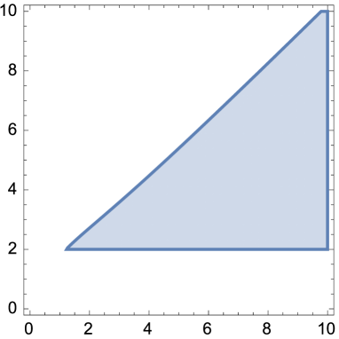
Figure 1: Region in a $(k_{1},k_{2})$-plane such that $R_{1}^{2}>0,\ R_{2}^{2}>0,\ z_{21}>0$ and $q[I_{1}]=0$ for $n_{1}=5$ $n_{2}=-4$, $l_{1}=l_{2}=1$.

IV.2 No CTCs

We demand that the domain of outer communication in the five-dimensional spacetime does not admits CTCs. This is achieved if the inequalities

$$g_{\theta\theta}>0,\qquad g_{\psi\psi}>0\,,\qquad g_{\psi\psi}g_{\phi\phi}-g_{\psi\phi}^{2}>0\,.$$ (72)

are satisfied on and outside all horizons. Explicitly, these conditions are replaced by

$$D_{1}: =K^{2}+HL>0\,,$$ (73)

$$D_{2}: =\frac{3}{4}K^{2}L^{2}-2K^{3}M-3HKLM+HL^{3}-H^{2}M^{2}>0\,,$$ (74)

$$D_{3}: =D_{2}r^{2}\sin^{2}\theta-\hat{\omega}_{\phi}^{2}>0\,.$$ (75)

It is a considerably troublesome problem to prove their positivity.

As seen in FIG. 2, for $n=2$, we have checked the absence of CTCs by seeing numerically the positivity of $D_{i}\ (i=1,2,3)$ and found that there appear no causal violations in the domain of outer communications. We can expect that for $n=2$, the inequalities (48) are sufficient to remove CTCs in the whole domain of outer communication. We also expect that even for $n>2$, (48) are sufficient to remove causal pathologies on and outside the horizon.

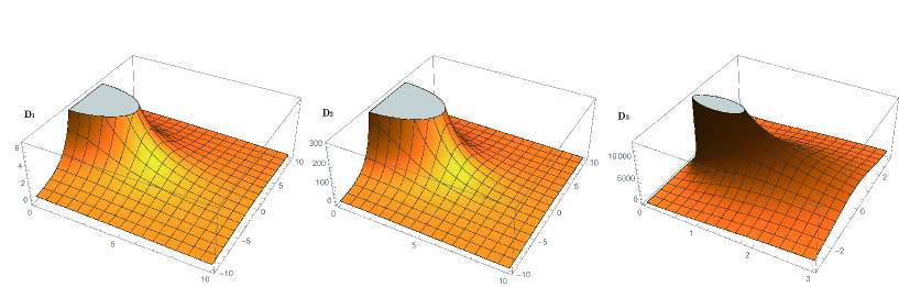
Figure 2: Plots of $D_{i}$’s against ($\rho=\sqrt{x^{2}+y^{2}},z$) for $n_{1}=2$ $n_{2}=-1$ , $z_{1}=0$, $z_{2}\simeq 0.0011$, $k_{1}=k_{2}=4$, $l_{1}=l_{2}=1$, $m_{1}=0$, $m_{2}=0.001$. No naked CTC appears.

IV.3 Critical surfaces

One of physically interesting features is that the harmonic function $H$ becomes negative around ${\bm{r}}={\bm{r}}_{i}$ ($i=1,\cdots,n$), which leads to the ($-,-,-,-$) signature of the Gibbons-Hawking base space. However, the signature of the five-dimensional spacetime metric remains Lorenzian because the function $f^{-1}H$ is positive. In this case, a so-called evanescent ergosurface appears Bena:2007kg at the places which $f=0$ corresponding to $H=0$.

At this surface, one must impose the regularity condition $K\neq 0$ when $H=0$ since if this does not hold, the spacetime could not become regular there. In other words, if there exist points $z=z_{c}$ on the axis such that

$$H=\sum_{i}\frac{n_{i}}{|z_{c}-z_{i}|}=0,\qquad K=\sum_{i}\frac{k_{i}}{|z_{c}-z_{i}|}=0,$$ (76)

these critical surfaces are singular, which leads to

$$\sum_{i\geq 2}\frac{n_{1}k_{i}-n_{i}k_{1}}{|z_{c}-z_{i}|}=0.$$ (77)

Hence, for instance, one of the sufficient conditions to avoid the singularities at critical surfaces is that for any $i$ $(i=1,\cdots,n)$, $n_{1}k_{i}-n_{i}k_{1}$ must have the same signs

$$n_{1}k_{i}-n_{i}k_{1}>0,\qquad{\rm or,}\qquad n_{1}k_{i}-n_{i}k_{1}<0.$$ (78)

For $n=2$, one of evanescent ergosurfaces exists at

$$z=\frac{n_{1}z_{2}+n_{2}z_{1}}{n_{1}+n_{2}}$$ (79)

for $z\in I_{+}$ when $n_{1}>0$ and $z\in I_{-}$ when $n_{1}<0$, whereas the other exists at

$$z=\frac{n_{1}z_{2}-n_{2}z_{1}}{n_{1}-n_{2}}$$ (80)

for $z\in I_{1}$.

V Summary

In this work, we have constructed an asymptotically flat and stationary multi-black lens solution as a supersymmetric solution in the bosonic sector of the five-dimensional minimal supergravity. We have shown that this solution describes mechanical equilibrium state of an arbitrary number of charged black lenses and the degenerate Killing horizons admit different lens space topologies $L(n_{i},1)=S^{3}/{\mathbb{Z}}_{n_{i}}\ (i=1,\cdots,n)$, where each $n_{i}$ takes non-zero different integers but must satisfy the constraint equation $\sum_{i=1}^{n}n_{i}=1$. This multi-black lens spacetime has a spatial symmetry of $U(1)\times U(1)$ because all horizons are alined on the $z$-axis in the Gibbons-Hawking space. Moreover, we have also computed the conserved charges including the (positive and BPS-saturating) mass, two angular momenta and the magnetic fluxes on the bubbles.

As for the supersymmetric black lens solution in obtained in Kunduri:2014kja ; Tomizawa:2016kjh , there exists no limit such that all the magnetic fluxes vanish. Therefore, one can consider that, at least, for the supersymmetric black lens with the single horizon of the topology $L(n,1)=S^{3}/{\mathbb{Z}}_{n}$ $(n=2,3,\cdots)$ in Kunduri:2014kja ; Tomizawa:2016kjh , the existence of the magnetic fluxes plays an essential role in supporting the horizon of the black lens. On the other hand, for the supersymmetric multi-black lenses obtained in this paper, it seems that the magnetic flux does not necessarily need to exist.

In this work, we have considered the supersymmetric solution subject to the constraint (28), which comes from the requirement that the topology of spatial infinity $r\to\infty$ should be $S^{3}$, when the spacetime asymptotically becomes flat. This constraint seems to impose a considerably strong restriction on the topologies of horizons. However, if one replaces the harmonic function $H$ in the Gibbons-Hawking base space with, for instance, another one

$$\sum_{i=1}^{n}\frac{n_{i}}{r_{i}}-\sum_{i=n+1}^{N}\frac{1}{r_{i}}\ \left(N:=\sum_{i=1}^{n}{n_{i}}-1\right)$$

and moreover, if at each point ${\bm{r}}={\bm{r}}_{i}\ (i=n+1,\cdots,N)$ where the harmonic function diverges, one demand regularity (this corresponds to the conditions $c_{2}=0$ in Tomizawa:2016kjh ) one no longer may need to impose the constraint (28). In this case, each horizon ${\bm{r}}={\bm{r}}_{i}\ (i=1,\cdots,n)$ can have an independent lens space topology of $L(n_{i},1)$.

References

• (1) F. R. Tangherlini, “Schwarzschild field in n dimensions and the dimensionality of space problem,” Nuovo Cim.  27, 636 (1963).
• (2) R. C. Myers and M. J. Perry, “Black Holes in Higher Dimensional Space-Times,” Annals Phys.  172, 304 (1986).
• (3) R. Emparan and H. S. Reall, “A Rotating black ring solution in five-dimensions,” Phys. Rev. Lett.  88, 101101 (2002) [hep-th/0110260].
• (4) A. A. Pomeransky and R. A. Sen’kov, “Black ring with two angular momenta,” hep-th/0612005.
• (5) R. Emparan and H. S. Reall, “Black Holes in Higher Dimensions,” Living Rev. Rel.  11 (2008) 6 [arXiv:0801.3471 [hep-th]].
• (6) J. P. Gauntlett, J. B. Gutowski, C. M. Hull, S. Pakis and H. S. Reall, “All supersymmetric solutions of minimal supergravity in five- dimensions,” Class. Quant. Grav.  20, 4587 (2003) [hep-th/0209114].
• (7) J. Bellorín, P. Meessen and T. Ortín, “All the supersymmetric solutions of $N=1$, $d=5$ ungauged supergravity,” JHEP 0701 (2007) 020 [hep-th/0610196].
• (8) J. B. Gutowski and W. Sabra, “General supersymmetric solutions of five-dimensional supergravity,” JHEP 0510 (2005) 039 [hep-th/0505185].
• (9) J. Bellorín and T. Ortín, “Characterization of all the supersymmetric solutions of gauged $N=1$, $d=5$ supergravity,” JHEP 0708 (2007) 096 [arXiv:0705.2567 [hep-th]].
• (10) J. P. Gauntlett, R. C. Myers and P. K. Townsend, “Black holes of D = 5 supergravity,” Class. Quant. Grav.  16, 1 (1999) [hep-th/9810204].
• (11) J. Grover, J. B. Gutowski and W. Sabra, “Null half-supersymmetric solutions in five-dimensional supergravity,” JHEP 0810 (2008) 103 [arXiv:0802.0231 [hep-th]].
• (12) J. B. Gutowski and W. A. Sabra, “Half-supersymmetric solutions in five-dimensional supergravity,” JHEP 0712 (2007) 025 [Erratum-ibid.  1004 (2010) 042] [arXiv:0706.3147 [hep-th]].
• (13) H. S. Reall, “Higher dimensional black holes and supersymmetry,” Phys. Rev. D 68, 024024 (2003) Erratum: [Phys. Rev. D 70, 089902 (2004)] [hep-th/0211290].
• (14) J. C. Breckenridge, R. C. Myers, A. W. Peet and C. Vafa, “D-branes and spinning black holes,” Phys. Lett. B 391, 93 (1997) [hep-th/9602065].
• (15) G. W. Gibbons and C. A. R. Herdeiro, “Supersymmetric rotating black holes and causality violation,” Class. Quant. Grav.  16, 3619 (1999) [hep-th/9906098].
• (16) H. Elvang, R. Emparan, D. Mateos and H. S. Reall, “A Supersymmetric black ring,” Phys. Rev. Lett.  93, 211302 (2004) [hep-th/0407065].
• (17) H. Elvang, R. Emparan, D. Mateos and H. S. Reall, “Supersymmetric black rings and three-charge supertubes,” Phys. Rev. D 71, 024033 (2005) [hep-th/0408120].
• (18) H. Elvang, R. Emparan and P. Figueras, “Non-supersymmetric black rings as thermally excited supertubes,” JHEP 0502 (2005) 031 [hep-th/0412130].
• (19) G. Compere, K. Copsey, S. de Buyl and R. B. Mann, “Solitons in Five Dimensional Minimal Supergravity: Local Charge, Exotic Ergoregions, and Violations of the BPS Bound,” JHEP 0912, 047 (2009) [arXiv:0909.3289 [hep-th]].
• (20) G. W. Gibbons and N. P. Warner, “Global structure of five-dimensional fuzzballs,” Class. Quant. Grav.  31, 025016 (2014) [arXiv:1305.0957 [hep-th]].
• (21) H. K. Kunduri and J. Lucietti, “Black hole non-uniqueness via spacetime topology in five dimensions,” JHEP 1410, 82 (2014) [arXiv:1407.8002 [hep-th]].
• (22) H. K. Kunduri and J. Lucietti, “The first law of soliton and black hole mechanics in five dimensions,” Class. Quant. Grav.  31, no. 3, 032001 (2014) [arXiv:1310.4810 [hep-th]].
• (23) B. E. Niehoff and H. S. Reall, “Evanescent ergosurfaces and ambipolar hyperkähler metrics,” JHEP 1604, 130 (2016) [arXiv:1601.01898 [hep-th]].
• (24) S. Tomizawa and S. Mizoguchi, “General Kaluza-Klein black holes with all six independent charges in five-dimensional minimal supergravity,” Phys. Rev. D 87 (2013) no.2, 024027 [arXiv:1210.6723 [hep-th]].
• (25) S. Mizoguchi and S. Tomizawa, “Flipped $SL(2,R)$ duality in five-dimensional supergravity,” Phys. Rev. D 86 (2012) 024022 [arXiv:1201.3063 [hep-th]].
• (26) S. Mizoguchi and S. Tomizawa, “New approach to solution generation using SL(2,R)-duality of a dimensionally reduced space in five-dimensional minimal supergravity and new black holes,” Phys. Rev. D 84 (2011) 104009 [arXiv:1106.3165 [hep-th]].
• (27) S. Tomizawa, Y. Yasui and Y. Morisawa, “Charged Rotating Kaluza-Klein Black Holes Generated by G2(2) Transformation,” Class. Quant. Grav.  26 (2009) 145006 [arXiv:0809.2001 [hep-th]].
• (28) S. Tomizawa and A. Ishibashi, “Charged Black Holes in a Rotating Gross-Perry-Sorkin Monopole Background,” Class. Quant. Grav.  25 (2008) 245007 [arXiv:0807.1564 [hep-th]].
• (29) K. Matsuno, H. Ishihara, T. Nakagawa and S. Tomizawa, “Rotating Kaluza-Klein Multi-Black Holes with Godel Parameter,” Phys. Rev. D 78 (2008) 064016 [arXiv:0806.3316 [hep-th]].
• (30) S. Tomizawa, “Multi-Black Rings on Eguchi-Hanson Space,” Class. Quant. Grav.  25 (2008) 145014 [arXiv:0802.0741 [hep-th]].
• (31) T. Nakagawa, H. Ishihara, K. Matsuno and S. Tomizawa, “Charged Rotating Kaluza-Klein Black Holes in Five Dimensions,” Phys. Rev. D 77 (2008) 044040 [arXiv:0801.0164 [hep-th]].
• (32) S. Tomizawa, H. Ishihara, M. Kimura and K. Matsuno, “Supersymmetric black rings on Eguchi-Hanson space,” Class. Quant. Grav.  24 (2007) 5609 [arXiv:0705.1098 [hep-th]].
• (33) H. Ishihara, M. Kimura, K. Matsuno and S. Tomizawa, “Black Holes on Eguchi-Hanson Space in Five-Dimensional Einstein-Maxwell Theory,” Phys. Rev. D 74 (2006) 047501 [hep-th/0607035].
• (34) H. Ishihara, M. Kimura, K. Matsuno and S. Tomizawa, “Kaluza-Klein Multi-Black Holes in Five-Dimensional Einstein-Maxwell Theory,” Class. Quant. Grav.  23 (2006) 6919 [hep-th/0605030].
• (35) H. Ishihara and K. Matsuno, “Kaluza-Klein black holes with squashed horizons,” Prog. Theor. Phys.  116 (2006) 417 [hep-th/0510094].
• (36) I. Bena and N. P. Warner, “One ring to rule them all … and in the darkness bind them?,” Adv. Theor. Math. Phys.  9, no. 5, 667 (2005) [hep-th/0408106].
• (37) I. Bena and N. P. Warner, “Black holes, black rings and their microstates,” Lect. Notes Phys.  755, 1 (2008) [hep-th/0701216].
• (38) I. Bena, S. Giusto, C. Ruef and N. P. Warner, “A (Running) Bolt for New Reasons,” JHEP 0911, 089 (2009) [arXiv:0909.2559 [hep-th]].
• (39) M. l. Cai and G. J. Galloway, “On the Topology and area of higher dimensional black holes,” Class. Quant. Grav.  18, 2707 (2001) [hep-th/0102149].
• (40) G. J. Galloway and R. Schoen, “A Generalization of Hawking’s black hole topology theorem to higher dimensions,” Commun. Math. Phys.  266, 571 (2006) [gr-qc/0509107].
• (41) S. Hollands and S. Yazadjiev, “Uniqueness theorem for 5-dimensional black holes with two axial Killing fields,” Commun. Math. Phys.  283, 749 (2008) [arXiv:0707.2775 [gr-qc]].
• (42) S. Hollands, J. Holland and A. Ishibashi, “Further restrictions on the topology of stationary black holes in five dimensions,” Annales Henri Poincare 12, 279 (2011) [arXiv:1002.0490 [gr-qc]].
• (43) J. Evslin, “Geometric Engineering 5d Black Holes with Rod Diagrams,” JHEP 0809, 004 (2008) [arXiv:0806.3389 [hep-th]].
• (44) Y. Chen and E. Teo, “A Rotating black lens solution in five dimensions”, Phys. Rev. D 78, 064062 (2008).
• (45) H. K. Kunduri and J. Lucietti,“Supersymmetric Black Holes with Lens-Space Topology”, Phys. Rev. Lett.  113, no. 21, 211101 (2014).
• (46) H. K. Kunduri and J. Lucietti, “Black lenses in string theory,” Phys. Rev. D 94 (2016) no.6, 064007 [arXiv:1605.01545 [hep-th]].
• (47) S. Tomizawa and M. Nozawa, “Supersymmetric black lenses in five dimensions,” Phys. Rev. D 94, no. 4, 044037 (2016).
• (48) S. D. Majumdar, “A class of exact solutions of Einstein’s field equations,” Phys. Rev.  72, 390 (1947).
• (49) A. Papapetrou, “Einstein’s theory of gravitation and flat space,” Proc. Roy. Irish Acad. (Sect. A) 52A, 11 (1948).
• (50) R. C. Myers, “Higher Dimensional Black Holes in Compactified Space-times,” Phys. Rev. D 35 (1987) 455.
• (51) D. L. Welch, “On the smoothness of the horizons of multi - black hole solutions,” Phys. Rev. D 52 (1995) 985 [hep-th/9502146].
• (52) G. N. Candlish and H. S. Reall, “On the smoothness of static multi-black hole solutions of higher-dimensional Einstein-Maxwell theory,” Class. Quant. Grav.  24 (2007) 6025 [arXiv:0707.4420 [gr-qc]].
• (53) G. N. Candlish, “On the smoothness of the multi-BMPV black hole spacetime,” Class. Quant. Grav.  27 (2010) 065005 [arXiv:0904.3885 [hep-th]].
• (54) J. B. Hartle and S. W. Hawking, “Solutions of the Einstein-Maxwell equations with many black holes,” Commun. Math. Phys.  26 (1972) 87.
• (55) I. Bena, P. Kraus and N. P. Warner, “Black rings in Taub-NUT,” Phys. Rev. D 72, 084019 (2005) [hep-th/0504142].