Minimax Optimal Estimators for Additive Scalar Functionals of Discrete Distributions

Abstract

In this paper, we consider estimators for an additive functional of $\phi$, which is defined as $\theta(P;\phi)=\sum_{i=1}^{k}\phi(p_{i})$, from $n$ i.i.d. random samples drawn from a discrete distribution $P=(p_{1},...,p_{k})$ with alphabet size $k$. We propose a minimax optimal estimator for the estimation problem of the additive functional. We reveal that the minimax optimal rate is characterized by the divergence speed of the fourth derivative of $\phi$ if the divergence speed is high. As a result, we show there is no consistent estimator if the divergence speed of the fourth derivative of $\phi$ is larger than $p^{-4}$. Furthermore, if the divergence speed of the fourth derivative of $\phi$ is $p^{4-\alpha}$ for $\alpha\in(0,1)$, the minimax optimal rate is obtained within a universal multiplicative constant as $\frac{k^{2}}{(n\ln n)^{2\alpha}}+\frac{k^{2-2\alpha}}{n}$.

1 Introduction

Let $P$ be a probability measure with alphabet size $k$, and $X$ be a discrete random variable drawn from $P$. Without loss of generality, we can assume that the domain of $P$ is $[k]$, where we denote $[m]=\{1,...,m\}$ for a positive integer $m$. We use a vector representation of $P$; $P=(p_{1},...,p_{k})$ where $p_{i}=P\{X=i\}$. Let $\phi$ be a mapping from $[0,1]$ to $\mathbb{R}^{+}$. Given a set of i.i.d. samples $S_{n}=\{X_{1},...,X_{n}\}$ from $P$, we deal with the problem of estimating an additive functional of $\phi$. The additive functional $\theta$ of $\phi$ is defined as

$$\theta(P;\phi)=\sum_{i=1}^{k}\phi(p_{i}).$$ (2)

We simplify this notation to $\theta(P;\phi)=\theta(P)$. Most entropy-like criteria can be formed in terms of $\theta$. For instance, when $\phi(p)=-p\ln p$, $\theta$ is Shannon entropy. For a positive real $\alpha$, letting $\phi(p)=p^{\alpha}$, $\ln(\theta(P))/(1-\alpha)$ becomes Rényi entropy. More generally, letting $\phi=f$ where $f$ is a concave function, $\theta$ becomes $f$-entropies (Akaike, 1998).

Techniques for the estimation of the entropy-like criteria have been considered in various fields, including physics (Lake and Moorman, 2011), neuroscience (Nemenman et al., 2004), and security (Gu et al., 2005). In machine learning, methods that involve entropy estimation were introduced for decision-trees (Quinlan, 1986), feature selection (Peng et al., 2005), and clustering (Dhillon et al., 2003). For example, the decision-tree learning algorithms, i.e., ID3, C4.5, and C5.0 construct a decision tree in which the criteria for the tree splitting are defined based on Shannon entropy (Quinlan, 1986). Similarly, information theoretic feature selection algorithms evaluate the relevance between the features and the target using the entropy (Peng et al., 2005).

The goal of this study is to derive the minimax optimal estimator of $\theta$ given a function $\phi$. For the precise definition of the minimax optimality, we introduce the minimax risk. A sufficient statistic of $P$ is a histogram $N=\lparen N_{1},...,N_{k}\rparen$, where $N_{j}=\sum_{i=1}^{n}{\boldsymbol{1}}_{\{X_{i}=j\}}$ and $N\sim\operatorname{{\rm Multinomial}}(n,P)$. The estimator of $\theta$ is defined as a function $\hat{\theta}:[n]^{k}\to\mathbb{R}$. Then, the quadratic minimax risk is defined as

$$R^{*}(n,k;\phi)=\inf_{\hat{\theta}}\sup_{P\in{\mathcal{M}}_{k}}\mathbf{E}\left[\left\lparen\hat{\theta}(N)-\theta(P)\right\rparen^{2}\right],$$ (3)

where ${\mathcal{M}}_{k}$ is the set of all probability measures on $[k]$, and the infimum is taken over all estimators $\hat{\theta}$. With this definition of the minimax risk, an estimator $\hat{\theta}$ is minimax (rate-)optimal if there exists a positive constant $C$ such that

$$\sup_{P\in{\mathcal{M}}_{k}}\mathbf{E}\left[\left\lparen\hat{\theta}(N)-\theta(P)\right\rparen^{2}\right]\leq CR^{*}(n,k;\phi).$$ (4)

A natural estimator of $\theta$ is the plugin or the maximum likelihood estimator, in which the estimated value is obtained by substituting the empirical mean of the probabilities $P$ into $\theta$. However, the estimator has a large bias for large $k$. Indeed, the plugin estimators for $\phi(p)=-p\ln p$ and $\phi(p)=p^{\alpha}$ have been shown to be suboptimal in the large-$k$ regime in recent studies (Wu and Yang, 2016; Jiao et al., 2015; Acharya et al., 2015).

Recent studies investigated the minimax optimal estimators for $\phi(p)=-p\ln p$ and $\phi(p)=p^{\alpha}$ in the large-$k$ regime (Wu and Yang, 2016; Jiao et al., 2015; Acharya et al., 2015). However, the results of these studies were only derived for these $\phi$. Jiao et al. (2015) suggested that the estimator is easily extendable to the general additive functional, although they did not prove the minimax optimality.

In this paper, we propose a minimax optimal estimator for the estimation problem of the additive functional $\theta$ for general $\phi$ under certain conditions on the smoothness. Our estimator achieves the minimax optimal rate even in the large-$k$ regime for $\phi\in C^{4}[0,1]$ such that $\left\lvert\phi^{(4)}(p)\right\rvert$ is finite for $p\in(0,1]$, where $C^{4}[0,1]$ denotes a class of four times differentiable functions from $[0,1]$ to $\mathbb{R}$. For such $\phi$, we reveal a property of $\phi$ which can substantially influence the minimax optimal rate.

Related work. The simplest way to estimate $\theta$ is to use the so-called plugin estimator or the maximum likelihood estimator, in which the empirical probabilities are substituted into $\theta$ as $P$. Letting $\tilde{P}=(\hat{p}_{1},...,\hat{p}_{k})$ and $\hat{p}_{i}=N_{i}/n$, the plugin estimator is defined as

$$\theta_{\rm plugin}(N)=\theta(\tilde{P}).$$ (5)

The plugin estimator is asymptotically consistent under weak assumptions for fixed $k$ (Antos and Kontoyiannis, 2001). However, this is not true for the large-$k$ regime. Indeed, Jiao et al. (2015) and Wu and Yang (2016) derived a lower bound for the quadratic risk for the plugin estimator of $\phi(p)=p\ln(1/p)$ and $\phi(p)=p^{\alpha}$. In the case of Shannon entropy, the lower bound is given as

$$\sup_{P\in{\mathcal{M}}_{k}}\mathbf{E}\left[\left\lparen\theta_{\rm plugin}(N)-\theta(P)\right\rparen^{2}\right]\geq C\left\lparen\frac{k^{2}}{n^{2}}+\frac{\ln^{2}k}{n}\right\rparen,$$ (6)

where $C$ denotes a universal constant. The first term $k^{2}/n^{2}$ comes from the bias and it indicates that if $k$ grows linearly with respect to $n$, the plugin estimator becomes inconsistent. This means the plugin estimator is suboptimal in the large-$k$ regime. Bias-correction methods, such as (Miller, 1955; Grassberger, 1988; Zahl, 1977), can be applied to the plugin estimator of $\phi(p)=-p\ln p$ to reduce the bias whereas these bias-corrected estimators are still suboptimal. The estimators based on Bayesian approaches in (Schürmann and Grassberger, 1996; Schober, 2013; Holste et al., 1998) are also suboptimal (Han et al., 2015).

Many researchers have studied estimators that can consistently estimate the additive functional with sublinear samples with respect to the alphabet size $k$ to derive the optimal estimator in the large-$k$ regime. The existence of consistent estimators even with sublinear samples were first revealed in Paninski (2004), but an explicit estimator was not provided. Valiant and Valiant (2011a) introduced an estimator based on linear programming that consistently estimates $\phi(p)=-p\ln p$ with sublinear samples. However, the estimator of (Valiant and Valiant, 2011a) has not been shown to achieve the minimax rate even in a more detailed analysis in (Valiant and Valiant, 2011b). Recently, Acharya et al. (2015) showed that the bias-corrected estimator of Rényi entropy achieves the minimax optimal rate in regard to the sample complexity if $\alpha>1$ and $\alpha\in\mathbb{N}$, but they did not show the minimax optimality for other $\alpha$. Jiao et al. (2015) introduced a minimax optimal estimator for $\phi(p)=-p\ln p$ for any $\alpha\in(0,3/2)$ in the large-$k$ regime. Wu and Yang (2015) derived a minimax optimal estimator for $\phi(p)={\boldsymbol{1}}_{p>0}$. For $\phi(p)=-p\ln p$, Jiao et al. (2015); Wu and Yang (2016) independently introduced the minimax optimal estimators in the large-$k$ regime. In the case of Shannon entropy, the optimal rate was obtained as

$$\frac{k^{2}}{(n\ln n)^{2}}+\frac{\ln^{2}k}{n}.$$ (7)

The first term indicates that the introduced estimator can consistently estimate Shannon entropy if $n\geq Ck/\ln k$.

The estimators introduced by Wu and Yang (2016); Jiao et al. (2015); Acharya et al. (2015) are composed of two estimators: the bias-corrected plugin estimator and the best polynomial estimator. The bias-corrected plugin estimator is composed of the sum of the plugin estimator and a bias-correction term which offsets the second-order approximation of the bias as in (Miller, 1955). The best polynomial estimator is an unbiased estimator of the polynomial that best approximates $\phi$ in terms of the uniform error. Specifically, the best approximation for the polynomial of $\phi$ in an interval $I\subseteq[0,1]$ is the polynomial $g$ that minimizes $\sup_{x\in I}\left\lvert\phi(x)-g(x)\right\rvert$. Jiao et al. (2015) suggested that this estimator can be extended for the general additive functional $\theta$. However, the minimax optimality of the estimator was only proved for specific cases of $\phi$, including $\phi(p)=-p\ln p$ and $\phi(p)=p^{\alpha}$. Thus, to prove the minimax optimality for other $\phi$, we need to individually analyze the minimax optimality for specific $\phi$. Here, we aim to clarify which property of $\phi$ substantially influences the minimax optimal rate when estimating the additive functional.

Besides, the optimal estimators for divergences with large alphabet size have been investigated in (Bu et al., 2016; Han et al., 2016; Jiao et al., 2016). The estimation problems of divergences are much complicated than the additive function, while the similar techniques were applied to derive the minimax optimality.

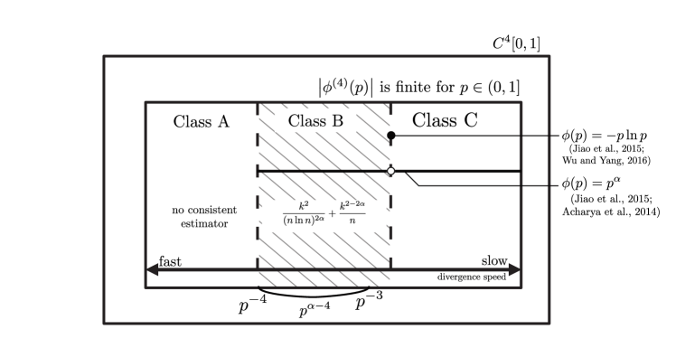
Figure 1: Relationship between the divergence speed of the fourth derivative of $\phi$ and the minimax optimality of the estimation problem of $\theta(P;\phi)$.

Our contributions. In this paper, we propose the minimax optimal estimator for $\theta(P;\phi)$. We reveal that the divergence speed of the fourth derivative of $\phi$ plays an important role in characterizing the minimax optimal rate. Informally, for $\beta>0$, the meaning of “the divergence speed of a function $f(p)$ is $p^{-\beta}$” is that $\left\lvert f(p)\right\rvert$ goes to infinity at the same speed as $p^{-\beta}$ when $p$ approaches $0$. When the divergence speed of the fourth derivative of $\phi(p)$ is $p^{-\beta}$, the fourth derivative of $\phi$ diverges faster as $\beta$ increases.

Our results are summarized in Figure 1. Figure 1 illustrates the relationship between the divergence speed of the fourth derivative of $\phi$ and the minimax optimality of the estimation problem of $\theta(P;\phi)$. In Figure 1, the outermost rectangle represents the space of the four times continuous differentiable functions $C^{4}[0,1]$. The innermost rectangle denotes the subset class of $C^{4}[0,1]$ such that the absolute value of its fourth derivative $\left\lvert\phi^{(4)}(p)\right\rvert$ is finite for any $p\in(0,1]$. In this subclass of $\phi$, the horizontal direction represents the divergence speed of the fourth derivative of $\phi$, in which a faster $\phi$ is on the left-hand side and a slower $\phi$ is on the right-hand side. The $\phi$ with an explicit form and divergence speed is denoted by a point in the rectangle. For example, the black circle denotes $\phi(p)=-p\ln p$ where the divergence speed of the fourth derivative of this $\phi$ is $p^{-3}$. Class B denotes a set of any function $\phi$ such that the divergence speed of the fourth derivative is $p^{\alpha-4}$ where $\alpha\in(0,1)$. As already discussed, existing methods have achieved minimax optimality in the large-$k$ regime for specific $\phi$, including $\phi(p)=-p\ln p$ (black circle in Figure 1) and $\phi(p)=p^{\alpha}$ (middle line in Figure 1 where the white circle denotes that there is no $\alpha>0$ such that the divergence speed is $p^{-3}$).

We investigate the minimax optimality of the estimation problem of $\theta$ for $\phi$ in Class A and Class B. Class A is a class of $\phi$ such that the divergence speed of the fourth derivative is faster than $p^{-4}$. Class B is a class of $\phi$ such that the divergence speed of the fourth derivative is $p^{\alpha-4}$ where $\alpha\in(0,1)$. In Class A, we show that we cannot construct a consistent estimator of $\theta$ for any $\phi$ in Class A (the leftmost hatched area in Figure 1, Proposition 1). In other words, the minimax optimal rate is larger than constant order if the divergence speed of the fourth derivative is faster than $p^{-4}$. Thus, there is no need to derive the minimax optimal estimator in Class A.

Also, we derive the minimax optimal estimator for any $\phi$ in Class B (the middle hatched area in Figure 1, Theorem 1). For example, $\phi(p)=p^{\alpha}$ (Réyni entropy case), $\phi(p)=\cos(cp)p^{\alpha}$, and $\phi(p)=e^{cp}p^{\alpha}$ for $\alpha\in(0,1)$ include the coverage of our estimator, where $c$ is a universal constant. Intuitively, since the large derivative makes the estimation problem $\theta$ more difficult, the minimax rate decreases if the derivative of $\phi$ diverges faster. Our minimax optimal rate reflects this behavior. For $\phi$ in Class B, the minimax optimal rate is obtained as

$$\frac{k^{2}}{(n\ln n)^{2\alpha}}+\frac{k^{2-2\alpha}}{n},$$ (8)

where $k\gtrsim\ln^{\frac{4}{3}}n$ if $\alpha\in(0,1/2]$. We can clearly see that this rate decreases for larger $\alpha$, i.e., a slower divergence speed.

Currently, the minimax optimality of $\phi$ in Class C is an open problem. However, we provide a notable discussion in Section 3.

2 Preliminaries

Notations. We now introduce some additional notations. For any positive real sequences $\{a_{n}\}$ and $\{b_{n}\}$, $a_{n}\gtrsim b_{n}$ denotes that there exists a positive constant $c$ such that $a_{n}\geq cb_{n}$. Similarly, $a_{n}\lesssim b_{n}$ denotes that there exists a positive constant $c$ such that $a_{n}\leq cb_{n}$. Furthermore, $a_{n}\asymp b_{n}$ implies $a_{n}\gtrsim b_{n}$ and $a_{n}\lesssim b_{n}$. For an event $\mathcal{E}$, we denote its complement by $\mathcal{E}^{c}$. For two real numbers $a$ and $b$, $a\lor b=\max\{a,b\}$ and $a\land b=\min\{a,b\}$. For a function $\phi:\mathbb{R}\to\mathbb{R}$, we denote its $i$-th derivative as $\phi^{(i)}$.

Poisson sampling. We employ the Poisson sampling technique to derive upper and lower bounds for the minimax risk. The Poisson sampling technique models the samples as independent Poisson distributions, while the original samples follow a multinomial distribution. Specifically, the sufficient statistic for $P$ in the Poisson sampling is a histogram $\tilde{N}=\lparen\tilde{N}_{i},...,\tilde{N}_{k}\rparen$, where $\tilde{N}_{1},...,\tilde{N}_{k}$ are independent random variables such that $\tilde{N}_{i}\sim\operatorname{{\rm Poi}}(np_{i})$. The minimax risk for Poisson sampling is defined as follows:

$$\tilde{R}^{*}(n,k;\phi)=\inf_{\{\hat{\theta}\}}\sup_{P\in{\mathcal{M}}_{k}}\mathbf{E}\left[\left\lparen\hat{\theta}(\tilde{N})-\theta(P)\right\rparen^{2}\right].$$ (9)

The minimax risk of Poisson sampling well approximates that of the multinomial distribution. Indeed, Jiao et al. (2015) presented the following lemma.

Lemma 1 (Jiao et al. (2015)).

The minimax risk under the Poisson model and the multinomial model are related via the following inequalities:

$$\tilde{R}^{*}(2n,k;\phi)-\sup_{P\in{\mathcal{M}}_{k}}\left\lvert\theta(P)\right\rvert e^{-n/4}\leq R^{*}(n,k;\phi)\leq 2\tilde{R}^{*}(n/2,k;\phi).$$ (10)

Lemma 1 states $R^{*}(n,k;\phi)\asymp\tilde{R}^{*}(n,k;\phi)$, and thus we can derive the minimax rate of the multinomial distribution from that of the Poisson sampling.

Best polynomial approximation. Acharya et al. (2015); Wu and Yang (2016); Jiao et al. (2015) presented a technique of the best polynomial approximation for deriving the minimax optimal estimators and their lower bounds for the risk. Let ${\mathcal{P}}_{L}$ be the set of polynomials of degree $L$. Given a function $\phi$, a polynomial $p$, and an interval $I\subseteq[0,1]$, the uniform error between $\phi$ and $p$ on $I$ is defined as

$$\sup_{x\in I}\left\lvert\phi(x)-p(x)\right\rvert.$$ (11)

The best polynomial approximation of $\phi$ by a degree-$L$ polynomial with a uniform error is achieved by the polynomial $p\in{\mathcal{P}}_{L}$ that minimizes Eq 11. The error of the best polynomial approximation is defined as

$$E_{L}\left\lparen\phi,I\right\rparen=\inf_{p\in{\mathcal{P}}_{L}}\sup_{x\in I}\left\lvert\phi(x)-p(x)\right\rvert.$$ (12)

The error rate with respect to the degree $L$ has been studied since the 1960s (Timan et al., 1965; Petrushev and Popov, 2011; Ditzian and Totik, 2012; Achieser, 2013). The polynomial that achieves the best polynomial approximation can be obtained, for instance, by the Remez algorithm (Remez, 1934) if $I$ is bounded.

3 Main results

Suppose $\phi$ is four times continuously differentiable on $(0,1]$. We reveal that the divergence speed of the fourth derivative of $\phi$ plays an important role for the minimax optimality of the estimation problem of the additive functional. Formally, the divergence speed is defined as follows.

Definition 1 (divergence speed).

For an integer $m\geq 1$, let $\phi$ be an $m$ times continuously differentiable function on $(0,1]$. For $\beta>0$, the divergence speed of the $m$th derivative of $\phi$ is $p^{-\beta}$ if there exist finite constants $W>0$, $c_{m}$, and $c^{\prime}_{m}$ such that for all $p\in(0,1]$

$$\left\lvert\phi^{(m)}(p)\right\rvert\leq\beta_{m-1}Wp^{-\beta}+c_{m},~{}{\rm and}~{}\left\lvert\phi^{(m)}(p)\right\rvert\geq\beta_{m-1}Wp^{-\beta}+c^{\prime}_{m},$$ (13)

where $\beta_{m}=\prod_{i=1}^{m}(i-m+\beta)$.

A larger $\beta$ implies faster divergence. We analyze the minimax optimality for two cases: the divergence speed of the fourth derivative of $\phi$ is i) larger than $p^{-4}$ (Class A), and ii) $p^{\alpha-4}$ (Class B), for $\alpha\in(0,1)$.

Minimax optimality for Class A. We now demonstrate that we cannot construct a consistent estimator for any $n$ and $k\geq 3$ if the divergence speed of $\phi$ is larger than $p^{-4}$.

Proposition 1.

Let $\phi$ be a continuously differentiable function on $(0,1]$. If there exists finite constants $W>0$ and $c^{\prime}_{1}$ such that for $p\in(0,1]$

$$\left\lvert\phi^{(1)}(p)\right\rvert\geq Wp^{-1}+c^{\prime}_{1},$$ (14)

then there is no consistent estimator, i.e., $R^{*}(n,k;\phi)\gtrsim 1$.

The proof of Proposition 1 is given in Appendix D. From Lemma 15, the divergence speed of the first derivative is $p^{-1}$ if that of the fourth derivative is $p^{-4}$. Thus, if the divergence speed of $\phi$ is greater than $p^{-4}$, we cannot construct an estimator that consistently estimates $\theta$ for any probability measure $P\in{\mathcal{M}}_{k}$. Consequently, there is no need to derive the minimax optimal estimator in this case.

Minimax optimality for Class B. We derive the minimax optimal rate for $\phi$ in which the divergence speed of its fourth derivative is $p^{\alpha-4}$ for $\alpha\in(0,1)$. Thus, we make the following assumption.

Assumption 1.

Suppose $\phi$ is four times continuously differentiable on $(0,1]$. For $\alpha\in(0,1)$, the divergence speed of the fourth derivative of $\phi$ is $p^{\alpha-4}$.

Note that a set of $\phi$ satisfying Assumption 1 is Class B depicted in Figure 1. The divergence speed increases as $\alpha$ decreases. Under Assumption 1, we derive the minimax optimal estimator of which the minimax rate is given by the following theorems.

Theorem 1.

Under Assumption 1 with $\alpha\in(0,1/2]$, if $n\gtrsim\frac{k^{1/\alpha}}{\ln k}$ and $k\gtrsim\ln^{\frac{4}{3}}n$,

$$R^{*}(n,k;\phi)\asymp\frac{k^{2}}{(n\ln n)^{2\alpha}}.$$ (15)

Otherwise, there is no consistent estimator, i.e., $R^{*}(n,k;\phi)\gtrsim 1$.

Theorem 2.

Under Assumption 1 with $\alpha\in(1/2,1)$, if $n\gtrsim\frac{k^{1/\alpha}}{\ln k}$

$$R^{*}(n,k;\phi)\asymp\frac{k^{2}}{(n\ln n)^{2\alpha}}+\frac{k^{2-2\alpha}}{n}.$$ (16)

Otherwise, there is no consistent estimator, i.e., $R^{*}(n,k;\phi)\gtrsim 1$.

Theorems 1 and 2 are proved by combining the results in Sections 6 and 7. The minimax optimal rate in Theorems 1 and 2 are characterized by the parameter for the divergence speed $\alpha$ from Assumption 1. From Theorems 1 and 2, we can conclude that the minimax optimal rate decreases as the divergence speed increases.

The explicit estimator that achieves the optimal minimax rate shown in Theorems 1 and 2 are described in the next section.

Remark 1.

Assumption 1 covers $\phi(p)=p^{\alpha}$ for $\alpha\in(0,1)$, but does not for all existing works. For $\phi(p)=-p\ln(p)$ and $\phi(p)=p^{\alpha}$ with $\alpha\geq 1$, the divergence speed of these $\phi$ is lower than $p^{\alpha-4}$ for $\alpha\in(0,1)$. Indeed, the divergence speed of $\phi(p)=-p\ln(p)$ and $\phi(p)=p^{\alpha}$ for $\alpha\geq 1$ are $p^{-3}$ and $p^{\alpha-4}$, respectively. We can expect that the corresponding minimax rate is characterized by the divergence speed even if the divergence speed is lower than $p^{\alpha-4}$ for $\alpha\in(0,1)$. The analysis of the minimax rate for lower divergence speeds remains an open problem.

4 Estimator for $\theta$

In this section, we describe our estimator for $\theta$ in detail. Our estimator is composed of the bias-corrected plugin estimator and the best polynomial estimator. We first describe the overall estimation procedure on the supposition that the bias-corrected plugin estimator and the best polynomial estimator are black boxes. Then, we describe the bias-corrected plugin estimator and the best polynomial estimator in detail.

For simplicity, we assume the samples are drawn from the Poisson sampling model, where we first draw $n^{\prime}\sim\operatorname{{\rm Poi}}(2n)$, and then draw $n^{\prime}$ i.i.d. samples $S_{n^{\prime}}=\{X_{1},...,X_{n^{\prime}}\}$. Given the samples $S_{n^{\prime}}$, we first partition the samples into two sets. We use one set of the samples to determine whether the bias-corrected plugin estimator or the best polynomial estimator should be employed, and the other set to estimate $\theta$. Let $\{B_{i}\}_{i=1}^{n^{\prime}}$ be i.i.d. random variables drawn from the Bernoulli distribution with parameter $1/2$, i.e., ${\mathbb{P}}\{B_{i}=0\}={\mathbb{P}}\{B_{i}=1\}=1/2$ for $i=1,...,n^{\prime}$. We partition $(X_{1},...,X_{n^{\prime}})$ according to $(B_{1},...,B_{n^{\prime}})$, and construct the histograms $\tilde{N}$ and $\tilde{N}^{\prime}$, which are defined as

$$\tilde{N}_{i}=\sum_{j=1}^{n^{\prime}}{\boldsymbol{1}}_{X_{j}=i}{\boldsymbol{1}}_{B_{j}=0},\quad\tilde{N}^{\prime}_{i}=\sum_{j=1}^{n^{\prime}}{\boldsymbol{1}}_{X_{j}=i}{\boldsymbol{1}}_{B_{j}=1},~{}{\rm for}~{}i\in[n^{\prime}].$$ (17)

Then, $\tilde{N}$ and $\tilde{N}^{\prime}$ are independent histograms, and $\tilde{N}_{i},\tilde{N}^{\prime}_{i}\sim\operatorname{{\rm Poi}}(np_{i})$.

Given $\tilde{N}^{\prime}$, we determine whether the bias-corrected plugin estimator or the best polynomial estimator should be employed for each alphabet. Let $\Delta_{n,k}$ be a threshold depending on $n$ and $k$ to determine which estimator is employed, which will be specified as in Theorem 5 on Theorem 5. We apply the best polynomial estimator if $\tilde{N}^{\prime}_{i}<2\Delta_{n,k}$, and otherwise, i.e., $\tilde{N}^{\prime}_{i}\geq 2\Delta_{n,k}$, we apply the bias-corrected plugin estimator. Let $\phi_{\rm poly}$ and $\phi_{\rm plugin}$ be the best polynomial estimator and the bias-corrected plugin estimator for $\phi$, respectively. Then, the estimator of $\theta$ is written as

$$\tilde{\theta}(\tilde{N})=\sum_{i=1}^{k}\left\lparen{\boldsymbol{1}}_{\tilde{N}^{\prime}_{i}\geq 2\Delta_{n,k}}\phi_{\rm plugin}(\tilde{N}_{i})+{\boldsymbol{1}}_{\tilde{N}^{\prime}_{i}<2\Delta_{n,k}}\phi_{\rm poly}(\tilde{N}_{i})\right\rparen.$$ (18)

Finally, we truncate $\tilde{\theta}$ so that the final estimate is not outside of the domain of $\theta$.

$$\hat{\theta}(\tilde{N})= (\tilde{\theta}(\tilde{N})\land\theta_{\rm sup})\lor\theta_{\rm inf},$$ (19)

where $\theta_{\rm inf}=\inf_{P\in{\mathcal{M}}_{k}}\theta(P)$ and $\theta_{\rm sup}=\sup_{P\in{\mathcal{M}}_{k}}\theta(P)$. Next, we describe the details of the best polynomial estimator $\phi_{\rm poly}$ and the bias-corrected plugin estimator $\phi_{\rm plugin}$.

Best polynomial estimator. The best polynomial estimator is an unbiased estimator of the polynomial that provides the best approximation of $\phi$. Let $\{a_{m}\}_{m=0}^{L}$ be coefficients of the polynomial that achieves the best approximation of $\phi$ by a degree-$L$ polynomial with range $I=[0,\frac{4\Delta_{n,k}}{n}]$, where $L$ is as specified in Theorem 5 on Theorem 5. Then, the approximation of $\phi$ by the polynomial at point $p_{i}$ is written as

$$\phi_{L}(p_{i})= \sum_{m=0}^{L}a_{m}p_{i}^{m}.$$ (20)

From Eq 20, an unbiased estimator of $\phi_{L}$ can be derived from an unbiased estimator of $p_{i}^{m}$. For the random variable $\tilde{N}_{i}$ drawn from the Poisson distribution with mean parameter $np_{i}$, the expectation of the $m$th factorial moment $(\tilde{N}_{i})_{m}=\tfrac{\tilde{N}_{i}!}{(\tilde{N}_{i}-m)!}$ becomes $(np_{i})^{m}$. Thus, $\frac{(\tilde{N}_{i})_{m}}{n^{m}}$ is an unbiased estimator of $p_{i}^{m}$. Substituting this into Eq 20 gives the unbiased estimator of $\phi_{L}(p_{i})$ as

$$\bar{\phi}_{\rm poly}(\tilde{N}_{i})=\sum_{m=0}^{L}\frac{a_{m}}{n^{j}}(\tilde{N}_{i})_{m}.$$ (21)

Next, we truncate $\bar{\phi}_{\rm poly}$ so that it is not outside of the domain of $\phi(p)$. Let $\phi_{{\rm inf},\frac{\Delta_{n,k}}{n}}=\inf_{p\in[0,\frac{\Delta_{n,k}}{n}]}\phi(p)$ and $\phi_{{\rm sup},\frac{\Delta_{n,k}}{n}}=\sup_{p\in[0,\frac{\Delta_{n,k}}{n}]}\phi(p)$. Then, the best polynomial estimator is defined as

$$\phi_{\rm poly}(\tilde{N}_{i})=(\bar{\phi}_{\rm poly}(\tilde{N}_{i})\land\phi_{{\rm sup},\frac{\Delta_{n,k}}{n}})\lor\phi_{{\rm inf},\frac{\Delta_{n,k}}{n}}.$$ (22)

Bias-corrected plugin estimator. In the bias-corrected plugin estimator, we apply the bias correction of (Miller, 1955). Applying the second-order Taylor expansion to the bias of the plugin estimator gives

$$\mathbf{E}\left[\phi\left\lparen\frac{\tilde{N}_{i}}{n}\right\rparen-\phi(p_{i})\right]\approx \mathbf{E}\left[\phi^{(1)}(p_{i})\left\lparen\frac{\tilde{N}_{i}}{n}-p_{i}\right\rparen+\frac{\phi^{(2)}(p_{i})}{2}\left\lparen\frac{\tilde{N}_{i}}{n}-p_{i}\right\rparen^{2}\right]$$ (23)

$$= \frac{p_{i}\phi^{(2)}(p_{i})}{2n}.$$ (24)

Thus, we include $-\frac{\tilde{N}_{i}\phi^{(2)}(\tilde{N}_{i}/n)}{2n^{2}}$ as a bias-correction term in the plugin estimator $\phi(\tilde{N}_{i}/n)$, which offsets the second-order approximation of the bias. However, we do not directly apply the bias-corrected plugin estimator to estimate $\phi(p_{i})$ for two reasons. First, the derivative of $\phi$ is large near $0$, which results in a large bias, and second, $\phi(p)$ for $p>1$ is undefined even though $\tilde{N}_{i}/n$ can exceed $1$. Thus, we apply the bias-corrected plugin estimator to the function $\bar{\phi}_{\frac{\Delta_{n,k}}{n}}$ defined below instead of $\phi$. Define

$$H_{L}(p;\phi,a,b)$$ (25)

$$= \phi(a)+\sum_{m=1}^{L}\frac{\phi^{(m)}(a)}{m!}(p-a)^{m}(p-b)^{L+1}\sum_{\ell=0}^{L-m}\frac{(-1)^{\ell}(L+\ell)!}{\ell!L!}(a-b)^{-L-1-\ell}(p-a)^{\ell}$$ (26)

$$= \phi(a)+\sum_{m=1}^{L}\frac{\phi^{(m)}(a)}{m!}(p-a)^{m}\sum_{\ell=0}^{L-m}\frac{L+1}{L+\ell+1}\operatorname{{\rm B}}_{\ell,L+\ell+1}\left\lparen\frac{p-a}{b-a}\right\rparen,$$ (27)

where $\operatorname{{\rm B}}_{\nu,n}(x)=\binom{n}{\nu}x^{\nu}(1-x)^{n-\nu}$ denotes the Bernstein basis polynomial. Then, $H_{L}(p;\phi,a,b)$ denotes a function that interpolates between $\phi(a)$ and $\phi(b)$ using Hermite interpolation. From generalized Hermite interpolation (Spitzbart, 1960), $H_{L}^{(i)}(a;\phi,a,b)=\phi^{(i)}(a)$ for $i=0,...,L$ and $H_{L}^{(i)}(b;\phi,a,b)=0$ for $i=1,...,L$. The function $\bar{\phi}_{\frac{\Delta_{n,k}}{n}}$ is defined as

$$\bar{\phi}_{\frac{\Delta_{n,k}}{n}}(p)=\begin{dcases}H_{4}\left\lparen\frac{\Delta_{n,k}}{2n};\phi,\frac{\Delta_{n,k}}{n},\frac{\Delta_{n,k}}{2n}\right\rparen&~{}{\rm if}~{}p\leq\frac{\Delta_{n,k}}{2n},\\ H_{4}\left\lparen p;\phi,\frac{\Delta_{n,k}}{n},\frac{\Delta_{n,k}}{2n}\right\rparen&~{}{\rm if}~{}\frac{\Delta_{n,k}}{2n}<p<\frac{\Delta_{n,k}}{n},\\ H_{4}\left\lparen p;\phi,1,2\right\rparen&~{}{\rm if}~{}1<p<2,\\ H_{4}\left\lparen 2;\phi,1,2\right\rparen&~{}{\rm if}~{}p\geq 2,\\ \phi(p)&~{}{\rm otherwise}~{}.\end{dcases}$$ (28)

From this definition, $\bar{\phi}_{\frac{\Delta_{n,k}}{n}}=\phi$ if $p\in[\frac{\Delta_{n,k}}{n},1]$. From Hermite interpolation, the function $\bar{\phi}_{\frac{\Delta_{n,k}}{n}}$ is four times differentiable on $\mathbb{R}_{+}$ and $\bar{\phi}_{\frac{\Delta_{n,k}}{n}}^{(1)}(p)=...=\bar{\phi}_{\frac{\Delta_{n,k}}{n}}^{(4)}(p)=0$ for $p\leq\frac{\Delta_{n,k}}{2n}$ and $p\geq 2$. By introducing $\bar{\phi}_{\frac{\Delta_{n,k}}{n}}$, we can bound the fourth derivative of $\bar{\phi}_{\frac{\Delta_{n,k}}{n}}$ using $\Delta_{n,k}$, and this enables us to control the bias with the threshold parameter $\Delta_{n,k}$. Using $\bar{\phi}_{\frac{\Delta_{n,k}}{n}}$ instead of $\phi$ yields the bias-corrected plugin estimator

$$\phi_{\rm plugin}(\tilde{N}_{i})=\bar{\phi}_{\frac{\Delta_{n,k}}{n}}\left\lparen\frac{\bar{N}_{i}}{n}\right\rparen-\frac{\tilde{N}_{i}}{2n^{2}}\bar{\phi}_{\frac{\Delta_{n,k}}{n}}^{(2)}\left\lparen\frac{\bar{N}_{i}}{n}\right\rparen.$$ (29)

5 Remark about Differentiability for Analysis

Why is the minimax rate characterized by the divergence speed of the fourth derivative? Indeed, most of the results can be obtained on a weaker assumption compared to Assumption 1 regarding differentiability, which is formally defined as follows.

Assumption 2.

Suppose $\phi$ is two times continuously differentiable on $(0,1]$. For $\alpha\in(0,1)$, the divergence speed of the second derivative of $\phi$ is $p^{\alpha-2}$.

Assumption 2 only requires two times continuous differentiability, whereas Assumption 1 requires four times. Only the analysis of the bias-corrected plugin estimator requires Assumption 1 to achieve the minimax rate due to the bias-correction term in Eq 29. The bias-correction term is formed as the plugin estimator of the second derivative of $\phi$, and its convergence rate is highly dependent on the smoothness of the second derivative. The smoothness of the second derivative of $\phi$ is characterized by the fourth derivative of $\phi$, and thus Assumption 1 is required to derive the error bound of the bias-corrected plugin estimator. Another bias-correction method might weaken the assumption as in Assumption 2.

6 Analysis of Lower Bound

In this section, we derive a lower bound for the minimax rate of $\theta$. Under Assumption 2, we can derive the lower bound of the minimax risk as in the following theorem.

Theorem 3.

Under Assumption 2, for $k\geq 3$, we have

$$R^{*}(n,k;\phi)\gtrsim\frac{k^{2-2\alpha}}{n}.$$ (30)

The lower bound is obtained by applying Le Cam’s two-point method (see (Tsybakov, 2009)). The details of the proof of Theorem 3 can be found in Appendix B. Next, we derive another lower bound for the minimax rate.

Theorem 4.

Under Assumption 2, if $n\gtrsim\frac{k^{1/\alpha}}{\ln k}$, we have

$$R^{*}(n,k;\phi)\gtrsim\frac{k^{2}}{(n\ln n)^{2\alpha}},$$ (31)

where we need $k\gtrsim\ln^{\frac{4}{3}}n$ if $\alpha\in(0,1/2]$.

The proof is accomplished in the same manner as (Wu and Yang, 2016, Proposition 3). The details of the proof of Theorem 4 are also found in Appendix B. Combining Theorems 3 and 4, we get the lower bounds in Theorems 1 and 2 as $R^{*}(n,k;\phi)\gtrsim\frac{k^{2}}{(n\ln n)^{2\alpha}}\lor\frac{k^{2-2\alpha}}{n}\gtrsim\frac{k^{2}}{(n\ln n)^{2\alpha}}+\frac{k^{2-2\alpha}}{n}$.

7 Analysis of Upper Bound

Here, we derive the upper bound for the worst-case risk of the estimator.

Theorem 5.

Suppose $\Delta_{n,k}=C_{2}\ln n$ and $L=\lfloor C_{1}\ln n\rfloor$ where $C_{1}$ and $C_{2}$ are universal constants such that $6C_{1}\ln 2+4\sqrt{C_{1}C_{2}}(1+\ln 2)<1$ and $C_{2}>16$. Under Assumption 1, the worst-case risk of $\hat{\theta}$ is bounded above by

$$\sup_{P\in{\mathcal{M}}_{k}}\mathbf{E}\left[\left\lparen\hat{\theta}\lparen\tilde{N}\rparen-\theta(P)\right\rparen^{2}\right]\lesssim\frac{k^{2}}{(n\ln n)^{2\alpha}}+\frac{k^{2-2\alpha}}{n},$$ (32)

where we need $k\gtrsim\ln^{\frac{4}{3}}n$ if $\alpha\in(0,1/2]$.

To prove Theorem 5, we derive the bias and the variance of $\hat{\theta}$.

Lemma 2.

Given $P\in{\mathcal{M}}_{k}$, for $1\lesssim\Delta_{n,k}\leq n$, the bias of $\hat{\theta}$ is bounded above by

$$\mathbf{Bias}\left[\tilde{\theta}\lparen\tilde{N}\rparen-\theta(P)\right]\lesssim\sum_{i=1}^{k}\Bigg{\lparen}(e/4)^{\Delta_{n,k}}+\mathbf{Bias}\left[\phi_{\rm plugin}(\tilde{N}_{i})-\phi(p_{i})\right]{\boldsymbol{1}}_{np_{i}>\Delta_{n,k}}\\ +\mathbf{Bias}\left[\phi_{\rm poly}(\tilde{N}_{i})-\phi(p_{i})\right]{\boldsymbol{1}}_{np_{i}\leq 4\Delta_{n,k}}+e^{-\Delta_{n,k}/8}\Bigg{\rparen}.$$ (33)

Lemma 3.

Given $P\in{\mathcal{M}}_{k}$, for $1\lesssim\Delta_{n,k}\leq n$, the variance of $\hat{\theta}$ is bounded above by

$$\mathbf{Var}\left[\tilde{\theta}\lparen\tilde{N}\rparen-\theta(P)\right]\lesssim\sum_{i=1}^{k}\Bigg{\lparen}(e/4)^{\Delta_{n,k}}+\mathbf{Var}\left[\phi_{\rm plugin}(\tilde{N}_{i})-\phi(p_{i})\right]{\boldsymbol{1}}_{np_{i}>\Delta_{n,k}}\\ +\mathbf{Var}\left[\phi_{\rm poly}(\tilde{N}_{i})-\phi(p_{i})\right]{\boldsymbol{1}}_{np_{i}\leq 4\Delta_{n,k}}+e^{-\Delta_{n,k}/8}\\ +\left\lparen\mathbf{Bias}\left[\phi_{\rm plugin}(\tilde{N}_{i})-\phi(p_{i})\right]+\mathbf{Bias}\left[\phi_{\rm poly}(\tilde{N}_{i})-\phi(p_{i})\right]\right\rparen^{2}{\boldsymbol{1}}_{\Delta_{n,k}\leq p_{i}\leq 4\Delta_{n,k}}\Bigg{\rparen}.$$ (34)

The proofs of Lemmas 2 and 3 are left to Appendix C. As proved in Lemmas 2 and 3, the bounds on the bias and the variance of our estimator are obtained with the bias and the variance of the plugin and the best polynomial estimators for each individual alphabet. Thus, we next analyze the bias and the variance of the plugin and the best polynomial estimators.

Analysis of the best polynomial estimator. The following lemmas provide the upper bounds on the bias and the variance of the best polynomial estimator.

Lemma 4.

Let $\tilde{N}\sim\operatorname{{\rm Poi}}(np)$. Given an integer $L$ and a positive real $\Delta$, let $\phi_{L}(p)=\sum_{m=0}^{L}a_{m}p^{m}$ be the optimal uniform approximation of $\phi$ by degree-$L$ polynomials on $[0,\Delta]$, and $g_{L}(\tilde{N})=\sum_{m=0}^{L}a_{m}(\tilde{N})_{m}/n^{m}$ be an unbiased estimator of $\phi_{L}(p)$. Under Assumption 2, we have

$$\mathbf{Bias}\left[(g_{L}(\tilde{N})\land\phi_{{\rm sup},\Delta})\lor\phi_{{\rm inf},\Delta}-\phi(p)\right]\lesssim\sqrt{\mathbf{Var}\left[g_{L}(\tilde{N})-\phi_{L}(p)\right]}+\left\lparen\frac{\Delta}{L^{2}}\right\rparen^{\alpha}.$$ (35)

Lemma 5.

Let $\tilde{N}\sim\operatorname{{\rm Poi}}(np)$. Given an integer $L$ and a positive real $\Delta\gtrsim\frac{1}{n}$, let $\phi_{L}(p)=\sum_{m=0}^{L}a_{m}p^{m}$ be the optimal uniform approximation of $\phi$ by degree-$L$ polynomials on $[0,\Delta]$, and $g_{L}(\tilde{N})=\sum_{m=0}^{L}a_{m}(\tilde{N})_{m}/n^{m}$ be an unbiased estimator of $\phi_{L}(p)$. Assume Assumption 2. If $p\leq\Delta$ and $2\Delta^{3}L\leq n$, we have

$$\mathbf{Var}\left[(g_{L}(\tilde{N})\land\phi_{{\rm sup},\Delta})\lor\phi_{{\rm inf},\Delta}-\phi(p)\right]\lesssim\frac{\Delta^{3}L64^{L}(2e)^{2\sqrt{\Delta nL}}}{n}.$$ (36)

The proofs of Lemmas 4 and 5 can be found in Appendix C.

Analysis of the plugin estimator. The following lemmas provide the upper bounds for the bias and the variance of the plugin estimator.

Lemma 6.

Assume Assumption 1 and $\frac{1}{n}\lesssim\Delta<p\leq 1$. Let $\tilde{N}\sim\operatorname{{\rm Poi}}(np)$. Then, we have

$$\mathbf{Bias}\left[\bar{\phi}_{\Delta}\left\lparen\frac{\tilde{N}}{n}\right\rparen-\frac{\tilde{N}}{2n^{2}}\bar{\phi}_{\Delta}^{(2)}\left\lparen\frac{\tilde{N}}{n}\right\rparen-\phi(p)\right]\lesssim\frac{1}{n^{2}\Delta^{2-\alpha}}+\frac{p}{n^{2}}.$$ (37)

Lemma 7.

Assume Assumption 1 and $\frac{1}{n}\lesssim\Delta<p\leq 1$. Let $\tilde{N}\sim\operatorname{{\rm Poi}}(np)$. Then, we have

$$\mathbf{Var}\left[\bar{\phi}_{\Delta}\left\lparen\frac{\tilde{N}}{n}\right\rparen-\frac{\tilde{N}}{2n^{2}}\bar{\phi}_{\Delta}^{(2)}\left\lparen\frac{\tilde{N}}{n}\right\rparen-\phi(p)+\frac{p\phi^{(2)}(p)}{2n}\right]\lesssim\frac{p^{2\alpha-1}}{n}+\frac{1}{n^{4}\Delta^{4-2\alpha}}+\frac{p}{n}.$$ (38)

The proofs of Lemmas 6 and 7 are left to Appendix C.

Proof for the Upper Bound. Combining Lemmas 2, 3, 4, 5, 6 and 7, we prove Theorem 5.

Proof of Theorem 5.

Set $L=\lfloor C_{1}\ln n\rfloor$ and $\Delta_{n,k}=C_{2}\ln n$ where $C_{1}$ and $C_{2}$ are some positive constants. Substituting Lemmas 4, 5, 6 and 7 into Lemmas 2 and 3 yields

$$\mathbf{Bias}\left[\hat{\theta}\lparen\tilde{N}\rparen-\theta(P)\right]$$ (39)

$$\lesssim \begin{multlined}\sum_{i=1}^{k}\Bigg{\lparen}\frac{1}{n^{C_{2}(\ln 4-1)}}+\frac{1}{n^{\alpha}(\ln n)^{2-\alpha}}+\frac{p_{i}}{n^{2}}+\frac{(\ln n)^{2}n^{3C_{1}\ln 2+2\sqrt{C_{1}C_{2}}(\ln 2+1)}}{n^{2}}\\ +\frac{1}{(n\ln n)^{\alpha}}+\frac{1}{n^{C_{2}/8}}\Bigg{\rparen}\end{multlined}\sum_{i=1}^{k}\Bigg{\lparen}\frac{1}{n^{C_{2}(\ln 4-1)}}+\frac{1}{n^{\alpha}(\ln n)^{2-\alpha}}+\frac{p_{i}}{n^{2}}+\frac{(\ln n)^{2}n^{3C_{1}\ln 2+2\sqrt{C_{1}C_{2}}(\ln 2+1)}}{n^{2}}\\ +\frac{1}{(n\ln n)^{\alpha}}+\frac{1}{n^{C_{2}/8}}\Bigg{\rparen}$$ (42)

$$\leq \begin{multlined}\frac{k}{n^{C_{2}(\ln 4-1)}}+\frac{k}{n^{\alpha}(\ln n)^{2-\alpha}}+\frac{1}{n^{2}}+\frac{k(\ln n)^{2}n^{3C_{1}\ln 2+2\sqrt{C_{1}C_{2}}(\ln 2+1)}}{n^{2}}\\ +\frac{k}{(n\ln n)^{\alpha}}+\frac{k}{n^{C_{2}/8}},\end{multlined}\frac{k}{n^{C_{2}(\ln 4-1)}}+\frac{k}{n^{\alpha}(\ln n)^{2-\alpha}}+\frac{1}{n^{2}}+\frac{k(\ln n)^{2}n^{3C_{1}\ln 2+2\sqrt{C_{1}C_{2}}(\ln 2+1)}}{n^{2}}\\ +\frac{k}{(n\ln n)^{\alpha}}+\frac{k}{n^{C_{2}/8}},$$ (45)

and

$$\mathbf{Var}\left[\hat{\theta}\lparen\tilde{N}\rparen-\theta(P)\right]$$ (46)

$$\lesssim \begin{multlined}\sum_{i=1}^{k}\Bigg{\lparen}\frac{1}{n^{C_{2}(\ln 4-1)}}+{\boldsymbol{1}}_{p_{i}\geq C_{2}\ln n/n}\frac{p_{i}^{2\alpha-1}}{n}+\frac{1}{n^{2\alpha}(\ln n)^{4-2\alpha}}+\frac{p_{i}}{n}+\frac{(\ln n)^{4}n^{6C_{1}\ln 2+4\sqrt{C_{1}C_{2}}(\ln 2+1)}}{n^{4}}+\\ \frac{1}{n^{C_{2}/8}}+\left\lparen\frac{1}{n^{\alpha}(\ln n)^{2-\alpha}}+\frac{p_{i}}{n^{2}}+\frac{(\ln n)^{2}n^{3C_{1}\ln 2+2\sqrt{C_{1}C_{2}}(\ln 2+1)}}{n^{2}}+\frac{1}{(n\ln n)^{\alpha}}\right\rparen^{2}\Bigg{\rparen}\end{multlined}\sum_{i=1}^{k}\Bigg{\lparen}\frac{1}{n^{C_{2}(\ln 4-1)}}+{\boldsymbol{1}}_{p_{i}\geq C_{2}\ln n/n}\frac{p_{i}^{2\alpha-1}}{n}+\frac{1}{n^{2\alpha}(\ln n)^{4-2\alpha}}+\frac{p_{i}}{n}+\frac{(\ln n)^{4}n^{6C_{1}\ln 2+4\sqrt{C_{1}C_{2}}(\ln 2+1)}}{n^{4}}+\\ \frac{1}{n^{C_{2}/8}}+\left\lparen\frac{1}{n^{\alpha}(\ln n)^{2-\alpha}}+\frac{p_{i}}{n^{2}}+\frac{(\ln n)^{2}n^{3C_{1}\ln 2+2\sqrt{C_{1}C_{2}}(\ln 2+1)}}{n^{2}}+\frac{1}{(n\ln n)^{\alpha}}\right\rparen^{2}\Bigg{\rparen}$$ (49)

$$\lesssim \begin{multlined}\frac{k}{n^{C_{2}(\ln 4-1)}}+\frac{k^{2-2\alpha}}{n}\lor\frac{k}{n^{2\alpha}\ln^{1-2\alpha}n}+\frac{k}{n^{2\alpha}(\ln n)^{4-2\alpha}}+\frac{1}{n}\\ +\frac{k(\ln n)^{4}n^{6C_{1}\ln 2+4\sqrt{C_{1}C_{2}}(\ln 2+1)}}{n^{4}}+\frac{k}{n^{C_{2}/8}}+\frac{k}{n^{2\alpha}(\ln n)^{4-2\alpha}}+\frac{1}{n^{4}}\\ +\frac{k(\ln n)^{4}n^{6C_{1}\ln 2+4\sqrt{C_{1}C_{2}}(\ln 2+1)}}{n^{4}}+\frac{k}{(n\ln n)^{2\alpha}},\end{multlined}\frac{k}{n^{C_{2}(\ln 4-1)}}+\frac{k^{2-2\alpha}}{n}\lor\frac{k}{n^{2\alpha}\ln^{1-2\alpha}n}+\frac{k}{n^{2\alpha}(\ln n)^{4-2\alpha}}+\frac{1}{n}\\ +\frac{k(\ln n)^{4}n^{6C_{1}\ln 2+4\sqrt{C_{1}C_{2}}(\ln 2+1)}}{n^{4}}+\frac{k}{n^{C_{2}/8}}+\frac{k}{n^{2\alpha}(\ln n)^{4-2\alpha}}+\frac{1}{n^{4}}\\ +\frac{k(\ln n)^{4}n^{6C_{1}\ln 2+4\sqrt{C_{1}C_{2}}(\ln 2+1)}}{n^{4}}+\frac{k}{(n\ln n)^{2\alpha}},$$ (53)

where we use Lemmas 17 and 18. For $\delta>0$, as long as $C_{2}(\ln 4-1)\geq 2\alpha+\delta$, $6C_{1}\ln 2+4\sqrt{C_{1}C_{2}}(\ln 2+1)\leq 3-2\alpha-\delta$, and $C_{2}/8\geq 2\alpha+\delta$, we have

$$\mathbf{Bias}\left[\hat{\theta}\lparen\tilde{N}\rparen-\theta(P)\right]^{2}\lesssim \frac{1}{n^{4}}+\frac{k^{2}}{n^{2\alpha+\delta}}+\frac{k^{2}}{(n\ln n)^{2\alpha}}\lesssim\frac{1}{n^{4}}+\frac{k^{2}}{(n\ln n)^{2\alpha}}$$ (54)

$$\mathbf{Var}\left[\hat{\theta}\lparen\tilde{N}\rparen-\theta(P)\right]\lesssim \frac{k^{2-2\alpha}}{n}\lor\frac{k}{n^{2\alpha}\ln^{1-2\alpha}n}+\frac{k}{n^{2\alpha+\delta}}+\frac{k}{(n\ln n)^{2\alpha}}$$ (55)

$$\lesssim \frac{k^{2-2\alpha}}{n}\lor\frac{k}{n^{2\alpha}\ln^{1-2\alpha}n}+\frac{k}{(n\ln n)^{2\alpha}}$$ (56)

There exist the constants $C_{1}$ and $C_{2}$ that satisfies these conditions, for example, $C_{1}<1/6\ln 2$ and $C_{2}>16$. Since $\hat{\theta}(\tilde{N}),\theta(P)\in[\theta_{\rm inf},\theta_{\rm sup}]$, the bias-variance decomposition gives

$$\sup_{P\in{\mathcal{M}}_{k}}\mathbf{E}\left[\left\lparen\hat{\theta}\lparen\tilde{N}\rparen-\theta(P)\right\rparen^{2}\right]\leq \sup_{P\in{\mathcal{M}}_{k}}\mathbf{E}\left[\left\lparen\tilde{\theta}\lparen\tilde{N}\rparen-\theta(P)\right\rparen^{2}\right]$$ (57)

$$\leq \left\lparen\mathbf{Bias}\left[\tilde{\theta}\lparen\tilde{N}\rparen-\theta(P)\right]\right\rparen^{2}+\mathbf{Var}\left[\tilde{\theta}\lparen\tilde{N}\rparen-\theta(P)\right].$$ (58)

Substituting Eqs 54 and 56 into Eq 58 yields

$$\sup_{P\in{\mathcal{M}}_{k}}\mathbf{E}\left[\left\lparen\hat{\theta}\lparen\tilde{N}\rparen-\theta(P)\right\rparen^{2}\right]\lesssim\frac{k^{2-2\alpha}}{n}\lor\frac{k}{n^{2\alpha}\ln^{1-2\alpha}n}+\frac{k^{2}}{(n\ln n)^{2\alpha}}.$$ (59)

If $\alpha\in(0,1/2]$ and $k\gtrsim\ln^{\frac{4}{3}}$, the last term is dominated. If $\alpha\in(1/2,1)$, the term $\frac{k}{n^{2\alpha}\ln^{1-2\alpha}n}$ is dominated by $\frac{k^{2-2\alpha}}{n}$. ∎

Appendix A Error Rate of Best Polynomial Approximation

Here, we analyze the upper bound and the lower bound of the best polynomial approximation error $E_{L}\left\lparen\phi,[0,\Delta]\right\rparen$. The upper bound and the lower bound are derived as follows.

Lemma 8.

Under Assumption 2, for $\Delta\in(0,1]$, we have

$$E_{L}\left\lparen\phi,[0,\Delta]\right\rparen\lesssim\left\lparen\frac{\Delta}{L^{2}}\right\rparen^{\alpha}.$$ (60)

Lemma 9.

Under Assumption 2, for $\Delta\in(0,1]$ there is a positive constant $c$ such that

$$\liminf_{L\to\infty}\left\lparen\frac{L^{2}}{\Delta}\right\rparen^{\alpha}E_{L}(\phi,[0,\Delta])>c.$$ (61)

Combining Lemmas 8 and 9, we can conclude $E_{(}\phi,[0,\Delta])\asymp\left\lparen\frac{\Delta}{L^{2}}\right\rparen^{\alpha}$. The proofs of these lemmas are given as follows.

Proof of Lemma 8.

Letting $\phi_{\Delta}(p)=\phi(\Delta x^{2})$, we have $E_{L}\left\lparen\phi,[0,\Delta]\right\rparen=E_{L}\left\lparen\phi_{\Delta},[-1,1]\right\rparen$. We utilize the Jackson’s inequality to upper bound the best polynomial approximation error $E_{L}$ by using the modulus of continuity defined as

$$\omega(f,\delta)=\sup_{x,y\in[-1,1]}\{\left\lvert f(x)-f(y)\right\rvert:\left\lvert x-y\right\rvert\leq\delta\}.$$ (62)

To derive the upper bound of $E_{L}$, we divide into two cases: $\alpha\in(0,1/2]$ and $\alpha\in(1/2,1)$.

Case $\alpha\in(0,1/2]$. From the Jackson’s inequality (Achieser, 2013), there is a trigonometric polynomial $T_{L}$ with degree-$L$ such that

$$\sup_{x\in[0,2\pi]}\left\lvert f(x)-T_{L}(x)\right\rvert\lesssim\sup_{x,y\in[0,2\pi]}\left\{\left\lvert f(x)-f(y)\right\rvert:\left\lvert x-y\right\rvert\leq\frac{1}{L}\right\}.$$ (63)

By the definition of $E_{L}$, we have

$$E_{L}(f,[-1,1])= \inf_{g\in{\mathcal{P}}_{L}}\sup_{x\in[-1,1]}\left\lvert f(x)-g(x)\right\rvert$$ (64)

$$= \inf_{g\in{\mathcal{P}}_{L}}\sup_{x\in[0,2\pi]}\left\lvert f(\cos(x))-g(\cos(x))\right\rvert$$ (65)

$$\lesssim \sup_{x,y\in[0,2\pi]}\left\{\left\lvert f(\cos(x))-f(\cos(y))\right\rvert:\left\lvert x-y\right\rvert\leq\frac{1}{L}\right\}$$ (66)

$$= \sup_{x,y\in[-1,1]}\left\{\left\lvert f(x)-f(y)\right\rvert:\left\lvert\cos^{-1}(x)-\cos^{-1}(y)\right\rvert\leq\frac{1}{L}\right\}$$ (67)

$$\leq \sup_{x,y\in[-1,1]}\left\{\left\lvert f(x)-f(y)\right\rvert:\left\lvert x-y\right\rvert\leq\frac{1}{L}\right\}=\omega\left\lparen f,\frac{1}{L}\right\rparen,$$ (68)

where we use the fact that $\left\lvert\cos^{-1}(x)-\cos^{-1}(y)\right\rvert\geq\left\lvert x-y\right\rvert$ for $x,y\in[-1,1]$ to derive the last line. From Lemma 15 and the fact that $p^{\alpha-1}\geq 1$ for $p\in(0,1]$, we have $\left\lvert\phi^{(1)}(p)\right\rvert\leq(W+\left\lvert c_{1}\right\rvert)p^{\alpha-1}$ for $p\in(0,1]$. From the absolute continuousness of $\phi$ on $(0,1]$, for $x,y\in(-1,1]$ where $x\leq y$ we have

$$\left\lvert\phi_{\Delta}(x)-\phi_{\Delta}(y)\right\rvert\leq \int_{x}^{y}\left\lvert 2\Delta t\phi^{(1)}\left\lparen\Delta t^{2}\right\rparen\right\rvert dt$$ (69)

$$\leq 2\Delta^{\alpha}(W+\left\lvert c_{1}\right\rvert)\int_{x}^{y}t^{2\alpha-1}dt$$ (70)

$$= \frac{\Delta^{\alpha}(W+\left\lvert c_{1}\right\rvert)}{\alpha}\left\lparen y^{2\alpha}-x^{2\alpha}\right\rparen$$ (71)

$$\leq \frac{\Delta^{\alpha}(W+\left\lvert c_{1}\right\rvert)}{\alpha}(y-x)^{2\alpha},$$ (72)

where the last line is obtained since $x^{\beta}$ for $\beta\in(0,1]$ is $\beta$-Holder continuous. This is valid for the case $x=0$ since $\left\lvert\phi_{\Delta}(0)-\phi_{\Delta}(y)\right\rvert=\lim_{x\to 0}\left\lvert\phi_{\Delta}(x)-\phi_{\Delta}(y)\right\rvert$. Thus, we have

$$\omega(\phi_{\Delta},\delta)\leq\frac{\Delta^{\alpha}(W+\left\lvert c_{1}\right\rvert)}{\alpha}\delta^{2\alpha}.$$ (73)

Substituting this into Eq 68, we have

$$E_{L}(\phi_{\Delta},[-1,1])\lesssim\frac{\Delta^{\alpha}(W+\left\lvert c_{1}\right\rvert)}{\alpha}\frac{1}{L^{2\alpha}}\lesssim\left\lparen\frac{\Delta}{L^{2}}\right\rparen^{\alpha}.$$ (74)

Case $\alpha\in(1/2,1)$. From the Jackson’s inequality (Achieser, 2013), there is a trigonometric polynomial $T_{L}$ with degree-$L$ such that

$$\sup_{x\in[0,2\pi]}\left\lvert f(x)-T_{L}(x)\right\rvert\lesssim\frac{1}{L}\sup_{x,y\in[0,2\pi]}\left\{\left\lvert f^{(1)}(x)-f^{(1)}(y)\right\rvert:\left\lvert x-y\right\rvert\leq\frac{1}{L}\right\}.$$ (75)

In the similar manner of the case $\alpha\in(0,1/2]$, we have

$$E_{L}(\phi_{\Delta},[-1,1])= \inf_{g\in{\mathcal{P}}_{L}}\sup_{x\in[0,2\pi]}\left\lvert\phi_{\Delta}(\cos(x))-g(\cos(x))\right\rvert$$ (76)

$$\lesssim \frac{1}{L}\omega\left\lparen\phi_{\Delta}^{(1)},\frac{1}{L}\right\rparen.$$ (77)

Since $p^{\alpha-2}\geq 1$ for $p\in(0,1]$ and Assumption 2, we have $\left\lvert\phi^{(2)}(p)\right\rvert\leq(\alpha_{1}W+\left\lvert c_{2}\right\rvert)p^{\alpha-2}$ for $p\in(0,1]$. From the absolute continuousness of $\phi^{(1)}$ on $(0,1]$, for $x,y\in(-1,1]$ where $x\leq y$ we have

$$\left\lvert\phi_{\Delta}^{(1)}(x)-\phi_{\Delta}^{(1)}(y)\right\rvert\leq \int_{x}^{y}\left\lvert 2\Delta\phi^{(1)}\left\lparen\Delta t^{2}\right\rparen+4\Delta^{2}t^{2}\phi^{(2)}\left\lparen\Delta t^{2}\right\rparen\right\rvert dt$$ (78)

$$\leq \int_{x}^{y}\left\lparen 2\Delta^{\alpha}(W+\left\lvert c_{1}\right\rvert)t^{2\alpha-2}+4\Delta^{\alpha}(\alpha_{1}W+\left\lvert c_{2}\right\rvert)t^{2\alpha-2}\right\rparen dt$$ (79)

$$= \Delta^{\alpha}\frac{2(W+\left\lvert c_{1}\right\rvert)+4(\alpha_{1}W+\left\lvert c_{2}\right\rvert)}{2\alpha-1}\left\lparen y^{2\alpha-1}-x^{2\alpha-1}\right\rparen$$ (80)

$$\leq \Delta^{\alpha}\frac{2(W+\left\lvert c_{1}\right\rvert)+4(\alpha_{1}W+\left\lvert c_{2}\right\rvert)}{2\alpha-1}(y-x)^{2\alpha-1}.$$ (81)

Also, we use the fact that $x^{\beta}$ for $\beta\in(0,1]$ is $\beta$-Holder continuous. Thus, we have

$$\omega\left\lparen\phi_{\Delta}^{(1)},\delta\right\rparen\leq\Delta^{\alpha}\frac{2(W+\left\lvert c_{1}\right\rvert)+4(\alpha_{1}W+\left\lvert c_{2}\right\rvert)}{2\alpha-1}\delta^{2\alpha-1}.$$ (82)

Substituting this into Eq 77, we have

$$E_{L}(\phi_{\Delta},[-1,1])\lesssim\frac{1}{L}\Delta^{\alpha}\frac{2(W+\left\lvert c_{1}\right\rvert)+4(\alpha_{1}W+\left\lvert c_{2}\right\rvert)}{2\alpha-1}\frac{1}{L^{1-2\alpha}}\lesssim\left\lparen\frac{\Delta}{L^{2}}\right\rparen^{\alpha}.$$ (83)

∎

Proof of Lemma 9.

Let $\phi_{\Delta}(x)=\phi\left\lparen\Delta\frac{x+1}{2}\right\rparen$. Then, we have $E_{L}(\phi,[0,\Delta])=E_{L}(\phi_{\Delta},[-1,1])$. To derive the lower bound of $E_{L}(\phi_{\Delta},[-1,1])$, we introduce the second-order Ditzian-Totik modulus of smoothness (Ditzian and Totik, 2012) defined as

$$\omega^{2}_{\varphi}(f,t)=\sup_{x,y\in[-1,1]}\left\{\left\lvert f(x)+f(y)-2f\left\lparen\frac{x+y}{2}\right\rparen\right\rvert:\left\lvert x-y\right\rvert\leq 2t\varphi\left\lparen\frac{x+y}{2}\right\rparen\right\},$$ (84)

where $\varphi(x)=\sqrt{1-x^{2}}$. Fix $y=-1$, for $t>0$ we have

$$\left\lvert x-y\right\rvert\leq 2t\varphi\left\lparen\frac{x+y}{2}\right\rparen\iff$$

$$x+1\leq 2t\sqrt{1-\frac{(x-1)^{2}}{4}}\iff$$

$$\frac{(x+1)^{2}}{4t^{2}}\leq 1-\frac{(x-1)^{2}}{4}\iff$$

$$t^{-2}(x+1)^{2}+(x-1)^{2}-4\leq 0\iff$$

$$(t^{-2}+1)x^{2}+2(t^{-2}-1)x+(t^{-2}+1)-4\leq 0\iff$$

$$\left\lparen x+\frac{t^{-2}-1}{t^{-2}+1}\right\rparen^{2}+1-\frac{4}{t^{-2}+1}-\frac{(t^{-2}-1)^{2}}{(t^{-2}+1)^{2}}\leq 0\iff$$

$$\left\lparen x+1-\frac{2}{t^{-2}+1}\right\rparen^{2}\leq\frac{4}{(t^{-2}+1)^{2}}\iff$$

$$-1\leq x\leq-1+\frac{4}{t^{-2}+1}.$$

Thus, we have

$$\omega^{2}_{\varphi}(\phi_{\Delta},t)\geq \sup_{x}\left\{\left\lvert\phi_{\Delta}(x)+\phi_{\Delta}(-1)-2\phi_{\Delta}\left\lparen\frac{x-1}{2}\right\rparen\right\rvert:-1\leq x\leq-1+\frac{4}{t^{-2}+1}\right\}$$ (85)

$$= \sup_{x}\left\{\left\lvert\phi(\Delta x)+\phi(0)-2\phi\left\lparen\frac{\Delta x}{2}\right\rparen\right\rvert:0\leq x\leq\frac{2}{t^{-2}+1}\right\}$$ (86)

Application of the Taylor theorem gives

$$\phi(\Delta x)+\phi(0)-2\phi\left\lparen\frac{\Delta x}{2}\right\rparen= \begin{multlined}\lambda\phi^{(1)}\left\lparen\frac{\Delta x}{2}\right\rparen\left\lparen 0-\frac{x}{2}\right\rparen+\lambda\phi^{(1)}\left\lparen\frac{\Delta x}{2}\right\rparen\left\lparen x-\frac{x}{2}\right\rparen\\ -\int_{0}^{\frac{x}{2}}\Delta^{2}\phi^{(2)}\left\lparen\Delta t\right\rparen\left\lparen 0-t\right\rparen dt+\int_{\frac{x}{2}}^{x}\Delta^{2}\phi^{(2)}(\Delta t)\left\lparen x-t\right\rparen dt\end{multlined}\lambda\phi^{(1)}\left\lparen\frac{\Delta x}{2}\right\rparen\left\lparen 0-\frac{x}{2}\right\rparen+\lambda\phi^{(1)}\left\lparen\frac{\Delta x}{2}\right\rparen\left\lparen x-\frac{x}{2}\right\rparen\\ -\int_{0}^{\frac{x}{2}}\Delta^{2}\phi^{(2)}\left\lparen\Delta t\right\rparen\left\lparen 0-t\right\rparen dt+\int_{\frac{x}{2}}^{x}\Delta^{2}\phi^{(2)}(\Delta t)\left\lparen x-t\right\rparen dt$$ (89)

$$= \int_{0}^{\frac{x}{2}}\Delta^{2}\phi^{(2)}(\Delta t)tdt+\int_{\frac{x}{2}}^{x}\Delta^{2}\phi^{(2)}(\Delta t)\left\lparen x-t\right\rparen dt.$$ (90)

Letting $p_{0}=(\alpha_{1}W/(\alpha_{1}W\lor-c^{\prime}_{2}))^{1/(2-\alpha)}$, $\left\lvert\phi^{(2)}(p)\right\rvert\geq\alpha_{1}Wp^{\alpha-2}+c^{\prime}_{2}\geq 0$ for $(0,p_{0}]$. From continuousness of $\phi^{(2)}$, $\phi^{(2)}(x)$ has same sign in $x\in(0,p_{0}]$. Since $t\geq 0$ for $t\in[0,\frac{x}{2}]$ and $x-t\geq 0$ for $t\in[\frac{x}{2},x]$, we have for $x\in(0,p_{0}]$

$$\left\lvert\phi(\Delta x)+\phi(0)-2\phi\left\lparen\frac{\Delta x}{2}\right\rparen\right\rvert$$ (91)

$$\geq \Delta^{\alpha}\alpha_{1}W\left\lparen\int_{0}^{\frac{x}{2}}t^{\alpha-2}tdt+\int_{\frac{x}{2}}^{x}t^{\alpha-2}\left\lparen x-t\right\rparen dt\right\rparen+c^{\prime}_{2}\Delta^{2}\left\lparen\int_{0}^{\frac{x}{2}}tdt+\int_{\frac{x}{2}}^{x}\left\lparen x-t\right\rparen dt\right\rparen$$ (92)

$$= \Delta^{\alpha}\alpha_{1}W\left\lparen\frac{x^{\alpha}}{\alpha 2^{\alpha}}+\frac{x}{1-\alpha}\left\lparen\frac{x^{\alpha-1}}{2^{\alpha-1}}-x^{\alpha-1}\right\rparen+\frac{1}{\alpha}\left\lparen\frac{x^{\alpha}}{2^{\alpha}}-x^{\alpha}\right\rparen\right\rparen+\frac{c^{\prime}_{2}\Delta^{2}x^{2}}{4}$$ (93)

$$= \Delta^{\alpha}x^{\alpha}\left\lparen W(2^{-\alpha}-1)+\frac{\alpha_{1}W}{\alpha}(2^{1-\alpha}-1)+\frac{c^{\prime}_{2}\Delta^{2-\alpha}}{4}x^{2-\alpha}\right\rparen\gtrsim\Delta^{\alpha}x^{\alpha}.$$ (94)

Thus, we have for sufficiently small $t$

$$\omega^{2}_{\varphi}(\phi_{\Delta},t)\gtrsim\Delta^{\alpha}\left\lparen\frac{2}{t^{-2}+1}\right\rparen^{\alpha}\gtrsim\Delta^{\alpha}t^{2\alpha}.$$ (95)

With the definition of $\omega^{2}_{\varphi}(f,t)$, we have the converse result $\frac{1}{L^{2}}\sum_{m=1}^{L}(m+1)E_{m}(f,[-1,1])\gtrsim\omega^{2}_{\varphi}(f,L^{-1})$ (Ditzian and Totik, 2012). Let $L^{\prime}$ be an integer such that $L^{\prime}=c_{\ell}L$ where $c_{\ell}>1$. Then, we have

$$E_{L}(\phi,[0,\Delta])$$ (96)

$$\geq \frac{1}{L^{\prime}-L}\sum_{m=L+1}^{L^{\prime}}E_{m}(\phi,[0,\Delta])$$ (97)

$$\geq \frac{1}{L^{\prime 2}}\sum_{m=L+1}^{L^{\prime}}(m+1)E_{m}(\phi,[0,\Delta])$$ (98)

$$\geq \frac{1}{L^{\prime 2}}\sum_{m=0}^{L^{\prime}}(m+1)E_{m}(\phi,[0,\Delta])-\frac{1}{L^{\prime 2}}E_{0}(\phi,[0,\Delta])-\frac{1}{L^{\prime 2}}\sum_{m=1}^{L}(m+1)E_{m}(\phi,[0,\Delta]).$$ (99)

From Lemma 16, we have $\left\lvert\phi(x)-\phi(y)\right\rvert\leq\frac{W}{\alpha}\Delta^{\alpha}+\left\lvert c_{1}\right\rvert\Delta$ for $x,y\in[0,\Delta]$. Substituting it and Eq 95 into Eq 99 and applying the converse result and Lemma 8 yields that there are constants $C>0$ and $C^{\prime}>0$ such that

$$E_{L}(\phi,[0,\Delta])\geq C\omega^{2}_{\varphi}(\phi_{\Delta},L^{\prime-1})-\frac{W}{L^{\prime 2}\alpha}\Delta^{\alpha}-\frac{\left\lvert c_{1}\right\rvert}{L^{\prime 2}}\Delta-\frac{C^{\prime}}{L^{\prime 2}}\sum_{m=1}^{L}(m+1)\left\lparen\frac{\Delta}{m^{2}}\right\rparen^{\alpha}$$ (100)

$$\geq C\frac{\Delta^{\alpha}}{L^{\prime 2\alpha}}-\frac{W}{L^{\prime 2}\alpha}\Delta^{\alpha}-\frac{\left\lvert c_{1}\right\rvert}{L^{\prime 2}}\Delta-\frac{C^{\prime}}{L^{\prime 2}}\sum_{m=1}^{L}(m+1)\left\lparen\frac{\Delta}{m^{2}}\right\rparen^{\alpha}$$ (101)

$$\geq C\frac{\Delta^{\alpha}}{L^{\prime 2\alpha}}-\frac{W}{\alpha c_{\ell}^{2}L^{2\alpha}}\Delta^{\alpha}-\frac{\left\lvert c_{1}\right\rvert}{c_{\ell}^{2}L^{2\alpha}}\Delta-\frac{2C^{\prime}\Delta^{\alpha}}{L^{\prime 2}}\sum_{m=1}^{L}m^{1-2\alpha}$$ (102)

$$\geq C\frac{\Delta^{\alpha}}{L^{\prime 2\alpha}}-\frac{W}{\alpha c_{\ell}^{2}L^{2\alpha}}\Delta^{\alpha}-\frac{\left\lvert c_{1}\right\rvert}{c_{\ell}^{2}L^{2\alpha}}\Delta-\frac{2C^{\prime}\Delta^{\alpha}}{L^{\prime 2}}\left\lparen L^{2-2\alpha}\lor\int_{0}^{L}x^{1-2\alpha}dx\right\rparen$$ (103)

$$\geq C\frac{\Delta^{\alpha}}{c_{\ell}^{2\alpha}L^{2\alpha}}-\frac{W}{\alpha c_{\ell}^{2}L^{2\alpha}}\Delta^{\alpha}-\frac{\left\lvert c_{1}\right\rvert}{c_{\ell}^{2}L^{2\alpha}}\Delta-\frac{2C^{\prime}\Delta^{\alpha}}{((2-2\alpha)\land 1)c_{\ell}^{2}L^{2\alpha}}$$ (104)

$$= \frac{1}{c_{\ell}^{2\alpha}}\left\lparen\frac{\Delta}{L^{2}}\right\rparen^{\alpha}\left\lparen C-\frac{W}{\alpha c_{\ell}^{2-2\alpha}}-\frac{\left\lvert c_{1}\right\rvert\Delta^{-\alpha}}{c_{\ell}^{2-2\alpha}}-\frac{2C^{\prime}}{((2-2\alpha)\land 1)c_{\ell}^{2-2\alpha}}\right\rparen.$$ (105)

Thus, by taking sufficiently large $c_{\ell}$, there is $c>0$ such that

$$\limsup_{L\to\infty}\left\lparen\frac{L^{2}}{\Delta}\right\rparen^{\alpha}E_{L}(\phi,[0,\Delta])>c.$$ (106)

∎

Appendix B Proofs for Lower Bounds

To prove Theorem 3, the Le Cam’s two-point method (See, e.g., (Tsybakov, 2009)). The consequent corollary of the Le Cam’s two-point method is as follows.

Corollary 1.

For any two probability measures $P,Q\in{\mathcal{M}}_{k}$, we have

$$\tilde{R}^{*}(n,k;\phi)\geq\frac{1}{4}\left\lparen\theta(P)-\theta(Q)\right\rparen^{2}\exp\left\lparen-nD_{\rm KL}(P,Q)\right\rparen,$$ (107)

where $D_{\rm KL}(P,Q)$ denotes the KL-divergence between $P$ and $Q$.

We provide the proof of Theorem 3.

Proof of Theorem 3.

For $\epsilon\in(0,1/2)$. Define two probability measures on $[k]$ as

$$P= \left\lparen\frac{1}{2},\frac{1}{2(k-1)},...,\frac{1}{2(k-1)}\right\rparen,$$ (108)

$$Q= \left\lparen\frac{1}{2}(1+\epsilon),\frac{1}{2(k-1)}(1-\epsilon),...,\frac{1}{2(k-1)}(1-\epsilon)\right\rparen.$$ (109)

Then, the KL-divergence between $P$ and $Q$ is obtained as

$$D_{\rm KL}(P,Q)= -\frac{1}{2}\ln(1+\epsilon)-\frac{1}{2}\ln(1-\epsilon)=-\frac{1}{2}\ln\left\lparen 1-\epsilon^{2}\right\rparen\leq\epsilon^{2}.$$ (110)

Applying the Taylor theorem gives that there exist $\xi_{1}\in[1/2,(1+\epsilon)/2]$ and $\xi_{2}\in[(1-\epsilon)/2(k-1),1/2(k-1)]$ such that

$$\theta(Q)-\theta(P)$$ (111)

$$= \frac{1}{2}\phi^{(1)}\left\lparen\frac{1}{2}\right\rparen\epsilon-\frac{1}{2}\phi^{(1)}\left\lparen\frac{1}{2(k-1)}\right\rparen\epsilon+\frac{\phi^{(2)}(\xi_{1})}{8}\epsilon^{2}+\frac{\phi^{(2)}(\xi_{2})}{8(k-1)}\epsilon^{2}.$$ (112)

From the reverse triangle inequality, we have

$$\left\lvert\theta(Q)-\theta(P)\right\rvert$$ (113)

$$\geq \frac{1}{2}\left\lvert\phi^{(1)}\left\lparen\frac{1}{2(k-1)}\right\rparen\right\rvert\epsilon-\left\lvert\frac{1}{2}\phi^{(1)}\left\lparen\frac{1}{2}\right\rparen\epsilon+\frac{\phi^{(2)}(\xi_{1})}{8}\epsilon^{2}+\frac{\phi^{(2)}(\xi_{2})}{8(k-1)}\epsilon^{2}\right\rvert$$ (114)

$$\geq \frac{1}{2}\left\lvert\phi^{(1)}\left\lparen\frac{1}{2(k-1)}\right\rparen\right\rvert\epsilon-\left\lvert\frac{1}{2}\phi^{(1)}\left\lparen\frac{1}{2}\right\rparen\right\rvert\epsilon-\left\lvert\frac{\phi^{(2)}(\xi_{1})}{8}\right\rvert\epsilon^{2}-\left\lvert\frac{\phi^{(2)}(\xi_{2})}{8(k-1)}\right\rvert\epsilon^{2}.$$ (115)

Combining Assumption 2, Lemma 15, and the fact that $\xi_{1}\geq 1/2$ and $\xi_{2}\geq 1/4(k-1)$ yields

$$\left\lvert\phi^{(1)}\left\lparen\frac{1}{2(k-1)}\right\rparen\right\rvert\geq W2^{1-\alpha}(k-1)^{1-\alpha}+c^{\prime}_{1},$$ (116)

$$\left\lvert\phi^{(1)}\left\lparen\frac{1}{2}\right\rparen\right\rvert\leq W2^{1-\alpha}+c_{1},$$ (117)

$$\left\lvert\phi^{(2)}(\xi_{1})\right\rvert\leq \alpha_{1}W2^{2-\alpha}+c_{2},$$ (118)

$$\left\lvert\phi^{(2)}(\xi_{2})\right\rvert\leq \alpha_{1}W4^{2-\alpha}(k-1)^{2-\alpha}+c_{2}.$$ (119)

Consequently, we have

$$\left\lvert\theta(Q)-\theta(P)\right\rvert\geq W2^{-\alpha}\epsilon\left\lparen(k-1)^{1-\alpha}-1-\alpha_{1}(2^{-1}+2^{1-\alpha}(k-1)^{1-\alpha})\epsilon\right\rparen\\ -2^{-1}(c_{1}-c^{\prime}_{1})\epsilon-c_{2}(2^{-3}+2^{-3}(k-1)^{-1})\epsilon^{2}.$$ (120)

Set $\epsilon=1/\sqrt{n}$. Applying Corollary 1, we have

$$\tilde{R}^{*}(n,k;\phi)$$ (121)

$$\geq \begin{multlined}\frac{W^{2}(k-1)^{2-2\alpha}}{2^{-2\alpha}n}\Bigg{\lparen}1-\frac{1}{(k-1)^{1-\alpha}}-\frac{\alpha_{1}}{2(k-1)^{\alpha}\sqrt{n}}-\frac{\alpha_{1}2^{1-\alpha}}{\sqrt{n}}\\ -\frac{c_{1}-c^{\prime}_{1}}{2^{1-\alpha}W(k-1)^{1-\alpha}}-\frac{2^{\alpha-3}c_{2}}{W(k-1)^{1-\alpha}\sqrt{n}}-\frac{2^{\alpha-3}c_{2}}{W(k-1)^{2-\alpha}\sqrt{n}}\Bigg{\rparen}^{2}\end{multlined}\frac{W^{2}(k-1)^{2-2\alpha}}{2^{-2\alpha}n}\Bigg{\lparen}1-\frac{1}{(k-1)^{1-\alpha}}-\frac{\alpha_{1}}{2(k-1)^{\alpha}\sqrt{n}}-\frac{\alpha_{1}2^{1-\alpha}}{\sqrt{n}}\\ -\frac{c_{1}-c^{\prime}_{1}}{2^{1-\alpha}W(k-1)^{1-\alpha}}-\frac{2^{\alpha-3}c_{2}}{W(k-1)^{1-\alpha}\sqrt{n}}-\frac{2^{\alpha-3}c_{2}}{W(k-1)^{2-\alpha}\sqrt{n}}\Bigg{\rparen}^{2}$$ (124)

$$\gtrsim \frac{k^{2-2\alpha}}{n}.$$ (125)

From Lemma 1, this lower bound is valid for $R^{*}(n,k;\phi)$. ∎

The proof of Theorem 4 is following the proof of (Wu and Yang, 2016). For $\epsilon\in(0,1)$, define the approximate probabilities by

$${\mathcal{M}}_{k}(\epsilon)=\left\{\{p_{i}\}_{i=1}^{k}\in\mathbb{R}^{k}_{+}:\sum_{i=1}^{k}p_{i}\leq 1-\epsilon\right\}.$$ (126)

With this definition, we define the minimax risk for ${\mathcal{M}}_{k}(\epsilon)$ as

$$\tilde{R}^{*}(n,k,\epsilon;\phi)=\inf_{\hat{\theta}}\sup_{P\in{\mathcal{M}}_{k}(\epsilon)}\mathbf{E}\left\lparen\hat{\theta}(\tilde{N})-\theta(P)\right\rparen^{2}.$$ (127)

The minimax risk of Poisson sampling can be bounded below by Eq 127 as

Lemma 10.

Under Assumption 2, for any $k,n\in\mathbb{N}$ and any $\epsilon<1/3$,

$$\tilde{R}^{*}(n/2,k;\phi)\geq\frac{1}{3}\tilde{R}^{*}(n,k,\epsilon;\phi)-4\left\lparen\frac{W}{\alpha}k^{1-\alpha}+\left\lvert c_{1}\right\rvert\right\rparen^{2}e^{-n/32}-\frac{W^{2}}{\alpha^{2}}k^{2-2\alpha}\epsilon^{2\alpha}-c_{1}^{2}\epsilon^{2}.$$ (128)

Proof of Lemma 10.

This proof is following the same manner of the proof of (Wu and Yang, 2016, Lemma 1). Fix $\delta>0$. Let $\hat{\theta}(\cdot,n)$ be a near-minimax optimal estimator for fixed sample size $n$, i.e.,

$$\sup_{P\in{\mathcal{M}}_{k}}\mathbf{E}\left[\lparen\hat{\theta}(N,n)-\theta(P)\rparen^{2}\right]\leq\delta+R^{*}(k,n;\phi).$$ (129)

For an arbitrary approximate distribution $P\in{\mathcal{M}}_{k}(\epsilon)$, we construct an estimator

$$\tilde{\theta}(\tilde{N})=\hat{\theta}(\tilde{N},n^{\prime}),$$ (130)

where $\tilde{N}_{i}\sim\operatorname{{\rm Poi}}(np_{i})$ and $n^{\prime}=\sum_{i}N_{i}$. From the triangle inequality, Lemma 16 and Lemma 17, we have

$$\frac{1}{3}(\tilde{\theta}(\tilde{N})-\theta(P))^{2}$$ (131)

$$\leq \frac{1}{3}\left\lparen\left\lvert\tilde{\theta}(\tilde{N})-\theta\left\lparen\frac{P}{\sum_{i=1}^{k}p_{i}}\right\rparen\right\rvert+\left\lvert\theta\left\lparen\frac{P}{\sum_{i=1}^{k}p_{i}}\right\rparen-\theta(P)\right\rvert\right\rparen^{2}$$ (132)

$$\leq \frac{1}{3}\left\lparen\left\lvert\tilde{\theta}(\tilde{N})-\theta\left\lparen\frac{P}{\sum_{i=1}^{k}p_{i}}\right\rparen\right\rvert+\frac{W}{\alpha}\sum_{i=1}^{k}\left\lvert\frac{p_{i}}{\sum_{j=1}^{k}p_{j}}-p_{i}\right\rvert^{\alpha}+\left\lvert c_{1}\right\rvert\sum_{i=1}^{k}\left\lvert\frac{p_{i}}{\sum_{j=1}^{k}p_{j}}-p_{i}\right\rvert\right\rparen^{2}$$ (133)

$$\leq \begin{multlined}\frac{1}{3}\Bigg{\lparen}\left\lvert\tilde{\theta}(\tilde{N})-\theta\left\lparen\frac{P}{\sum_{i=1}^{k}p_{i}}\right\rparen\right\rvert+\frac{W}{\alpha}\sum_{i=1}^{k}\left\lparen\frac{p_{i}}{\sum_{j=1}^{k}p_{j}}\left\lvert\sum_{j=1}^{k}p_{j}-1\right\rvert\right\rparen^{\alpha}\\ +\left\lvert c_{1}\right\rvert\sum_{i=1}^{k}\frac{p_{i}}{\sum_{j=1}^{k}p_{j}}\left\lvert\sum_{j=1}^{k}p_{j}-1\right\rvert\Bigg{\rparen}^{2}\end{multlined}\frac{1}{3}\Bigg{\lparen}\left\lvert\tilde{\theta}(\tilde{N})-\theta\left\lparen\frac{P}{\sum_{i=1}^{k}p_{i}}\right\rparen\right\rvert+\frac{W}{\alpha}\sum_{i=1}^{k}\left\lparen\frac{p_{i}}{\sum_{j=1}^{k}p_{j}}\left\lvert\sum_{j=1}^{k}p_{j}-1\right\rvert\right\rparen^{\alpha}\\ +\left\lvert c_{1}\right\rvert\sum_{i=1}^{k}\frac{p_{i}}{\sum_{j=1}^{k}p_{j}}\left\lvert\sum_{j=1}^{k}p_{j}-1\right\rvert\Bigg{\rparen}^{2}$$ (136)

$$\leq \frac{1}{3}\left\lparen\left\lvert\tilde{\theta}(\tilde{N})-\theta\left\lparen\frac{P}{\sum_{i=1}^{k}p_{i}}\right\rparen\right\rvert+\frac{W}{\alpha}\epsilon^{\alpha}\sum_{i=1}^{k}\left\lparen\frac{p_{i}}{\sum_{j=1}^{k}p_{j}}\right\rparen^{\alpha}+\left\lvert c_{1}\right\rvert\epsilon\sum_{i=1}^{k}\frac{p_{i}}{\sum_{j=1}^{k}p_{j}}\right\rparen^{2}$$ (137)

$$\leq \frac{1}{3}\left\lparen\left\lvert\tilde{\theta}(\tilde{N})-\theta\left\lparen\frac{P}{\sum_{i=1}^{k}p_{i}}\right\rparen\right\rvert+\frac{W}{\alpha}k^{1-\alpha}\epsilon^{\alpha}+\left\lvert c_{1}\right\rvert\epsilon\right\rparen^{2}$$ (138)

$$\leq \left\lparen\left\lvert\tilde{\theta}(\tilde{N})-\theta\left\lparen\frac{P}{\sum_{i=1}^{k}p_{i}}\right\rparen\right\rvert\right\rparen^{2}+\frac{W^{2}}{\alpha^{2}}k^{2-2\alpha}\epsilon^{2\alpha}+c_{1}^{2}\epsilon^{2}.$$ (139)

For the first term, we observe that $\tilde{N}\sim\operatorname{{\rm Multinomial}}(m,\tfrac{P}{\sum p_{i}})$ conditioned on $n^{\prime}=m$. Therefore, we have

$$\mathbf{E}\left\lparen\tilde{\theta}(\tilde{N})-\theta\left\lparen\frac{P}{\sum_{i=1}^{k}p_{i}}\right\rparen\right\rparen^{2}= \sum_{m=0}^{\infty}\mathbf{E}\left[\left\lparen\tilde{\theta}(\tilde{N},m)-\theta\left\lparen\frac{P}{\sum_{i=1}^{k}p_{i}}\right\rparen\right\rparen^{2}\middle|n^{\prime}=m\right]{\mathbb{P}}\{n^{\prime}=m\}$$ (140)

$$\leq \sum_{m=0}^{\infty}\tilde{R}^{*}(m,k;\phi){\mathbb{P}}\{n^{\prime}=m\}+\delta.$$ (141)

From Lemma 16 and Lemma 17, we have

$$\tilde{R}^{*}(m,k;\phi)\leq \sup_{P,P^{\prime}\in{\mathcal{M}}_{k}}\left\lparen\theta(P)-\theta(P^{\prime})\right\rparen^{2}$$ (142)

$$\leq \sup_{P,P^{\prime}\in{\mathcal{M}}_{k}}\left\lparen\frac{W}{\alpha}\sum_{i=1}^{k}\left\lvert p_{i}-p^{\prime}_{i}\right\rvert^{\alpha}+\left\lvert c_{1}\right\rvert\sum_{i=1}^{k}\left\lvert p_{i}-p^{\prime}_{i}\right\rvert\right\rparen^{2}$$ (143)

$$\leq 4\sup_{P\in{\mathcal{M}}_{k}}\left\lparen\frac{W}{\alpha}\sum_{i=1}^{k}p_{i}^{\alpha}+\left\lvert c_{1}\right\rvert\sum_{i=1}^{k}p_{i}\right\rparen^{2}$$ (144)

$$\leq 4\left\lparen\frac{W}{\alpha}k^{1-\alpha}+\left\lvert c_{1}\right\rvert\right\rparen^{2}.$$ (145)

Note that $\tilde{R}^{*}(m,k;\phi)$ is a decreasing function with respect to $m$. Since $n^{\prime}\sim\operatorname{{\rm Poi}}(n\sum_{i}p_{i})$ and $\left\lvert\sum_{i}p_{i}-1\right\rvert\leq\epsilon\leq 1/3$, applying Chernoff bound yields ${\mathbb{P}}\left\{n^{\prime}\leq n/2\right\}\leq e^{-n/32}$. Thus, we have

$$\mathbf{E}\left\lparen\tilde{\theta}(\tilde{N})-\theta\left\lparen\frac{P}{\sum_{i=1}^{k}p_{i}}\right\rparen\right\rparen^{2}$$ (146)

$$\leq \sum_{m\geq n/K}\tilde{R}^{*}(m,k;\phi){\mathbb{P}}\{n^{\prime}=m\}+4\left\lparen\frac{W}{\alpha}k^{1-\alpha}+\left\lvert c_{1}\right\rvert\right\rparen^{2}{\mathbb{P}}\left\{n^{\prime}\leq n/K\right\}+\delta$$ (147)

$$\leq \tilde{R}^{*}(n/K,k;\phi)+4\left\lparen\frac{W}{\alpha}k^{1-\alpha}+\left\lvert c_{1}\right\rvert\right\rparen^{2}e^{-n/32}+\delta.$$ (148)

The arbitrariness of $\delta$ gives the desired result. ∎

The lower bound of $\tilde{R}^{*}(n,k,\epsilon;\phi)$ is given by the following lemma.

Lemma 11.

Let $U$ and $U^{\prime}$ be random variables such that $U,U^{\prime}\in[0,\lambda]$ and $\mathbf{E}[U]=\mathbf{E}[U^{\prime}]\leq 1$ and $\left\lvert\mathbf{E}[\theta(U)-\theta(U^{\prime})]\right\rvert\geq d$, where $\lambda\leq k$. Let $\epsilon=4\lambda/\sqrt{k}$. Then

$$\tilde{R}^{*}(n,k,\epsilon;\phi)\geq\frac{d^{2}}{16}\left\lparen\frac{7}{8}-k{\rm TV}\left\lparen\mathbf{E}[\operatorname{{\rm Poi}}(nU/k)],\mathbf{E}[\operatorname{{\rm Poi}}(nU^{\prime}/k)]\right\rparen-\frac{64W^{2}\lambda^{2\alpha}}{\alpha^{2}k^{2\alpha-1}d^{2}}-\frac{64c_{1}^{2}\lambda^{2}}{kd^{2}}\right\rparen.$$ (149)

Proof of Lemma 11.

The proof follows the same manner of the proof of (Wu and Yang, 2016, Lemma 2) expect Eq 157 below. Let $\beta=\mathbf{E}[U]=\mathbf{E}[U^{\prime}]\leq 1$. Define two random vectors

$$P=\left\lparen\frac{U_{1}}{k},...,\frac{U_{k}}{k},1-\beta\right\rparen,P^{\prime}=\left\lparen\frac{U^{\prime}_{1}}{k},...,\frac{U^{\prime}_{k}}{k},1-\beta\right\rparen,$$ (150)

where $U_{i}$a nd $U^{\prime}_{i}$ are independent copies of $U$ and $U^{\prime}$, respectively. Put $\epsilon=4\lambda/\sqrt{k}$. Define the two events:

$$\mathcal{E}= \left[\left\lvert\sum_{i}\frac{U_{i}}{k}-\beta\right\rvert\leq\epsilon,\left\lvert\theta(P)-\mathbf{E}[\theta(P)]\right\rvert\leq d/4\right],$$ (151)

$$\mathcal{E}^{\prime}= \left[\left\lvert\sum_{i}\frac{U^{\prime}_{i}}{k}-\beta\right\rvert\leq\epsilon,\left\lvert\theta(P^{\prime})-\mathbf{E}[\theta(P^{\prime})]\right\rvert\leq d/4\right].$$ (152)

Applying Chebyshev’s inequality, the union bound, the triangle inequality and Lemma 16 gives

$${\mathbb{P}}\mathcal{E}^{c}\leq {\mathbb{P}}\left\{\left\lvert\sum_{i}\frac{U_{i}}{k}-\beta\right\rvert>\epsilon\right\}+{\mathbb{P}}\left\{\left\lvert\theta(P)-\mathbf{E}[\theta(P)]\right\rvert>d/4\right\}$$ (153)

$$\leq \frac{\mathbf{Var}[U]}{k\epsilon^{2}}+\frac{16\sum_{i}\mathbf{Var}[\phi(U_{i}/k)]}{d^{2}}$$ (154)

$$\leq \frac{1}{16}+\frac{16\sum_{i}\mathbf{E}[(\phi(U_{i}/k)-\phi(\beta/k))^{2}]}{d^{2}}$$ (155)

$$\leq \frac{1}{16}+\frac{32\sum_{i}\mathbf{E}[W^{2}(U_{i}-\beta)^{2\alpha}]}{\alpha^{2}k^{2\alpha}d^{2}}+\frac{32\sum_{i}\mathbf{E}[c_{1}^{2}(U_{i}-\beta)^{2}]}{k^{2}d^{2}}$$ (156)

$$\leq \frac{1}{16}+\frac{32W^{2}\lambda^{2\alpha}}{\alpha^{2}k^{2\alpha-1}d^{2}}+\frac{32c_{1}^{2}\lambda^{2}}{kd^{2}}$$ (157)

By the same manner, we have

$${\mathbb{P}}\mathcal{E}^{\prime c}\leq\frac{1}{16}+\frac{32W^{2}\lambda^{2\alpha}}{\alpha^{2}k^{2\alpha-1}d^{2}}+\frac{32c_{1}^{2}\lambda^{2}}{kd^{2}}.$$ (158)

We define two priors on the set ${\mathcal{M}}_{k}(\epsilon)$, the conditional distributions $\pi=P_{U|\mathcal{E}}$ and $\pi^{\prime}=P_{U^{\prime}|\mathcal{E}^{\prime}}$. By the definition of events $\mathcal{E},\mathcal{E}^{\prime}$ and triangle inequality, we obtain that under $\pi,\pi^{\prime}$,

$$\left\lvert\theta(P)-\theta(P^{\prime})\right\rvert\geq\frac{d}{2}.$$ (159)

By triangle inequality, we have the total variation of observations under $\pi,\pi^{\prime}$ as

$${\rm TV}(P_{\tilde{N}|\mathcal{E}},P_{\tilde{N}^{\prime}|\mathcal{E}^{\prime}})\leq {\rm TV}(P_{\tilde{N}|\mathcal{E}},P_{\tilde{N}})+{\rm TV}(P_{\tilde{N}},P_{\tilde{N}^{\prime}})+{\rm TV}(P_{\tilde{N}^{\prime}},P_{\tilde{N}^{\prime}|\mathcal{E}^{\prime}})$$ (160)

$$= {\mathbb{P}}\mathcal{E}^{c}+{\rm TV}(P_{\tilde{N}},P_{\tilde{N}^{\prime}})+{\mathbb{P}}\mathcal{E}^{\prime c}$$ (161)

$$\leq {\rm TV}(P_{\tilde{N}},P_{\tilde{N}^{\prime}})+\frac{1}{8}+\frac{64W^{2}\lambda^{2\alpha}}{\alpha^{2}k^{2\alpha-1}d^{2}}+\frac{64c_{1}^{2}\lambda^{2}}{kd^{2}}.$$ (162)

From the fact that total variation of product distribution can be upper bounded by the summation of individual ones, we obtain

$${\rm TV}(P_{\tilde{N}},P_{\tilde{N}^{\prime}})\leq \sum_{i=1}^{k}{\rm TV}(P_{\tilde{N}_{i}},P_{\tilde{N}^{\prime}_{i}})+{\rm TV}(n(1-\beta),n(1-\beta))$$ (163)

$$= k{\rm TV}(\mathbf{E}[\operatorname{{\rm Poi}}(nU/k)],\mathbf{E}[\operatorname{{\rm Poi}}(nU^{\prime}/k)]).$$ (164)

Then, applying Le Cam’s lemma (Le Cam, 1986) yields that

$$\tilde{R}^{*}(n,k,\epsilon;\phi)\geq\frac{d^{2}}{16}\left\lparen\frac{7}{8}-k{\rm TV}\left\lparen\mathbf{E}[\operatorname{{\rm Poi}}(nU/k)],\mathbf{E}[\operatorname{{\rm Poi}}(nU^{\prime}/k)]\right\rparen-\frac{64W^{2}\lambda^{2\alpha}}{\alpha^{2}k^{2\alpha-1}d^{2}}-\frac{64c_{1}^{2}\lambda^{2}}{kd^{2}}\right\rparen.$$ (165)

∎

To derive the upper bound of ${\rm TV}\left\lparen\mathbf{E}[\operatorname{{\rm Poi}}(nU/k)],\mathbf{E}[\operatorname{{\rm Poi}}(nU^{\prime}/k)]\right\rparen$, we apply the following lemma proved by Wu and Yang (2016).

Lemma 12 (Wu and Yang (2016, Lemma 3)).

Let $V$ and $V^{\prime}$ be random variables on $[0,M]$. If $\mathbf{E}[V^{j}]=\mathbf{E}[V^{\prime j}]$, $j=1,...,L$ and $L>2eM$, then

$${\rm TV}(\mathbf{E}[\operatorname{{\rm Poi}}(V)],\mathbf{E}[\operatorname{{\rm Poi}}(V^{\prime})])\leq\left\lparen\frac{2eM}{L}\right\rparen^{L}.$$ (166)

Under the condition of Lemma 12, the following lemmas provides the lower bound of $d$.

Lemma 13.

For any given integer $L>0$, there exists two probability measures $\nu_{0}$ and $\nu_{1}$ on $[0,\lambda]$ such that

$$\mathbf{E}_{X\sim\nu_{0}}[X^{m}]=\mathbf{E}_{X\sim\nu_{1}}[X^{m}],~{}{\rm for}~{}m=0,...,L,$$

$$\mathbf{E}_{X\sim\nu_{0}}[\phi(X)]-\mathbf{E}_{X\sim\nu_{1}}[\phi(X)]=2E_{L}(\phi,[0,\lambda]).$$

Lemma 13.

The proof is almost same as the proof of Jiao et al. (2015, Lemma 10). It follows directly from a standard functional analysis argument proposed by Lepski et al. (1999). It suffices to replace $x^{\alpha}$ with $\phi(x)$ and $[0,1]$ with $[0,\lambda]$ in the proof of (Cai et al., 2011, Lemma 1). ∎

As proved Lemma 13, we can choose the probability measures of $U$ and $U^{\prime}$ in Lemma 10 so that $d$ in Lemma 10 becomes the uniform approximation error of the best polynomial $E_{L}(\phi,[0,\lambda])$. The analysis of the lower bound on $E_{L}(\phi,[0,\lambda])$ can be found in Appendix A. By using the lower bound (in Lemma 9), we prove Theorem 4 as follows.

Proof of Theorem 4.

Set $L=\lfloor C_{1}\ln n\rfloor$ and $\lambda=C_{2}\frac{\ln n}{n}$ where $C_{1}$ and $C_{2}$ are universal constants such that $2eC_{2}\leq C_{1}$. Assembling Lemmas 11, 12, 13 and 9, we have $M=C_{2}\frac{\ln n}{k}$, $\left\lvert\mathbf{E}[\phi(U)-\phi(U^{\prime})]\right\rvert=d\geq ck\left\lparen\tfrac{\lambda}{L^{2}}\right\rparen^{\alpha}$ where $c>0$ is an universal constant. Also, we have

$$\tilde{R}^{*}(n,k,\epsilon;\phi)$$ (167)

$$\geq \frac{d^{2}}{16}\left\lparen\frac{7}{8}-k\left\lparen\frac{2eC_{2}\ln n}{k\lfloor C_{1}\ln n\rfloor}\right\rparen^{\lfloor C_{1}\ln n\rfloor}-\frac{64W^{2}\lfloor C_{1}\ln n\rfloor^{4\alpha}}{c^{2}\alpha^{2}k^{2\alpha+1}}-\frac{64c_{1}^{2}\lfloor C_{1}\ln n\rfloor^{4\alpha}\lambda^{2-2\alpha}}{c^{2}k^{3}}\right\rparen.$$ (168)

If $\alpha\in(1/2,1)$, it is sufficient to prove Theorem 4 when $k\gtrsim n^{1-1/2\alpha}\ln n$ because of Theorem 3. Hence,

$$\frac{64W^{2}\lfloor C_{1}\ln n\rfloor^{4\alpha}}{c^{2}\alpha^{2}k^{2\alpha+1}}= o(1)$$ (169)

$$\frac{64c_{1}^{2}\lfloor C_{1}\ln n\rfloor^{4\alpha}\lambda^{2-2\alpha}}{c^{2}k^{3}}= o(1).$$ (170)

If $\alpha\in(0,1/2]$, we assume $k\gtrsim\ln^{\frac{4}{3}}n$. Then, we get Eqs 169 and 170. Moreover, for sufficiently large $C_{1}$, we get $k\left\lparen\frac{2eC_{2}\ln n}{k\lfloor C_{1}\ln n\rfloor}\right\rparen^{\lfloor C_{1}\ln n\rfloor}=o(1)$.Thus, we have

$$\tilde{R}^{*}(n,k,\epsilon;\phi)\gtrsim d^{2}\gtrsim\frac{k^{2}}{(n\ln n)^{2\alpha}}.$$ (171)

The second term in Lemma 10 is bounded above as

$$4\left\lparen\frac{W}{\alpha}k^{1-\alpha}+\left\lvert c_{1}\right\rvert\right\rparen^{2}e^{-n/32}=o\left\lparen\frac{k^{2}}{(n\ln n)^{2\alpha}}\right\rparen.$$ (172)

For $\alpha\in(0,1)$, we get an upper bound on the fourth term in Lemma 10 as

$$c_{1}^{2}\epsilon^{2}\leq \frac{c_{1}^{2}\lambda^{2-2\alpha}L^{4\alpha}}{k^{2}}\cdot d^{2}$$ (173)

$$\leq \frac{c_{1}^{2}\lambda^{2-2\alpha}\lfloor C_{1}\ln n\rfloor^{4\alpha}}{k^{2}}\cdot d^{2}=o(1)\cdot d^{2}.$$ (174)

If $\alpha\in(1/2,1)$, the third term in Lemma 10 is bounded above as

$$\frac{W^{2}}{\alpha^{2}}k^{2-2\alpha}\epsilon^{2\alpha}\leq \frac{W^{2}L^{4\alpha}}{c^{2}\alpha^{2}k^{3\alpha}}\cdot d^{2}$$ (175)

$$\leq \frac{W^{2}\lfloor C_{1}\ln n\rfloor^{4\alpha}}{c^{2}\alpha^{2}k^{3\alpha}}\cdot d^{2}=o(1)\cdot d^{2}.$$ (176)

Then, Eqs 171 and 10 gives

$$\tilde{R}^{*}(n,k;\phi)\gtrsim\frac{k^{2}}{(n\ln n)^{2\alpha}}.$$ (177)

If $\alpha\in(0,1/2]$, we assume $k\geq c^{\prime}\ln^{\frac{4}{3}}n$ for an arbitrary constant $c^{\prime}>0$, and we get

$$\frac{W^{2}}{\alpha^{2}}k^{2-2\alpha}\epsilon^{2\alpha}\leq \frac{W^{2}C_{1}^{4\alpha}}{c^{2}\alpha^{2}{c^{\prime}}^{3\alpha}}\cdot d^{2}.$$ (178)

Hence, for sufficiently small $c^{\prime}$, Eqs 171 and 10 yields

$$\tilde{R}^{*}(n,k;\phi)\gtrsim\frac{k^{2}}{(n\ln n)^{2\alpha}}.$$ (179)

∎

Appendix C Proofs for Upper Bounds

We use the following helper lemma for proving Lemma 3.

Lemma 14 (Cai et al. (2011), Lemma 4).

Suppose ${\boldsymbol{1}}_{\mathcal{E}}$ is an indicator random variable independent of $X$ and $Y$, then

$$\mathbf{Var}\left[X{\boldsymbol{1}}_{\mathcal{E}}+Y{\boldsymbol{1}}_{\mathcal{E}^{c}}\right]=\mathbf{Var}\left[X\right]{\mathbb{P}}\mathcal{E}+\mathbf{Var}\left[Y\right]{\mathbb{P}}\mathcal{E}^{c}+\left\lparen\mathbf{E}[X]-\mathbf{E}[Y]\right\rparen^{2}{\mathbb{P}}\mathcal{E}{\mathbb{P}}\mathcal{E}^{c}.$$ (180)

Proof of Lemma 2.

From the property of the absolute value, the bias is bounded above as

$$\mathbf{Bias}\left[\hat{\theta}\lparen\tilde{N}\rparen-\theta(P)\right]$$ (181)

$$\leq \sum_{i=1}^{k}\left\lparen\mathbf{Bias}\left[{\boldsymbol{1}}_{\tilde{N}^{\prime}_{i}\geq 2\Delta_{n,k}}\left\lparen\phi_{\rm plugin}(\tilde{N}_{i})-\phi(p_{i})\right\rparen\right]+\mathbf{Bias}\left[{\boldsymbol{1}}_{\tilde{N}^{\prime}_{i}<2\Delta_{n,k}}\left\lparen\phi_{\rm poly}(\tilde{N}_{i})-\phi(p_{i})\right\rparen\right]\right\rparen.$$ (182)

Because of the independence between $\tilde{N}$ and $\tilde{N}^{\prime}$, we have

$$\mathbf{Bias}\left[{\boldsymbol{1}}_{\tilde{N}^{\prime}_{i}\geq 2\Delta_{n,k}}\left\lparen\phi_{\rm plugin}(\tilde{N}_{i})-\phi(p_{i})\right\rparen\right]= \mathbf{Bias}\left[\phi_{\rm plugin}(\tilde{N}_{i})-\phi(p_{i})\right]{\mathbb{P}}\left\{\tilde{N}^{\prime}_{i}\geq 2\Delta_{n,k}\right\}$$ (183)

$$\mathbf{Bias}\left[{\boldsymbol{1}}_{\tilde{N}^{\prime}_{i}<2\Delta_{n,k}}\left\lparen\phi_{\rm poly}(\tilde{N}_{i})-\phi(p_{i})\right\rparen\right]= \mathbf{Bias}\left[\phi_{\rm poly}(\tilde{N}_{i})-\phi(p_{i})\right]{\mathbb{P}}\left\{\tilde{N}^{\prime}_{i}<2\Delta_{n,k}\right\}$$ (184)

For $p\in[\frac{\Delta_{n,k}}{2n},\frac{\Delta_{n,k}}{n}]$, from Lemmas 16 and 15, we have

$$\left\lvert H_{4}\left\lparen p;\phi,\frac{\Delta_{n,k}}{n},\frac{\Delta_{n,k}}{2n}\right\rparen-\phi(p_{i})\right\rvert$$ (185)

$$\leq \begin{multlined}\left\lvert\sum_{m=1}^{4}\frac{\phi^{(m)}\left\lparen\frac{\Delta_{n,k}}{n}\right\rparen}{m!}\left\lparen p-\frac{\Delta_{n,k}}{n}\right\rparen^{m}\sum_{\ell=0}^{4-m}\frac{4+1}{4+\ell+1}\operatorname{{\rm B}}_{\ell,4+\ell+1}\left\lparen\frac{p-\frac{\Delta_{n,k}}{n}}{\frac{\Delta_{n,k}}{2n}-\frac{\Delta_{n,k}}{n}}\right\rparen\right\rvert\\ +\left\lvert\phi\left\lparen\frac{\Delta_{n,k}}{n}\right\rparen-\phi(p_{i})\right\rvert\end{multlined}\left\lvert\sum_{m=1}^{4}\frac{\phi^{(m)}\left\lparen\frac{\Delta_{n,k}}{n}\right\rparen}{m!}\left\lparen p-\frac{\Delta_{n,k}}{n}\right\rparen^{m}\sum_{\ell=0}^{4-m}\frac{4+1}{4+\ell+1}\operatorname{{\rm B}}_{\ell,4+\ell+1}\left\lparen\frac{p-\frac{\Delta_{n,k}}{n}}{\frac{\Delta_{n,k}}{2n}-\frac{\Delta_{n,k}}{n}}\right\rparen\right\rvert\\ +\left\lvert\phi\left\lparen\frac{\Delta_{n,k}}{n}\right\rparen-\phi(p_{i})\right\rvert$$ (188)

$$\leq \begin{multlined}\sum_{m=1}^{4}\frac{\left\lvert\phi^{(m)}\left\lparen\frac{\Delta_{n,k}}{n}\right\rparen\right\rvert}{m!}\left\lparen\frac{\Delta_{n,k}}{2n}\right\rparen^{m}\sum_{\ell=0}^{4-m}\binom{4+\ell}{\ell}\left\lparen\frac{\ell}{4+\ell+1}\right\rparen^{\ell}\left\lparen\frac{4+1}{4+\ell+1}\right\rparen^{4+1}\\ +\frac{W}{\alpha}+\left\lvert c_{1}\right\rvert\end{multlined}\sum_{m=1}^{4}\frac{\left\lvert\phi^{(m)}\left\lparen\frac{\Delta_{n,k}}{n}\right\rparen\right\rvert}{m!}\left\lparen\frac{\Delta_{n,k}}{2n}\right\rparen^{m}\sum_{\ell=0}^{4-m}\binom{4+\ell}{\ell}\left\lparen\frac{\ell}{4+\ell+1}\right\rparen^{\ell}\left\lparen\frac{4+1}{4+\ell+1}\right\rparen^{4+1}\\ +\frac{W}{\alpha}+\left\lvert c_{1}\right\rvert$$ (191)

$$\leq \sum_{m=1}^{4}\frac{\left\lvert\phi^{(m)}\left\lparen\frac{\Delta_{n,k}}{n}\right\rparen\right\rvert}{m!}\left\lparen\frac{\Delta_{n,k}}{2n}\right\rparen^{m}(5-m)+\frac{W}{\alpha}+\left\lvert c_{1}\right\rvert$$ (192)

$$\leq 5\sum_{m=1}^{4}\left\lparen\frac{\alpha_{m-1}W}{m!}\left\lparen\frac{\Delta_{n,k}}{n}\right\rparen^{\alpha}2^{-m}+c_{m}\left\lparen\frac{\Delta_{n,k}}{2n}\right\rparen^{m}\right\rparen+\frac{W}{\alpha}+\left\lvert c_{1}\right\rvert,$$ (193)

where we use $0\leq\operatorname{{\rm B}}_{\nu,n}(x)\leq\operatorname{{\rm B}}_{\nu,n}(\nu/n)$ to get the third line. From the assumption $\Delta_{n,k}\leq n$, we have

$$\left\lvert H_{4}\left\lparen p;\phi,\frac{\Delta_{n,k}}{n},\frac{\Delta_{n,k}}{2n}\right\rparen-\phi(p)\right\rvert\leq 5\sum_{m=1}^{4}\left\lparen\frac{\alpha_{m-1}W}{m!2^{m}}+c_{m}\right\rparen+\frac{W}{\alpha}+\left\lvert c_{1}\right\rvert.$$ (194)

Also, for $p\in[1,2]$, we have

$$\left\lvert H_{4}\left\lparen p;\phi,1,2\right\rparen-\phi(p_{i})\right\rvert$$ (195)

$$\leq \left\lvert\sum_{m=1}^{4}\frac{\phi^{(m)}(1)}{m!}(p-1)^{m}\sum_{\ell=0}^{4-m}\frac{4+1}{4+\ell+1}\operatorname{{\rm B}}_{\ell,4+\ell+1}\left\lparen\frac{p-1}{2-1}\right\rparen\right\rvert+\left\lvert\phi(1)-\phi(p_{i})\right\rvert$$ (196)

$$\leq 5\sum_{m=1}^{4}\frac{\left\lvert\phi^{(m)}(1)\right\rvert}{m!}+\frac{W}{\alpha}+\left\lvert c_{1}\right\rvert$$ (197)

$$\leq 5\sum_{m=1}^{4}\left\lparen\alpha_{m-1}W+c_{m}\right\rparen+\frac{W}{\alpha}+\left\lvert c_{1}\right\rvert.$$ (198)

For $p\in(\frac{\Delta_{n,k}}{n},1)$, we have by Lemma 16 that

$$\left\lvert\phi(p)-\phi(p_{i})\right\rvert\leq\frac{W}{\alpha}+\left\lvert c_{1}\right\rvert.$$ (199)

Consequently, we have for $p\geq 0$

$$\left\lvert\bar{\phi}_{\frac{\Delta_{n,k}}{n}}(p)-\phi(p_{i})\right\rvert\leq 5\sum_{m=1}^{4}\left\lparen\alpha_{m-1}W+c_{m}\right\rparen+\frac{W}{\alpha}+\left\lvert c_{1}\right\rvert\lesssim 1.$$ (200)

For $p\in(\frac{\Delta_{n,k}}{2n},\frac{\Delta_{n,k}}{n})$,

$$\frac{p}{2n}\left\lvert H_{4}^{(2)}\left\lparen p;\phi,\frac{\Delta_{n,k}}{n},\frac{\Delta_{n,k}}{2n}\right\rparen\right\rvert$$ (201)

$$= \begin{multlined}\frac{p}{2n}\Bigg{\lvert}\sum_{m=1}^{4}\phi^{(m)}\left\lparen\frac{\Delta_{n,k}}{n}\right\rparen\sum_{i=0}^{2}\binom{2}{i}\frac{1}{((m-i)\lor 0)!}\left\lparen p-\frac{\Delta_{n,k}}{n}\right\rparen^{(m-i)\lor 0}\\ \sum_{\ell=0}^{4-m}\frac{4+1}{4+\ell+1}\operatorname{{\rm B}}^{(2-i)}_{\ell,4+\ell+1}\left\lparen\frac{p-\frac{\Delta_{n,k}}{n}}{-\frac{\Delta_{n,k}}{2n}}\right\rparen\Bigg{\rvert}\end{multlined}\frac{p}{2n}\Bigg{\lvert}\sum_{m=1}^{4}\phi^{(m)}\left\lparen\frac{\Delta_{n,k}}{n}\right\rparen\sum_{i=0}^{2}\binom{2}{i}\frac{1}{((m-i)\lor 0)!}\left\lparen p-\frac{\Delta_{n,k}}{n}\right\rparen^{(m-i)\lor 0}\\ \sum_{\ell=0}^{4-m}\frac{4+1}{4+\ell+1}\operatorname{{\rm B}}^{(2-i)}_{\ell,4+\ell+1}\left\lparen\frac{p-\frac{\Delta_{n,k}}{n}}{-\frac{\Delta_{n,k}}{2n}}\right\rparen\Bigg{\rvert}$$ (204)

$$= \begin{multlined}\frac{p}{2n}\Bigg{\lvert}\sum_{m=1}^{4}\phi^{(m)}\left\lparen\frac{\Delta_{n,k}}{n}\right\rparen\sum_{i=0}^{2}\binom{2}{i}\frac{1}{((m-i)\lor 0)!}\left\lparen p-\frac{\Delta_{n,k}}{n}\right\rparen^{(m-i)\lor 0}\\ \sum_{\ell=0}^{4-m}\frac{(4+1)(4+\ell+1)!}{(4+\ell+1)(4+\ell-1+i)!}\sum_{j=0}^{(2-i)\land\ell}(-1)^{j}\binom{2-i}{j}\operatorname{{\rm B}}_{\ell-j,4+\ell-1+i}\left\lparen\frac{p-\frac{\Delta_{n,k}}{n}}{-\frac{\Delta_{n,k}}{2n}}\right\rparen\Bigg{\rvert},\end{multlined}\frac{p}{2n}\Bigg{\lvert}\sum_{m=1}^{4}\phi^{(m)}\left\lparen\frac{\Delta_{n,k}}{n}\right\rparen\sum_{i=0}^{2}\binom{2}{i}\frac{1}{((m-i)\lor 0)!}\left\lparen p-\frac{\Delta_{n,k}}{n}\right\rparen^{(m-i)\lor 0}\\ \sum_{\ell=0}^{4-m}\frac{(4+1)(4+\ell+1)!}{(4+\ell+1)(4+\ell-1+i)!}\sum_{j=0}^{(2-i)\land\ell}(-1)^{j}\binom{2-i}{j}\operatorname{{\rm B}}_{\ell-j,4+\ell-1+i}\left\lparen\frac{p-\frac{\Delta_{n,k}}{n}}{-\frac{\Delta_{n,k}}{2n}}\right\rparen\Bigg{\rvert},$$ (207)

where the last line is obtained by using the fact $\operatorname{{\rm B}}^{(1)}_{\nu,n}(x)=n(\operatorname{{\rm B}}_{\nu-1,n-1}(x)-\operatorname{{\rm B}}_{\nu,n-1}(x))$. Again, the fact $0\leq\operatorname{{\rm B}}_{\nu,n}(x)\leq\operatorname{{\rm B}}_{\nu,n}(\nu/n)$ gives

$$\frac{p}{2n}\left\lvert H_{4}^{(2)}\left\lparen p;\phi,\frac{\Delta_{n,k}}{n},\frac{\Delta_{n,k}}{2n}\right\rparen\right\rvert$$ (208)

$$\leq \begin{multlined}\frac{p}{2n}\sum_{m=1}^{4}\left\lvert\phi^{(m)}\left\lparen\frac{\Delta_{n,k}}{n}\right\rparen\right\rvert\sum_{i=0}^{2}\binom{2}{i}\frac{1}{((m-i)\lor 0)!}\left\lparen\frac{\Delta_{n,k}}{2n}\right\rparen^{(m-i)\lor 0}\\ \sum_{\ell=0}^{4-m}\sum_{j=0}^{(2-i)\land\ell}\binom{2-i}{j}\frac{(4+1)(4+\ell)!}{(\ell-j)!(4-1+i+j)!}\frac{(\ell-j)^{\ell-j}(4-1+i+j)^{4-1+i+j}}{(4+\ell-1+i)^{4+\ell-1+i}}\end{multlined}\frac{p}{2n}\sum_{m=1}^{4}\left\lvert\phi^{(m)}\left\lparen\frac{\Delta_{n,k}}{n}\right\rparen\right\rvert\sum_{i=0}^{2}\binom{2}{i}\frac{1}{((m-i)\lor 0)!}\left\lparen\frac{\Delta_{n,k}}{2n}\right\rparen^{(m-i)\lor 0}\\ \sum_{\ell=0}^{4-m}\sum_{j=0}^{(2-i)\land\ell}\binom{2-i}{j}\frac{(4+1)(4+\ell)!}{(\ell-j)!(4-1+i+j)!}\frac{(\ell-j)^{\ell-j}(4-1+i+j)^{4-1+i+j}}{(4+\ell-1+i)^{4+\ell-1+i}}$$ (211)

$$\leq \begin{multlined}\frac{p}{2n}\sum_{m=1}^{4}\left\lvert\phi^{(m)}\left\lparen\frac{\Delta_{n,k}}{n}\right\rparen\right\rvert\Bigg{\lparen}\frac{5-m}{((m-2)\lor 0)!}\left\lparen\frac{\Delta_{n,k}}{2n}\right\rparen^{(m-2)\lor 0}\\ +\frac{20(5-m)}{(m-1)!}\left\lparen\frac{\Delta_{n,k}}{2n}\right\rparen^{m-1}+\frac{20(4+(4-m)(5-m))}{2m!}\left\lparen\frac{\Delta_{n,k}}{2n}\right\rparen^{m}\Bigg{\rparen}\end{multlined}\frac{p}{2n}\sum_{m=1}^{4}\left\lvert\phi^{(m)}\left\lparen\frac{\Delta_{n,k}}{n}\right\rparen\right\rvert\Bigg{\lparen}\frac{5-m}{((m-2)\lor 0)!}\left\lparen\frac{\Delta_{n,k}}{2n}\right\rparen^{(m-2)\lor 0}\\ +\frac{20(5-m)}{(m-1)!}\left\lparen\frac{\Delta_{n,k}}{2n}\right\rparen^{m-1}+\frac{20(4+(4-m)(5-m))}{2m!}\left\lparen\frac{\Delta_{n,k}}{2n}\right\rparen^{m}\Bigg{\rparen}$$ (214)

$$\leq \begin{multlined}\frac{1}{n}\sum_{m=1}^{4}\left\lparen\alpha_{m-1}W\left\lparen\frac{\Delta_{n,k}}{n}\right\rparen^{\alpha-m}+c_{m}\right\rparen\Bigg{\lparen}\frac{5-m}{((m-2)\lor 0)!}\left\lparen\frac{\Delta_{n,k}}{2n}\right\rparen^{(m-1)\lor 1}\\ +\frac{20(5-m)}{(m-1)!}\left\lparen\frac{\Delta_{n,k}}{2n}\right\rparen^{m}+\frac{20(4+(4-m)(5-m))}{2m!}\left\lparen\frac{\Delta_{n,k}}{2n}\right\rparen^{m+1}\Bigg{\rparen}.\end{multlined}\frac{1}{n}\sum_{m=1}^{4}\left\lparen\alpha_{m-1}W\left\lparen\frac{\Delta_{n,k}}{n}\right\rparen^{\alpha-m}+c_{m}\right\rparen\Bigg{\lparen}\frac{5-m}{((m-2)\lor 0)!}\left\lparen\frac{\Delta_{n,k}}{2n}\right\rparen^{(m-1)\lor 1}\\ +\frac{20(5-m)}{(m-1)!}\left\lparen\frac{\Delta_{n,k}}{2n}\right\rparen^{m}+\frac{20(4+(4-m)(5-m))}{2m!}\left\lparen\frac{\Delta_{n,k}}{2n}\right\rparen^{m+1}\Bigg{\rparen}.$$ (217)

From the assumption $\Delta_{n,k}\leq n$, we have

$$\frac{p}{2n}\left\lvert H_{4}^{(2)}\left\lparen p;\phi,\frac{\Delta_{n,k}}{n},\frac{\Delta_{n,k}}{2n}\right\rparen\right\rvert$$ (218)

$$\leq \begin{multlined}\frac{1}{n}\sum_{m=1}^{4}\left\lparen\alpha_{m-1}W\left\lparen\frac{\Delta_{n,k}}{n}\right\rparen^{\alpha-1}+c_{m}\right\rparen\\ \left\lparen\frac{(5-m)}{2^{m-1}((m-2)\lor 0)!}+\frac{20(5-m)}{2^{m}(m-1)!}+\frac{20(4+(4-m)(5-m))}{2^{m+2}m!}\right\rparen.\end{multlined}\frac{1}{n}\sum_{m=1}^{4}\left\lparen\alpha_{m-1}W\left\lparen\frac{\Delta_{n,k}}{n}\right\rparen^{\alpha-1}+c_{m}\right\rparen\\ \left\lparen\frac{(5-m)}{2^{m-1}((m-2)\lor 0)!}+\frac{20(5-m)}{2^{m}(m-1)!}+\frac{20(4+(4-m)(5-m))}{2^{m+2}m!}\right\rparen.$$ (221)

From the assumption, there is a universal constant $c>0$ such that $\Delta_{n,k}\geq c$. Thus, we have

$$\frac{p}{2n}\left\lvert H_{4}^{(2)}\left\lparen p;\phi,\frac{\Delta_{n,k}}{n},\frac{\Delta_{n,k}}{2n}\right\rparen\right\rvert$$ (222)

$$\leq \begin{multlined}\sum_{m=1}^{4}\left\lparen\alpha_{m-1}W\frac{c^{\alpha-1}}{n^{\alpha}}+\frac{c_{m}}{n}\right\rparen\\ \left\lparen\frac{(5-m)}{2^{m-1}((m-2)\lor 0)!}+\frac{20(5-m)}{2^{m}(m-1)!}+\frac{20(4+(4-m)(5-m))}{2^{m+2}m!}\right\rparen.\end{multlined}\sum_{m=1}^{4}\left\lparen\alpha_{m-1}W\frac{c^{\alpha-1}}{n^{\alpha}}+\frac{c_{m}}{n}\right\rparen\\ \left\lparen\frac{(5-m)}{2^{m-1}((m-2)\lor 0)!}+\frac{20(5-m)}{2^{m}(m-1)!}+\frac{20(4+(4-m)(5-m))}{2^{m+2}m!}\right\rparen.$$ (225)

Also, for $p\in(1,2)$, we have

$$\frac{p}{2n}\left\lvert H_{4}^{(2)}\left\lparen p;\phi,1,2\right\rparen\right\rvert$$ (226)

$$\leq \frac{1}{n}\sum_{m=1}^{4}\left\lparen\alpha_{m-1}W+c_{m}\right\rparen\Bigg{\lparen}\frac{5-m}{((m-2)\lor 0)!}+\frac{20(5-m)}{(m-1)!}+\frac{20(4+(4-m)(5-m))}{2m!}\Bigg{\rparen}.$$ (227)

Thus, we have for $p\geq 0$

$$\left\lvert\frac{p}{2n}\bar{\phi}_{\frac{\Delta_{n,k}}{n}}^{(2)}(p)\right\rvert$$ (228)

$$\leq \begin{multlined}\sum_{m=1}^{4}\left\lparen\alpha_{m-1}W\frac{c^{\alpha-1}}{n^{\alpha}}+\frac{\left\lvert c_{m}\right\rvert}{n}\right\rparen\\ \left\lparen 1\lor\left\lparen\frac{(5-m)}{((m-2)\lor 0)!}+\frac{20(5-m)}{(m-1)!}+\frac{20(4+(4-m)(5-m))}{2m!}\right\rparen\right\rparen.\end{multlined}\sum_{m=1}^{4}\left\lparen\alpha_{m-1}W\frac{c^{\alpha-1}}{n^{\alpha}}+\frac{\left\lvert c_{m}\right\rvert}{n}\right\rparen\\ \left\lparen 1\lor\left\lparen\frac{(5-m)}{((m-2)\lor 0)!}+\frac{20(5-m)}{(m-1)!}+\frac{20(4+(4-m)(5-m))}{2m!}\right\rparen\right\rparen.$$ (231)

$$\lesssim \frac{1}{n^{\alpha}}.$$ (232)

Combining Eqs 200 and 232 yields for any $p_{i}\in[0,1]$

$$\mathbf{Bias}\left[\phi_{\rm plugin}(\tilde{N}_{i})-\phi(p_{i})\right]\lesssim 1.$$ (233)

Then, we have

$$\mathbf{Bias}\left[\phi_{\rm plugin}(\tilde{N}_{i})-\phi(p_{i})\right]{\mathbb{P}}\left\{\tilde{N}^{\prime}_{i}\geq 2\Delta_{n,k}\right\}$$ (234)

$$= \begin{multlined}\mathbf{Bias}\left[\phi_{\rm plugin}(\tilde{N}_{i})-\phi(p_{i})\right]{\mathbb{P}}\left\{\tilde{N}^{\prime}_{i}\geq 2\Delta_{n,k}\right\}{\boldsymbol{1}}_{np_{i}\leq\Delta_{n,k}}\\ +\mathbf{Bias}\left[\phi_{\rm plugin}(\tilde{N}_{i})-\phi(p_{i})\right]{\mathbb{P}}\left\{\tilde{N}^{\prime}_{i}\geq 2\Delta_{n,k}\right\}{\boldsymbol{1}}_{np_{i}>\Delta_{n,k}}\end{multlined}\mathbf{Bias}\left[\phi_{\rm plugin}(\tilde{N}_{i})-\phi(p_{i})\right]{\mathbb{P}}\left\{\tilde{N}^{\prime}_{i}\geq 2\Delta_{n,k}\right\}{\boldsymbol{1}}_{np_{i}\leq\Delta_{n,k}}\\ +\mathbf{Bias}\left[\phi_{\rm plugin}(\tilde{N}_{i})-\phi(p_{i})\right]{\mathbb{P}}\left\{\tilde{N}^{\prime}_{i}\geq 2\Delta_{n,k}\right\}{\boldsymbol{1}}_{np_{i}>\Delta_{n,k}}$$ (237)

$$\lesssim {\mathbb{P}}\left\{\tilde{N}^{\prime}_{i}\geq 2\Delta_{n,k}\right\}{\boldsymbol{1}}_{np_{i}\leq\Delta_{n,k}}+\mathbf{Bias}\left[\phi_{\rm plugin}(\tilde{N}_{i})-\phi(p_{i})\right]{\boldsymbol{1}}_{np_{i}>\Delta_{n,k}}.$$ (238)

The Chernoff bound for the Poisson distribution gives ${\mathbb{P}}\left\{\tilde{N}^{\prime}_{i}\geq 2\Delta_{n,k}\right\}{\boldsymbol{1}}_{np_{i}\leq\Delta_{n,k}}\leq(e/4)^{\Delta_{n,k}}$. Thus, we have

$$\mathbf{Bias}\left[\phi_{\rm plugin}(\tilde{N}_{i})-\phi(p_{i})\right]{\mathbb{P}}\left\{\tilde{N}^{\prime}_{i}\geq 2\Delta_{n,k}\right\}$$ (239)

$$\lesssim (e/4)^{\Delta_{n,k}}+\mathbf{Bias}\left[\phi_{\rm plugin}(\tilde{N}_{i})-\phi(p_{i})\right]{\boldsymbol{1}}_{np_{i}>\Delta_{n,k}}.$$ (240)

Similarly, we have by the final truncation of $\phi_{\rm poly}$ and Lemma 16 that

$$\mathbf{Bias}\left[\phi_{\rm poly}(\tilde{N}_{i})-\phi(p_{i})\right]\leq\sup_{p\in[0,1]}\left\lvert\phi(p)-\phi(p_{i})\right\rvert\leq\frac{W}{\alpha}+\left\lvert c_{1}\right\rvert.$$ (241)

The Chernoff bound yields ${\mathbb{P}}\left\{\tilde{N}^{\prime}_{i}<2\Delta_{n,k}\right\}\leq e^{-\Delta_{n,k}/8}$ for $p_{i}>4\Delta_{n,k}$. Thus, we have

$$\mathbf{Bias}\left[\phi_{\rm poly}(\tilde{N}_{i})-\phi(p_{i})\right]{\mathbb{P}}\left\{\tilde{N}^{\prime}_{i}<2\Delta_{n,k}\right\}$$ (242)

$$\leq \begin{multlined}\mathbf{Bias}\left[\phi_{\rm poly}(\tilde{N}_{i})-\phi(p_{i})\right]{\mathbb{P}}\left\{\tilde{N}^{\prime}_{i}<2\Delta_{n,k}\right\}{\boldsymbol{1}}_{np_{i}\leq 4\Delta_{n,k}}\\ +\mathbf{Bias}\left[\phi_{\rm poly}(\tilde{N}_{i})-\phi(p_{i})\right]{\mathbb{P}}\left\{\tilde{N}^{\prime}_{i}<2\Delta_{n,k}\right\}{\boldsymbol{1}}_{np_{i}>4\Delta_{n,k}}\end{multlined}\mathbf{Bias}\left[\phi_{\rm poly}(\tilde{N}_{i})-\phi(p_{i})\right]{\mathbb{P}}\left\{\tilde{N}^{\prime}_{i}<2\Delta_{n,k}\right\}{\boldsymbol{1}}_{np_{i}\leq 4\Delta_{n,k}}\\ +\mathbf{Bias}\left[\phi_{\rm poly}(\tilde{N}_{i})-\phi(p_{i})\right]{\mathbb{P}}\left\{\tilde{N}^{\prime}_{i}<2\Delta_{n,k}\right\}{\boldsymbol{1}}_{np_{i}>4\Delta_{n,k}}$$ (245)

$$\leq \mathbf{Bias}\left[\phi_{\rm poly}(\tilde{N}_{i})-\phi(p_{i})\right]{\boldsymbol{1}}_{np_{i}\leq 4\Delta_{n,k}}+\left\lparen\frac{W}{\alpha}+\left\lvert c_{1}\right\rvert\right\rparen e^{-\Delta_{n,k}/8}.$$ (246)

Combining Eqs 240 and 246 gives the desired result. ∎

Proof of Lemma 3.

Because of the independence of $\tilde{N}_{1},..,\tilde{N}_{k},\tilde{N}^{\prime}_{1},...,\tilde{N}^{\prime}_{k}$, applying Lemma 14 gives

$$\mathbf{Var}\left[\hat{\theta}\lparen\tilde{N}\rparen-\theta(P)\right]$$ (247)

$$\leq \mathbf{Var}\left[\sum_{i=1}^{k}{\boldsymbol{1}}_{\tilde{N}^{\prime}_{i}\geq 2\Delta_{n,k}}\left\lparen\phi_{\rm plugin}(\tilde{N}_{i})-\phi(p_{i})\right\rparen+{\boldsymbol{1}}_{\tilde{N}^{\prime}_{i}<2\Delta_{n,k}}\left\lparen\phi_{\rm poly}(\tilde{N}_{i})-\phi(p_{i})\right\rparen\right]$$ (248)

$$\leq \sum_{i=1}^{k}\mathbf{Var}\left[{\boldsymbol{1}}_{\tilde{N}^{\prime}_{i}\geq 2\Delta_{n,k}}\left\lparen\phi_{\rm plugin}(\tilde{N}_{i})-\phi(p_{i})\right\rparen+{\boldsymbol{1}}_{\tilde{N}^{\prime}_{i}<2\Delta_{n,k}}\left\lparen\phi_{\rm poly}(\tilde{N}_{i})-\phi(p_{i})\right\rparen\right]$$ (249)

$$\leq \begin{multlined}\sum_{i=1}^{k}\Bigg{\lparen}\mathbf{Var}\left[\phi_{\rm plugin}(\tilde{N}_{i})-\phi(p_{i})\right]{\mathbb{P}}\left\{\tilde{N}^{\prime}_{i}\geq 2\Delta_{n,k}\right\}\\ +\mathbf{Var}\left[\phi_{\rm poly}(\tilde{N}_{i})-\phi(p_{i})\right]{\mathbb{P}}\left\{\tilde{N}^{\prime}_{i}<2\Delta_{n,k}\right\}\\ +\left\lparen\mathbf{E}\left[\phi_{\rm plugin}(\tilde{N}_{i})-\phi(p_{i})\right]-\mathbf{E}\left[\phi_{\rm poly}(\tilde{N}_{i})-\phi(p_{i})\right]\right\rparen^{2}\\ {\mathbb{P}}\left\{\tilde{N}^{\prime}_{i}\geq 2\Delta_{n,k}\right\}{\mathbb{P}}\left\{\tilde{N}^{\prime}_{i}<2\Delta_{n,k}\right\}\Bigg{\rparen}.\end{multlined}\sum_{i=1}^{k}\Bigg{\lparen}\mathbf{Var}\left[\phi_{\rm plugin}(\tilde{N}_{i})-\phi(p_{i})\right]{\mathbb{P}}\left\{\tilde{N}^{\prime}_{i}\geq 2\Delta_{n,k}\right\}\\ +\mathbf{Var}\left[\phi_{\rm poly}(\tilde{N}_{i})-\phi(p_{i})\right]{\mathbb{P}}\left\{\tilde{N}^{\prime}_{i}<2\Delta_{n,k}\right\}\\ +\left\lparen\mathbf{E}\left[\phi_{\rm plugin}(\tilde{N}_{i})-\phi(p_{i})\right]-\mathbf{E}\left[\phi_{\rm poly}(\tilde{N}_{i})-\phi(p_{i})\right]\right\rparen^{2}\\ {\mathbb{P}}\left\{\tilde{N}^{\prime}_{i}\geq 2\Delta_{n,k}\right\}{\mathbb{P}}\left\{\tilde{N}^{\prime}_{i}<2\Delta_{n,k}\right\}\Bigg{\rparen}.$$ (254)

We can derive upper bounds on the first two terms of Eq 254 in the same manner of Eqs 240 and 246 as

$$\mathbf{Var}\left[\phi_{\rm plugin}(\tilde{N}_{i})-\phi(p_{i})\right]{\mathbb{P}}\left\{\tilde{N}^{\prime}_{i}\geq 2\Delta_{n,k}\right\}\\ \lesssim(e/4)^{\Delta_{n,k}}+\mathbf{Var}\left[\phi_{\rm plugin}(\tilde{N}_{i})-\phi(p_{i})\right]{\boldsymbol{1}}_{np_{i}>\Delta_{n,k}},$$ (255)

and

$$\mathbf{Var}\left[\phi_{\rm poly}(\tilde{N}_{i})-\phi(p_{i})\right]{\mathbb{P}}\left\{\tilde{N}^{\prime}_{i}<2\Delta_{n,k}\right\}\\ \lesssim\mathbf{Var}\left[\phi_{\rm poly}(\tilde{N}_{i})-\phi(p_{i})\right]{\boldsymbol{1}}_{np_{i}\leq 4\Delta_{n,k}}+e^{-\Delta_{n,k}/8}.$$ (256)

By the Chernoff bound, we have

$${\mathbb{P}}\left\{\tilde{N}^{\prime}_{i}\geq 2\Delta_{n,k}\right\}{\mathbb{P}}\left\{\tilde{N}^{\prime}_{i}<2\Delta_{n,k}\right\}$$ (257)

$$= ({\boldsymbol{1}}_{p_{i}<\Delta_{n,k}}+{\boldsymbol{1}}_{p_{i}>4\Delta_{n,k}}+{\boldsymbol{1}}_{\Delta_{n,k}\leq p_{i}\leq 4\Delta_{n,k}}){\mathbb{P}}\left\{\tilde{N}^{\prime}_{i}\geq 2\Delta_{n,k}\right\}{\mathbb{P}}\left\{\tilde{N}^{\prime}_{i}<2\Delta_{n,k}\right\}$$ (258)

$$\leq (e/4)^{\Delta_{n,k}}+e^{-\Delta_{n,k}/8}+{\boldsymbol{1}}_{\Delta_{n,k}\leq p_{i}\leq 4\Delta_{n,k}}.$$ (259)

Thus, we have the upper bound of the last term of Eq 254 as

$$\left\lparen\mathbf{E}\left[\phi_{\rm plugin}(\tilde{N}_{i})-\phi(p_{i})\right]-\mathbf{E}\left[\phi_{\rm poly}(\tilde{N}_{i})-\phi(p_{i})\right]\right\rparen^{2}{\mathbb{P}}\left\{\tilde{N}^{\prime}_{i}\geq 2\Delta_{n,k}\right\}{\mathbb{P}}\left\{\tilde{N}^{\prime}_{i}<2\Delta_{n,k}\right\}$$ (260)

$$\leq \begin{multlined}\left\lparen\mathbf{Bias}\left[\phi_{\rm plugin}(\tilde{N}_{i})-\phi(p_{i})\right]+\mathbf{Bias}\left[\phi_{\rm poly}(\tilde{N}_{i})-\phi(p_{i})\right]\right\rparen^{2}\\ \left\lparen(e/4)^{\Delta_{n,k}}+e^{-\Delta_{n,k}/8}+{\boldsymbol{1}}_{\Delta_{n,k}\leq p_{i}\leq 4\Delta_{n,k}}\right\rparen\end{multlined}\left\lparen\mathbf{Bias}\left[\phi_{\rm plugin}(\tilde{N}_{i})-\phi(p_{i})\right]+\mathbf{Bias}\left[\phi_{\rm poly}(\tilde{N}_{i})-\phi(p_{i})\right]\right\rparen^{2}\\ \left\lparen(e/4)^{\Delta_{n,k}}+e^{-\Delta_{n,k}/8}+{\boldsymbol{1}}_{\Delta_{n,k}\leq p_{i}\leq 4\Delta_{n,k}}\right\rparen$$ (263)

$$\lesssim \begin{multlined}(e/4)^{\Delta_{n,k}}+e^{-\Delta_{n,k}/8}\\ +\left\lparen\mathbf{Bias}\left[\phi_{\rm plugin}(\tilde{N}_{i})-\phi(p_{i})\right]+\mathbf{Bias}\left[\phi_{\rm poly}(\tilde{N}_{i})-\phi(p_{i})\right]\right\rparen^{2}{\boldsymbol{1}}_{\Delta_{n,k}\leq p_{i}\leq 4\Delta_{n,k}}.\end{multlined}(e/4)^{\Delta_{n,k}}+e^{-\Delta_{n,k}/8}\\ +\left\lparen\mathbf{Bias}\left[\phi_{\rm plugin}(\tilde{N}_{i})-\phi(p_{i})\right]+\mathbf{Bias}\left[\phi_{\rm poly}(\tilde{N}_{i})-\phi(p_{i})\right]\right\rparen^{2}{\boldsymbol{1}}_{\Delta_{n,k}\leq p_{i}\leq 4\Delta_{n,k}}.$$ (266)

∎

Next, we prove the upper bounds on the bias and the variance of the best polynomial estimator as follows:

Proof of Lemma 4.

Let $\phi^{\prime}_{{\rm sup},\Delta}=\phi_{{\rm sup},\Delta}\lor\sup_{p\in[0,\Delta]}\phi_{L}(p)$ and $\phi^{\prime}_{{\rm inf},\Delta}=\phi_{{\rm inf},\Delta}\land\inf_{p\in[0,\Delta]}\phi_{L}(p)$. By the triangle inequality and the fact that $g_{L}$ is an unbiased estimator of $\phi_{L}$, we have

$$\mathbf{Bias}\left[(g_{L}(\tilde{N})\land\phi_{{\rm sup},\Delta})\lor\phi_{{\rm inf},\Delta}-\phi(p)\right]\\ \leq\mathbf{Bias}\left[(g_{L}(\tilde{N})\land\phi_{{\rm sup},\Delta})\lor\phi_{{\rm inf},\Delta}-(g_{L}(\tilde{N})\land\phi^{\prime}_{{\rm sup},\Delta})\lor\phi^{\prime}_{{\rm inf},\Delta}\right]\\ +\mathbf{Bias}\left[(g_{L}(\tilde{N})\land\phi^{\prime}_{{\rm sup},\Delta})\lor\phi^{\prime}_{{\rm inf},\Delta}-\phi_{L}(p)\right]+\mathbf{Bias}\left[g_{L}(\tilde{N})-\phi(p)\right].$$ (267)

By Chebyshev alternating theorem (Petrushev and Popov, 2011), the first term is bounded above as

$$\mathbf{Bias}\left[(g_{L}(\tilde{N})\land\phi_{{\rm sup},\Delta})\lor\phi_{{\rm inf},\Delta}-(g_{L}(\tilde{N})\land\phi^{\prime}_{{\rm sup},\Delta})\lor\phi^{\prime}_{{\rm inf},\Delta}\right]$$ (268)

$$\leq (\phi^{\prime}_{{\rm sup},\Delta}-\phi_{{\rm sup},\Delta})\lor(\phi_{{\rm inf},\Delta}-\phi^{\prime}_{{\rm inf},\Delta})\leq E_{L}(\phi,[0,\Delta]).$$ (269)

Also, the third term is bounded above as

$$\mathbf{Bias}\left[g_{L}(\tilde{N})-\phi(p)\right]= \left\lvert\phi_{L}(p)-\phi(p)\right\rvert\leq E_{L}\left\lparen\phi,[0,\Delta]\right\rparen.$$ (270)

The error bound of $E_{L}\left\lparen\phi,[0,\Delta]\right\rparen$ is derived in Appendix A. From Lemma 8, we have $E_{L}\left\lparen\phi,[0,\Delta]\right\rparen\lesssim\left\lparen\frac{\Delta}{L^{2}}\right\rparen^{\alpha}$. The second term has upper bound as

$$\mathbf{Bias}\left[(g_{L}(\tilde{N})\land\phi^{\prime}_{{\rm sup},\Delta})\lor\phi^{\prime}_{{\rm inf},\Delta}-\phi_{L}(p)\right]= \sqrt{\left\lparen\mathbf{E}\left[(g_{L}(\tilde{N})\land\phi^{\prime}_{{\rm sup},\Delta})\lor\phi^{\prime}_{{\rm inf},\Delta}-\phi_{L}(p)\right]\right\rparen^{2}}$$ (271)

$$\leq \sqrt{\mathbf{E}\left[\left\lparen(g_{L}(\tilde{N})\land\phi^{\prime}_{{\rm sup},\Delta})\lor\phi^{\prime}_{{\rm inf},\Delta}-\phi_{L}(p)\right\rparen^{2}\right]}.$$ (272)

Since $\phi_{L}(p)\in[\phi^{\prime}_{{\rm inf},\Delta},\phi^{\prime}_{{\rm sup},\Delta}]$ for $p\in[0,\Delta]$, we have $\left\lparen(g_{L}(\tilde{N})\land\phi^{\prime}_{{\rm sup},\Delta})\lor\phi^{\prime}_{{\rm inf},\Delta}-\phi_{L}(p)\right\rparen^{2}\leq\left\lparen g_{L}(\tilde{N})-\phi_{L}(p)\right\rparen^{2}$. Thus, we have

$$\mathbf{Bias}\left[(g_{L}(\tilde{N})\land\phi^{\prime}_{{\rm sup},\Delta})\lor\phi^{\prime}_{{\rm inf},\Delta}-\phi_{L}(p)\right]\leq\sqrt{\mathbf{Var}\left[g_{L}(\tilde{N})-\phi_{L}(p)\right]}.$$ (273)

∎

Proof of Lemma 5.

It is obviously that truncation does not increase the variance, i.e.,

$$\mathbf{Var}\left[(g_{L}(\tilde{N})\land\phi_{{\rm sup},\Delta})\lor\phi_{{\rm inf},\Delta}-\phi(p)\right]\leq\mathbf{Var}\left[g_{L}(\tilde{N})-\phi(p)\right].$$ (274)

Letting $\phi_{\Delta}(p)=\phi(\Delta x)$ and $a_{0},...,a_{L}$ be coefficients of the optimal uniform approximation of $\phi_{\Delta}$ by degree-$L$ polynomials on $[0,1]$, we have $\sum_{m=0}^{L}\frac{\Delta^{m}a_{m}}{n^{m}}(\tilde{N})_{m}=g_{L}(\tilde{N})$. Then, since the standard deviation of sum of random variables is at most the sum of individual standard deviation, we have

$$\mathbf{Var}\left[g_{L}(\tilde{N})-\phi(p)\right]\leq\left\lparen\sum_{m=1}^{L}\frac{\Delta^{m}\left\lvert a_{m}\right\rvert}{n^{m}}\sqrt{\mathbf{Var}\lparen\tilde{N}\rparen_{m}}\right\rparen^{2}.$$ (275)

From (Petrushev and Popov, 2011) and the fact from Lemma 16 that $\phi$ is bounded, there is a positive constant $C$ such that $\left\lvert a_{m}\right\rvert\leq C2^{3L}$. From (Wu and Yang, 2016), $\mathbf{Var}\lparen\tilde{N}\rparen_{m}$ is decreasing monotonously as $m$ increases, and for $X\sim\operatorname{{\rm Poi}}(\lambda)$

$$\mathbf{Var}\left\lparen X\right\rparen_{m}\leq(\lambda m)^{m}\left\lparen\frac{(2e)^{2\sqrt{\lambda m}}}{\pi\sqrt{\lambda m}}\lor 1\right\rparen.$$ (276)

By the assumption of $p\leq\Delta$ and monotonous, $\mathbf{Var}\lparen\tilde{N}\rparen_{m}\leq\mathbf{Var}\left\lparen X\right\rparen_{m}$ where $X\sim\operatorname{{\rm Poi}}(\Delta n)$. Thus, we have

$$\mathbf{Var}\left[g_{L}(\tilde{N})\right]\lesssim \left\lparen\sum_{m=1}^{L}\frac{\Delta^{m}2^{3L}}{n^{m}}\sqrt{(\Delta nL)^{m}(2e)^{2\sqrt{\Delta nL}}}\right\rparen^{2}$$ (277)

$$\leq \left\lparen\sum_{m=1}^{L}\sqrt{\frac{\Delta^{3m}L^{m}}{n^{m}}}2^{3L}(2e)^{\sqrt{\Delta nL}}\right\rparen^{2}.$$ (278)

From the assumption $\frac{\Delta^{3}L}{n}\leq\frac{1}{2}$, we have

$$\left\lparen\sum_{m=1}^{L}c^{m}\sqrt{\frac{\Delta^{3m}L^{m}}{n^{m}}}2^{3L}(2e)^{\sqrt{\Delta nL}}\right\rparen^{2}$$ (279)

$$\leq \left\lparen 2^{3L}(2e)^{\sqrt{\Delta nL}}\sum_{m=1}^{L}\left\lparen\sqrt{\frac{\Delta^{3}L}{n}}\right\rparen^{m}\right\rparen^{2}$$ (280)

$$\leq \left\lparen 2^{3L}(2e)^{\sqrt{\Delta nL}}\left\lparen\sqrt{\frac{\Delta^{3}L}{n}}+\int_{1}^{L}\left\lparen\sqrt{\frac{\Delta^{3}L}{n}}\right\rparen^{x}dx\right\rparen\right\rparen^{2}$$ (281)

$$\leq \left\lparen 2^{3L}(2e)^{\sqrt{\Delta nL}}\left\lparen\sqrt{\frac{\Delta^{3}L}{n}}+\frac{2}{\ln\left\lparen\frac{\Delta^{3}L}{n}\right\rparen}\left\lparen\left\lparen\sqrt{\frac{\Delta^{3}L}{n}}\right\rparen^{L}-\sqrt{\frac{\Delta^{3}L}{n}}\right\rparen\right\rparen\right\rparen^{2}$$ (282)

$$= \left\lparen\sqrt{\frac{\Delta^{3}L}{n}}2^{3L}(2e)^{\sqrt{\Delta nL}}\left\lparen 1+\frac{2}{\ln 2}\left\lparen 1-\left\lparen\sqrt{\frac{\Delta^{3}L}{n}}\right\rparen^{L-1}\right\rparen\right\rparen\right\rparen^{2}$$ (283)

$$\leq \frac{16\Delta^{3}L64^{L}(2e)^{2\sqrt{\Delta nL}}}{n}$$ (284)

$$\lesssim \frac{\Delta^{3}L64^{L}(2e)^{2\sqrt{\Delta nL}}}{n}.$$ (285)

∎

The proofs of the upper bounds on the bias and the variance of the bias-corrected plugin estimator are obtained as follows.

Proof of Lemma 6.

Applying Taylor theorem yields

$$\mathbf{Bias}\left[\bar{\phi}_{\Delta}\left\lparen\frac{\tilde{N}}{n}\right\rparen-\phi(p)\right]$$ (286)

$$= \begin{multlined}\Bigg{\lvert}\mathbf{E}\Bigg{[}\phi^{(1)}(p)\frac{\tilde{N}-np}{n}+\frac{\phi^{(2)}(p)}{2}\left\lparen\frac{\tilde{N}}{n}-p\right\rparen^{2}-\frac{\tilde{N}}{2n}\bar{\phi}_{\Delta}^{(2)}\left\lparen\frac{\tilde{N}}{n}\right\rparen\\ +\frac{\phi^{(3)}(p)}{6}\left\lparen\frac{\tilde{N}}{n}-p\right\rparen^{3}+R_{3}\left\lparen\frac{\tilde{N}}{n};\bar{\phi}_{\Delta},p\right\rparen\Bigg{]}\Bigg{\rvert}\end{multlined}\Bigg{\lvert}\mathbf{E}\Bigg{[}\phi^{(1)}(p)\frac{\tilde{N}-np}{n}+\frac{\phi^{(2)}(p)}{2}\left\lparen\frac{\tilde{N}}{n}-p\right\rparen^{2}-\frac{\tilde{N}}{2n}\bar{\phi}_{\Delta}^{(2)}\left\lparen\frac{\tilde{N}}{n}\right\rparen\\ +\frac{\phi^{(3)}(p)}{6}\left\lparen\frac{\tilde{N}}{n}-p\right\rparen^{3}+R_{3}\left\lparen\frac{\tilde{N}}{n};\bar{\phi}_{\Delta},p\right\rparen\Bigg{]}\Bigg{\rvert}$$ (289)

$$\leq \frac{1}{2n}\left\lvert\mathbf{E}\left[p\phi^{(2)}(p)-\frac{\tilde{N}}{n}\bar{\phi}_{\Delta}^{(2)}\left\lparen\frac{\tilde{N}}{n}\right\rparen\right]\right\rvert+\frac{p\left\lvert\phi^{(3)}(p)\right\rvert}{6n^{2}}+\left\lvert\mathbf{E}\left[R_{3}\left\lparen\frac{\tilde{N}}{n};\bar{\phi}_{\Delta},p\right\rparen\right]\right\rvert,$$ (290)

where we use the fact that for $X\sim\operatorname{{\rm Poi}}(\lambda)$, $\mathbf{E}[(X-\lambda)^{2}]=\lambda$, $\mathbf{E}[(X-\lambda)^{3}]=\lambda$, and $R_{3}(x;\bar{\phi}_{\Delta},p)$ denotes the reminder term of the Taylor theorem. The first term of Eq 290 is bounded above as

$$\frac{1}{2n}\left\lvert\mathbf{E}\left[p\phi^{(2)}(p)-\frac{\tilde{N}}{n}\bar{\phi}_{\Delta}^{(2)}\left\lparen\frac{\tilde{N}}{n}\right\rparen\right]\right\rvert$$ (291)

$$= \frac{1}{2n}\left\lvert\mathbf{E}\left[\phi^{(2)}(p)\left\lparen p-\frac{\tilde{N}}{n}\right\rparen+\frac{\tilde{N}}{n}\left\lparen\phi^{(2)}(p)-\bar{\phi}_{\Delta}^{(2)}\left\lparen\frac{\tilde{N}}{n}\right\rparen\right\rparen\right]\right\rvert$$ (292)

$$= \frac{1}{2n}\left\lvert\mathbf{E}\left[\frac{\tilde{N}\phi^{(3)}(p)}{n}\left\lparen\frac{\tilde{N}}{n}-p\right\rparen+\frac{\tilde{N}}{n}R_{1}\left\lparen\frac{\tilde{N}}{n};\bar{\phi}_{\Delta}^{(2)},p\right\rparen\right]\right\rvert$$ (293)

$$\leq \frac{p\left\lvert\phi^{(3)}(p)\right\rvert}{2n^{2}}+\left\lvert\mathbf{E}\left[\frac{\tilde{N}}{2n^{2}}R_{1}\left\lparen\frac{\tilde{N}}{n};\bar{\phi}_{\Delta}^{(2)},p\right\rparen\right]\right\rvert,$$ (294)

where the last line is obtained by using the fact that for $X\sim\operatorname{{\rm Poi}}(\lambda)$, $\mathbf{E}[X(X-\lambda)]=\lambda$, and $R_{1}(x;\bar{\phi}_{\Delta}^{(2)},p)$ denotes the reminder term of the Taylor theorem. From Lemma 15, the second term of Eq 290 and the first term of Eq 294 are bounded above as

$$\frac{p\left\lvert\phi^{(3)}(p)\right\rvert}{6n^{2}}\leq \frac{\alpha_{2}Wp^{\alpha-2}+c_{3}p}{6n^{2}}\lesssim\frac{1}{n^{2}\Delta^{2-\alpha}}+\frac{p}{n^{2}}$$ (295)

$$\frac{p\left\lvert\phi^{(3)}(p)\right\rvert}{2n^{2}}\leq \frac{\alpha_{2}Wp^{\alpha-2}+c_{3}p}{2n^{2}}\lesssim\frac{1}{n^{2}\Delta^{2-\alpha}}+\frac{p}{n^{2}}.$$ (296)

The rest is to derive the upper bound on $\left\lvert\mathbf{E}\left[R_{3}\left\lparen\frac{\tilde{N}}{n};\bar{\phi}_{\Delta},p\right\rparen\right]\right\rvert$ and $\left\lvert\mathbf{E}\left[\frac{\tilde{N}}{2n^{2}}R_{1}\left\lparen\frac{\tilde{N}}{n};\bar{\phi}_{\Delta}^{(2)},p\right\rparen\right]\right\rvert$. Let $\hat{p}=\frac{\tilde{N}}{n}$. From the mean value theorem, letting a function $G(x)$ be continuous on the closed interval and differentiable with non-vanishing derivative on the open interval between $p$ and $\hat{p}$, there exists $\xi$ between $p$ and $\hat{p}$ such that

$$R_{3}\left\lparen\hat{p};\bar{\phi}_{\Delta},p\right\rparen= \frac{\bar{\phi}_{\Delta}^{(4)}(\xi)}{6}(\hat{p}-\xi)^{3}\frac{G(\hat{p})-G(p)}{G^{(1)}(\xi)}.$$ (297)

Define $G(x)=\frac{1}{x^{2}}(\hat{p}-x)^{4}$. Then, there exists $\xi$ such that

$$R_{3}\left\lparen\hat{p};\bar{\phi}_{\Delta},p\right\rparen= -\frac{\bar{\phi}_{\Delta}^{(4)}(\xi)}{12}(\hat{p}-\xi)^{3}\frac{\xi^{3}(\hat{p}-p)^{4}}{p^{2}(\xi+\hat{p})(\hat{p}-\xi)^{3}}$$ (298)

$$= -\frac{\xi^{3}\bar{\phi}_{\Delta}^{(4)}(\xi)}{12p^{2}(\xi+\hat{p})}(\hat{p}-p)^{4}$$ (299)

Thus, we have

$$\left\lvert\mathbf{E}\left[R_{3}\left\lparen\hat{p};\bar{\phi}_{\Delta},p\right\rparen\right]\right\rvert\leq \mathbf{E}\left[\frac{\xi^{3}\left\lvert\bar{\phi}_{\Delta}^{(4)}(\xi)\right\rvert}{12p^{2}(\xi+\hat{p})}(\hat{p}-p)^{4}\right]$$ (300)

$$\leq \frac{1}{12p^{2}}\mathbf{E}\left[\xi^{2}\left\lvert\bar{\phi}_{\Delta}^{(4)}(\xi)\right\rvert(\hat{p}-p)^{4}\right]$$ (301)

$$\leq \frac{\sup_{\xi\in\mathbb{R}_{+}}\xi^{2}\left\lvert\bar{\phi}_{\Delta}^{(4)}(\xi)\right\rvert}{12p^{2}}\mathbf{E}\left[(\hat{p}-p)^{4}\right]$$ (302)

$$\leq \left\lparen\frac{1}{4n^{2}}+\frac{1}{12pn^{3}}\right\rparen\sup_{\xi\in\mathbb{R}_{+}}\xi^{2}\left\lvert\bar{\phi}_{\Delta}^{(4)}(\xi)\right\rvert,$$ (303)

where we use the fact that for $X\sim\operatorname{{\rm Poi}}(\lambda)$, $\mathbf{E}[X^{4}]=3\lambda^{2}+\lambda$. For $\xi\in(\frac{\Delta}{2},\Delta)$, we have

$$\left\lvert H^{(4)}\left\lparen\xi;\phi,\frac{\Delta}{2},\Delta\right\rparen\right\rvert$$ (304)

$$= \left\lvert\sum_{m=1}^{4}\phi^{(m)}(\Delta)\sum_{i=0}^{4}\binom{4}{i}\frac{1}{((m-i)\lor 0)!}(\xi-\Delta)^{(m-i)\lor 0}\sum_{\ell=0}^{4-m}\frac{5}{5+\ell}\operatorname{{\rm B}}^{(4-i)}_{\ell,5+\ell}\left\lparen\frac{\xi-\Delta}{\Delta/2}\right\rparen\right\rvert$$ (305)

$$= \begin{multlined}\Bigg{\lvert}\sum_{m=1}^{4}\phi^{(m)}(\Delta)\sum_{i=0}^{4}\binom{4}{i}\frac{1}{((m-i)\lor 0)!}(\xi-\Delta)^{(m-i)\lor 0}\\ \sum_{\ell=0}^{4-m}\frac{5(5+\ell)!}{(5+\ell)(1+\ell+i)}\sum_{j=0}^{(4-i)\land\ell}(-1)^{j}\binom{4-i}{j}\operatorname{{\rm B}}_{\ell-j,1+\ell+i}\left\lparen\frac{\xi-\Delta}{\Delta/2}\right\rparen\Bigg{\rvert},\end{multlined}\Bigg{\lvert}\sum_{m=1}^{4}\phi^{(m)}(\Delta)\sum_{i=0}^{4}\binom{4}{i}\frac{1}{((m-i)\lor 0)!}(\xi-\Delta)^{(m-i)\lor 0}\\ \sum_{\ell=0}^{4-m}\frac{5(5+\ell)!}{(5+\ell)(1+\ell+i)}\sum_{j=0}^{(4-i)\land\ell}(-1)^{j}\binom{4-i}{j}\operatorname{{\rm B}}_{\ell-j,1+\ell+i}\left\lparen\frac{\xi-\Delta}{\Delta/2}\right\rparen\Bigg{\rvert},$$ (308)

where we use $\operatorname{{\rm B}}^{(1)}_{\nu,n}(x)=n(\operatorname{{\rm B}}_{\nu-1,n-1}(x)-\operatorname{{\rm B}}_{\nu,n-1}(x))$. Since $0\leq\operatorname{{\rm B}}_{\nu,n}(x)\leq\operatorname{{\rm B}}_{\nu,n}(\nu/n)\leq 1$, there is a universal constant $c>0$ such that for any $i=0,...,4$

$$\left\lvert\sum_{\ell=0}^{4-m}\frac{5(5+\ell)!}{(5+\ell)(1+\ell+i)}\sum_{j=0}^{(4-i)\land\ell}(-1)^{j}\binom{4-i}{j}\operatorname{{\rm B}}_{\ell-j,1+\ell+i}\left\lparen\frac{\xi-\Delta}{\Delta/2}\right\rparen\right\rvert\leq c.$$ (309)

Thus, we have from Lemma 15 that

$$\xi^{2}\left\lvert H^{(4)}\left\lparen\xi;\phi,\frac{\Delta}{2},\Delta\right\rparen\right\rvert$$ (310)

$$\leq \sum_{m=1}^{4}\left\lvert\phi^{(m)}(\Delta)\right\rvert\sum_{i=0}^{4}\binom{4}{i}\frac{c}{((m-i)\lor 0)!}\left\lvert\xi^{2}\left\lparen\xi-\Delta\right\rparen^{(m-i)\lor 0}\right\rvert$$ (311)

$$\leq \sum_{m=1}^{4}\left\lparen\alpha_{m-1}W\Delta^{\alpha-m}+c_{m}\right\rparen\sum_{i=0}^{4}\binom{4}{i}\frac{c}{((m-i)\lor 0)!}\Delta^{(2+m-i)\lor 2}$$ (312)

$$= \sum_{m=1}^{4}\sum_{i=0}^{4}\binom{4}{i}\frac{c}{((m-i)\lor 0)!}\left\lparen\alpha_{m-2}W\Delta^{(2+\alpha-i)\lor(2+\alpha-m)}+c_{m}\Delta^{(2+m-i)\lor 2}\right\rparen$$ (313)

$$\lesssim \Delta^{\alpha-2}.$$ (314)

Similarly, for $\xi\in(1,2)$

$$\xi^{2}\left\lvert H^{(4)}\left\lparen\xi;\phi,2,1\right\rparen\right\rvert$$ (315)

$$\leq \sum_{m=1}^{4}\left\lvert\phi^{(m)}(1)\right\rvert\sum_{i=0}^{4}\binom{4}{i}\frac{c}{((m-i)\lor 0)!}\left\lvert\xi^{2}\left\lparen\xi-1\right\rparen^{(m-i)\lor 0}\right\rvert$$ (316)

$$\leq \sum_{m=1}^{4}\left\lparen\alpha_{m-1}W+c_{m}\right\rparen\sum_{i=0}^{4}\binom{4}{i}\frac{4c}{((m-i)\lor 0)!}$$ (317)

$$\lesssim 1.$$ (318)

For $\xi\in[\Delta,1]$, we have from Lemma 15 that

$$\left\lvert\xi^{2}\phi^{(4)}(\xi)\right\rvert\leq\alpha_{1}W\xi^{\alpha-2}+c_{4}\xi^{2}\lesssim\Delta^{\alpha-2}.$$ (319)

Since $\bar{\phi}_{\Delta}(\xi)=0$ for $\xi\in[0,\Delta/2]$ and $\xi\geq 2$ by the construction, we have

$$\sup_{\xi\in\mathbb{R}_{+}}\xi^{2}\left\lvert\bar{\phi}_{\Delta}^{(4)}(\xi)\right\rvert\lesssim\Delta^{\alpha-2}.$$ (320)

Thus, we have

$$\left\lvert\mathbf{E}\left[R_{3}\left\lparen\hat{p};\bar{\phi}_{\Delta},p\right\rparen\right]\right\rvert\lesssim\frac{1}{n^{2}\Delta^{2-\alpha}}+\frac{1}{n^{3}\Delta^{3-\alpha}}.$$ (321)

Define $G(x)=\frac{1}{2}(\frac{\hat{p}}{x}-1)^{2}$. Then, the mean value theorem stats that there exists $\xi$ such that

$$R_{1}(\hat{p};\bar{\phi}^{(2)}_{\Delta},p)= \frac{\bar{\phi}_{\Delta}^{(4)}(\xi)}{2}(\hat{p}-\xi)\frac{\xi^{2}(\frac{\hat{p}}{p}-1)^{2}}{\hat{p}(\frac{\hat{p}}{\xi}-1)}$$ (322)

$$= \frac{\bar{\phi}_{\Delta}^{(4)}(\xi)}{2}\frac{\xi^{3}(\hat{p}-p)^{2}}{p^{2}\hat{p}}.$$ (323)

Thus, we have

$$\left\lvert\mathbf{E}\left[\frac{\hat{p}}{2n}R_{1}(\hat{p};\bar{\phi}^{(2)}_{\Delta},p)\right]\right\rvert\leq \mathbf{E}\left[\frac{\left\lvert\bar{\phi}_{\Delta}^{(4)}(\xi)\right\rvert}{4n}\frac{\xi^{3}(\hat{p}-p)^{2}}{p^{2}}\right]$$ (324)

$$\leq \frac{\sup_{\xi\in\mathbb{R}_{+}}\xi^{3}\left\lvert\bar{\phi}_{\Delta}^{(4)}(\xi)\right\rvert}{4np^{2}}\mathbf{E}\left[(\hat{p}-p)^{2}\right]$$ (325)

$$= \frac{1}{4n^{2}p}\sup_{\xi\in\mathbb{R}_{+}}\xi^{3}\left\lvert\bar{\phi}_{\Delta}^{(4)}(\xi)\right\rvert.$$ (326)

In the similar manner of Eq 320, we have

$$\sup_{\xi\in\mathbb{R}_{+}}\xi^{3}\left\lvert\bar{\phi}_{\Delta}^{(4)}(\xi)\right\rvert\lesssim\Delta^{\alpha-1}.$$ (327)

Thus, we have

$$\left\lvert\mathbf{E}\left[\frac{\hat{p}}{2n}R_{1}(\hat{p};\bar{\phi}^{(2)}_{\Delta},p)\right]\right\rvert\lesssim\frac{1}{n^{2}p\Delta^{1-\alpha}}\leq\frac{1}{n^{2}\Delta^{2-\alpha}}.$$ (328)

By the assumption $\Delta\gtrsim\frac{1}{n}$, we have $\frac{1}{n^{3}\Delta^{3-\alpha}}\lesssim\frac{1}{n^{2}\Delta^{2-\alpha}}$. Assembling Eqs 295, 296, 321 and 328 gives the desired result. ∎

Proof of Lemma 7.

From the property of the variance and the triangle inequality, we have

$$\mathbf{Var}\left[\bar{\phi}_{\Delta}\left\lparen\frac{\tilde{N}}{n}\right\rparen-\frac{\tilde{N}}{2n^{2}}\bar{\phi}_{\Delta}^{(2)}\left\lparen\frac{\tilde{N}}{n}\right\rparen-\phi(p)+\frac{p\phi^{(2)}(p)}{2n}\right]$$ (329)

$$\leq \mathbf{E}\left[\left\lparen\bar{\phi}_{\Delta}\left\lparen\frac{\tilde{N}}{n}\right\rparen-\frac{\tilde{N}}{2n^{2}}\bar{\phi}_{\Delta}^{(2)}\left\lparen\frac{\tilde{N}}{n}\right\rparen-\phi(p)+\frac{p\phi^{(2)}(p)}{2n}\right\rparen^{2}\right]$$ (330)

$$\leq 2\mathbf{E}\left[\left\lparen\bar{\phi}_{\Delta}\left\lparen\frac{\tilde{N}}{n}\right\rparen-\phi(p)\right\rparen^{2}\right]+2\mathbf{E}\left[\left\lparen\frac{\tilde{N}}{2n^{2}}\bar{\phi}_{\Delta}^{(2)}\left\lparen\frac{\tilde{N}}{n}\right\rparen-\frac{p\phi^{(2)}(p)}{2n}\right\rparen^{2}\right].$$ (331)

Applying Taylor theorem to the first term of Eq 331 gives

$$\left\lvert\bar{\phi}_{\Delta}\left\lparen\frac{\tilde{N}}{n}\right\rparen-\phi(p)\right\rvert$$ (332)

$$= \left\lvert\phi^{(1)}(p)\left\lparen\frac{\tilde{N}}{n}-p\right\rparen+\frac{\phi^{(2)}(p)}{2}\left\lparen\frac{\tilde{N}}{n}-p\right\rparen^{2}+\frac{\phi^{(3)}(p)}{6}\left\lparen\frac{\tilde{N}}{n}-p\right\rparen^{3}+R_{3}\left\lparen\frac{\tilde{N}}{n};\bar{\phi}_{\Delta},p\right\rparen\right\rvert,$$ (333)

where $R_{3}\left\lparen\frac{\tilde{N}}{n};\bar{\phi}_{\Delta},p\right\rparen$ denotes the reminder term of the Taylor theorem. From the triangle inequality, we have

$$\left\lparen\bar{\phi}_{\Delta}\left\lparen\frac{\tilde{N}}{n}\right\rparen-\phi(p)\right\rparen^{2}=4\left\lparen\phi^{(1)}(p)\right\rparen^{2}\left\lparen\frac{\tilde{N}}{n}-p\right\rparen^{2}+\left\lparen\phi^{(2)}(p)\right\rparen^{2}\left\lparen\frac{\tilde{N}}{n}-p\right\rparen^{4}\\ +\frac{\left\lparen\phi^{(3)}(p)\right\rparen^{2}}{9}\left\lparen\frac{\tilde{N}}{n}-p\right\rparen^{6}+4\left\lparen R_{3}\left\lparen\frac{\tilde{N}}{n};\bar{\phi}_{\Delta},p\right\rparen\right\rparen^{2}.\ignorespaces\ignorespaces$$ (334)

The central moments for $X\sim\operatorname{{\rm Poi}}(\lambda)$ are given as $\mathbf{E}[(X-\lambda)^{2}]=\lambda$,$\mathbf{E}[(X-\lambda)^{4}]=3\lambda^{2}+\lambda$, and $\mathbf{E}[(X-\lambda)^{6}]=15\lambda^{3}+25\lambda^{2}+\lambda$. Lemma 15, the triangle inequality and the assumption $\frac{1}{n}\gtrsim\Delta$, the expectation of the first three terms in LABEL:eq:plugin-var-2 have upper bounds as

$$\mathbf{E}\left[4\left\lparen\phi^{(1)}(p)\right\rparen^{2}\left\lparen\frac{\tilde{N}}{n}-p\right\rparen^{2}\right]\leq\frac{8W^{2}p^{2\alpha-1}+8c_{1}^{2}p}{n}\lesssim\frac{p^{2\alpha-1}}{n}+\frac{p}{n},$$ (335)

$$\mathbf{E}\left[\left\lparen\phi^{(2)}(p)\right\rparen^{2}\left\lparen\frac{\tilde{N}}{n}-p\right\rparen^{4}\right]\leq \left\lparen 2\alpha_{1}^{2}W^{2}p^{2\alpha-4}+c_{2}^{2}\right\rparen\left\lparen\frac{3p^{2}}{n^{2}}+\frac{p}{n^{3}}\right\rparen$$ (336)

$$\lesssim \frac{p^{2\alpha-1}}{n^{2}\Delta}+\frac{p^{2\alpha-1}}{n^{3}\Delta^{2}}+\frac{p}{n^{2}}$$ (337)

$$\lesssim \frac{p^{2\alpha-1}}{n}+\frac{p}{n^{2}},$$ (338)

and

$$\mathbf{E}\left[\frac{\left\lparen\phi^{(3)}(p)\right\rparen^{2}}{9}\left\lparen\frac{\tilde{N}}{n}-p\right\rparen^{6}\right]\leq \left\lparen 2\alpha_{2}^{2}W^{2}p^{2\alpha-6}+c_{3}^{2}\right\rparen\left\lparen\frac{15p^{3}}{n^{3}}+\frac{25p^{2}}{n^{4}}+\frac{p}{n^{5}}\right\rparen$$ (339)

$$\lesssim \frac{p^{2\alpha-1}}{n^{3}\Delta^{2}}+\frac{p^{2\alpha-1}}{n^{4}\Delta^{3}}+\frac{p^{2\alpha-1}}{n^{5}\Delta^{4}}+\frac{p}{n^{3}}$$ (340)

$$\lesssim \frac{p^{2\alpha-1}}{n}+\frac{p}{n^{3}}.$$ (341)

From Eq 299, there exists $\xi$ between $p$ and $\hat{p}$ such that

$$4\mathbf{E}\left[\left\lparen R_{3}\left\lparen\frac{\tilde{N}}{n};\bar{\phi}_{\Delta},p\right\rparen\right\rparen^{2}\right]$$ (342)

$$= 4\mathbf{E}\left[\left\lparen\frac{\xi^{3}\bar{\phi}_{\Delta}^{(4)}(\xi)}{12p^{2}(\xi+\hat{p})}(\hat{p}-p)^{4}\right\rparen^{2}\right]$$ (343)

$$\leq \frac{\sup_{\xi\in\mathbb{R}_{+}}\left\lvert\xi^{2}\bar{\phi}_{\Delta}^{(4)}(\xi)\right\rvert^{2}}{36p^{4}}\mathbf{E}\left[(\hat{p}-p)^{8}\right]$$ (344)

$$\leq \left\lparen\frac{105}{36n^{4}}+\frac{490}{36n^{5}p}+\frac{119}{36n^{6}p^{2}}+\frac{1}{36n^{7}p}\right\rparen\sup_{\xi\in\mathbb{R}_{+}}\left\lvert\xi^{2}\bar{\phi}_{\Delta}^{(4)}(\xi)\right\rvert^{2},$$ (345)

where we use $\mathbf{E}[(X-\lambda)^{8}]=105\lambda^{4}+490\lambda^{3}+119\lambda^{2}+\lambda$ for $X\sim\operatorname{{\rm Poi}}(\lambda)$. Since $\sup_{\xi\in\mathbb{R}_{+}}\left\lvert\xi^{2}\bar{\phi}_{\Delta}^{(4)}(\xi)\right\rvert^{2}\lesssim\Delta^{2\alpha-4}$ from Eq 320 and $\Delta\gtrsim\frac{1}{n}$ by the assumption, we have

$$4\mathbf{E}\left[\left\lparen R_{3}\left\lparen\frac{\tilde{N}}{n};\bar{\phi}_{\Delta},p\right\rparen\right\rparen^{2}\right]$$ (346)

$$\lesssim \frac{1}{n^{4}\Delta^{4-2\alpha}}+\frac{1}{n^{5}\Delta^{5-2\alpha}}+\frac{1}{n^{6}\Delta^{6-2\alpha}}+\frac{1}{n^{7}\Delta^{7-2\alpha}}$$ (347)

$$\lesssim \frac{1}{n^{4}\Delta^{4-2\alpha}}.$$ (348)

Letting $g(p)=p\bar{\phi}_{\Delta}^{(2)}(p)$, application of the Taylor theorem to the second term of Eq 331 yields

$$\left\lvert\frac{\tilde{N}}{2n^{2}}\bar{\phi}_{\Delta}^{(2)}\left\lparen\frac{\tilde{N}}{n}\right\rparen-\frac{p\phi^{(2)}(p)}{2n}\right\rvert\leq\frac{1}{2n}\left\lvert\left\lparen\phi{(2)}(p)+p\phi{(3)}(p)\right\rparen\left\lparen\frac{\tilde{N}}{n}-p\right\rparen+R_{1}\left\lparen\frac{\tilde{N}}{n};g,p\right\rparen\right\rvert.$$ (349)

The triangle inequality and $\mathbf{E}[(X-\lambda)^{2}]=\lambda$ for $X\sim\operatorname{{\rm Poi}}(\lambda)$ give

$$\mathbf{E}\left[\left\lparen\frac{\tilde{N}}{2n^{2}}\bar{\phi}_{\Delta}^{(2)}\left\lparen\frac{\tilde{N}}{n}\right\rparen-\frac{p\phi^{(2)}(p)}{2n}\right\rparen^{2}\right]$$ (350)

$$\leq \frac{(\phi{(2)}(p))^{2}+(p\phi{(3)}(p))^{2}}{n^{2}}\mathbf{E}\left[\left\lparen\frac{\tilde{N}}{n}-p\right\rparen^{2}\right]+\frac{1}{2n^{2}}\mathbf{E}\left[\left\lparen R_{1}\left\lparen\frac{\tilde{N}}{n};g,p\right\rparen\right\rparen^{2}\right]$$ (351)

$$= \frac{p(\phi{(2)}(p))^{2}+p(p\phi{(3)}(p))^{2}}{n^{3}}+\frac{1}{2n^{2}}\mathbf{E}\left[\left\lparen R_{1}\left\lparen\frac{\tilde{N}}{n};g,p\right\rparen\right\rparen^{2}\right].$$ (352)

Applying Lemma 15 gives

$$\frac{p(\phi{(2)}(p))^{2}+p(p\phi{(3)}(p))^{2}}{n^{3}}$$ (353)

$$\leq \frac{1}{n^{3}}\left\lparen 2\alpha_{1}^{2}W^{2}p^{2\alpha-3}+2pc_{2}^{2}+2\alpha_{1}^{2}W^{2}p^{2\alpha-3}+2p^{3}c_{3}^{2}\right\rparen$$ (354)

$$\lesssim \frac{p^{2\alpha-1}}{n^{3}\Delta^{2}}+\frac{p}{n^{3}}$$ (355)

$$\lesssim \frac{p^{2\alpha-1}}{n}+\frac{p}{n^{3}}.$$ (356)

Let $\hat{p}=\frac{\tilde{N}}{n}$ and $G(x)=\frac{1}{x}(\hat{p}-x)^{2}$. Then, the mean value theorem gives that there exists $\xi$ between $p$ and $\hat{p}$ such that

$$\mathbf{E}\left[\left\lparen R_{1}\left\lparen\hat{p};g,p\right\rparen\right\rparen^{2}\right]= \mathbf{E}\left[\left\lparen g^{(1)}(\xi)(\hat{p}-\xi)\frac{G(\hat{p})-G(p)}{G^{(1)}(\xi)}\right\rparen^{2}\right]$$ (357)

$$= \mathbf{E}\left[\left\lparen g^{(1)}(\xi)\frac{\xi^{2}(\hat{p}-p)^{2}}{p(\hat{p}+\xi)}\right\rparen^{2}\right]$$ (358)

$$\leq \left\lparen\frac{3}{n^{2}}+\frac{1}{n^{3}p}\right\rparen\sup_{\xi\in\mathbb{R}_{+}}\left\lvert\xi g^{(1)}(\xi)\right\rvert^{2}$$ (359)

$$\leq \left\lparen\frac{3}{n^{2}}+\frac{1}{n^{3}p}\right\rparen\sup_{\xi\in\mathbb{R}_{+}}\left\lvert 2\xi\bar{\phi}_{\Delta}^{(3)}(\xi)+\xi^{2}\bar{\phi}_{\Delta}^{(4)}(\xi)\right\rvert^{2}$$ (360)

$$\leq \left\lparen\frac{3}{n^{2}}+\frac{1}{n^{3}p}\right\rparen\left\lparen 2\sup_{\xi\in\mathbb{R}_{+}}\left\lvert\xi\bar{\phi}_{\Delta}^{(3)}(\xi)\right\rvert^{2}+2\sup_{\xi\in\mathbb{R}_{+}}\left\lvert\xi^{2}\bar{\phi}_{\Delta}^{(4)}(\xi)\right\rvert^{2}\right\rparen.$$ (361)

In the similar manner of Eq 320, we have

$$\sup_{\xi\in\mathbb{R}_{+}}\left\lvert\xi\bar{\phi}_{\Delta}^{(3)}(\xi)\right\rvert^{2}\lesssim\Delta^{2\alpha-4},~{}{\rm and}~{}\sup_{\xi\in\mathbb{R}_{+}}\left\lvert\xi^{2}\bar{\phi}_{\Delta}^{(4)}(\xi)\right\rvert^{2}\lesssim\Delta^{2\alpha-4}.$$ (362)

Thus, we have

$$\frac{1}{2n^{2}}\mathbf{E}\left[\left\lparen R_{1}\left\lparen\frac{\tilde{N}}{n};g,p\right\rparen\right\rparen^{2}\right]\lesssim\frac{1}{n^{4}\Delta^{4-2\alpha}}+\frac{1}{n^{5}\Delta^{5-2\alpha}}\lesssim\frac{1}{n^{4}\Delta^{4-2\alpha}}.$$ (363)

Consequently, we get the bound of the variance as

$$\frac{p^{2\alpha-1}}{n}+\frac{1}{n^{4}\Delta^{4-2\alpha}}+\frac{p}{n}.$$ (364)

∎

Appendix D Proof of Proposition 1

Proof of Proposition 1.

It is obviously that if the output domain of $\phi$ is unbounded, i.e., there is a point $p_{0}\in[0,1]$ such that $\left\lvert\phi(p)\right\rvert\to\infty$ as $p\to p_{0}$, there is no consistent estimator. Letting $p_{0}=\left\lparen\frac{W}{W\lor-c^{\prime}_{1}}\right\rparen$, $\phi^{(1)}(p)$ has same sign in $(0,p_{0}]$. Thus, for any $p\in(0,p_{0}]$, we have

$$\left\lvert\phi(p)-\phi(p_{0})\right\rvert= \left\lvert\int_{p_{0}}^{p}\phi^{(1)}(x)dx\right\rvert$$ (365)

$$= \int_{p}^{p_{0}}\left\lvert\phi^{(1)}(x)\right\rvert dx$$ (366)

$$\geq W\int_{p}^{p_{0}}p^{-1}dx+c^{\prime}_{1}(p_{0}-p)$$ (367)

$$\geq W\ln(p_{0}/p)+c^{\prime}_{1}(p_{0}-p).$$ (368)

Since $\left\lvert\phi(p)-\phi(p_{0})\right\rvert\to\infty$ as $p\to 0$, $\phi$ is unbounded and we gets the claim. ∎

Appendix E Additional Lemmas

Here, we introduce some additional lemmas and their proofs.

Lemma 15.

For a non-integer $\alpha$, let $\phi$ be a $m$ times continuously differentiable function on $(0,1]$ where $m\geq 1+\alpha$. Suppose that there exist finite constants $W>0$, $c_{m}$ and $c^{\prime}_{m}$ such that

$$\left\lvert\phi^{(m)}(p)\right\rvert\leq\alpha_{m-1}Wp^{\alpha-m}+c_{m},~{}{\rm and}~{}\left\lvert\phi^{(m)}(p)\right\rvert\geq\alpha_{m-1}Wp^{\alpha-m}+c^{\prime}_{m}.$$ (369)

Then, there exists finite constants $c_{m-1}$ and $c^{\prime}_{m-1}$ such that

$$\left\lvert\phi^{(m-1)}(p)\right\rvert\leq\alpha_{m-2}Wp^{\alpha-m+1}+c_{m-1},~{}{\rm and}~{}\left\lvert\phi^{(m-1)}(p)\right\rvert\geq\alpha_{m-2}Wp^{\alpha-m+1}+c^{\prime}_{m-1},$$ (370)

where $\alpha_{0}=1$ and $\alpha_{i}=\prod_{j=1}^{i}(j-\alpha)$ for $i=1,...,m$.

Proof of Lemma 15.

Let $p_{m}=\left\lparen\frac{\alpha_{m-1}W}{\alpha_{m-1}W\lor-c^{\prime}_{m}}\right\rparen^{1/(m-\alpha)}$. Then, $\left\lvert\phi^{(m)}(p)\right\rvert>0$ for $p\in(0,p_{m})$. From continuousness of $\phi^{(m)}$, $\phi^{(m)}(p)$ has same sign in $p\in(0,p_{m}]$, and thus we have either $\phi^{(m)}(p)\geq\alpha_{m-1}Wp^{\alpha-m}+c^{\prime}_{m}$ or $\phi^{(m)}(p)\leq-\alpha_{m-1}Wp^{\alpha-m}-c^{\prime}_{m}$ in $p\in(0,p_{m}]$. Since $\phi^{(m-1)}$ is absolutely continuous on $(0,1]$, we have for any $p\in(0,1]$

$$\phi^{(m-1)}(p)=\phi^{(m-1)}(p_{m})+\int_{p_{m}}^{p}\phi^{(m)}(x)dx.$$ (371)

The absolute value of the second term has an upper bound as

$$\left\lvert\int_{p_{m}}^{p}\phi^{(m)}(x)dx\right\rvert\leq \left\lvert\int_{p_{m}}^{p}\alpha_{m-1}Wx^{\alpha-m}+c_{m}dx\right\rvert$$ (372)

$$\leq \left\lvert\alpha_{m-2}W\left\lparen p_{m}^{\alpha-m+1}-p^{\alpha-m+1}\right\rparen+c_{m}\left\lparen p-p_{m}\right\rparen\right\rvert$$ (373)

$$\leq \alpha_{m-2}Wp^{\alpha-m+1}+\left\lvert\alpha_{m-2}Wp_{m}^{\alpha-m+1}+c_{m}(p_{m}-p)\right\rvert$$ (374)

$$\leq \alpha_{m-2}Wp^{\alpha-m+1}+\alpha_{m-2}Wp_{m}^{\alpha-m+1}+\left\lvert c_{m}\right\rvert.$$ (375)

Also, we have a lower bound of the second term as

$$\left\lvert\int_{p_{m}}^{p}\phi^{(m)}(x)dx\right\rvert= \left\lvert\int_{p_{m}}^{p\land p_{m}}\phi^{(m)}(x)dx+\int_{p\land p_{m}}^{p}\phi^{(m)}(x)dx\right\rvert$$ (376)

$$\geq \left\lvert\int_{p_{m}}^{p\land p_{m}}\alpha_{m-1}Wx^{\alpha-m}+c^{\prime}_{m}dx\right\rvert-\left\lvert\int_{p\land p_{m}}^{p}\alpha_{m-1}Wp_{m}^{\alpha-m}+c_{m}dx\right\rvert$$ (377)

$$\geq \begin{multlined}\left\lvert\alpha_{m-2}W\left\lparen p_{m}^{\alpha-m+1}-\left\lparen p\land p_{m}\right\rparen^{\alpha-m+1}\right\rparen+c^{\prime}_{m}((p\land p_{m})-p_{m})\right\rvert\\ -\left\lvert\left\lparen\alpha_{m-1}Wp_{m}^{\alpha-m}+c_{m}\right\rparen(p-(p\land p_{m}))\right\rvert\end{multlined}\left\lvert\alpha_{m-2}W\left\lparen p_{m}^{\alpha-m+1}-\left\lparen p\land p_{m}\right\rparen^{\alpha-m+1}\right\rparen+c^{\prime}_{m}((p\land p_{m})-p_{m})\right\rvert\\ -\left\lvert\left\lparen\alpha_{m-1}Wp_{m}^{\alpha-m}+c_{m}\right\rparen(p-(p\land p_{m}))\right\rvert$$ (380)

$$\geq \begin{multlined}\alpha_{m-2}W\left\lparen p\land p_{m}\right\rparen^{\alpha-m+1}-\alpha_{m-2}Wp_{m}^{\alpha-m+1}-\left\lvert c^{\prime}_{m}(p_{m}-(p\land p_{m}))\right\rvert\\ -\left\lparen\alpha_{m-1}Wp_{m}^{\alpha-m}+c_{m}\right\rparen(p-(p\land p_{m}))\end{multlined}\alpha_{m-2}W\left\lparen p\land p_{m}\right\rparen^{\alpha-m+1}-\alpha_{m-2}Wp_{m}^{\alpha-m+1}-\left\lvert c^{\prime}_{m}(p_{m}-(p\land p_{m}))\right\rvert\\ -\left\lparen\alpha_{m-1}Wp_{m}^{\alpha-m}+c_{m}\right\rparen(p-(p\land p_{m}))$$ (383)

$$\geq \begin{multlined}\alpha_{m-2}Wp^{\alpha-m+1}-\alpha_{m-2}Wp_{m}^{\alpha-m+1}-\left\lvert c^{\prime}_{m}\right\rvert p_{m}\\ -\left\lparen\alpha_{m-1}Wp_{m}^{\alpha-m}+c_{m}\right\rparen(1-p_{m})\end{multlined}\alpha_{m-2}Wp^{\alpha-m+1}-\alpha_{m-2}Wp_{m}^{\alpha-m+1}-\left\lvert c^{\prime}_{m}\right\rvert p_{m}\\ -\left\lparen\alpha_{m-1}Wp_{m}^{\alpha-m}+c_{m}\right\rparen(1-p_{m}).$$ (386)

Applying the triangle inequality and the reverse triangle inequality gives

$$\left\lvert\int_{p_{m}}^{p}\phi^{(m)}(x)dx\right\rvert-\left\lvert\phi^{(m-1)}(p_{m})\right\rvert\leq\left\lvert\phi^{(m-1)}(p)\right\rvert\leq\left\lvert\int_{p_{m}}^{p}\phi^{(m)}(x)dx\right\rvert+\left\lvert\phi^{(m-1)}(p_{m})\right\rvert.$$ (387)

Thus, setting $c_{m-1}=\alpha_{m-2}Wp_{m}^{\alpha-m+1}+\left\lvert c_{m}\right\rvert+\left\lvert\phi^{(m-1)}(p_{m})\right\rvert$ and $c^{\prime}_{m-1}=-\alpha_{m-2}Wp_{m}^{\alpha-m+1}-\left\lvert c^{\prime}_{m}\right\rvert p_{m}-\left\lparen\alpha_{m-1}Wp_{m}^{\alpha-m}+c_{m}\right\rparen(1-p_{m})-\left\lvert\phi^{(m-1)}(p_{m})\right\rvert$ yields the claim. ∎

Lemma 16.

Under Assumption 1 or Assumption 2, for any $p,p^{\prime}\in[0,1]$

$$\left\lvert\phi(p)-\phi(p^{\prime})\right\rvert\leq\frac{W}{\alpha}\left\lvert p-p^{\prime}\right\rvert^{\alpha}+\left\lvert c_{1}(p-p^{\prime})\right\rvert.$$ (388)

Proof of Lemma 16.

We can assume $p^{\prime}\leq p$ without loss of generality. The absolute continuously of $\phi$ gives

$$\left\lvert\phi(p)-\phi(p^{\prime})\right\rvert=\left\lvert\int_{p^{\prime}}^{p}\phi^{(1)}(x)dx\right\rvert\leq\left\lvert\int_{p^{\prime}}^{p}\left\lvert\phi^{(1)}(x)\right\rvert dx\right\rvert.$$ (389)

From Lemma 15, we have

$$\left\lvert\phi(p)-\phi(p^{\prime})\right\rvert\leq \left\lvert\int_{p^{\prime}}^{p}(Wx^{\alpha-1}+c_{1})dx\right\rvert$$ (390)

$$= \left\lvert\frac{W}{\alpha}\left\lparen p^{\alpha}-p^{\prime\alpha}\right\rparen+c_{1}(p-p^{\prime})\right\rvert$$ (391)

$$\leq \frac{W}{\alpha}\left\lvert p-p^{\prime}\right\rvert^{\alpha}+\left\lvert c_{1}(p-p^{\prime})\right\rvert,$$ (392)

where the last line is obtained since a function $x^{\alpha}$ for $\alpha\in(0,1)$ is $\alpha$-Holder continuous. This is valid for the case $p^{\prime}=0$. Indeed,

$$\left\lvert\phi(p)-\phi(0)\right\rvert= \lim_{p^{\prime}\to 0}\left\lvert\phi(p)-\phi(p^{\prime})\right\rvert$$ (393)

$$\leq \lim_{p^{\prime}\to 0}\left\lparen\frac{W}{\alpha}\left\lvert p-p^{\prime}\right\rvert^{\alpha}+\left\lvert c_{1}(p-p^{\prime})\right\rvert\right\rparen$$ (394)

$$= \frac{W}{\alpha}\left\lvert p-0\right\rvert^{\alpha}+\left\lvert c_{1}(p-0)\right\rvert.$$ (395)

∎

Lemma 17.

Given $\alpha\in[0,1]$, $\sup_{P\in{\mathcal{M}}_{k}}\sum_{i=1}^{k}p_{i}^{\alpha}=k^{1-\alpha}$.

Proof of Lemma 17.

If $\alpha=1$, the claim is obviously true. Thus, we assume $\alpha<1$. We introduce the Lagrange multiplier $\lambda$ for a constraint $\sum_{i=1}^{n}p_{i}=1$, and let the partial derivative of $\sum_{i=1}^{k}p_{i}^{\alpha}+\lambda(1-\sum_{i=1}^{k}p_{i})$ with respect to $p_{i}$ be zero. Then, we have

$$\alpha p_{i}^{\alpha-1}-\lambda=0.$$ (396)

Since $p^{\alpha-1}$ is a monotone function, the solution of Eq 396 is given as $p_{i}=(\lambda/\alpha)^{1/(\alpha-1)}$, i.e., the values of $p_{1},...,p_{k}$ are same. Thus, the function $\sum_{i=1}^{k}p_{i}^{\alpha}$ is maximized at $p_{i}=1/k$ for $i=1,...,k$. Substituting $p_{i}=1/k$ into $\sum_{i=1}^{k}p_{i}^{\alpha}$ gives the claim. ∎

Lemma 18.

Given $\alpha<0$ and $\Delta\leq\frac{1}{k}$, $\sup_{P\in{\mathcal{M}}_{k}:\forall i,p_{i}\geq\Delta}\sum_{i=1}^{k}p_{i}^{\alpha}=\left\lparen(1-(k-1)\Delta)^{\alpha}+(k-1)\Delta^{\alpha}\right\rparen\leq k\Delta^{\alpha}$.

Proof.

From the Karush–Kuhn–Tucker conditions, letting $P^{*}=(p^{*}_{1},...,p^{*}_{k})$ be a probability vector that attains the supremum, there exist real values $\lambda$ and $\delta_{i}\geq 0$ such that

$$(p^{*}_{i})^{\alpha-1}-\lambda-\delta_{i}=0,$$ (397)

and $p^{*}_{i}=\Delta$ only if $\delta_{i}>0$. Thus, we have

$$p^{*}_{i}=\lambda^{1/(\alpha-1)}~{}{\rm or}~{}p^{*}_{i}=\Delta.$$ (398)

Hence,

$$\sup_{P\in{\mathcal{M}}_{k}:\forall i,p_{i}\geq\Delta}\sum_{i=1}^{k}p_{i}^{\alpha}=\max_{m=1,...,k-1}\left\lparen m\Delta^{\alpha}+(k-m)(1-m\Delta)^{\alpha}\right\rparen.$$ (399)

Since $\Delta^{\alpha}\geq(1-m\Delta)^{\alpha}$ for $m=1,...,k-1$, the maximum is attained at $m=k-1$. Moreover, we have $(1-(k-1)\Delta)^{\alpha}\leq\Delta^{\alpha}$, and thus we get the claim. ∎

References

- Akaike (1998) Hirotogu Akaike. Information theory and an extension of the maximum likelihood principle. In Selected Papers of Hirotugu Akaike, pages 199–213. Springer, 1998.
- Lake and Moorman (2011) Douglas E Lake and J Randall Moorman. Accurate estimation of entropy in very short. Am J Physiol Heart Circ Physiol, 300:H319–H325, 2011.
- Nemenman et al. (2004) Ilya Nemenman, William Bialek, and Rob de Ruyter van Steveninck. Entropy and information in neural spike trains: Progress on the sampling problem. Physical Review E, 69(5):056111, 2004.
- Gu et al. (2005) Yu Gu, Andrew McCallum, and Don Towsley. Detecting anomalies in network traffic using maximum entropy estimation. In Proceedings of the 5th ACM SIGCOMM conference on Internet Measurement, pages 32–32. USENIX Association, 2005.
- Quinlan (1986) J. Ross Quinlan. Induction of decision trees. Machine learning, 1(1):81–106, 1986.
- Peng et al. (2005) Hanchuan Peng, Fuhui Long, and Chris Ding. Feature selection based on mutual information criteria of max-dependency, max-relevance, and min-redundancy. IEEE Transactions on pattern analysis and machine intelligence, 27(8):1226–1238, 2005.
- Dhillon et al. (2003) Inderjit S Dhillon, Subramanyam Mallela, and Dharmendra S Modha. Information-theoretic co-clustering. In Proceedings of the ninth ACM SIGKDD international conference on Knowledge discovery and data mining, pages 89–98. ACM, 2003.
- Wu and Yang (2016) Yihong Wu and Pengkun Yang. Minimax rates of entropy estimation on large alphabets via best polynomial approximation. IEEE Transactions on Information Theory, 62(6):3702–3720, 2016.
- Jiao et al. (2015) Jiantao Jiao, Kartik Venkat, Yanjun Han, and Tsachy Weissman. Minimax estimation of functionals of discrete distributions. Information Theory, IEEE Transactions on, 61(5):2835–2885, 2015.
- Acharya et al. (2015) Jayadev Acharya, Alon Orlitsky, Ananda Theertha Suresh, and Himanshu Tyagi. The complexity of estimating rényi entropy. In Proceedings of the Twenty-Sixth Annual ACM-SIAM Symposium on Discrete Algorithms, SODA 2015, San Diego, CA, USA, January 4-6, 2015, pages 1855–1869. SIAM, 2015. doi: 10.1137/1.9781611973730.124.
- Antos and Kontoyiannis (2001) András Antos and Ioannis Kontoyiannis. Convergence properties of functional estimates for discrete distributions. Random Structures & Algorithms, 19(3-4):163–193, 2001. ISSN 1098-2418. doi: 10.1002/rsa.10019. URL http://dx.doi.org/10.1002/rsa.10019.
- Miller (1955) G. A. Miller. Note on the bias of information estimates, 1955.
- Grassberger (1988) Peter Grassberger. Finite sample corrections to entropy and dimension estimates. Physics Letters A, 128(6):369–373, 1988.
- Zahl (1977) Samuel Zahl. Jackknifing an index of diversity. Ecology, 58(4):907–913, 1977. ISSN 00129658, 19399170.
- Schürmann and Grassberger (1996) Thomas Schürmann and Peter Grassberger. Entropy estimation of symbol sequences. Chaos: An Interdisciplinary Journal of Nonlinear Science, 6(3):414–427, 1996.
- Schober (2013) S. Schober. Some worst-case bounds for bayesian estimators of discrete distributions. In 2013 IEEE International Symposium on Information Theory, pages 2194–2198, July 2013. doi: 10.1109/ISIT.2013.6620615.
- Holste et al. (1998) D Holste, I Grosse, and H Herzel. Bayes’ estimators of generalized entropies. Journal of Physics A: Mathematical and General, 31(11):2551, 1998.
- Han et al. (2015) Yanjun Han, Jiantao Jiao, and Tsachy Weissman. Does dirichlet prior smoothing solve the shannon entropy estimation problem? CoRR, abs/1502.00327, 2015. URL http://arxiv.org/abs/1502.00327.
- Paninski (2004) Liam Paninski. Estimating entropy on m bins given fewer than m samples. IEEE Transactions on Information Theory, 50(9):2200–2203, 2004.
- Valiant and Valiant (2011a) Gregory Valiant and Paul Valiant. Estimating the unseen: an n/log(n)-sample estimator for entropy and support size, shown optimal via new clts. In Lance Fortnow and Salil P. Vadhan, editors, Proceedings of the 43rd ACM Symposium on Theory of Computing, STOC 2011, San Jose, CA, USA, 6-8 June 2011, pages 685–694. ACM, 2011a. doi: 10.1145/1993636.1993727. URL http://doi.acm.org/10.1145/1993636.1993727.
- Valiant and Valiant (2011b) Gregory Valiant and Paul Valiant. The power of linear estimators. In Rafail Ostrovsky, editor, IEEE 52nd Annual Symposium on Foundations of Computer Science, FOCS 2011, Palm Springs, CA, USA, October 22-25, 2011, pages 403–412. IEEE Computer Society, 2011b. doi: 10.1109/FOCS.2011.81. URL http://dx.doi.org/10.1109/FOCS.2011.81.
- Wu and Yang (2015) Y. Wu and P. Yang. Chebyshev polynomials, moment matching, and optimal estimation of the unseen. ArXiv e-prints, April 2015.
- Bu et al. (2016) Y. Bu, S. Zou, Y. Liang, and V. V. Veeravalli. Estimation of kl divergence between large-alphabet distributions. In 2016 IEEE International Symposium on Information Theory (ISIT), pages 1118–1122, July 2016. doi: 10.1109/ISIT.2016.7541473.
- Han et al. (2016) Y. Han, J. Jiao, and T. Weissman. Minimax rate-optimal estimation of kl divergence between discrete distributions. In 2016 International Symposium on Information Theory and Its Applications (ISITA), pages 256–260, Oct 2016.
- Jiao et al. (2016) J. Jiao, Y. Han, and T. Weissman. Minimax estimation of the l1 distance. In 2016 IEEE International Symposium on Information Theory (ISIT), pages 750–754, July 2016. doi: 10.1109/ISIT.2016.7541399.
- Timan et al. (1965) A-F Timan, J Berry, and J Cossar. Theory of approximation of functions of a real variable. 1965.
- Petrushev and Popov (2011) Penco Petrov Petrushev and Vasil Atanasov Popov. Rational approximation of real functions, volume 28. Cambridge University Press, 2011.
- Ditzian and Totik (2012) Zeev Ditzian and Vilmos Totik. Moduli of smoothness, volume 9. Springer Science & Business Media, 2012.
- Achieser (2013) Naum I Achieser. Theory of approximation. Courier Corporation, 2013.
- Remez (1934) Eugene Y Remez. Sur la détermination des polynômes d’approximation de degré donnée. Comm. Soc. Math. Kharkov, 10:41–63, 1934.
- Spitzbart (1960) A Spitzbart. A generalization of hermite’s interpolation formula. The American Mathematical Monthly, 67(1):42–46, 1960.
- Tsybakov (2009) Alexandre B. Tsybakov. Introduction to Nonparametric Estimation. Springer series in statistics. Springer, 2009. ISBN 978-0-387-79051-0. doi: 10.1007/b13794. URL http://dx.doi.org/10.1007/b13794.
- Le Cam (1986) Lucien M Le Cam. Asymptotic Methods in Statistical Theory. Springer-Verlag New York, Inc., New York, NY, USA, 1986. ISBN 0-387-96307-3.
- Lepski et al. (1999) Oleg Lepski, Arkady Nemirovski, and Vladimir Spokoiny. On estimation of the norm of a regression function. Probability theory and related fields, 113(2):221–253, 1999.
- Cai et al. (2011) T Tony Cai, Mark G Low, et al. Testing composite hypotheses, hermite polynomials and optimal estimation of a nonsmooth functional. The Annals of Statistics, 39(2):1012–1041, 2011.