The fan beam model for the pulse evolution of PSR J0737-3039B

Abstract

Average radio pulse profile of a pulsar B in a double pulsar system PSR J0737-3039A/B exhibits an interesting behaviour. During the observation period between 2003 and 2009, the profile evolves from a single-peaked to a double-peaked form, following disappearance in 2008 indicating that the geodetic precession of the pulsar is a possible origin of such behaviour. The known pulsar beam models can be used to determine the geometry of PSR J0737-3039B in the context of the precession. We study how the fan-beam geometry performs in explaining the observed variations of the radio profile morphology. It is shown that the fan beam can successfully reproduce the observed evolution of the pulse width, and should be considered as a serious alternative for the conal-like models.

1 Introduction

PSR J0737-3039A/B is a system of two neutron stars in a highly relativistic orbit discovered in 2003 by the 64 m Parkes radio telescope (Burgay et al., 2003; Lyne et al., 2004). It is an ideal example of eclipsing double pulsar system which provides a unique opportunity to test theories of general relativity (Kramer et al., 2006). The system consists of two pulsars, one with a short spin period of 23 ms (hereafter pulsar “A") and the second one with a longer spin period of 2.8 s (hereafter pulsar “B"). These two pulsars orbit each other in a 2.4 hr cycle. The orbital inclination was calculated to be 88.^∘7 (Kramer et al., 2006; Ransom et al., 2004) and 89.^∘7 (Coles et al., 2005) through two different methods establishing that the orbital plane is almost edge-on to our line of sight (hereafter los), which is an ideal geometry to form an eclipsing binary system. Radio observation of this system displays a roughly 30 s eclipse of pulsar A by pulsar B when the emission from pulsar A is obscured by the fast-spinning inner magnetosphere of pulsar B (Lyne et al., 2004; Lyutikov & Thompson, 2005). The two pulsars are separated by a distance of about $9\times 10^{5}$ km in their orbits as measured by radio timing analysis (Lyne et al., 2004).

From the prescription given in Barker & O’Connell (1975), the precession rate is obtained as $5\degr.0734\pm 0\degr.0007$/yr (Breton et al., 2008). Following the observational results of the $\sim$ 30 s eclipse of A by B, a simple geometric model was used to explain the observed morphology and to measure the geometry of B (Breton et al., 2008). Based on the observed radio profile from pulsar A, the relativistic precession of pulsar B’s spin axis around the total angular momentum was estimated to be 4°.77${}^{+0^{\circ}.66}_{-0^{\circ}.65}$/yr (Breton et al., 2008).

It has been found that the observed pulse profile of A is quite stable. However, pulse shape and the intensity of the emission from pulsar B vary with orbital longitude. Radio observation by Parkes telescope system during observation made between 2003–2005, showed two bright phases centered around longitude of $\sim~{}210^{\circ}$ (hereafter bp1) and $\sim~{}280^{\circ}$ (hereafter bp2). In addition, in bp2 the pulse profile of B was observed to evolve from a single-peaked to a double form (Burgay et al., 2005). The presence of two bright phases is also established by radio observations with the 100 m Green Bank Telescope (GBT) made during 2003–2009 (Perera et al. 2010, hereafter PMK10). Although there was some overlap between the observations made by these two telescopes, the behaviour of the observed pulse profile is quite different. In this overlapping time interval, pulse profiles from the GBT system were single-peaked in both the bright phases. However, the profiles then got broader and split into a double form, along with a reduction of their flux densities. Finally, the pulses disappeared in March 2008.

To explain the observed pulse profile and to determine the geometry of precessing pulsars, the traditional choice of emission model is a circular hollow-cone beam (Kramer, 1998) as initially used for PSR B1913+16. The profile of this pulsar, when mapped onto the plane of spin and precession phase, creates a pattern that can be interpreted with an hourglass-shaped beam (Weisberg & Taylor, 2002). However, Clifton & Weisberg (2008) have shown that for a specific choice of model parameters the conal beam can also produce such an hourglass-shaped pattern. Similarly, in order to explain the observed secular variation of the pulse profile from the PSR J0737-3039B and its disappearance in 2008, simple circular hollow-cone beam and elliptical horseshoe beam models are used (PMK10). Lomiashvili & Lyutikov (2014) have studied the secular and orbital visibility of pulsar B, by considering the effect of the magnetized wind from pulsar A on the magnetosphere of pulsar B. The basic framework of all of these studies was the conal beam model.

In this paper, we attempt to understand the observed changes in the pulse profile of pulsar B within the framework of the fan beam model (Michel, 1987; Dyks et al., 2010; Wang et al., 2014), which is successful in explaining various observational data, e.g. double notches in pulsar profiles, bifurcated emission components (Dyks & Rudak, 2012), the rate of the radius to frequency mapping (Karastergiou & Johnston, 2007; Chen & Wang, 2014; Dyks & Rudak, 2015), and localised distortions of polarisation angle curve (Dyks et al., 2016).

With regard to the precession-driven change of profiles, a slow quasi-linear evolution of the peak-to-peak separation had been shown to be typical of the fan beam model (Fig. 17 in sect. 6.3.3 of Dyks et al. 2010), as opposed to the conal model, in which the passage through different regions of a cone usually implies nonlinear changes. Based on this a fan beam was predicted for the main pulse of PSR J1906$+$0746, and confirmed to be like that two years later (Desvignes et al., 2012). The interpulse emission of PSR J1906$+$0746, however, was mapped into a non-elongated patch.

The paper is organized as follows: In Section 2, we set up the formulae to calculate the profile width W based on the fan-beam model. Section 3 describes the peak-separation data used in the modelling. Results are presented in Section 4 and discussed in Section 5.

2 Model description

We consider a coordinate system as described in Kramer (1998) (see Fig. 4 therein). The angle between pulsar spin axis and the line of sight, $\zeta(t)$, can be written as

Figure 1: Sky projection of dipolar magnetic field lines (dotted) viewed from above the polar region. Two thick line segments that follow a fixed magnetic azimuth represent fan beams emitted by plasma streams. The line of sight is traversing the beams at two different places (e.g., a and b). The angular distance between these two points, as measured around $\vec{\Omega}$, is the observed pulse width $W$.

Figure 2: Evolution of PSR J0737-3039B profile shown for both radio-bright orbital phases: bp1 (left) and bp2 (right). It is a compilation of published data from GBT (820 MHz, Perera et al. 2010) and the Parkes telescope (1390 MHz, Burgay et al. 2005). Late time profiles (${\rm MJD}>53800$ are aligned according to the leading component. The early time data are aligned differently for the two orbital phases: in the case of bp1, according to the brightest peak in the profile; in the case of bp2, to match the overall on-pulse window. Vertical lines are added for reference. The zero point of spin phase axis is arbitrary. Data courtesy: B. Perera, M. McLaughlin (GBT) and M. Burgay, R. Manchester (Parkes).

$$\cos\zeta(t)=\cos\lambda\cos i+\sin\lambda\sin i\cos\Phi(t),$$ (1)

where $\lambda$ is the angle between orbital momentum and spin axis, $i$ is the angle of inclination of the orbital plane normal with respect to the line of sight and $\Phi(t)$ is the precession phase which is defined as

$$\Phi(t)=\Omega_{p}~{}(T_{0}-t),$$ (2)

where $\Omega_{p}$ is the precession rate and $T_{0}$ is the initial reference time defined as the time when spin axis of the pulsar comes closest to the line of sight.

It is assumed that the radio emission pattern of J0737$-$3039B consists of two fan-shaped beams, each one following a fixed magnetic azimuth $\phi_{m,i}$ with $i\in\{1,2\}$ (thick-line sections in Fig. 1). To minimise the number of free parameters, two cases are considered in which one of the beams (with the index ‘1’) is located in a specific way. In an asymmetric case, the beam 1 is oriented meridionally (either at $\phi_{m,1}=0$ or $\phi_{m,1}=\pi$). In a symmetric case, both beams are equidistant from the main meridian ($\phi_{m,1}=-\phi_{m,2}$). The line of sight is cutting through the fan beams at a magnetic colatitude $\theta_{m}$, which can be calculated from the following equation:

$$\cos\zeta(t)=\cos(\pi-\phi_{m})\sin\alpha\sin\theta_{m}+\cos\alpha\cos\theta_{m},$$ (3)

where $\alpha$ is the angle between the magnetic axis $\vec{\mu}$ and the pulsar spin axis $\vec{\Omega}$ (for details see the Appendix A in Dyks & Pierbattista 2015).

The pulse longitude, $\phi$, for that point where the magnetic azimuth $\phi_{m}$ and $\zeta(t)$ intersect each other at time $t$ can then be written as

$$\cos\phi(t)={\cos\theta_{m}-\cos\alpha\cos\zeta(t)\over\sin\alpha\sin\zeta(t)}.$$ (4)

The pulse width $W$ is defined here as the separation between the peaks of observed components, and the peaks are associated with the locations of the fan beams in Fig. 1. In the conal-beam model, $W$ can be written as $2\phi(\theta_{m},\alpha,\zeta)$, where $\theta_{m}$ is considered as a half of a fixed opening angle of the conal-beam. In the fan beam model, however, W is determined by the beams’ magnetic azimuths: $W(t)=|\phi_{2}(\phi_{m2})-\phi_{1}(\phi_{m1})|$, where the pulse longitudes $\phi_{1}$ and $\phi_{2}$ are calculated from equation 4.

For different choices of $\alpha$, $\lambda$, $T_{0}$, and $\phi_{m2}$, we calculate the width as a function of time and compare it to the observed pulse profile of pulsar B. The range of $\alpha$ and $\lambda$ is $(0,\pi)$, whereas $T_{0}$ covers full precession period.

Narrow two-peaked profiles can only be observed when both streams extend either towards the rotational equator, or away from it (i.e., down or up in Fig. 1). Therefore, to probe the full range of $\phi_{m2}$ we consider two different cases: the outer-traverse case ($\phi_{m1}=0$, $0<\phi_{m2}<90^{\circ}$) with the sightline detecting the beams at $\zeta>\alpha$, and the inner-traverse case ($\zeta<\alpha$,  $\phi_{m1}=\pi$,  $90^{\circ}<\phi_{m2}<180^{\circ}$, see Fig. 1 for definition of the magnetic azimuth $\phi_{m}$). The parameters are considered to have grid size of $0.^{\circ}6$ for $\alpha$ and $\lambda$, $1^{\circ}$ for $\phi_{m2}$, and 1 yr for $T_{0}$.

When the pulsar is viewed in the equatorward region ($\sin\zeta(t)>\sin\alpha$) each magnetic azimuth is cut by the sightline one time per rotation period $P$, and no constraints on the range of radio-bright colatitudes are imposed, i.e., $\theta^{m}_{\rm min}=0$ and $\theta^{m}_{\rm max}=\pi$. For circumpolar viewing, however, the sightline can cut through each B-field line twice, so two streams can produce four-peaked pulse profile. In principle such models may be rejected as having too many peaks, however, since one solution for $\theta_{m}$ is usually much larger than the other, and the radio emissivity is likely decreasing with $\theta_{m}$, it is also possible to ignore the far value. We choose this last option, i.e., whenever the beam’s magnetic azimuth is cut twice per $P$, only the smaller value of $\theta_{m}$ is used.

Since the pulsar B has not been detected after March 2008, we reject all models which predict detectable flux in the years 2009–2016. This is done in the following way. For each model with a given $\lambda$ and $T_{0}$, we first determine the range of viewing angle $\zeta$ which corresponds to the period of B’s visibility (2003–2008). Then we check if any $\zeta$ from this range occurs in the years 2009-2016. If it does, the model is rejected. In all the following calculations, we use $i=88^{\circ}.7$ and $\Omega_{p}=4.^{\circ}8$/yr.

3 Observational data

Observations of PSR J0737$-$3039B have been described both in Burgay et al. (2005) and PMK10, and we reproduce them in Fig. 2. Unfortunately, only the late time data on peak separation from PMK10 can be interpreted uniquely, and consistently for both bp1 and bp2. Therefore, as the main modelling target we use the GBT data recorded between December 24, 2003, and June 20, 2009 (PMK10). As can be seen in Fig. 2, the pulse profile was single-peaked in late 2005. In the early 2006 the two-peaked pulse profile appears and the pulse width increases over time while the flux is decreasing. Finally, the radio signal of pulsar B disappears at the end of March 2008. This characteristic has been seen for both the phases, bp1, and bp2.

We use the data on the pulse width, i.e., the peak-to-peak separation of components, as determined in PMK10, although we do not use the same errors. The changes of $W$, illustrated in Fig. 6 of PMK10, can be well described as linear except their dispersion around the linear trend is much larger than expected for the Gaussian distribution. A likely reason for this is the low time resolution of the data (512 or 256 bins across the spin period). There are sometimes only four data points within each profile component, which is fitted with a three-parameter Gaussian at only one degree of freedom. The number of flux measurements which are involved in the fitting, is then much smaller than the number of those used to calculate their one-sigma error (several tens of data points within the noisy off-pulse region). When the errors of $W$ are rescaled by a factor of $1.7$, then 68 per cent of data points is within the reach of the linear trend. Therefore, in the following, we assume that 68% confidence errors (hereafter called $1\sigma$) are larger by a factor of $1.7$ than those published in PMK10.

4 Results

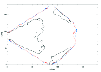
Figure 3: $\chi^{2}$ map for the fan beam model of the pulse width data on pulsar B. The $\chi^{2}$ contours are for the confidence levels of 1$\sigma$ (solid line), 2$\sigma$ (dotted line) and 3$\sigma$ (dashed line). The ‘plus’ sign on the left marks the minimum $\chi^{2}$ value, which should not be considered as a meaningful best-fit solution. The result was obtained for the outer traverse through the asymmetric beam ($\phi_{m1}=0$).

Fig. 3 presents the 1$\sigma$, 2$\sigma$ and 3$\sigma$ contours of $\chi^{2}$ on the $(\alpha,\lambda)$ plane, as calculated for the asymmetric outer case ($\phi_{m1}=0$, $\phi_{m2}<90^{\circ}$). It can be seen that for a very large range of $\alpha$ and $\lambda$ the model can reproduce the data with accuracy better than $2\sigma$. The pronounced bay of high $\chi^{2}$ on the right-hand side is caused by the condition of invisibility of pulsar B in the years 2009-2016, which resulted in the rejection of some good-precision fits. Without the invisibility condition, the $2\sigma$ and $3\sigma$ contours of $\chi^{2}$ have the shape of a undistorted rhombus.

The observations constrain both the observed width $W_{\rm obs}(t)$ and the roughly constant rate of width change $(dW/dt)_{\rm obs}$ at any moment when the pulsar B is detectable. The high capability of the model to adjust to both $W_{\rm obs}$ and $(dW/dt)_{\rm obs}$ can be most easily understood in the case of an orthogonal precession ($\lambda=90^{\circ}$, middle horizontal region of Fig. 3).

Since the observed profile is only a few degrees wide, our sightline must traverse the beam close to the dipole axis. Stated otherwise, the sightline’s smallest angular distance from the dipole axis, as measured within a given pulsar spin period, i.e., the impact angle $\beta=\zeta-\alpha$, must be generally small ($\beta\ll\alpha\sim\zeta$). The path of a sightline traverse through the beam may then be considered a straight line orthogonal to the main meridian, and the pulse width $W$ can be roughly approximated by:

$$W\approx\beta\tan\phi_{m2}/\sin\zeta\approx(\zeta(t)-\alpha)\tan\phi_{m2}/\sin\alpha.$$ (5)

Note that the small difference between $\zeta$ and $\alpha$ has been neglected in the denominator which takes into account the ‘small circle’ effect. Accordingly, the derivative of $W$ is

$$\frac{dW}{dt}\approx\frac{-\Omega_{p}\tan\phi_{m2}\sin\lambda\sin i\sin\Phi(t)}{\sin\alpha\sin\zeta(t)}.$$ (6)

In the case of the orthogonal precession ($\lambda\approx 90^{\circ}$), the near-orthogonal orbit inclination $i$ implies, through eq. (1), that $|\Phi(t)|\approx|\zeta(t)|$ and eq. (6) reduces to $|dW/dt|\approx|\Omega_{p}\tan\phi_{m2}|/\sin\alpha$. Thus for any $\alpha$ the model can reproduce an arbitrary value of $|dW/dt|$ through adjustment of the azimuthal beam separation ($\phi_{m2}$). In this orthogonal case ($\lambda\sim i\sim 90^{\circ}$), the width given by eq. (5) is simply equal to $W\approx|[\Omega_{p}(T_{0}-t)-\alpha]\tan\phi_{m2}|/\sin\alpha$ and for any set of $(\alpha,\phi_{m2},t)$ the width can be reproduced by adjustment of the impact angle through $T_{0}$.

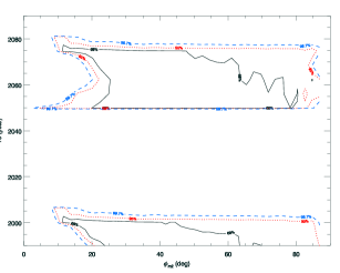
Figure 4: The map of $\chi^{2}$ on the $(\phi_{m2},T_{0})$ plane, calculated for the same case, and the same confidence levels as in the previous figure.

In the corners of Fig. 3, no combination of model parameters can reproduce the data. This can be understood by considering the case of $\lambda\ll 1$ rad and $\alpha\ll 1$ rad. The dipolar magnetosphere is then viewed roughly at a right angle with respect to the dipole axis ($\zeta\sim\theta_{m}\sim 90^{\circ}$) which implies $W\approx\phi_{m2}$ and $dW/dt\approx 0$. Thus, for the small precession angle the precession cannot ensure as steep variation of $W$ as observed. At a fixed $\alpha$, the value of $\lambda$ needs to be sufficiently large for the observed $dW/dt$ to appear at some precession phase. The parameters ($T_{0}$, $\phi_{m2}$) are then adjusted to allow the model to match the data. Beyond the rhombus region this is not possible.

The small-angle precession ($\lambda\ll 1$ rad) can only reproduce the data when $\alpha\approx 90^{\circ}$ (bottom and top corners of the rhombus). This is because the beam may now be viewed arbitrarily close to the dipole axis, so the tiny wiggling of the magnetosphere can change the small value of $\beta$ by a large factor.

It needs to be emphasized that the symmetric rhombus shape of the low-$\chi^{2}$ contours is characteristic of the orthogonal orbit inclination with respect to the line of sight ($i\approx 90^{\circ}$). For $i\neq 90^{\circ}$, the rhombus gets transformed into an elongated parallelogram.

The confidence contours ($68$, $95$ and $99.7$%) are also shown on the $(\phi_{m2},T_{0})$ map (Fig. 4). Again the observed $W$ can be reproduced with reasonable precision within a very large part of parameter space. There are horizontal bands visible, in which $T_{0}$ gives no acceptable solution. In these bands $\zeta$ changes with time in a wrong direction, causing $W$ to decrease with time, in contrast to the observations. The bands have the width of a half precession period and their borders do not depend on $\phi_{m2}$ because the evolution of $\zeta$ is fully determined by $\lambda$, $i$ and $T_{0}$ (eq. 1).

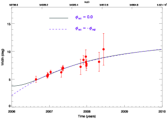
Figure 5: Nominally-best fit of the fan beam model to the pulse width data taken with GBT between Dec 24, 2003 and Jun 20, 2009 (PMK10). Solid line presents the asymmetric beam case marked with the cross in Fig. 3 ($\phi_{m1}=0$).

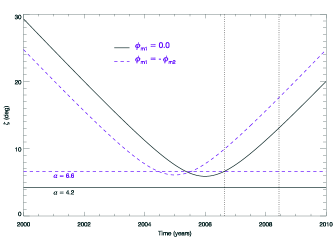
Figure 6: The viewing angle $\zeta$ as a function of time for the models shown in the previous figure (solid line: $\phi_{m1}$ = 0, dashed line: $\phi_{m2}=-\phi_{m1}$). Two vertical lines are drawn to indicate the region where the peak-separation data is available from the GBT.

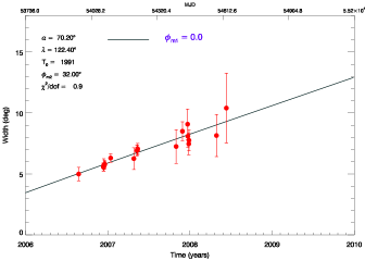
Figure 7: A fit to the bp1 data taking a random point within the rhombus-shaped part of the $\chi^{2}$ map.

Solid line in Figure 5 presents the ‘best’ fit curve of $W(t)$ for the asymmetric outer case ($\phi_{m1}=0$, $\phi_{m2}<90^{\circ}$). This fit may only be nominally considered as a best solution, because it is not statistically significant in comparison to the other models within the low $\chi^{2}$ region. The parameters of this fit are: $\alpha=4\degr.2$, $\lambda=82\degr.8$, $\phi_{m2}=13\degr.0$ and $T_{0}=2006$ yrs, thus giving $\chi^{2}/{\rm dof}=0.9$. An independent fit of the symmetric beam ($\phi_{m1}=-\phi_{m2}$, dashed line) provides similar parameters, this time with $\alpha=6\degr.6$. The dipole tilt seems to have suspiciously small value, however, by no means should these parameters be considered unique. Satisfactory data reproduction can be achieved for any point within the rhombus-shaped part of the $\chi^{2}$ map in Fig. 3. An example with randomly selected $\alpha$ and $\lambda$ is shown in Fig. 7. It has $\chi^{2}/{\rm dof}=0.95$.

Precessional changes of $\zeta$ that correspond to the nominally-best solutions of Fig. 5 are presented in Fig. 6. In both cases the line of sight approaches the magnetic dipole axis and then retreats. This behaviour is not universal: other solutions (for parameters at other locations within the rhombus) provide excellent data reproduction with the sightline passing far into the region on the other side of the magnetic axis.

When the fan beams are displaced to the other side of the magnetic pole (inner traverse case, i.e.: $\phi_{m1}=180^{\circ}$, $90^{\circ}<\phi_{m2}<180^{\circ}$), the results are analogous to those described above. The $\chi^{2}$ map on the $(\alpha,\lambda)$ plane is mirror reflected, i.e., the right-hand side bay in the rhombus of Fig. 3 appears in the left-hand side corner (i.e. at $\alpha\la 45^{\circ}$, and $\lambda\sim 90^{\circ}$). The low-$\chi^{2}$ bands on the $(\phi_{m2},T_{0})$ plane get mirror-reflected and shift vertically by a half of precession period (all values of $T_{0}$ are therefore consistent with the data).

The pulse width data for the other bright phase (bp2) have essentially the same character as the bp1 data. Therefore, the same analysis applied for bp2 gave similar results, i.e., the good data match within the large part of parameter space. For brevity, we skip the presentation of the bp2 results.

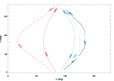
Figure 8: B’s reappearance time for the outer asymmetric case of Fig. 3. Note that the inner traverse case would produce a mirror-reflected image, with the early reappearance time and the missing rhombus corner located on the left hand side.

4.1 Reappearance time

Instead of a firm prediction for the reappearance time $t_{r}$, only a map of the parameter-dependent $t_{r}$ can be obtained. Fig. 8 presents contours of fixed $t_{r}$ on the $(\alpha,\lambda)$ map, calculated for the case presented in Fig. 3. For any pair of $(\alpha,\lambda)$, values of $\phi_{m2}$ and $T_{0}$ are kept at their best-fit magnitudes. For each such model, the range of viewing angles $(\zeta_{\rm vis}^{\rm min},\zeta_{\rm vis}^{\rm max})$ was determined based on the visibility of the pulsar B in the years 2003-2008. Then $t_{r}$ has been determined as the soonest moment when $\zeta(t)$ returns back into the visibility range.

As can be seen in Fig. 8, possible reappearance times (calculated for model parameters which can ensure good data match), range across most of the precession period (2017-2078). When moving from left to right in Fig. 8, (which was calculated for the outer traverse case), $t_{r}$ moves to earlier times. For the inner traverse (when beams are detectable at $\zeta<\alpha$, not shown) the $t_{r}$ contours look as a mirror reflection of Fig. 8, i.e., $t_{r}$ increases from the left-corner invisibility bay rightwards.

It may appear disturbing that possible values of the reappearance time, i.e. those which allow for good quality data match, span basically the full precession period (Fig. 8), whereas the possible precession phase $T_{0}$ is excluded within a half of $P_{\rm prec}$ (Fig. 4). The variations of $W(t)$ have a sinusoid-like form, with the ‘wavelength’ of the sinusoid fixed by the value of $P_{\rm prec}$. The only way to ensure sooner or later reappearance is to horizontally shift the sinusoid in $T_{0}$ (with a vertical adjustment to match the already-observed data). So there is a correspondence between $T_{0}$ and $t_{r}$, but a half of the $T_{0}$ values, seemingly needed to explain all $t_{r}$, is missing. This apparent paradox is caused by the mathematical properties of a sinusoid. Let us first consider $t_{r}$ coincident with the last data point (middle 2008). That is, consider a case in which immediately after the maximum observed width is reached ($W=W_{\rm max}$), the width starts to decrease with no disappearance of the B pulsar. Such behaviour would be reproduced with the maximum of the $W(t)$ sinusoid placed at $t_{r}$. However, if the supposed reappearance is now delayed by some $\Delta t_{r}$ (at which time the decreasing $W$ again takes on the same maximum-observed value as in the middle 2008), it is enough to shift the sinusoid horizontally by a two times smaller time interval ($\Delta T_{0}=\Delta t_{r}/2$) to both pass through $W(t_{r})=W_{\rm max}$ and match the real data points. A time displacement of the $W(t)$ curve produces two times larger delay of $t_{r}$. This is because the same values on both sides of the sinusoid’s peak are twice more distant from each other than from the phase of the peak. The nearly-half-period-long interval of $T_{0}$ in which the solution gives the correct sign of $dW/dt$ (see the bands in Fig. 4) is therefore sufficient to ensure all possible reappearance times.

4.2 Anticipated model constraints from future observations

It is interesting to estimate what constraints on the model parameters will become available when PSR J0727$-$3039B reappears at a certain moment in future. To study the problem we supplemented the GBT data on $W$ with a set of artificial data points, created in the following way: the original GBT data from Fig. 5 were reversed in time and shifted by an arbitrary time interval. This was done because the precession changes the viewing angle $\zeta$ in a sinusoid-like way, so a given range of monotonically changing $W$ is expected to appear twice per precession period, in a reversed time order. We added no data points with $W$ beyond the range observed so far, although the future, more sensitive radio telescopes may be capable to detect larger range of $W$.

Such experiment shows that the constraining capability of additional data is moderate. Only the precession phase ($T_{0}$) is tightly constrained down to about a year. The dipole tilt $\alpha$ can be limited with a precision of a few degrees, only when the B pulsar reappears close to the year 2036. In this specific case the low-$\chi^{2}$ contour on the $(\alpha,\lambda)$ plane is a narrow vertical stripe at $\alpha\sim 90^{\circ}$. However for $t_{r}$ departing from $2036$, the stripe bulges left or right on the $(\alpha,\lambda)$ plane, assuming an arc shape. At the same time the limits on $\alpha$ quickly become much less precise. For $t_{r}\sim 2078$ or $t_{r}\sim 2017$, the value of $\alpha$ (and $\lambda$) is basically unconstrained. This effect is similar to the well-known $\alpha$-$\zeta$ corellation in the polarisation angle fitting, which produces the arc-shaped $\chi^{2}$ contours on the $(\alpha,\zeta$) plane. Regardless of the actual reappearance time, the additional data do not provide any constraints on the precession angle $\lambda$, and the azimuthal separation of beams $\phi_{m,2}$.

It is interesting to ask if the future data allows us to discriminate between the conal-like and the fan-beam (patchy) models. In principle, the conal model seems to predict definite reappearance times (eg. $2035$ in Perera et al. 2010; $2034$, $2043$, and $2066$ in Lomiashvili & Lyutikov 2014), so if the pulsar reappears at a different time, only the fan beam model will stay consistent. However, the “conal” model has recently gained much flexibility: the emission ring became a part of an ellipse with an adjustable eccentricity and an adjustable circumpolar azimuth of its major axis.

5 Discussion

In terms of probability, the fan-shaped beam appears to be a successful model for the late-time evolution of the pulsar B profile. There is no need for fine-tuning, instead, there exists a large space of parameter values which can reproduce the observed roughly linear changes $W$. However, this flexibility prevents unique determination of pulsar and beam geometry. This ambiguity also holds for the question of reappearance time of pulsar B. Since the model parameters are not yet fully constrained, the model can adjust to any date on which the pulsar may appear in future. Such reappearance, along with new measurements of $W$ and $dW/dt$, would constrain some model parameters, provided the same radio beam is exposed to us again.

The ambiguity in well-fitting parameters tempted us to include the early data on PSR J0737$-$3039B from Burgay et al. (2005, see Fig. 2 therein). Unfortunately, for both observational and theoretical reasons, such analysis appears to be inconclusive.

There are the following observational problems. First, the bp1 profiles from the period Jun 2003 – Nov 2004 (bottom left corner of Fig. 2) cannot be unambiguously decomposed into two separate Gaussian components. Second, it is hard to decide if the bp1 components merge or a new (third) component is emerging, as suggested in Burgay et al. (2005). Third, the early bp2 profiles seem to exhibit different shape evolution, with a nearly fixed peak-to-peak separation, but the leading component decreasing in strength. This may indicate that our sightline probes widely different beam portions in bp1 and bp2, because of orbital-dependent distortions of magnetosphere (see Lomiashvili & Lyutikov 2014), or that the beam shape itself depends on orbital phase.

On the theoretical side, the simplest model such as the one used in the previous section meets serious difficulties with simultaneous reproduction of both the early (2003-Nov 2004) and late time evolution (2006-2008). The unresolved or single shape of profile in 2005 can be interpreted as an overlapping emission from two nearby streams (Fig. 9c), however, the large and roughly constant peak-to-peak separation of bp2 components in the early period cannot be understood if the fan beam model is limited to such two beams only. The conal model is even less likely to explain this, because of its lack of flexibility which results from the conal beam symmetry. The fan beam model, on the other hand, still lacks the physical framework and offers some flexibility in choosing the beam geometry.

An important question is whether the beam responsible for the early-period profile is located on the same side of the magnetic axis as the late-season beam, i.e., whether our line of sight has passed over the magnetic pole in 2005 (by moving meridionally, eg. from the outer- to inner-traverse side) As is the case in Fig. 9, the system of fan beams is possibly different (asymmetric) on both sides of the magnetic pole (equatorward vs poleward) which leaves lots of flexibility for the fan beam model to reproduce different pulse behaviour in the early and late period. Unfortunately, through the modelling of the late-time data from PMK10, it is not possible to distinguish between these scenarios. When the fan-beam model of Sect. 2 is used, these late-time data can be well reproduced by solutions of both types, namely those for which our sightline moves across the pole, but also those with the sightline retreating back after a close approach to the pole (without the pole crossing).

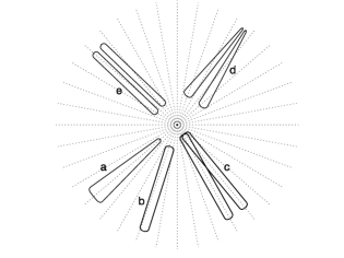
Figure 9: Various types of sky-projected fan beams. Dotted lines mark the dipolar $B$-field, and the central dot is the magnetic dipole axis. a) Single beam which gets wider away from the axis, as caused by the spreading $B$-field. b) Single beam of a fixed width. c) System of two fan beams which diverge along with the spreading $B$-field and overlap near the dipole axis. d) Bifurcated beam with lobes converging away from the dipole axis. e) Bifurcated beam with a fixed distance between its lobes. The latter two beams (d and e) are typical of the X-mode curvature radiation. Case e corresponds to a fixed radius of curvature of electron trajectory.

The modelling freedom is even larger than that, because the physical origin of profiles’ double form is not known. Aside from the polar-tube-related conal interpretations, multiple fan-beam types are possible, with various transverse emissivity profiles, and with different arrangement of fan-shaped subbeams (cartoon examples are shown in Fig. 9). Divergence of the magnetic field suggests that beams become wider at larger distance from the dipole axis (Fig. 9a), and this effect is visible in the three dimensional simulations of Wang et al. (2014, see figs. 5-12 therein). However, the fan beam observed in PSR J1906$+$0746 (Desvignes et al. 2012) does not show much broadening. This is not surprising, because the local magnetospheric emissivity depends on the emitted spectrum and the latter is sensitive to the energy distribution of emitting particles. The emitted intensity is then dependent on the acceleration and cooling history of the radiating charges, which may be different at different lateral locations in the emission region. In the case of the curvature radiation at standard conditions (charge Lorentz factor $\gamma\sim 10^{2}$, curvature radius of their trajectory $\rho\sim 10^{7}$ cm) the curvature radiation spectrum barely reaches the observed $\sim 1$ GHz band. Therefore, any transverse differences in acceleration or cooling can influence the observed width of the fan beam in a latitude-dependent way. If the emission region has the form of a dense curved stream of particles (such as shown in Fig. 12 of Dyks & Rudak 2015) then the association of plasma density with the emitted frequency (also present in the radius-to-frequency mapping) will move the site of strong radio emission to the center of the stream (at increasing altitude). It is for such observational and theoretical reasons, that the latitude-dependence of the fan-beam width should be considered mostly unconstrained, or at least not only determined by the spread of the dipolar magnetic field. A fixed-width example of such an arbitrary beam is presented in Fig. 9b.

Double structure of the observed profile may have various reasons. It may be caused by emission from two, mostly independent, nearby streams, producing a system consisting of two fan beams (Fig. 9c). Alternatively, it may result from a single stream which itself emits a split-fan beam (Fig. 9d). In this case the bifurcation may have either the micro- or macroscopic origin. The curvature radiation in the extraordinary mode is a known mechanism which produces this type of a beam (see Fig. 3 in Gil et al. 2004). The angular separation of emission lobes in the beam is proportional to $\rho^{-1/3}$ (eq. 3 in Dyks & Rudak 2012), so in the dipolar field it slowly decreases with the distance from the dipole axis, as marked in Fig. 9d. If the changes of $\rho$ along the particle trajectory are negligible, the beam 9e is expected. In the macroscopic case the split-fan form may result from the aforementioned transverse density profile of the stream (Fig. 12 in Dyks & Rudak 2015). A shallow bifurcation could possibly appear also for a stream in which most plasma is gyrating at a preferred pitch angle.

Given all these uncertainties (the limited time span and quality of data, the large space of well fitting parameters, the model flexibility in terms of the number and location of fan beams, and the uncertain fan beam origin and geometry), more data for a larger interval of precession phase is required to answer the question on whether the fan beams can explain the apparently different pulse behaviour observed in 2003 and 2007.

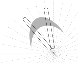
Figure 10: A cartoon comparing the horseshoe beam fitted by Lomiashvili & Lyutikov (2014; grey arc) to a hypothetical system of two fan beams (solid line contours). Because of roughly similar location within the magnetosphere, the beams are suspected to have similar orbital visibility. Since open sides of the beams point in opposite directions, the observed increase in $W$ requires an opposite precession direction for each beam type.

This paper has made use of the ‘static-shape’ dipolar magnetic field, undistorted by the pulsar A’s wind. Such field geometry cannot be used to model the visibility of PSR J0737$-$3039B in specific orbital phase intervals. Lomiashvili & Lyutikov (2014) carefully modelled the system with a wind-distorted field. They show that the orbital visibility can be reproduced within a unique interval of precession phase, although the precession direction needs to be opposite to that predicted by the general relativity. Their result is based on a beam of a modified-cone type: it is a piece of elliptic arc resembling a horseshoe, with its open side directed towards the magnetic axis. Let us consider the case in which the horseshoe beam (grey contour in Fig. 10) is replaced with a V-shaped fan beam system considered in this paper (solid line contours in Fig. 10). Let the fan beam be located within a similar region of magnetosphere as the horseshoe beam (on the same side of the magnetic axis, within a similar interval of magnetic azimuths and colatitudes), except the beam’s open side is now pointing away from the dipole axis. Because of the similar magnetospheric location, the fan beam should still be capable of reproducing the orbital visibility. However, since the open side of the fan beam is pointing away from the dipole axis, the observed increase in $W$ can only be reproduced for an opposite precession direction (consistent with the general relativity). It is therefore reasonable to expect that the V-shaped beam pointing towards the dipole axis (and directing its open side away from it) can reproduce the bright orbital phases in a more natural way than the conal-like horseshoe beam (i.e., in consistency with the general relativity).

Lomiashvili & Lyutikov (2014) have shown that the radio beam geometry is not very sensitive to the wind distortion of the magnetosphere: parameters of their horseshoe beam are consistent with those found by PMK10 for the static shape (pure) dipole. This suggests that our inferences on the performance of the fan beam geometry should prevail in the case of the wind-distorted magnetic field.

6 Summary

This study shows that the late-time secular changes of pulsed emission from PSR J0737-3039B can be explained in the framework of the fan-beam model. The estimated space of acceptable model parameters is quite large as compared to that for the conal-beam model. However, at least some parameters should become more tightly constrained when the information about the reappearance of the pulse and more data on $W$ is provided by future observations.

It is suggested here that the radio beam of PSR J0737$-$3039 consists of elongated patches with mostly azimuthal orientation. The same or similar geometry has appeared valid for two other precessing objects (Manchester et al., 2010; Desvignes et al., 2012). It is remarkable that pulsars with patchy or fan beams make up for some 50% of precessing objects, for which beam mapping has appeared feasible so far.

References

- Barker & O’Connell (1975) Barker, B. M., & O’Connell, R. F. 1975, Phys. Rev. D, 12, 329
- Breton et al. (2008) Breton, R. P., Kaspi, V. M., Kramer, M., et al. 2008, Science, 321, 104
- Burgay et al. (2003) Burgay, M., D’Amico, N., Possenti, A., et al. 2003, Nature, 426, 531
- Burgay et al. (2005) Burgay, M., Possenti, A., Manchester, R. N., et al. 2005, ApJL, 624, L113
- Chen & Wang (2014) Chen, J. L., & Wang, H. G. 2014, ApJS, 215, 11
- Clifton & Weisberg (2008) Clifton, T., & Weisberg, J. M. 2008, ApJ, 679, 687
- Coles et al. (2005) Coles, W. A., McLaughlin, M. A., Rickett, B. J., Lyne, A. G., & Bhat, N. D. R. 2005, ApJ, 623, 392
- Desvignes et al. (2012) Desvignes, G., Kramer, M., Cognard, I., et al. 2012, in Proceedings of the International Astronomical Union, Vol. 8, Neutron Stars and Pulsars: Challenges and Opportunities after 80 years, 199–202
- Dyks & Pierbattista (2015) Dyks, J., & Pierbattista, M. 2015, MNRAS, 454, 2216
- Dyks & Rudak (2012) Dyks, J., & Rudak, B. 2012, MNRAS, 420, 3403
- Dyks & Rudak (2015) —. 2015, MNRAS, 446, 2505
- Dyks et al. (2010) Dyks, J., Rudak, B., & Demorest, P. 2010, MNRAS, 401, 1781
- Dyks et al. (2016) Dyks, J., Serylak, M., Oslowski, S., et al. 2016, ArXiv e-prints, arXiv:1608.00770
- Gil et al. (2004) Gil, J., Lyubarsky, Y., & Melikidze, G. I. 2004, ApJ, 600, 872
- Karastergiou & Johnston (2007) Karastergiou, A., & Johnston, S. 2007, MNRAS, 380, 1678
- Kramer (1998) Kramer, M. 1998, ApJ, 509, 856
- Kramer et al. (2006) Kramer, M., Stairs, I. H., Manchester, R. N., et al. 2006, Science, 314, 97