The Higgs boson decay into $ZZ$ decaying to identical fermion pairs

Abstract

In order to investigate various decay channels of the Higgs boson $h$ or the hypothetical dilaton, we consider a neutral particle $X$ with zero spin and arbitrary $CP$ parity. This particle can decay into two off-mass-shell $Z$ bosons ($Z_{1}^{*}$ and $Z_{2}^{*}$) decaying to identical fermion-antifermion pairs ($f\bar{f}$): $X\to Z_{1}^{*}Z_{2}^{*}\to f\bar{f}f\bar{f}$. We derive analytical formulas for the fully differential width of this decay and for the fully differential width of $h\to Z_{1}^{*}Z_{2}^{*}\to 4\ell$ ($4\ell$ stands for $4e$, $4\mu$, or $2e2\mu$). Integration of these formulas yields some Standard Model histogram distributions of the decay $h\to Z_{1}^{*}Z_{2}^{*}\to 4\ell$ which are compared with corresponding Monte Carlo simulated distributions obtained by ATLAS and with ATLAS experimental data.

PACS numbers: 12.15.Ji, 12.60.Fr, 14.80.Bn, 14.80.Ec

1 Introduction

The boson $h$ discovered [1, 2] in 2012 by the CMS and ATLAS collaborations was reported to have a mass about 125 GeV and some decay modes predicted for the Standard Model (SM) Higgs boson. Since that time, the observed particle, called the Higgs boson, has been intensively studied (see, for example, Refs. 3, 4, 5, 6, 7, 8, 9, 10, 11, 12, 13, 14, 15, 16, 17, 18, 19, 20, 21, 22, 23, 24, 25, 26, 27). A main goal of experiments on the Higgs boson physics has been to prove or disprove the hypothesis that $h$ is the SM Higgs boson. Apart from the decay channels, the SM predicts that $h$ has $J^{CP}=0^{++}$. The followed thorough analysis has fine-tuned the mass of $h$, which is $125.09\pm 0.24$ GeV according to Ref. 28, and has yielded some information on its spin and its $CP$ parity.

In particular, the observation of the $h\to ZZ$ and $h\to W^{-}W^{+}$ modes (see, for example, Ref. 29) means that the Higgs boson spin is zero, one, or two while the fact that $h$ decays [29] to $\gamma\gamma$ and the Landau-Yang theorem exclude the spin-one variant. Further, the analyses presented in Ref. 30, 31 rule out many spin-two hypotheses at a 99% confidence level (CL) or higher. Therefore, we conclude that the spin of the Higgs boson is zero with a probability of about 99%.

To clarify the $CP$ properties of $h$, in Ref. 32 we study the decay of a spin-zero particle $X$ into two off-mass-shell $Z$ bosons $Z_{1}^{*}$ and $Z_{2}^{*}$. Since $X$ is defined as an elementary neutral particle with zero spin, our study applies to the Higgs boson. Moreover, it can apply to the dilaton if this boson actually exists.

The amplitude of the decay $X\to Z_{1}^{*}Z_{2}^{*}$ depends (see Eq. (4) in Ref. 32) on 3 complex-valued functions of the invariant masses of $Z_{1}^{*}$ and $Z_{2}^{*}$. These functions determine the $CP$ properties of the boson $X$ and are called the $XZZ$ couplings. Using the CMS and ATLAS experimental data on the decay $h\to Z_{1}^{*}Z_{2}^{*}\to 4\ell$ (where $4\ell$ stands for $4e$, $4\mu$, or $2e2\mu$), these collaborations in Refs. 30, 31, 29 and we in Ref. 32 have obtained some constraints on the $hZZ$ couplings. These constraints demonstrate that $h$ is not a $CP$-odd state and it may be the SM Higgs boson, another $CP$-even state, or a boson with indefinite $CP$ parity. Besides, as shown in Ref. 32, a non-zero imaginary part of the $hZZ$ couplings is not excluded, which can be related to small loop corrections and possibly to a non-Hermiticity of the $hZZ$ interaction.

Thus, the $CP$ parity of the Higgs boson is not yet fully ascertained. Moreover, in some supersymmetric extensions of the SM there are [33, 34, 35] neutral bosons with negative or indefinite $CP$ parity. That is why it is now important to establish the $CP$ properties of the Higgs boson.

Aiming at that, we consider the decay of the particle $X$ into $Z_{1}^{*}$ and $Z_{2}^{*}$ which then decay to fermion-antifermion pairs $f_{1}\bar{f}_{1}$ and $f_{2}\bar{f}_{2}$ respectively. While in Ref. 32 we study in detail the decays with the non-identical fermions, $f_{1}\neq f_{2}$, in the present paper the case $f_{1}=f_{2}$ is under investigation. The masses of the fermions $f_{1}$ and $f_{2}$ are neglected in both papers.

We are motivated to consider the decay into identical fermions by the following. In Refs. 31, 30 the CMS and ATLAS collaborations analyze 95 events $h\to Z_{1}^{*}Z_{2}^{*}\to 4\ell$. 53 of them are the decays to identical leptons, namely to $4e$ or $4\mu$. In spite of the fact that the decays to the identical leptons make up about 55% of the measured decays $h\to Z_{1}^{*}Z_{2}^{*}\to 4\ell$, the distributions of the former decays have not been properly analytically studied.

The SM total widths of the decays into identical fermions are studied in Refs. 36, 37 and are calculated in Ref. 38. Some distributions of the decay $X\to Z_{1}^{*}Z_{2}^{*}\to 4\ell$ are plotted in Ref. 30, 31 for the SM Higgs boson and some spin-zero states beyond the SM. In the present paper we perform a more general study and consider the decay $X\rightarrow Z_{1}^{*}Z_{2}^{*}\rightarrow f\bar{f}f\bar{f}$ with allowance for all the possible $CP$ properties of the particle $X$.

In Sec. 2 we derive an analytical formula for the fully differential width of the decay to identical fermions. Section 3 shows a comparison of some distributions of the decay to identical leptons with those for the decay into non-identical ones. For this comparison we obtain an exact analytical formula for a certain differential width of the decay to non-identical fermions (see B). We analyze the usefulness of all the compared distributions for obtaining constraints on the $hZZ$ couplings. In Sec. 4 we derive some SM histogram distributions of the decay $h\to Z_{1}^{*}Z_{2}^{*}\to 4\ell$ by Monte Carlo (MC) integration and compare them with the corresponding simulations presented in Ref. 30 and with the experimental distributions from Ref. 30.

2 The fully differential width

We consider a neutral particle $X$ with zero spin and arbitrary $CP$ parity. It can decay into two fermion-antifermion pairs, $f_{1}\bar{f}_{1}$ and $f_{2}\bar{f}_{2}$, through the two off-mass-shell $Z$ bosons ($Z_{1}^{*}$ and $Z_{2}^{*}$):

$$X\rightarrow Z_{1}^{*}Z_{2}^{*}\rightarrow f_{1}\bar{f}_{1}f_{2}\bar{f}_{2}.$$ (1)

If $m_{X}\in(4m_{b},2m_{t}]$ ($m_{X}$ is the mass of the particle $X$, $m_{b}$ is the mass of the $b$ quark, $m_{t}$ is the mass of the $t$ quark), which holds for $X=h$, then $f_{j}=e^{-},\mu^{-},\tau^{-},\nu_{e},\nu_{\mu},\nu_{\tau},u,c,d,s,b$. If $m_{X}>4m_{t}$, which is possible [39] if $X$ is the dilaton, then $f_{j}$ can be the top quark as well.

In Ref. 32 we considered decays

$$X\rightarrow Z_{1}^{*}Z_{2}^{*}\rightarrow f_{1}\bar{f}_{1}f_{2}\bar{f}_{2},\qquad f_{1}\neq f_{2}$$ (2)

at the tree level.

The present paper shows our analysis of decay (1) in the case of the identical fermions, $f_{1}=f_{2}\equiv f$:

$$X\rightarrow Z_{1}^{*}Z_{2}^{*}\rightarrow f\bar{f}f\bar{f}.$$ (3)

The matrix element of decay (3) is

$$M_{iden}=M-\tilde{M},$$ (4)

where the matrix elements $M$ and $\tilde{M}$ correspond to the diagrams (a) and (b) in Fig. 1 respectively. Namely,

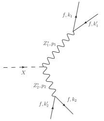
a

b

Figure 1: The Feynman diagrams contributing to the matrix element of decay (3).

$$M= \frac{i}{(a_{1}-m_{Z}^{2}+im_{Z}\Gamma_{Z})(a_{2}-m_{Z}^{2}+im_{Z}\Gamma_{Z})}\sum_{\lambda_{1},\lambda_{2}=-1,0,1}A_{X\to Z_{1}^{*}Z_{2}^{*}}(p_{1},p_{2},\lambda_{1},\lambda_{2})$$

$$\times A_{Z\to f\bar{f}}(k_{1},k_{1}^{\prime},\lambda_{f_{1}},\lambda_{\bar{f}_{1}},\lambda_{1})A_{Z\to f\bar{f}}(k_{2},k_{2}^{\prime},\lambda_{f_{2}},\lambda_{\bar{f}_{2}},\lambda_{2}),$$

$$\tilde{M}= \frac{i}{(\tilde{a}_{1}-m_{Z}^{2}+im_{Z}\Gamma_{Z})(\tilde{a}_{2}-m_{Z}^{2}+im_{Z}\Gamma_{Z})}\sum_{\lambda_{1},\lambda_{2}=-1,0,1}A_{X\to Z_{1}^{*}Z_{2}^{*}}(\tilde{p}_{1},\tilde{p}_{2},\lambda_{1},\lambda_{2})$$

$$\times A_{Z\to f\bar{f}}(k_{1},k_{2}^{\prime},\lambda_{f_{1}},\lambda_{\bar{f}_{2}},\lambda_{1})A_{Z\to f\bar{f}}(k_{2},k_{1}^{\prime},\lambda_{f_{2}},\lambda_{\bar{f}_{1}},\lambda_{2}),$$ (5)

where

• $k_{1}$ and $k_{1}^{\prime}$ ($k_{2}$ and $k_{2}^{\prime}$) are the 4-momenta of the particles $f_{1}$ and $\bar{f}_{1}$ ($f_{2}$ and $\bar{f}_{2}$) in the rest frame of $X$;

• $p_{1}\equiv k_{1}+k_{1}^{\prime}$ and $p_{2}\equiv k_{2}+k_{2}^{\prime}$ are the 4-momenta of $Z_{1}^{*}$ and $Z_{2}^{*}$ respectively in the rest frame of $X$ in diagram Fig. 1 (a);

• $a_{j}\equiv p_{j}^{2}$;

• $m_{Z}$ and $\Gamma_{Z}$ are respectively the pole mass and the total width of the $Z$ boson;

• $A_{X\to Z_{1}^{*}Z_{2}^{*}}(p_{1},p_{2},\lambda_{1},\lambda_{2})$ is the amplitude of the decay $X\to Z_{1}^{*}Z_{2}^{*}$ where $p_{j}$ and $\lambda_{j}$ are respectively the momentum and the helicity of the boson $Z_{j}^{*}$ in the rest frame of $X$;

• $A_{Z\to f\bar{f}}(k,k^{\prime},\lambda_{f},\lambda_{\bar{f}},\lambda)$ is the amplitude of the decay $Z\to f\bar{f}$ where $k$ and $\lambda_{f}$ ($k^{\prime}$ and $\lambda_{\bar{f}}$) are respectively the momentum and the polarization of $f$ ($\bar{f}$) in the rest frame of $Z$, $\lambda$ is the helicity of decaying $Z$;

• $\tilde{p}_{1}\equiv k_{1}+k_{2}^{\prime}$ and $\tilde{p}_{2}\equiv k_{2}+k_{1}^{\prime}$ are the 4-momenta of $Z_{1}^{*}$ and $Z_{2}^{*}$ respectively in the rest frame of $X$ in diagram Fig. 1 (b);

• $\tilde{a}_{j}\equiv\tilde{p}_{j}^{2}$.

From the conservation of the energy-momentum 4-vectors we find all the possible values of $a_{1}$ and $a_{2}$:

$$4m_{f_{1}}^{2}<a_{1}<(m_{X}-2m_{f_{2}})^{2},\qquad 4m_{f_{2}}^{2}<a_{2}<(m_{X}-\sqrt{a_{1}})^{2},$$ (6)

where $m_{f_{j}}$ is the mass of the fermion $f_{j}$.

The amplitude $A_{X\to Z_{1}^{*}Z_{2}^{*}}(p_{1},p_{2},\lambda_{1},\lambda_{2})$ is [32]

$$A_{X\rightarrow Z_{1}^{*}Z_{2}^{*}}(p_{1},p_{2},\lambda_{1},\lambda_{2})= g_{Z}\Biggl{(}a_{Z}(a_{1},a_{2})(e_{1}^{*}\cdot e_{2}^{*})+\frac{b_{Z}(a_{1},a_{2})}{m_{X}^{2}}(e_{1}^{*}\cdot p_{X})(e_{2}^{*}\cdot p_{X})$$

$$+i\frac{c_{Z}(a_{1},a_{2})}{m_{X}^{2}}\varepsilon_{\mu\nu\rho\sigma}p_{X}^{\mu}(p_{1}^{\nu}-p_{2}^{\nu})(e_{1}^{\rho})^{*}(e_{2}^{\sigma})^{*}\Biggr{)},$$ (7)

where $g_{Z}\equiv 2\sqrt{\sqrt{2}G_{F}}m_{Z}^{2}$, $G_{F}$ is the Fermi constant, $a_{Z}(a_{1},a_{2})$, $b_{Z}(a_{1},a_{2})$, and $c_{Z}(a_{1},a_{2})$ are some complex-valued dimensionless functions of $a_{1}$ and $a_{2}$, $e_{j}\equiv e(p_{j},\lambda_{j})$ with $e(p,\lambda)$ being the polarization 4-vector of the $Z$ boson with a momentum $p$ and a helicity $\lambda$, $p_{X}\equiv p_{1}+p_{2}=\tilde{p}_{1}+\tilde{p}_{2}=(m_{X},\vec{0})$ is the 4-momentum of the boson $X$ in its own rest frame, $\varepsilon_{\mu\nu\rho\sigma}$ is the Levi-Civita symbol ($\varepsilon_{0123}=1$).

The values of the couplings $a_{Z}$, $b_{Z}$, and $c_{Z}$ reflect the $CP$ properties of the particle $X$. Specifically, at the tree level the correspondence shown in Table 2 takes place.

The $CP$ parity of the particle $X$ for various values of $a_{Z}$, $b_{Z}$, and $c_{Z}$. $CP_{X}$ $a_{Z}$ $b_{Z}$ $c_{Z}$ 1 any any 0 $-1$ 0 0 $\neq$ 0 indefinite $\neq$ 0 any $\neq$ 0 any $\neq 0$ $\neq 0$

For the SM Higgs boson the loop corrections change slightly the tree-level values $a_{Z}=1$, $b_{Z}=0$, $c_{Z}=0$ (see, for example, Refs. 40, 41, 31, 42). In particular, the SM electroweak radiative diagrams tune the value of the coupling $b_{Z}$, beginning from the next-to-leading order, while a contribution to $c_{Z}$ appears at the three-loop level, so that $|b_{Z}|\approx 10^{-2}$ and $|c_{Z}|\approx 10^{-11}$ (see Ref. 43). Physics beyond the SM is the additional source of a possible deviation from the values $a_{Z}=1$, $b_{Z}=0$, $c_{Z}=0$.

Calculating Lorentz-invariant amplitude (2) in the rest frame of $X$, we derive that

$$A_{X\rightarrow Z_{1}^{*}Z_{2}^{*}}(p_{1},p_{2},\pm 1,\pm 1)=g_{Z}\left(a_{Z}(a_{1},a_{2})\pm c_{Z}(a_{1},a_{2})\frac{k}{m_{X}^{2}}\right),$$

$$A_{X\rightarrow Z_{1}^{*}Z_{2}^{*}}(p_{1},p_{2},0,0)=-g_{Z}\left(a_{Z}(a_{1},a_{2})\frac{m_{X}^{2}-a_{1}-a_{2}}{2\sqrt{a_{1}a_{2}}}+b_{Z}(a_{1},a_{2})\frac{k^{2}}{4m_{X}^{2}\sqrt{a_{1}a_{2}}}\right),$$

$$A_{X\rightarrow Z_{1}^{*}Z_{2}^{*}}(p_{1},p_{2},\lambda_{1},\lambda_{2})=0,\qquad\lambda_{1}\neq\lambda_{2},$$ (8)

where $k(a_{1},a_{2})\equiv\lambda^{1/2}(m_{X}^{2},a_{1},a_{2})$, $\lambda(x,y,z)\equiv x^{2}+y^{2}+z^{2}-2xy-2xz-2yz$.

We take the amplitude $A_{Z\to f\bar{f}}(k,k^{\prime},\lambda_{f},\lambda_{\bar{f}},\lambda)$ from the SM (see, for example, Ref. 44).

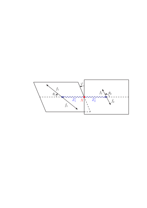
Figure 2: The kinematics of decay (1). We show the momenta of $Z_{1}^{*}$ and $Z_{2}^{*}$ in the rest frame of $X$ while the momenta of $f_{1}$ and $\bar{f}_{1}$ ($f_{2}$ and $\bar{f}_{2}$) are shown in the rest frame of $Z_{1}^{*}$ ($Z_{2}^{*}$).

Further, to describe decay (1), let us introduce the following angles (see Fig. 2): $\theta_{1}$ ($\theta_{2}$) is the angle between the momentum of $Z_{1}^{*}$ ($Z_{2}^{*}$) in the rest frame of $X$ and the momentum of $f_{1}$ ($f_{2}$) in the rest frame of $Z_{1}^{*}$ ($Z_{2}^{*}$) (in other words, $\theta_{1}$ ($\theta_{2}$) is the polar angle of the fermion $f_{1}$ ($f_{2}$)) and $\varphi$ is the azimuthal angle between the planes of the decays $Z_{1}^{*}\rightarrow f_{1}\bar{f}_{1}$ and $Z_{2}^{*}\rightarrow f_{2}\bar{f}_{2}$. For decay (3), we can arbitrarily choose the $Z$ boson which we will call $Z_{1}^{*}$, and then we will refer to the other $Z$ boson as $Z_{2}^{*}$.

As for $\tilde{a}_{1}$ and $\tilde{a}_{2}$, an explicit calculation yields

$$\tilde{a}_{1}=\frac{m_{X}^{2}-a_{1}-a_{2}}{4}(1-\cos\theta_{1}\cos\theta_{2})+\frac{\sqrt{a_{1}a_{2}}}{2}\sin\theta_{1}\sin\theta_{2}\cos\phi+\frac{k}{4}(\cos\theta_{1}-\cos\theta_{2}),$$

$$\tilde{a}_{2}=\frac{m_{X}^{2}-a_{1}-a_{2}}{4}(1-\cos\theta_{1}\cos\theta_{2})+\frac{\sqrt{a_{1}a_{2}}}{2}\sin\theta_{1}\sin\theta_{2}\cos\phi+\frac{k}{4}(\cos\theta_{2}-\cos\theta_{1}).$$ (9)

The expression for the amplitude $A_{X\to Z_{1}^{*}Z_{2}^{*}}(\tilde{p}_{1},\tilde{p}_{2},\lambda_{1},\lambda_{2})$ is analogous to Eq. (2):

$$A_{X\rightarrow Z_{1}^{*}Z_{2}^{*}}(\tilde{p}_{1},\tilde{p}_{2},\lambda_{1},\lambda_{2})= g_{Z}\Biggl{(}a_{Z}(\tilde{a}_{1},\tilde{a}_{2})(\tilde{e}_{1}^{*}\cdot\tilde{e}_{2}^{*})+\frac{b_{Z}(\tilde{a}_{1},\tilde{a}_{2})}{m_{X}^{2}}(\tilde{e}_{1}^{*}\cdot p_{X})(\tilde{e}_{2}^{*}\cdot p_{X})$$

$$+i\frac{c_{Z}(\tilde{a}_{1},\tilde{a}_{2})}{m_{X}^{2}}\varepsilon_{\mu\nu\rho\sigma}p_{X}^{\mu}(\tilde{p}_{1}^{\nu}-\tilde{p}_{2}^{\nu})(\tilde{e}_{1}^{\rho})^{*}(\tilde{e}_{2}^{\sigma})^{*}\Biggr{)},$$ (10)

where $\tilde{e}_{j}=e(\tilde{p}_{j},\lambda_{j})$. Calculating $A_{X\to Z_{1}^{*}Z_{2}^{*}}(\tilde{p}_{1},\tilde{p}_{2},\lambda_{1},\lambda_{2})$ in the rest frame of $X$, we get

$$A_{X\rightarrow Z_{1}^{*}Z_{2}^{*}}(\tilde{p}_{1},\tilde{p}_{2},\pm 1,\pm 1)=g_{Z}\left(a_{Z}(\tilde{a}_{1},\tilde{a}_{2})\pm c_{Z}(\tilde{a}_{1},\tilde{a}_{2})\frac{2}{m_{X}}|\mathbf{k}_{1}+\mathbf{k}_{2}^{\prime}|\right),$$

$$A_{X\rightarrow Z_{1}^{*}Z_{2}^{*}}(\tilde{p}_{1},\tilde{p}_{2},0,0)=-\frac{g_{Z}}{4\sqrt{\tilde{a}_{1}\tilde{a}_{2}}}\Biggl{(}a_{Z}(\tilde{a}_{1},\tilde{a}_{2})\Bigl{(}m_{X}^{2}+a_{1}+a_{2}+(m_{X}^{2}-a_{1}-a_{2})$$

$$\times\cos\theta_{1}\cos\theta_{2}-2\sqrt{a_{1}a_{2}}\sin\theta_{1}\sin\theta_{2}\cos\phi\Bigr{)}+b_{Z}(\tilde{a}_{1},\tilde{a}_{2})\cdot 4|\mathbf{k}_{1}+\mathbf{k}_{2}^{\prime}|^{2}\Biggr{)},$$

$$A_{X\rightarrow Z_{1}^{*}Z_{2}^{*}}(\tilde{p}_{1},\tilde{p}_{2},\lambda_{1},\lambda_{2})=0,\qquad\lambda_{1}\neq\lambda_{2},$$ (11)

where

$$|\mathbf{k}_{1}+\mathbf{k}_{2}^{\prime}|^{2}= \frac{a_{1}+a_{2}}{4}-\frac{\sqrt{a_{1}a_{2}}}{2}\sin\theta_{1}\sin\theta_{2}\cos\phi+\frac{k^{2}}{16m_{X}^{2}}(\cos^{2}\theta_{1}+\cos^{2}\theta_{2})$$

$$+\frac{\cos\theta_{1}\cos\theta_{2}}{8m_{X}^{2}}(m_{X}^{4}-(a_{1}-a_{2})^{2}).$$ (12)

Using Eqs. (4), (2), (2), (2), and (2), we derive Eq. (A) (see A).

3 Invariant mass and angular distributions

Integrating Eq. (A) numerically, we can obtain some distributions of decay (3). Moreover, numerical integration of Eq. (5) in Ref. 32 yields distributions for decay (2). In Figs. 3 and 4 we compare certain distributions of (3) with those of (2). We define the weak mixing angle as $\theta_{W}\equiv\arcsin\sqrt{1-m_{W}^{2}/m_{Z}^{2}}$, where $m_{W}$ is the mass of the $W$ boson, and use the values of the constants in Table 3 neglecting their experimental uncertainties.

The values of the Fermi constant, of the masses of $h$, $Z$, $W$, and of the total width of $Z$ from Ref. 45. $G_{F}=1.1663787(6)\times 10^{-5}~{}{\rm GeV}^{-2}$ $m_{h}=125.7(4)~{}{\rm GeV}$ $m_{Z}=91.1876(21)~{}{\rm GeV}$ $m_{W}=80.385(15)~{}{\rm GeV}$ $\Gamma_{Z}=2.4952(23)~{}{\rm GeV}$

First, we show the SM distribution $\frac{1}{\Gamma}\frac{d^{2}\Gamma}{da_{1}da_{2}}$ for any decay $h\to Z_{1}^{*}Z_{2}^{*}\to f_{1}\bar{f}_{1}f_{2}\bar{f}_{2}$ with $f_{1}$ different from $f_{2}$ (see Fig. 3a) and that for any decay $h\to Z_{1}^{*}Z_{2}^{*}\to 4l$ where $l$ stands for $e$, $\mu$, or $\tau$ (see Fig. 3b). We see peaks at $\sqrt{a_{1}}=m_{Z}$ or $\sqrt{a_{2}}=m_{Z}$ and a flat surface outside the peaks for either dependence. For the decay into non-identical fermions the SM values of $\frac{1}{\Gamma}\frac{d^{2}\Gamma}{da_{1}da_{2}}$ on the peaks are about 120 times greater than the values on the “plateau” (the square $\sqrt{a_{1}},\sqrt{a_{2}}\lesssim 50$ GeV). However, for the decay into identical leptons this ratio varies from 3 to 55 if we take $\sqrt{a_{1}}=m_{Z}$, $\sqrt{a_{2}}=\frac{1}{2}(m_{h}-m_{Z})$ as the indicative point on the peak and on the plateau we consider the points on the line $\sqrt{a_{1}}=\sqrt{a_{2}}$ from $\sqrt{a_{1}}=1$ GeV to $\sqrt{a_{1}}=59$ GeV. Moreover, the SM probability that in a decay $h\to Z_{1}^{*}Z_{2}^{*}\to f_{1}\bar{f}_{1}f_{2}\bar{f}_{2}$ either $Z$ boson has an invariant mass less than 50 GeV is

$$\frac{1}{\Gamma_{f_{1}\neq f_{2}}|_{SM}}\int\limits_{0}^{(50~{}{\rm GeV})^{2}}da_{1}\int\limits_{0}^{(50~{}{\rm GeV})^{2}}da_{2}\left.\frac{d^{2}\Gamma_{f_{1}\neq f_{2}}}{da_{1}da_{2}}\right|_{SM}\approx 2.4\%$$ (13)

while the corresponding probability for the decay $h\to Z_{1}^{*}Z_{2}^{*}\to 4l$ is much higher, of about 21%.

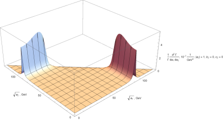
a
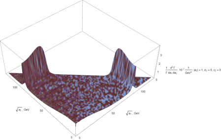
b

Figure 3: The distribution $\frac{1}{\Gamma}\frac{d^{2}\Gamma}{da_{1}da_{2}}$ (in units of $10^{-7}\,{\rm GeV}^{-4}$) in the SM for the decays $h\to Z_{1}^{*}Z_{2}^{*}\to f_{1}\bar{f}_{1}f_{2}\bar{f}_{2}$ with $f_{1}\neq f_{2}$ (a) and for the decays $h\to Z_{1}^{*}Z_{2}^{*}\to 4l$ with $l=e,\mu,\tau$ (b).

Figure 4 shows the distributions $\frac{1}{\Gamma}\frac{d\Gamma}{da}$, $\frac{1}{\sin\theta}\frac{1}{\Gamma}\frac{d\Gamma}{d\theta}$, and $\frac{1}{\Gamma}\frac{d\Gamma}{d\phi}$ for the decay to non-identical leptons and the decay to identical ones. The definitions and explicit formulas for the differential widths $\frac{d\Gamma}{da}$ and $\frac{d\Gamma}{d\theta}$ are given in C (see Eqs. (40), (48), (49), and (54)).

a

b

Figure 4: The distributions $\frac{1}{\Gamma}\frac{d\Gamma}{da}$, $\frac{1}{\sin\theta}\frac{1}{\Gamma}\frac{d\Gamma}{d\theta}$, and $\frac{1}{\Gamma}\frac{d\Gamma}{d\phi}$ for the decays $h\to Z_{1}^{*}Z_{2}^{*}\to l_{1}^{-}l_{1}^{+}l_{2}^{-}l_{2}^{+}$; $l_{j}=e,\mu,\tau$ in the cases $l_{1}\neq l_{2}$ (a) and $l_{1}=l_{2}$ (b). The solid, dashed, dot-dashed, and dotted lines correspond to sets (3) respectively.

The distributions in Fig. 4 are presented at the following four sets of values of the couplings $a_{Z}$, $b_{Z}$, and $c_{Z}$:

$$|a_{Z}|=1,\;b_{Z}=0,\;c_{Z}=0,$$

$$a_{Z}=1,\;b_{Z}=0,\;c_{Z}=0.5,$$

$$a_{Z}=1,\;b_{Z}=0,\;c_{Z}=0.5\,i,$$

$$a_{Z}=1,\;b_{Z}=-0.5,\;c_{Z}=0.$$ (14)

In Ref. 32 sets (3) are shown to be consistent with the available LHC data and are chosen for an analysis of some observables sensitive to the $hZZ$ couplings.

The dependences in the upper plot of Fig. 4a are calculated using Eq. (A.2) from Ref. 32 and Eq. (B) from this paper. To obtain the lines shown in the two other plots of Fig. 4a, we first integrate Eq. (A) with a MC method and obtain four sets of dots. Then we fit each set by means of the method of least squares. In order not to clutter the plots, we show only the fitting lines and do not present the dots.

To derive the distributions $\frac{1}{\Gamma}\frac{d\Gamma}{da}$, $\frac{1}{\sin\theta}\frac{1}{\Gamma}\frac{d\Gamma}{d\theta}$, and $\frac{1}{\Gamma}\frac{d\Gamma}{d\phi}$ for the decay into identical leptons, we integrate Eq. (A) with a MC method and obtain sets of dots. The lines in the upper plot of Fig. 4b consist of cubic parabolas joining the neighboring dots, since we have not been able to properly fit the dots of this plot with the method of least squares. The lines in the two other plots of Fig. 4b are least-squares fits to the corresponding dots. As in Fig. 4a, the dots are not shown to avoid cluttering of the plots.

The relative uncertainties of the dots used for plotting the dependences in Fig. 4 are estimated during the MC integration. For any of the plotted distributions, these uncertainties turned out to be virtually the same for each dot and each set (3). Thus, they depend only on what distribution we consider. One standard deviation of a fitting line has been estimated using Eq. (10) from Ref. 46. The uncertainties and one standard deviations for the distributions of the decays into non-identical or identical leptons are presented in Table 3. The estimates shown in Table 3 do not account for the uncertainties of the constants listed in Table 3.

The relative uncertainties $\delta_{d}$ of the dots and the standard deviations $\sigma_{f}$ of the fitting lines for some distributions of the decay $h\to Z_{1}^{*}Z_{2}^{*}\to l_{1}^{-}l_{1}^{+}l_{2}^{-}l_{2}^{+}$ ($l_{j}=e,\mu,\tau$). Distribution non-identical leptons identical leptons $\delta_{d}$ $\sigma_{f}$ $\delta_{d}$ $\sigma_{f}$ $\frac{1}{\Gamma}\frac{d\Gamma}{da}$ – – 1.8 % – $\frac{1}{\sin\theta}\frac{1}{\Gamma}\frac{d\Gamma}{d\theta}$ 2 % $1.2\cdot 10^{-3}$ 1.6 % $2.4\cdot 10^{-3}$ $\frac{1}{\Gamma}\frac{d\Gamma}{d\phi}$ 2 % $5\cdot 10^{-4}$ 2 % $7\cdot 10^{-4}$

We note that according to Fig. 3 in Ref. 47, the distinctions between the SM distributions $\frac{1}{\sin\theta}\frac{1}{\Gamma}\frac{d\Gamma}{d\theta}$ and $\frac{1}{\Gamma}\frac{d\Gamma}{d\phi}$ for the decay into non-identical leptons and those for the decay into identical ones are not as significant as these distinctions according to Fig. 4 in the present article. There can be a few sources of the differences with Fig. 3 in Ref. 47:

i) we consider the tree-level decays $h\to Z_{1}^{*}Z_{2}^{*}\to l_{1}^{-}l_{1}^{+}l_{2}^{-}l_{2}^{+}$ while the dependences in Fig. 3 of Ref. 47 are calculated at next-to-leading order (NLO) accuracy;

ii) we have numerically integrated Eq. (8) from Ref. 32 and Eqs. (A) and (A) from the present article, while MC integration with PROPHECY4f was used in Ref. 47;

iii) our definitions of the $Z$ boson couplings to fermions $a_{f}$ and $v_{f}$ and the asymmetry parameter $A_{f}$ are given in A. These definitions yield $a_{l}=-0.5$, $v_{l}=-0.054$, and $A_{l}=0.214$ ($l=e,\mu,\tau$). However, experimental values of these parameters are different. For instance, for the electron $a_{e}^{exp}=-0.50123$, $v_{e}^{exp}=-0.03783$, and $A_{e}^{exp}=0.1515$ (see Ref. 45). The difference in $a_{e}$, $v_{e}$, and $A_{e}$ causes a certain distinction in the shapes of the distributions $\frac{1}{\sin\theta}\frac{1}{\Gamma}\frac{d\Gamma}{d\theta}$ and $\frac{1}{\Gamma}\frac{d\Gamma}{d\phi}$;

iv) in the present article non-histrogram distributions are plotted.

The dependences plotted in Fig. 4 almost coincide at all four sets (3). For this reason, we can get significant constraints on $a_{Z}$, $b_{Z}$, and $c_{Z}$ via measurement of the distributions $\frac{1}{\Gamma}\frac{d\Gamma}{da}$, $\frac{1}{\sin\theta}\frac{1}{\Gamma}\frac{d\Gamma}{d\theta}$, and $\frac{1}{\Gamma}\frac{d\Gamma}{d\phi}$ only if these distributions are measured at very high precision. That is why in order to constrain the $hZZ$ couplings, we should try to define observables sensitive to these couplings, like it is done in Ref. 32 for decay (2).

The distinctions between the distributions $\frac{1}{\Gamma}\frac{d\Gamma}{da}$ for the decay into non-identical leptons (Fig. 4a) and those for identical leptons (Fig. 4b) are due to greater values of the SM distribution $\frac{1}{\Gamma}\frac{d^{2}\Gamma}{da_{1}da_{2}}$ on the plateau for the decay $h\to Z_{1}^{*}Z_{2}^{*}\to 4l$ and smaller values of this distribution at the peaks $\sqrt{a_{1}}=m_{Z}$ and $\sqrt{a_{2}}=m_{Z}$ (see Fig. 3). However, these distinctions are insubstantial.

The dissimilarity between the functions $\frac{1}{\sin\theta}\frac{1}{\Gamma}\frac{d\Gamma}{d\theta}$ and $\frac{1}{\Gamma}\frac{d\Gamma}{d\phi}$ in Figs. 4a and 4b is much more appreciable. The global maximum of $\frac{1}{\sin\theta}\frac{1}{\Gamma}\frac{d\Gamma}{d\theta}$ at $\theta=\pi/2$ in Fig. 4a becomes a local minimum in Fig. 4b, and the values near the points $\theta=0$ and $\theta=\pi$ increase. Analogous distinctions take place between the dependences of $\frac{1}{\Gamma}\frac{d\Gamma}{d\phi}$ in Figs. 4a and 4b.

4 Comparison with experimental data

4.1 ATLAS and CMS results

In Ref. 30 the ATLAS collaboration presents experimental distributions of the decay $h\to Z_{1}^{*}Z_{2}^{*}\to 4\ell$ and corresponding distributions derived with MC simulations in the SM. We take the same kinematic limitations and the bin widths as ATLAS and use Eqs. (A) and (A) to derive the SM histogram distributions of the decay $h\to Z_{1}^{*}Z_{2}^{*}\to 4\ell$ which appear in Ref. 30. Comparison of our distributions with the ATLAS experimental and theoretical ones will determine the usefulness of Eq. (A).

CMS has shown experimental distributions for the decay $h\to VV\to 4\ell$ ($VV=ZZ$, $Z\gamma$, $\gamma\gamma$) and corresponding MC simulations in the SM in Ref. 31. Taking the same kinematic limitations and the same bin widths as CMS, we integrate Eqs. (A) and (A) in the SM to obtain distributions for the decay $h\to Z_{1}^{*}Z_{2}^{*}\to 4\ell$.

We introduce the four following variables: $m_{12}$ ($m_{34}$) is the invariant mass of the $Z$ boson which is produced in a decay $h\to Z_{1}^{*}Z_{2}^{*}\to 4\ell$ and whose mass is closest to (most distant from) $m_{Z}$, $\theta_{1}^{\prime}$ ($\theta_{2}^{\prime}$) is the polar angle of the fermion whose parent $Z$ boson has the invariant mass closest to (most distant from) $m_{Z}$. From the definitions of $m_{12}$ and $m_{34}$ it follows that

$$|m_{12}-m_{Z}|<|m_{34}-m_{Z}|.$$ (15)

However, since $m_{h}<2\,m_{Z}$, the quantity $m_{12}$ ($m_{34}$) can be equivalently defined as the invariant mass of the heaviest (lightest) $Z$ boson produced in a decay $h\to Z_{1}^{*}Z_{2}^{*}\to 4\ell$ ($m_{12}>m_{34}$).

In Ref. 30 ATLAS shows distributions of $m_{12}$, $m_{34}$, $\cos\theta_{1}^{\prime}$, and $\phi$ (a distribution of $\cos\theta_{2}^{\prime}$ is not presented). ATLAS selects events $h\to Z_{1}^{*}Z_{2}^{*}\to 4\ell$ wherein

$$m_{12}\in(50~{}{\rm GeV},106~{}{\rm GeV}),\qquad m_{34}\in(12~{}{\rm GeV},115~{}{\rm GeV}),$$

$$\eta_{e}\in(-2.47,2.47),\qquad\eta_{\mu}\in(-2.7,2.7).$$ (16)

Here $\eta_{e}$ ($\eta_{\mu}$) is the pseudorapidity of the electron (muon):

$$\eta_{i}(\theta_{i})\equiv-\ln\tan\frac{\theta_{i}}{2},\qquad i=e,\mu,$$ (17)

where $\theta_{e}$ ($\theta_{\mu}$) is the polar angle of the electron (muon).

CMS paper [31] presents distributions of $m_{12}$, $m_{34}$, $\cos\theta_{1}^{\prime}$, $\cos\theta_{2}^{\prime}$, and $\phi$ for the decay $h\to VV\to 4\ell$ with

$$m_{12}\in(40~{}{\rm GeV},120~{}{\rm GeV}),\qquad m_{34}\in(12~{}{\rm GeV},120~{}{\rm GeV}),$$

$$\eta_{e}\in(-2.5,2.5),\qquad\eta_{\mu}\in(-2.4,2.4).$$ (18)

Constraints (4.1) and (4.1) determine the fractions of decays selected by ATLAS or CMS in the corresponding decay modes. These fractions are given by the left-hand sides of Eqs. (55) and (63). We have calculated the corresponding percentages in the SM (see Table 4.1).

The SM percentages $P_{SM}$ of decays selected by the CMS and ATLAS collaborations (see Eqs. (4.1) and (4.1)), for various decay modes. Decay mode $P_{SM}$ CMS ATLAS $h\to Z_{1}^{*}Z_{2}^{*}\to 4e$ 84.6 % 75.6 % $h\to Z_{1}^{*}Z_{2}^{*}\to 4\mu$ 84.1 % 76.4 % $h\to Z_{1}^{*}Z_{2}^{*}\to 2e2\mu$ 86.5 % 85.1 % $h\to Z_{1}^{*}Z_{2}^{*}\to 4\ell$ 85.5 % 81.1 %

4.2 A discussion of plots

Integrating Eq. (D) with a MC method, we derive some SM histogram distributions of the decay $h\to Z_{1}^{*}Z_{2}^{*}\to 4\ell$ (see the blue lines in Figs. 5 and 6). The bin widths in Fig. 5 are taken from Ref. 30 while those in Fig. 6 are taken from Ref. 31.

Figure 5: The numbers of events $h\to Z_{1}^{*}Z_{2}^{*}\to 4\ell$ in bins of $m_{12}$, $m_{34}$, $\cos\theta_{1}^{\prime}$, $\cos\theta_{2}^{\prime}$, and $\phi$ according to our calculations in the SM (solid lines), the ATLAS (Ref. 30) MC simulations in the SM (dashed lines), and the ATLAS experimental data in Ref. 30 (points with error bars). In our computations the total number of events $h\to Z_{1}^{*}Z_{2}^{*}\to 4\ell$ is chosen to be 45. Both our calculations and the ATLAS MC simulations are carried out for ATLAS limitations (4.1).

Figure 6: The numbers of events $h\to Z_{1}^{*}Z_{2}^{*}\to 4\ell$ in bins of $m_{12}$, $m_{34}$, $\cos\theta_{1}^{\prime}$, $\cos\theta_{2}^{\prime}$, and $\phi$ according to our calculations in the SM. The total number of events $h\to Z_{1}^{*}Z_{2}^{*}\to 4\ell$ is chosen to be 50. Our computations are performed for CMS limitations (4.1).

ATLAS reports about 45 events $h\to Z_{1}^{*}Z_{2}^{*}\to 4\ell$ with $m_{4\ell}\in(115\,{\rm GeV},130\,{\rm GeV})$ ($m_{4\ell}$ is the invariant mass of the 4 final leptons) in Ref. 30 (see Table 3 there). For this reason, we have calculated our distributions shown in Fig. 5, setting $N_{4\ell}^{{\rm ATLAS}}=45$ in Eq. (D).

It is of interest to sum up the numbers of events over all the bins for each plot in Fig. 5 (see Table 4.2).

The sums over all the bins for each plot in Fig. 5 ($\Sigma_{m_{12}}$, $\Sigma_{m_{34}}$,$\Sigma_{\cos\theta_{1}^{\prime}}$, $\Sigma_{\cos\theta_{2}^{\prime}}$, and $\Sigma_{\phi}$) for the ATLAS experimental data, for the ATLAS MC simulated distributions, and for our distributions. ATLAS exp. data ATLAS MC simulated distributions Our distributions $\Sigma_{m_{12}}$ 45 40.31 46.16 $\Sigma_{m_{34}}$ 41 41.14 43.31 $\Sigma_{\cos\theta_{1}^{\prime}}$ 45 40.81 47.24 $\Sigma_{\cos\theta_{2}^{\prime}}$ n/a n/a 46.63 $\Sigma_{\phi}$ 45 41.09 46.30

The total number of the events in the ATLAS experimental distribution of $m_{34}$ is 41. That is why 4 events measured by ATLAS are not presented in this distribution. Therefore, in these events $m_{34}\in(12\,{\rm GeV},15\,{\rm GeV})$ (see ATLAS limitations (4.1) and Fig. 5). The bin sum 41.14 for the ATLAS simulated distribution of $m_{34}$ is notably closer to 41 than the bin sum 43.31 for our distribution of $m_{34}$.

For the ATLAS simulated distributions of $m_{12}$, $\cos\theta_{1}^{\prime}$, and $\cos\theta_{2}^{\prime}$ the bin sums are also close to 41. We take $N_{4\ell}^{{\rm ATLAS}}=45$ for all our distributions, and our bin sums $\Sigma_{m_{12}}$, $\Sigma_{\cos\theta_{1}^{\prime}}$, and $\Sigma_{\phi}$ are significantly closer to 45 than those for the ATLAS simulated distributions.

On the other hand, the ATLAS simulations take into account that for the 45 measured events $m_{4\ell}$ varies from 115 GeV to 130 GeV while we use Eqs. (A) and (A), which are derived for the case $m_{4\ell}=m_{h}$.

Summarizing the comparison with the ATLAS results, we note that our distributions are derived by integration of analytical formulas obtained for $m_{4\ell}=m_{h}$ and we have thoroughly chosen the total number of events. ATLAS has used MC simulations and has accounted for the fact that for the measured events $m_{4\ell}$ varies from 115 GeV to 130 GeV. Both techniques have advantages and disadvantages, and therefore it is not surprising that the ATLAS simulated distributions and our distributions somewhat differ but are equally close to the ATLAS experimental distributions (see Fig. 5). In addition, we present our distribution of $\cos\theta_{2}^{\prime}$.

In Ref. 31 CMS reports about 50 observed events $h\to VV\to 4\ell$ with $m_{4\ell}\in(105.6\,{\rm GeV},140.6\,{\rm GeV})$ (see Table 3 there). In view of this, in order to calculate distributions for the CMS limitations (4.1), we choose $N_{4\ell}^{{\rm CMS}}=50$ in Eq. (D). The accuracy of our distributions shown in Fig. 6 can be characterized by the sums over all the bins for each plot (see Table 4.2). The plots in Fig. 6 are smoother than those in Fig. 5 due to their smaller bin widths.

The sums over all the bins for each plot in Fig. 6. Our distributions $\Sigma_{m_{12}}$ 51.30 $\Sigma_{m_{34}}$ 55.91 $\Sigma_{\cos\theta_{1}^{\prime}}$ 52.14 $\Sigma_{\cos\theta_{2}^{\prime}}$ 52.03 $\Sigma_{\phi}$ 51.34

5 Conclusions

In this paper, we have considered the decay of a neutral particle $X$ with zero spin and arbitrary $CP$ parity into two off-mass-shell $Z$ bosons ($Z_{1}^{*}$ and $Z_{2}^{*}$) each of which decays to identical fermion-antifermion pairs ($f\bar{f}$): $X\to Z_{1}^{*}Z_{2}^{*}\to f\bar{f}f\bar{f}$. Analytical formulas for the fully differential width of the decay in question and for the fully differential width of the decay $h\to Z_{1}^{*}Z_{2}^{*}\to 4\ell$ are derived (see Eqs. (A) and (D)). Moreover, we present an exact formula for the differential width $\frac{d\Gamma}{da}$ of a decay $X\to Z_{1}^{*}Z_{2}^{*}\to f_{1}\bar{f}_{1}f_{2}\bar{f}_{2}$ with $f_{1}\neq f_{2}$ (see Eq. (B)).

Integrating Eq. (A) with a MC method, we have obtained some non-histogram distributions for any decay $h\to Z_{1}^{*}Z_{2}^{*}\to l_{1}^{-}l_{1}^{+}l_{2}^{-}l_{2}^{+}$ ($l_{j}=e,\mu,\tau$) with $l_{1}=l_{2}$. These distributions are compared to those for the decay $h\to Z_{1}^{*}Z_{2}^{*}\to l_{1}^{-}l_{1}^{+}l_{2}^{-}l_{2}^{+}$ with $l_{1}\neq l_{2}$ (see Figs. 3 and 4). The comparison has revealed significant distinctions between the distributions for the case $l_{1}=l_{2}$ and the corresponding ones for $l_{1}\neq l_{2}$. However, in the SM some of these distinctions may be less noticeable, as Figure 3 in Ref. 47 presents. The difference between the results of Ref. 47 and our ones can arise due to several reasons discussed in Section 3. The dependences shown in Fig. 4 are calculated at four possible sets (3) of values of the $hZZ$ couplings $a_{Z}$, $b_{Z}$, and $c_{Z}$. At all the four sets these distributions almost coincide. Therefore their measurement can yield notable constraints on $a_{Z}$, $b_{Z}$, and $c_{Z}$ only if the distributions are measured at very high precision.

In order to determine the usefulness of Eq. (A), we have computed some SM histogram distributions of the decay $h\to Z_{1}^{*}Z_{2}^{*}\to 4\ell$ by means of integration of Eq. (D). The distributions are calculated for ATLAS kinematical limitations (4.1) and for CMS ones (4.1).

We have compared our distributions with the ATLAS experimental ones and the ATLAS MC simulated ones (see Ref. 30). The way our distributions are derived is almost purely analytical — its only numerical part is integration of Eq. (D). Besides, we have chosen the total number of events more accurately than ATLAS during its simulations. However, our calculation does not allow for the fact that the invariant mass of $4\ell$ may differ from $m_{h}$ while this fact is taken into account in the ATLAS simulations. The pros and cons of our technique and the ATLAS simulations make our distributions and the ATLAS simulated ones somewhat different but equally close to the ATLAS experimental data.

We have also presented our distributions of $m_{12}$, $m_{34}$, $\cos\theta_{1}^{\prime}$, $\cos\theta_{2}^{\prime}$, and $\phi$ for the kinematic conditions specific for CMS.

In summary, various distributions of the decays $X\to Z_{1}^{*}Z_{2}^{*}\to f\bar{f}f\bar{f}$ or $h\to Z_{1}^{*}Z_{2}^{*}\to 4\ell$ have been obtained with a rather simple integration of Eqs. (A) and (D) respectively. This way of calculation gives an alternative to more traditional MC simulation.

Appendix A The fully differential width of the decay $X\to Z_{1}^{*}Z_{2}^{*}\to f\bar{f}f\bar{f}$

The fully differential width of decay (3) is

$$\frac{d^{5}\Gamma}{da_{1}da_{2}d\theta_{1}d\theta_{2}d\varphi}= \frac{1}{4}\Biggl{[}\left.\frac{d^{5}\Gamma_{f_{1}\neq f_{2}}}{da_{1}da_{2}d\theta_{1}d\theta_{2}d\varphi}\right|_{f_{1}=f_{2}=f}+\frac{\sqrt{2}G_{F}^{3}m_{Z}^{8}}{(4\pi)^{6}m_{X}^{3}}\frac{k\sqrt{\tilde{a}_{1}\tilde{a}_{2}}}{D(\tilde{a}_{1})D(\tilde{a}_{2})}(a_{f}^{2}+v_{f}^{2})^{2}\sin\theta_{1}\sin\theta_{2}$$

$$\times\biggl{\{}\sqrt{\tilde{a}_{1}\tilde{a}_{2}}\Bigl{\{}\left((1+\bar{\alpha}_{3}^{2})(1+\bar{\beta}_{3}^{2})+4A_{f}^{2}\bar{\alpha}_{3}\bar{\beta}_{3}\right)(|\tilde{A}_{\parallel}|^{2}+|\tilde{A}_{\perp}|^{2})+4(1-\bar{\alpha}_{3}^{2})(1-\bar{\beta}_{3}^{2})|\tilde{A}_{0}|^{2}$$

$$-4A_{f}\left(\bar{\alpha}_{3}(1+\bar{\beta}_{3}^{2})+\bar{\beta}_{3}(1+\bar{\alpha}_{3}^{2})\right){\rm Re}(\tilde{A}_{\parallel}^{*}\tilde{A}_{\perp})+4\sqrt{2}\Bigl{(}(A_{f}^{2}+\bar{\alpha}_{3}\bar{\beta}_{3})\bigl{(}{\rm Re}\eta_{-}{\rm Re}(\tilde{A}_{0}^{*}\tilde{A}_{\parallel})$$

$$+{\rm Im}\eta_{-}{\rm Im}(\tilde{A}_{0}^{*}\tilde{A}_{\perp})\bigr{)}-A_{f}(\bar{\alpha}_{3}+\bar{\beta}_{3})\bigl{(}{\rm Re}\eta_{-}{\rm Re}(\tilde{A}_{0}^{*}\tilde{A}_{\perp})+{\rm Im}\eta_{-}{\rm Im}(\tilde{A}_{0}^{*}\tilde{A}_{\parallel})\bigr{)}\Bigr{)}$$

$$+{\rm Re}\eta_{-}^{2}(|\tilde{A}_{\parallel}|^{2}-|\tilde{A}_{\perp}|^{2})+2\,{\rm Im}\eta_{-}^{2}{\rm Im}(\tilde{A}_{\parallel}^{*}\tilde{A}_{\perp})\Bigl{\}}-\frac{\sqrt{a_{1}a_{2}}}{D(a_{1})D(a_{2})}$$

$$\times{\rm Re}\Bigl{\{}(a_{1}-m_{Z}^{2}+im_{Z}\Gamma_{Z})(a_{2}-m_{Z}^{2}+im_{Z}\Gamma_{Z})(\tilde{a}_{1}-m_{Z}^{2}-im_{Z}\Gamma_{Z})(\tilde{a}_{2}-m_{Z}^{2}-im_{Z}\Gamma_{Z})$$

$$\times\Bigl{(}\bigl{(}(r_{\alpha\beta}+\frac{1}{r_{\alpha\beta}})({\rm Re}\eta_{-}\tilde{A}_{\parallel}-i{\rm Im}\eta_{-}\tilde{A}_{\perp})+2\sqrt{2(1-\bar{\alpha}_{3}^{2})(1-\bar{\beta}_{3}^{2})}\tilde{A}_{0}\bigr{)}$$

$$\times\bigl{(}((1+A_{f}^{2})\cos\phi(1+\cos\theta_{1}\cos\theta_{2})+i\cdot 2A_{f}\sin\phi(\cos\theta_{1}+\cos\theta_{2}))A_{\parallel}^{*}$$

$$-(2A_{f}\cos\phi(\cos\theta_{1}+\cos\theta_{2})+i(1+A_{f}^{2})\sin\phi(1+\cos\theta_{1}\cos\theta_{2}))A_{\perp}^{*}$$

$$+\sqrt{2}(1+A_{f}^{2})\sin\theta_{1}\sin\theta_{2}A_{0}^{*}\bigr{)}+(r_{\alpha\beta}-\frac{1}{r_{\alpha\beta}})(i{\rm Im}\eta_{-}\tilde{A}_{\parallel}-{\rm Re}\eta_{-}\tilde{A}_{\perp})$$

$$\times\bigl{(}(2A_{f}\cos\phi(1+\cos\theta_{1}\cos\theta_{2})+i(1+A_{f}^{2})\sin\phi(\cos\theta_{1}+\cos\theta_{2}))A_{\parallel}^{*}$$

$$-((1+A_{f}^{2})\cos\phi(\cos\theta_{1}+\cos\theta_{2})+i\cdot 2A_{f}\sin\phi(1+\cos\theta_{1}\cos\theta_{2}))A_{\perp}^{*}$$

$$+\sqrt{2}\cdot 2A_{f}\sin\theta_{1}\sin\theta_{2}A_{0}^{*}\bigr{)}\Bigr{)}\Bigr{\}}\biggr{\}}\Biggr{]},$$ (19)

where

$$\frac{d^{5}\Gamma_{f_{1}\neq f_{2}}}{da_{1}da_{2}d\theta_{1}d\theta_{2}d\varphi}= \frac{\sqrt{2}G_{F}^{3}m_{Z}^{8}}{(4\pi)^{6}m_{X}^{3}}(a_{f_{1}}^{2}+v_{f_{1}}^{2})(a_{f_{2}}^{2}+v_{f_{2}}^{2})\frac{ka_{1}a_{2}}{D(a_{1})D(a_{2})}$$

$$\times\sin\theta_{1}\sin\theta_{2}[(|A_{\parallel}|^{2}+|A_{\perp}|^{2})\left((1+\cos^{2}\theta_{1})(1+\cos^{2}\theta_{2})+4A_{f_{1}}A_{f_{2}}\cos\theta_{1}\cos\theta_{2}\right)$$

$$+4|A_{0}|^{2}\sin^{2}\theta_{1}\sin^{2}\theta_{2}-4\,{\rm Re}(A_{\parallel}^{*}A_{\perp})(A_{f_{1}}\cos\theta_{1}(1+\cos^{2}\theta_{2})+A_{f_{2}}\cos\theta_{2}(1+\cos^{2}\theta_{1}))$$

$$+4\sqrt{2}\sin\theta_{1}\sin\theta_{2}(({\rm Re}(A_{0}^{*}A_{\parallel})\cos\phi-{\rm Im}(A_{0}^{*}A_{\perp})\sin\phi)(A_{f_{1}}A_{f_{2}}+\cos\theta_{1}\cos\theta_{2})$$

$$-({\rm Re}(A_{0}^{*}A_{\perp})\cos\phi-{\rm Im}(A_{0}^{*}A_{\parallel})\sin\phi)(A_{f_{1}}\cos\theta_{2}+A_{f_{2}}\cos\theta_{1}))$$

$$+\sin^{2}\theta_{1}\sin^{2}\theta_{2}((|A_{\parallel}|^{2}-|A_{\perp}|^{2})\cos 2\phi-2\,{\rm Im}(A_{\parallel}^{*}A_{\perp})\sin 2\phi)]$$ (20)

is the fully differential width of decay (2) (see Eq. (5) in Ref. 32), $a_{f}$ is the weak isospin projection of the fermion $f$, $v_{f}\equiv a_{f}-2\frac{q_{f}}{e}\sin^{2}\theta_{W}$, $q_{f}$ is the electric charge of $f$, $e$ is the electric charge of the positron, $\theta_{W}$ is the weak mixing angle, $D(x)\equiv(x-m_{Z}^{2})^{2}+(m_{Z}\Gamma_{Z})^{2}$,

$$A_{\pm}\equiv\frac{A_{X\rightarrow Z_{1}^{*}Z_{2}^{*}}(p_{1},p_{2},\pm 1,\pm 1)}{g_{Z}},\qquad A_{0}\equiv\frac{A_{X\rightarrow Z_{1}^{*}Z_{2}^{*}}(p_{1},p_{2},0,0)}{g_{Z}},$$ (21)

$$A_{\parallel}\equiv\frac{\tilde{A}_{+}+\tilde{A}_{-}}{\sqrt{2}}=\sqrt{2}a_{Z}(a_{1},a_{2}),\qquad A_{\perp}\equiv\frac{\tilde{A}_{+}-\tilde{A}_{-}}{\sqrt{2}}=\sqrt{2}\frac{k}{m_{X}^{2}}c_{Z}(a_{1},a_{2}),$$ (22)

$$A_{f}=\frac{2a_{f}v_{f}}{a_{f}^{2}+v_{f}^{2}},$$ (23)

$\bar{\alpha}_{i}\equiv\frac{\alpha_{i}}{|\boldsymbol{\alpha}|}~{}(i=1,2,3)$, $\boldsymbol{\alpha}$ is the momentum of the fermion $f_{1}$ in the center-of-momentum frame of the particles $f_{1}$ and $\bar{f}_{2}$,

$$\boldsymbol{\alpha}= \mathbf{e}_{x}\frac{\sqrt{a_{1}}(2E_{2}^{\prime}+\sqrt{\tilde{a}_{1}})\sin\theta_{1}\cos\phi_{1}+\sqrt{a_{2}}(2E_{1}+\sqrt{\tilde{a}_{1}})\sin\theta_{2}\cos\phi_{2}}{4(E_{1}+E_{2}^{\prime}+\sqrt{\tilde{a}_{1}})}$$

$$+\mathbf{e}_{y}\frac{\sqrt{a_{1}}(2E_{2}^{\prime}+\sqrt{\tilde{a}_{1}})\sin\theta_{1}\sin\phi_{1}-\sqrt{a_{2}}(2E_{1}+\sqrt{\tilde{a}_{1}})\sin\theta_{2}\sin\phi_{2}}{4(E_{1}+E_{2}^{\prime}+\sqrt{\tilde{a}_{1}})}+\frac{\bar{\mathbf{p}}_{1}}{8(E_{1}+E_{2}^{\prime}+\sqrt{\tilde{a}_{1}})}$$

$$\times\Bigl{(}(m_{X}^{2}-a_{1}-a_{2})(\cos\theta_{1}-\cos\theta_{2})+k(1-\cos\theta_{1}\cos\theta_{2})$$

$$+\frac{\sqrt{\tilde{a}_{1}}}{m_{X}}(2k+(m_{X}^{2}+a_{1}-a_{2})\cos\theta_{1}-(m_{X}^{2}+a_{2}-a_{1})\cos\theta_{2})\Bigr{)},$$ (24)

$$|\boldsymbol{\alpha}|= \frac{\sqrt{\tilde{a}_{1}}}{2},$$ (25)

$\bar{\mathbf{p}}_{1}\equiv\frac{\mathbf{p}_{1}}{|\mathbf{p}_{1}|}$, $\mathbf{e}_{x}$ and $\mathbf{e}_{y}$ are any unit and mutually orthogonal vectors such that $\mathbf{e}_{x}\times\mathbf{e}_{y}=\bar{\mathbf{p}}_{1}$,

$$E_{1}\equiv k_{1}^{0}=\frac{m_{X}^{2}+a_{1}-a_{2}+k\cos\theta_{1}}{4m_{X}},\qquad E_{1}^{\prime}\equiv k_{1}^{\prime 0}=\frac{m_{X}^{2}+a_{1}-a_{2}-k\cos\theta_{1}}{4m_{X}}$$

$$E_{2}\equiv k_{2}^{0}=\frac{m_{X}^{2}+a_{2}-a_{1}+k\cos\theta_{2}}{4m_{X}},\qquad E_{2}^{\prime}\equiv k_{2}^{\prime 0}=\frac{m_{X}^{2}+a_{2}-a_{1}-k\cos\theta_{2}}{4m_{X}},$$ (26)

$\phi_{1}$ is the azimuthal angle of the $f_{1}$ momentum in the $Z_{1}^{*}$ rest frame formed by the vectors ($\mathbf{e}_{x}$, $\mathbf{e}_{y}$, $\bar{\mathbf{p}}_{1}$), $\phi_{2}$ is the azimuthal angle of the $f_{2}$ momentum in the $Z_{2}^{*}$ rest frame formed by the vectors ($\mathbf{e}_{x}$, $-\mathbf{e}_{y}$, $-\bar{\mathbf{p}}_{1}$),

$$\alpha_{1}\equiv\boldsymbol{\alpha}\cdot\mathbf{e}_{x},~{}~{}\alpha_{2}\equiv\boldsymbol{\alpha}\cdot\mathbf{e}_{y},~{}~{}\alpha_{3}\equiv\boldsymbol{\alpha}\cdot\bar{\mathbf{p}}_{1},$$ (27)

$\bar{\beta}_{i}\equiv\frac{\beta_{i}}{|\boldsymbol{\beta}|}~{}(i=1,2,3)$, $\boldsymbol{\beta}$ is the momentum of the fermion $f_{2}$ in the center-of-momentum frame of the particles $f_{2}$ and $\bar{f}_{1}$,

$$\boldsymbol{\beta} =\boldsymbol{\alpha}|_{\begin{subarray}{c}a_{1}\leftrightarrow a_{2},\theta_{1}\leftrightarrow\theta_{2},\phi_{1}\leftrightarrow\phi_{2}\\ \mathbf{e}_{y}\to-\mathbf{e}_{y},\bar{\mathbf{p}}_{1}\to-\bar{\mathbf{p}}_{1}\end{subarray}}=\boldsymbol{\alpha}|_{k\rightarrow-k}$$

$$=\mathbf{e}_{x}\frac{\sqrt{a_{1}}(2E_{2}+\sqrt{\tilde{a}_{2}})\sin\theta_{1}\cos\phi_{1}+\sqrt{a_{2}}(2E_{1}^{\prime}+\sqrt{\tilde{a}_{2}})\sin\theta_{2}\cos\phi_{2}}{4(E_{2}+E_{1}^{\prime}+\sqrt{\tilde{a}_{2}})}$$

$$+\mathbf{e}_{y}\frac{\sqrt{a_{1}}(2E_{2}+\sqrt{\tilde{a}_{2}})\sin\theta_{1}\sin\phi_{1}-\sqrt{a_{2}}(2E_{1}^{\prime}+\sqrt{\tilde{a}_{2}})\sin\theta_{2}\sin\phi_{2}}{4(E_{2}+E_{1}^{\prime}+\sqrt{\tilde{a}_{2}})}+\frac{\bar{\mathbf{p}}_{1}}{8(E_{2}+E_{1}^{\prime}+\sqrt{\tilde{a}_{2}})}$$

$$\times\Bigl{(}(m_{X}^{2}-a_{1}-a_{2})(\cos\theta_{1}-\cos\theta_{2})-k(1-\cos\theta_{1}\cos\theta_{2})$$

$$+\frac{\sqrt{\tilde{a}_{2}}}{m_{X}}(-2k+(m_{X}^{2}+a_{1}-a_{2})\cos\theta_{1}-(m_{X}^{2}+a_{2}-a_{1})\cos\theta_{2})\Bigr{)},$$ (28)

$$|\boldsymbol{\beta}| =\frac{\sqrt{\tilde{a}_{2}}}{2},$$ (29)

$$\beta_{1}\equiv\boldsymbol{\beta}\cdot\mathbf{e}_{x},~{}~{}\beta_{2}\equiv\boldsymbol{\beta}\cdot(-\mathbf{e}_{y}),~{}~{}\beta_{3}\equiv\boldsymbol{\beta}\cdot(-\bar{\mathbf{p}}_{1}),$$ (30)

$$\tilde{A}_{\pm}\equiv\frac{A_{X\rightarrow Z_{1}^{*}Z_{2}^{*}}(\tilde{p}_{1},\tilde{p}_{2},\pm 1,\pm 1)}{g_{Z}},\qquad\tilde{A}_{0}\equiv\frac{A_{X\rightarrow Z_{1}^{*}Z_{2}^{*}}(\tilde{p}_{1},\tilde{p}_{2},0,0)}{g_{Z}},$$ (31)

$$\tilde{A}_{\parallel}\equiv\frac{\tilde{A}_{+}+\tilde{A}_{-}}{\sqrt{2}}=\sqrt{2}a_{Z}(\tilde{a}_{1},\tilde{a}_{2}),\qquad\tilde{A}_{\perp}\equiv\frac{\tilde{A}_{+}-\tilde{A}_{-}}{\sqrt{2}}=\frac{2\sqrt{2}}{m_{X}}|\mathbf{k}_{1}+\mathbf{k}_{2}^{\prime}|c_{Z}(\tilde{a}_{1},\tilde{a}_{2}),$$ (32)

$$\eta_{-} \equiv(\bar{\alpha}_{1}-i\bar{\alpha}_{2})(\bar{\beta}_{1}-i\bar{\beta}_{2})$$

$$=\frac{1}{4\sqrt{\tilde{a}_{1}\tilde{a}_{2}}(E_{1}+E_{2}^{\prime}+\sqrt{\tilde{a}_{1}})(E_{2}+E_{1}^{\prime}+\sqrt{\tilde{a}_{2}})}\Biggl{(}a_{1}(2E_{2}+\sqrt{\tilde{a}_{2}})(2E_{2}^{\prime}+\sqrt{\tilde{a}_{1}})\sin^{2}\theta_{1}$$

$$+a_{2}(2E_{1}^{\prime}+\sqrt{\tilde{a}_{2}})(2E_{1}+\sqrt{\tilde{a}_{1}})\sin^{2}\theta_{2}+\sqrt{a_{1}a_{2}}\sin\theta_{1}\sin\theta_{2}\Bigl{(}(2E_{2}^{\prime}+\sqrt{\tilde{a}_{1}})(2E_{1}^{\prime}+\sqrt{\tilde{a}_{2}})e^{-i\phi}$$

$$+(2E_{1}+\sqrt{\tilde{a}_{1}})(2E_{2}+\sqrt{\tilde{a}_{2}})e^{i\phi}\Bigr{)}\Biggr{)},$$ (33)

$$r_{\alpha\beta}\equiv\sqrt{\frac{(1+\bar{\alpha}_{3})(1+\bar{\beta}_{3})}{(1-\bar{\alpha}_{3})(1-\bar{\beta}_{3})}}.$$ (34)

Note that the dependence of expression (A) on $\phi_{1}$ and $\phi_{2}$ reduces to a dependence on $\phi_{1}+\phi_{2}$ and in Eq. (A) the latter sum has to be substituted by $\phi$.

Appendix B $\frac{d\Gamma}{da}$ of a decay $X\to Z_{1}^{*}Z_{2}^{*}\to f_{1}\bar{f}_{1}f_{2}\bar{f}_{2}$ with $f_{1}\neq f_{2}$

It follows from Eq. (48) that for any decay (2)

$$\frac{d\Gamma}{da}=\left.\frac{d\Gamma}{da_{2}}\right|_{a_{2}=a}=\left.\left(\int\limits_{0}^{(m_{X}-\sqrt{a_{2}})^{2}}da_{1}\frac{d^{2}\Gamma}{da_{1}da_{2}}\right)\right|_{a_{2}=a},$$ (35)

where the differential width $\frac{d^{2}\Gamma}{da_{1}da_{2}}$ is determined by Eq. (8) from Ref. 32.

If the functions $|a_{Z}(a_{1},a_{2})|$, $|b_{Z}(a_{1},a_{2})|$, $|c_{Z}(a_{1},a_{2})|$, and ${\rm Re}(a_{Z}^{*}(a_{1},a_{2})\,b_{Z}(a_{1},a_{2}))$ are independent of $a_{1}$ and $a_{2}$, integration of $\frac{d^{2}\Gamma}{da_{1}da_{2}}$ in Eq. (35) yields

$$\frac{d\Gamma}{da}= \frac{\sqrt{2}G_{F}^{3}m_{Z}^{8}m_{X}}{2^{11}3^{3}\pi^{5}}(a_{f_{1}}^{2}+v_{f_{1}}^{2})(a_{f_{2}}^{2}+v_{f_{2}}^{2})\frac{1}{D(a)}$$

$$\times\Biggl{[}(1-\alpha)\Bigl{\{}24(-23\alpha+4\eta+1)|a_{Z}|^{2}-16(2\alpha^{2}+(9\eta+17)\alpha+3\beta^{2}-9\eta^{2}-3\eta$$

$$-1){\rm Re}(a_{Z}^{*}b_{Z})+(3\alpha^{3}+(8\eta-45)\alpha^{2}+(18\eta^{2}-208\eta-45)\alpha-6(8\eta+1)\beta^{2}-6\alpha\beta^{2}+48\eta^{3}$$

$$+18\eta^{2}+8\eta+3)|b_{Z}|^{2}+64\alpha(\alpha^{2}+2(3\eta+17)\alpha+6\beta^{2}-18\eta^{2}+6\eta+1)|c_{Z}|^{2}\Bigr{\}}$$

$$+6\ln\left(\frac{1}{\alpha}\right)\Bigl{\{}4(12\alpha^{2}+6(1-4\eta)\alpha-\beta^{2}+3\eta^{2})|a_{Z}|^{2}+8(6\alpha^{2}-3\eta(\eta+2)\alpha$$

$$+\alpha\beta^{2}-2\eta\beta^{2}+2\eta^{3}){\rm Re}(a_{Z}^{*}b_{Z})+(30\alpha^{2}+\beta^{4}+10\alpha\beta^{2}-30\eta^{2}\alpha-10\eta^{2}\beta^{2}+5\eta^{4})|b_{Z}|^{2}+32\alpha$$

$$\times(-6\alpha^{2}+3(\eta^{2}+4\eta-2)\alpha+(4\eta-1)\beta^{2}-\alpha\beta^{2}+\eta^{2}(3-4\eta))|c_{Z}|^{2}\Bigr{\}}+s\cdot 3\sqrt{2}$$

$$\times\Bigl{\{}\left(\frac{1}{\beta}P_{1}r_{+\eta}-4P_{2}r_{-\eta}\right)\ln\Bigl{(}\frac{1}{4\alpha(\frac{m_{Z}^{4}}{m_{X}^{4}}+\beta^{2})}$$

$$\times(\alpha^{2}\beta^{2}+(\eta-4)^{2}\alpha^{2}+2\alpha\beta^{2}+2\eta(\eta-4)\alpha+\beta^{2}+\eta^{2}-s\sqrt{2}(1-\alpha)$$

$$\times(\beta(\alpha+1)r_{+\eta}+((\eta-4)\alpha+\eta)r_{-\eta})+(1-\alpha)^{2}\sqrt{(4\alpha+\beta^{2}-\eta^{2})^{2}+4\eta^{2}\beta^{2}})\Bigr{)}$$

$$+2\left(4P_{2}r_{+\eta}+\frac{1}{\beta}P_{1}r_{-\eta}\right)(\pi-\arg((\eta-4)\alpha^{2}+(-\eta^{2}+6\eta-4)\alpha-\alpha\beta^{2}-\beta^{2}$$

$$+\eta(1-\eta)+s\frac{1-\alpha}{\sqrt{2}}(\beta r_{+\eta}-\frac{m_{Z}^{2}}{m_{X}^{2}}r_{-\eta})+i(1-\alpha)(-\beta(1-\alpha)$$

$$+s\frac{\frac{m_{Z}^{2}}{m_{X}^{2}}r_{+\eta}+\beta r_{-\eta}}{\sqrt{2}})))\Bigr{\}}\Biggr{]},$$ (36)

where $\alpha(a)\equiv\frac{a}{m_{X}^{2}}$, $\beta\equiv\frac{m_{Z}\Gamma_{Z}}{m_{X}^{2}}$, $\eta(a)\equiv 1+\frac{a-m_{Z}^{2}}{m_{X}^{2}}$, in place of $s$ one may take either $1$ or $-1$ (this choice does not influence the dependence of $\frac{d\Gamma}{da}$ on $a$),

$$P_{1}\equiv 4(12\alpha^{2}+4(2-3\eta)\alpha-\beta^{2}+\eta^{2})|a_{Z}|^{2}+4(8\alpha^{2}-2\eta(\eta+2)\alpha-3\eta\beta^{2}+2\alpha\beta^{2}+\eta^{3}){\rm Re}(a_{Z}^{*}b_{Z})$$

$$+((4\alpha+\beta^{2})^{2}+\eta^{2}(\eta^{2}-8\alpha-6\beta^{2}))|b_{Z}|^{2}-32\alpha(4\alpha^{2}+\alpha\beta^{2}+(4-4\eta-\eta^{2})\alpha$$

$$+(1-3\eta)\beta^{2}+\eta^{2}(\eta-1))|c_{Z}|^{2},$$

$$P_{2}\equiv 2(6\alpha-\eta)|a_{Z}|^{2}+(4(\eta+1)\alpha+\beta^{2}-3\eta^{2}){\rm Re}(a_{Z}^{*}b_{Z})+\eta(4\alpha+\beta^{2}-\eta^{2})|b_{Z}|^{2}$$

$$-8\alpha(2(\eta+2)\alpha+\beta^{2}+\eta(2-3\eta))|c_{Z}|^{2},$$

$$r_{\pm\eta}\equiv \sqrt{\sqrt{(4\alpha+\beta^{2}-\eta^{2})^{2}+4\eta\beta^{2}}\pm(4\alpha+\beta^{2}-\eta^{2})}.$$ (37)

We define the argument $\arg z$ of a complex number $z$ as follows:

$$\arg z=\arctan\frac{{\rm Im}\,z}{{\rm Re}\,z}+\pi n({\rm Re}\,z,\,{\rm Im}\,z)~{}~{}~{}\forall z\in C|{\rm Re}\,z\neq 0,$$

$$\arg z=\pi\left(\frac{1}{2}+\Theta(-{\rm Im}\,z)\right)~{}~{}\forall z\in C|({\rm Re}\,z=0~{}~{}{\rm and}~{}~{}{\rm Im}\,z\neq 0),$$ (38)

where $n(x,y)\equiv\Theta(-x)+2\,\Theta(x)\Theta(-y)~{}~{}\forall x\neq 0$,

$$\Theta(x)\equiv 0~{}~{}\forall x\in(-\infty,0],~{}~{}\Theta(x)\equiv 1~{}~{}\forall x\in(0,+\infty).$$ (39)

According to definition (B), $\arg z\in[0,2\pi)$.

Appendix C The definitions and explicit formulas for $\frac{d\Gamma}{da}$ and $\frac{d\Gamma}{d\theta}$

In this Appendix we propose some general definitions of the differential widths $\frac{d\Gamma}{da}$ and $\frac{d\Gamma}{d\theta}$ for any decay (1), and show that the differential widths defined this way coincide with those defined in the standard fashion for decays (2) and (3) separately. Therefore, the distributions presented in Fig. 4a are general distributions defined for any decay (1) which are calculated for the decay into non-identical leptons and the distributions in Fig. 4b are the same general distributions calculated for the decay into identical leptons. Thus, comparison of Fig. 4a and Fig. 4b is sensible thanks to the existence of the general definitions of $\frac{d\Gamma}{da}$ and $\frac{d\Gamma}{d\theta}$.

C.1 The differential width $\frac{d\Gamma}{da}$

We define the function $\frac{d\Gamma}{da}$ as

$$\frac{1}{\Gamma}\frac{d\Gamma}{da}\equiv\frac{1}{2}\frac{dP_{a}}{da},$$ (40)

where $dP_{a}$ is the probability that in decay (1) there is a $Z$ boson whose squared invariant mass lies in an interval $[a,a+da]$. To derive an explicit formula for the distribution $\frac{1}{\Gamma}\frac{d\Gamma}{da}$, we should recall that for decay (2)

$$\lim_{N\to\infty}\frac{1}{N}\frac{d^{5}N_{f_{1}\neq f_{2}}}{d^{5}p}=\frac{1}{\Gamma}\frac{d^{5}\Gamma}{d^{5}p},$$ (41)

where $d^{5}p\equiv da_{1}da_{2}d\theta_{1}d\theta_{2}d\phi$, $d^{5}N_{f_{1}\neq f_{2}}$ is the number of the decays (2) in which the squared invariant mass of $Z_{1}^{*}$ ($Z_{2}^{*}$) is in an interval $[a_{1},a_{1}+da_{1}]$ ($[a_{2},a_{2}+da_{2}]$), the polar angle of $f_{1}$ ($f_{2}$) lies in $[\theta_{1},\theta_{1}+d\theta_{1}]$ ($[\theta_{2},\theta_{2}+d\theta_{2}]$), and the azimuthal angle between the planes of the decays $Z_{1}^{*}\rightarrow f_{1}\bar{f}_{1}$ and $Z_{2}^{*}\rightarrow f_{2}\bar{f}_{2}$ is in an interval $[\phi,\phi+d\phi]$, among $N$ decays (2).

Eq. (41) is consistent with the fact that for any decay (1)

$$\int\limits_{0}^{m_{X}^{2}}da_{1}\int\limits_{0}^{(m_{X}-\sqrt{a_{1}})^{2}}da_{2}\int\limits_{0}^{\pi}d\theta_{1}\int\limits_{0}^{\pi}d\theta_{2}\int\limits_{0}^{2\pi}d\phi\frac{d^{5}\Gamma}{d^{5}p}=\Gamma,$$ (42)

because

$$\int\limits_{0}^{m_{X}^{2}}da_{1}\int\limits_{0}^{(m_{X}-\sqrt{a_{1}})^{2}}da_{2}\int\limits_{0}^{\pi}d\theta_{1}\int\limits_{0}^{\pi}d\theta_{2}\int\limits_{0}^{2\pi}d\phi\frac{d^{5}N_{f_{1}\neq f_{2}}}{d^{5}p}=N.$$ (43)

Using Eqs. (40) and (41), we obtain that for decay (2)

$$\frac{1}{\Gamma}\frac{d\Gamma}{da} =\frac{1}{2}\lim_{N\to\infty}\frac{1}{N}\left(\left.\frac{dN_{f_{1}\neq f_{2}}}{da_{1}}\right|_{a_{1}=a}+\left.\frac{dN_{f_{1}\neq f_{2}}}{da_{2}}\right|_{a_{2}=a}\right)=\frac{1}{2}\left(\left.\frac{1}{\Gamma}\frac{d\Gamma}{da_{1}}\right|_{a_{1}=a}+\left.\frac{1}{\Gamma}\frac{d\Gamma}{da_{2}}\right|_{a_{2}=a}\right)$$

$$=\left.\frac{1}{\Gamma}\frac{d\Gamma}{da_{1}}\right|_{a_{1}=a}=\left.\frac{1}{\Gamma}\frac{d\Gamma}{da_{2}}\right|_{a_{2}=a},$$ (44)

since if we neglect $m_{f_{1}}$ and $m_{f_{2}}$, then $\left.\frac{d\Gamma}{da_{1}}\right|_{a_{1}=a}=\left.\frac{d\Gamma}{da_{2}}\right|_{a_{2}=a}$ (see Eq. (8) in Ref. 32).

For any decay (3)

$$\lim_{N\to\infty}\frac{1}{N}\frac{d^{5}N_{f_{1}=f_{2}}}{d^{5}p}=\frac{1}{\Gamma}\cdot 2\frac{d^{5}\Gamma}{d^{5}p},$$ (45)

where $d^{5}N_{f_{1}=f_{2}}$ is the number of the decays (3) in which there is a $Z$ boson $Z_{1}^{*}$ with a squared invariant mass lying in an interval $[a_{1},a_{1}+da_{1}]$ and a $Z$ boson $Z_{2}^{*}$ whose squared invariant mass is in $[a_{2},a_{2}+da_{2}]$, the polar angle of $f_{1}$ ($f_{2}$) lies in an interval $[\theta_{1},\theta_{1}+d\theta_{1}]$ ($[\theta_{2},\theta_{2}+d\theta_{2}]$), and the azimuthal angle between the planes of the decays $Z_{1}^{*}\rightarrow f_{1}\bar{f}_{1}$ and $Z_{2}^{*}\rightarrow f_{2}\bar{f}_{2}$ is in $[\phi,\phi+d\phi]$, among $N$ decays (3). Note that while for decay (2) $Z_{1}^{*}$ ($Z_{2}^{*}$) is defined as the $Z$ boson decaying into $f_{1}\bar{f}_{1}$ ($f_{2}\bar{f}_{2}$), for decay (3) the choice of $Z_{1}^{*}$ and $Z_{2}^{*}$ is arbitrary, which leads to the difference between the definitions of $d^{5}N_{f_{1}\neq f_{2}}$ and $d^{5}N_{f_{1}=f_{2}}$.

Eq. (45) accords with Eq. (42) due to the fact that

$$\int\limits_{0}^{m_{X}^{2}}da_{1}\int\limits_{0}^{(m_{X}-\sqrt{a_{1}})^{2}}da_{2}\int\limits_{0}^{\pi}d\theta_{1}\int\limits_{0}^{\pi}d\theta_{2}\int\limits_{0}^{2\pi}d\phi\frac{d^{5}N_{f_{1}=f_{2}}}{d^{5}p}=2N.$$ (46)

The “2” in the right-hand side of Eq. (46) emerges because of the double counting during the integration of $\frac{d^{5}N_{f_{1}=f_{2}}}{d^{5}p}$ on $a_{1}$ and $a_{2}$.

It follows from Eqs. (40) and (45) that for decay (3)

$$\frac{1}{\Gamma}\frac{d\Gamma}{da}=\frac{1}{2}\lim_{N\to\infty}\frac{1}{N}\left.\frac{dN_{f_{1}=f_{2}}}{da_{1}}\right|_{a_{1}=a}=\frac{1}{2}\lim_{N\to\infty}\frac{1}{N}\left.\frac{dN_{f_{1}=f_{2}}}{da_{2}}\right|_{a_{2}=a}=\left.\frac{1}{\Gamma}\frac{d\Gamma}{da_{1}}\right|_{a_{1}=a}=\left.\frac{1}{\Gamma}\frac{d\Gamma}{da_{2}}\right|_{a_{2}=a}.$$ (47)

Combining Eqs. (C.1) and (47), we infer that in the approximation $m_{f_{1}}=m_{f_{2}}=0$ for any decay (1)

$$\frac{d\Gamma}{da}=\left.\frac{d\Gamma}{da_{1}}\right|_{a_{1}=a}=\left.\frac{d\Gamma}{da_{2}}\right|_{a_{2}=a}.$$ (48)

C.2 The differential width $\frac{d\Gamma}{d\theta}$

Analogously, we define the differential width $\frac{d\Gamma}{d\theta}$ as

$$\frac{1}{\Gamma}\frac{d\Gamma}{d\theta}\equiv\frac{1}{2}\frac{dP_{\theta}}{d\theta},$$ (49)

where $dP_{\theta}$ is the probability that in decay (1) there is a fermion whose polar angle lies in an interval $[\theta,\theta+d\theta]$.

Eqs. (49) and (41) yield that for any decay (2)

$$\frac{1}{\Gamma}\frac{d\Gamma}{d\theta}=\frac{1}{2}\lim_{N\to\infty}\frac{1}{N}\left(\left.\frac{dN_{f_{1}\neq f_{2}}}{d\theta_{1}}\right|_{\theta_{1}=\theta}+\left.\frac{dN_{f_{1}\neq f_{2}}}{d\theta_{2}}\right|_{\theta_{2}=\theta}\right)=\frac{1}{2}\left(\left.\frac{1}{\Gamma}\frac{d\Gamma}{d\theta_{1}}\right|_{\theta_{1}=\theta}+\left.\frac{1}{\Gamma}\frac{d\Gamma}{d\theta_{2}}\right|_{\theta_{2}=\theta}\right).$$ (50)

According to Eq. (A), the differential width $\frac{d^{2}\Gamma}{d\theta_{1}d\theta_{2}}$ of decay (2) is invariant under the substitution $\theta_{1}\to\theta_{2}$ and $\theta_{2}\to\theta_{1}$ if $A_{f_{1}}=A_{f_{2}}$ (see Eq. (23) for the definition of the quantity $A_{f}$). That is why for decay (2) in the case $A_{f_{1}}=A_{f_{2}}$

$$\left.\frac{d\Gamma}{d\theta_{1}}\right|_{\theta_{1}=\theta}=\left.\frac{d\Gamma}{d\theta_{2}}\right|_{\theta_{2}=\theta},$$ (51)

and therefore

$$\frac{1}{\Gamma}\frac{d\Gamma}{d\theta}=\left.\frac{1}{\Gamma}\frac{d\Gamma}{d\theta_{1}}\right|_{\theta_{1}=\theta}=\left.\frac{1}{\Gamma}\frac{d\Gamma}{d\theta_{2}}\right|_{\theta_{2}=\theta}.$$ (52)

We find from Eqs. (49) and (45) that for decay (3)

$$\frac{1}{\Gamma}\frac{d\Gamma}{d\theta}=\frac{1}{2}\lim_{N\to\infty}\frac{1}{N}\left.\frac{dN_{f_{1}=f_{2}}}{d\theta_{1}}\right|_{\theta_{1}=\theta}=\frac{1}{2}\lim_{N\to\infty}\frac{1}{N}\left.\frac{dN_{f_{1}=f_{2}}}{d\theta_{2}}\right|_{\theta_{2}=\theta}=\left.\frac{1}{\Gamma}\frac{d\Gamma}{d\theta_{1}}\right|_{\theta_{1}=\theta}=\left.\frac{1}{\Gamma}\frac{d\Gamma}{d\theta_{2}}\right|_{\theta_{2}=\theta}.$$ (53)

Combination of Eqs. (52) and (53) yields that for any decay (1) wherein $A_{f_{1}}=A_{f_{2}}$

$$\frac{d\Gamma}{d\theta}=\left.\frac{d\Gamma}{d\theta_{1}}\right|_{\theta_{1}=\theta}=\left.\frac{d\Gamma}{d\theta_{2}}\right|_{\theta_{2}=\theta}.$$ (54)

Appendix D The fully differential distribution of the decay $h\to Z_{1}^{*}Z_{2}^{*}\to 4\ell$

It follows from Eqs. (45), (41), (4.1), and (4.1) that

$$\lim_{N_{k}\to\infty}\frac{N_{k}^{i}}{N_{k}}=\frac{\Gamma_{k}^{i}}{\Gamma_{k}},\qquad k=4e,4\mu,2e2\mu,\qquad i={\rm ATLAS,CMS},$$ (55)

where $N_{k}^{i}$ is the number of the decays $h\to Z_{1}^{*}Z_{2}^{*}\to k$ selected by ATLAS or CMS, among $N_{k}$ decays $h\to Z_{1}^{*}Z_{2}^{*}\to k$,

$$\Gamma_{k}\equiv\int\limits_{0}^{m_{X}^{2}}da_{1}\int\limits_{0}^{a_{2\,max}}da_{2}\int\limits_{0}^{\pi}d\theta_{1}\int\limits_{0}^{\pi}d\theta_{2}\int\limits_{0}^{2\pi}d\phi\,2\frac{d^{5}\Gamma_{k}}{d^{5}p},$$ (56)

$a_{2\,max}\equiv{\rm Min}\left(a_{1},(m_{X}-\sqrt{a_{1}})^{2}\right)$, $\frac{d^{5}\Gamma_{k}}{d^{5}p}$ is the fully differential width of the decay $h\to Z_{1}^{*}Z_{2}^{*}\to k$ (see Eqs. (A) and (A)),

$$\Gamma_{4e}^{i}\equiv\int\limits_{a_{1\,min}^{i}}^{a_{1\,max}^{i}}da_{1}\int\limits_{a_{2\,min}^{i}}^{a_{2\,max}}da_{2}\int\limits_{\theta_{e\,min}^{i}}^{\pi-\theta_{e\,min}^{i}}d\theta_{1}\int\limits_{\theta_{e\,min}^{i}}^{\pi-\theta_{e\,min}^{i}}d\theta_{2}\int\limits_{0}^{2\pi}d\phi\,2\frac{d^{5}\Gamma_{4e}}{d^{5}p},$$

$$\Gamma_{4\mu}^{i}\equiv\int\limits_{a_{1\,min}^{i}}^{a_{1\,max}^{i}}da_{1}\int\limits_{a_{2\,min}^{i}}^{a_{2\,max}}da_{2}\int\limits_{\theta_{\mu\,min}^{i}}^{\pi-\theta_{\mu\,min}^{i}}d\theta_{1}\int\limits_{\theta_{\mu\,min}^{i}}^{\pi-\theta_{\mu\,min}^{i}}d\theta_{2}\int\limits_{0}^{2\pi}d\phi\,2\frac{d^{5}\Gamma_{4\mu}}{d^{5}p},$$

$$\Gamma_{2e2\mu}^{i}\equiv\int\limits_{a_{1\,min}^{i}}^{a_{1\,max}^{i}}da_{1}\int\limits_{a_{2\,min}^{i}}^{a_{2\,max}}da_{2}\int\limits_{\theta_{e\,min}^{i}}^{\pi-\theta_{e\,min}^{i}}d\theta_{1}\int\limits_{\theta_{\mu\,min}^{i}}^{\pi-\theta_{\mu\,min}^{i}}d\theta_{2}\int\limits_{0}^{2\pi}d\phi\,2\frac{d^{5}\Gamma_{2e2\mu}}{d^{5}p},$$ (57)

$$a_{1\,min}^{{\rm ATLAS}}=(50\,{\rm GeV})^{2},\qquad a_{1\,max}^{{\rm ATLAS}}=(106\,{\rm GeV})^{2},\qquad a_{2\,min}^{{\rm ATLAS}}=(12\,{\rm GeV})^{2},$$

$$\theta_{e\,min}^{{\rm ATLAS}}\equiv 2\arctan e^{-2.47},\qquad\theta_{\mu\,min}^{{\rm ATLAS}}\equiv 2\arctan e^{-2.7},$$ (58)

$$a_{1\,min}^{{\rm CMS}}=(40\,{\rm GeV})^{2},\qquad a_{1\,max}^{{\rm CMS}}=(m_{X}-12\,{\rm GeV})^{2},\qquad a_{2\,min}^{{\rm CMS}}=(12\,{\rm GeV})^{2},$$

$$\theta_{e\,min}^{{\rm CMS}}\equiv 2\arctan e^{-2.5},\qquad\theta_{\mu\,min}^{{\rm CMS}}\equiv 2\arctan e^{-2.4}.$$ (59)

Moreover, the fully differential distribution of the decay $h\to Z_{1}^{*}Z_{2}^{*}\to 4\ell$ is

$$\lim_{N_{4\ell}\to\infty}\frac{1}{N_{4\ell}}\frac{d^{5}N_{4\ell}}{d^{5}p} =\lim_{N_{4\ell}\to\infty}\frac{1}{N_{4e}+N_{4\mu}+N_{2e2\mu}}\frac{d^{5}N_{4e}+d^{5}N_{4\mu}+d^{5}N_{2e2\mu}^{\prime}}{d^{5}p}$$

$$=\lim_{N_{4\ell}\to\infty}\frac{1}{2N_{4e}+N_{2e2\mu}}\frac{2d^{5}N_{4e}+d^{5}N_{2e2\mu}^{\prime}}{d^{5}p},$$ (60)

where

• $d^{5}N_{4\ell}$ is the number of the decays $h\to Z_{1}^{*}Z_{2}^{*}\to 4\ell$ in which $m_{12}^{2}\in[a_{1},a_{1}+da_{1}]$, $m_{34}^{2}\in[a_{2},a_{2}+da_{2}]$, the polar angle of $f_{1}$ ($f_{2}$) lies in an interval $[\theta_{1},\theta_{1}+d\theta_{1}]$ ($[\theta_{2},\theta_{2}+d\theta_{2}]$), and the azimuthal angle between the planes of the decays $Z_{1}^{*}\rightarrow f_{1}\bar{f}_{1}$ and $Z_{2}^{*}\rightarrow f_{2}\bar{f}_{2}$ is in $[\phi,\phi+d\phi]$, among $N_{4\ell}$ decays $h\to Z_{1}^{*}Z_{2}^{*}\to 4\ell$;

• $d^{5}N_{2e2\mu}^{\prime}$ is the number of the decays $h\to Z_{1}^{*}Z_{2}^{*}\to 2e2\mu$ in which $m_{12}^{2}\in[a_{1},a_{1}+da_{1}]$, $m_{34}^{2}\in[a_{2},a_{2}+da_{2}]$, the polar angle of $f_{1}$ ($f_{2}$) lies in an interval $[\theta_{1},\theta_{1}+d\theta_{1}]$ ($[\theta_{2},\theta_{2}+d\theta_{2}]$), and the azimuthal angle between the planes of the decays $Z_{1}^{*}\rightarrow f_{1}\bar{f}_{1}$ and $Z_{2}^{*}\rightarrow f_{2}\bar{f}_{2}$ is in $[\phi,\phi+d\phi]$, among $N_{4\ell}$ decays $h\to Z_{1}^{*}Z_{2}^{*}\to 4\ell$.

Hereinafter, the symbol $Z_{1}^{*}$ ($Z_{2}^{*}$) denotes the $Z$ boson whose mass is $m_{12}$ ($m_{34}$) and $f_{1}$ ($f_{2}$) denotes the fermion whose parent $Z$ boson is $Z_{1}^{*}$ ($Z_{2}^{*}$).

It follows from Eqs. (41) and (A) that

$$d^{5}N_{2e2\mu}^{\prime}=2\,d^{5}N_{2e2\mu}.$$ (61)

Using Eqs. (D) and (61), we derive that

$$\lim_{N_{4\ell}\to\infty}\frac{1}{N_{4\ell}}\frac{d^{5}N_{4\ell}}{d^{5}p} =\lim_{N_{4\ell}\to\infty}\frac{2}{2\Gamma_{4e}+\Gamma_{2e2\mu}}\left(\frac{\Gamma_{4e}}{N_{4e}}\frac{d^{5}N_{4e}}{d^{5}p}+\frac{\Gamma_{2e2\mu}}{N_{2e2\mu}}\frac{d^{5}N_{2e2\mu}}{d^{5}p}\right)$$

$$=\frac{2}{2\Gamma_{4e}+\Gamma_{2e2\mu}}\left(2\frac{d^{5}\Gamma_{4e}}{d^{5}p}+\frac{d^{5}\Gamma_{2e2\mu}}{d^{5}p}\right).$$ (62)

Integration of Eq. (D) yields

$$\lim_{N_{4\ell}\to\infty}\frac{N_{4\ell}^{i}}{N_{4\ell}}=\frac{2\Gamma_{4e}^{i}+\Gamma_{2e2\mu}^{i}}{2\Gamma_{4e}+\Gamma_{2e2\mu}},$$ (63)

where $N_{4\ell}^{i}$ is the number of the decays $h\to Z_{1}^{*}Z_{2}^{*}\to 4\ell$ selected by ATLAS or CMS, among $N_{4\ell}$ decays $h\to Z_{1}^{*}Z_{2}^{*}\to 4\ell$.

Besides, we obtain from Eq. (D) that

$$\lim_{N_{4\ell}\to\infty}\frac{1}{N_{4\ell}^{i}}\frac{d^{5}N_{4\ell}}{d^{5}p} =\frac{2}{2\Gamma_{4e}+\Gamma_{2e2\mu}}\left(2\frac{d^{5}\Gamma_{4e}}{d^{5}p}+\frac{d^{5}\Gamma_{2e2\mu}}{d^{5}p}\right)\lim_{N_{4\ell}\to\infty}\frac{N_{4e}+N_{4\mu}+N_{2e2\mu}}{N_{4e}^{i}+N_{4\mu}^{i}+N_{2e2\mu}^{i}}$$

$$=\frac{2}{\Gamma_{4e}^{i}+\Gamma_{4\mu}^{i}+\Gamma_{2e2\mu}^{i}}\left(2\frac{d^{5}\Gamma_{4e}}{d^{5}p}+\frac{d^{5}\Gamma_{2e2\mu}}{d^{5}p}\right).$$ (64)