Normative theory of visual receptive fields

Abstract

This article gives an overview of a normative computational theory of visual receptive fields. It is described how idealized functional models of early spatial, spatio-chromatic and spatio-temporal receptive fields can be derived in an axiomatic way based on structural properties of the environment in combination with assumptions about the internal structure of a vision system to guarantee consistent handling of image representations over multiple spatial and temporal scales. Interestingly, this theory leads to predictions about visual receptive field shapes with qualitatively very good similarity to biological receptive fields measured in the retina, the LGN and the primary visual cortex (V1) of mammals.

Keywords—Receptive field, Functional model, Gaussian derivative, Scale covariance, Affine covariance, Galilean covariance, Temporal causality, Illumination invariance, Retina, LGN, Primary visual cortex, Simple cell, Double-opponent cell, Vision.

1 Introduction

When light reaches a visual sensor such as the retina, the information necessary to infer properties about the surrounding world is not contained in the measurement of image intensity at a single point, but from the relations between intensity values at different points. A main reason for this is that the incoming light constitutes an indirect source of information depending on the interaction between geometric and material properties of objects in the surrounding world and on external illumination sources. Another fundamental reason why cues to the surrounding world need to be collected over regions in the visual field as opposed to at single image points is that the measurement process by itself requires the accumulation of energy over non-infinitesimal support regions over space and time. Such a region in the visual field for which a neuron responds to visual stimuli is traditionally referred to as a receptive field (Hubel and Wiesel [1, 2, 3]) (see Figure 1). In this work, we focus on a functional description of receptive fields, regarding how a neuron with a purely spatial receptive field responds to visual stimuli over image space, and regarding how a neuron with a spatio-temporal receptive field responds to visual stimuli over space and time (DeAngelis et al. [4, 5]).

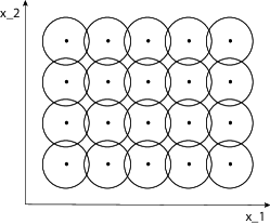
Figure 1: A receptive field is traditionally defined as a region in the visual field for which a visual sensor/neuron/operator responds to visual stimuli. This figure shows a set of partially overlapping receptive fields over the spatial domain with all the receptive fields having the same spatial extent. More generally, one can conceive distributions of receptive fields over space or space-time with the receptive fields of different size, different shape and orientation in space as well as different directions in space-time, where adjacent receptive fields may also have significantly larger relative overlap than shown in this schematic illustration. In this work, we focus on a functional description of linear receptive fields, concerning how a neuron responds to visual stimuli over image space regarding spatial receptive fields or over joint space-time regarding spatio-temporal receptive fields.

If one considers the theoretical and computational problem of designing a vision system that is going to make use of incoming reflected light to infer properties of the surrounding world, one may ask what types of image operations should be performed on the image data. Would any type of image operation be reasonable? Specifically regarding the notion of receptive fields one may ask what types of receptive field profiles would be reasonable. Is it possible to derive a theoretical model of how receptive fields “ought to” respond to visual data?

Initially, such a problem might be regarded as intractable unless the question can be further specified. It is, however, possible to address this problem systematically using approaches that have been developed in the area of computer vision known as scale-space theory (Iijima [6]; Witkin [7]; Koenderink [8]; Koenderink and van Doorn [9, 10]; Lindeberg [11, 12, 13, 14]; Florack [15]; Sporring et al. [16]; Weickert et al. [17]; ter Haar Romeny [18]). A paradigm that has been developed in this field is to impose structural constraints on the first stages of visual processing that reflect symmetry properties of the environment. Interestingly, it turns out to be possible to substantially reduce the class of permissible image operations from such arguments.

The subject of this article is to describe how structural requirements on the first stages of visual processing as formulated in scale-space theory can be used for deriving idealized functional models of visual receptive fields and implications of how these theoretical results can be used when modelling biological vision. A main theoretical argument is that idealized functional models for linear receptive fields can be derived by necessity given a small set of symmetry requirements that reflect properties of the world that one may naturally require an idealized vision system to be adapted to. In this respect, the treatment bears similarities to approaches in theoretical physics, where symmetry properties are often used as main arguments in the formulation of physical theories of the world. The treatment that will follow will be general in the sense that spatial, spatio-chromatic and spatio-temporal receptive fields are encompassed by the same unified theory.

This paper gives a condensed summary of a more general theoretical framework for receptive fields derived and presented in [13, 19, 20, 21] and in turn developed to enable a consistent handling of receptive field responses in terms of provable covariance or invariance properties under natural image transformations (see Figure 2). In relation to the early publications on this topic [13, 19, 20], this paper presents an improved version of that theory leading to an improved model for the temporal smoothing operation for the specific case of a time-causal image domain [21], where the future cannot be accessed and the receptive fields have to be solely based on information from the present moment and a compact buffer of the past. Specifically, this paper presents the improved axiomatic structure on a compact form more easy to access compared to the original publications and also encompassing the better time-causal model.

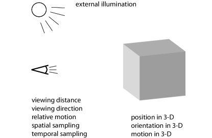
Figure 2: Basic factors that influence the formation of images for an eye with a two-dimensional retina that observes objects in the three-dimensional world. In addition to the position, the orientation and the motion of the object in 3-D, the perspective projection onto the retina is affected by the viewing distance, the viewing direction and the relative motion of the eye in relation to the object, the spatial and the temporal sampling characteristics of the neurons in the retina as well the usually unknown external illumination field in relation to the geometry of the scene and the observer.

It will be shown that the presented framework leads to predictions of receptive field profiles in good agreement with receptive measurements reported in the literature (Hubel and Wiesel [1, 2, 3]; DeAngelis et al. [4, 5]; Conway and Livingstone [22]; Johnson et al. [23]). Specifically, explicit phenomenological models will be given of LGN neurons and simple cells in V1 and will be compared to related models in terms of Gabor functions (Marčelja [24]; Jones and Palmer [25, 26]; Ringach [27, 28]), differences of Gaussians (Rodieck [29]) and Gaussian derivatives (Koenderink and van Doorn [9]; Young [30]; Young et al. [31, 32]). Notably, the evolution properties of the receptive field profiles in this model can be described by diffusion equations and are therefore suitable for implementation on a biological architecture, since the computations can be expressed in terms of communications between neighbouring computational units, where either a single computational unit or a group of computational units may be interpreted as corresponding to a neuron or a group of neurons. Specifically, computational models involving diffusion equations arise in mean field theory for approximating the computations that are performed by populations of neurons (Omurtag et al. [33]; Mattia and Guidic [34]; Faugeras et al. [35]).

1.1 Structure of this article

This paper is organized as follows: Section 2 gives an overview of and motivation to the assumptions that the theory is based on. A set of structural requirements is formulated to capture the effect of natural image transformations onto the illumination field that reaches the retina and to guarantee internal consistency between image representations that are computed from receptive field responses over multiple spatial and temporal scales.

Section 3 describes linear receptive families that arise as consequences of these assumptions for the cases of either a purely spatial domain or a joint spatio-temporal domain. The issue of how to perform relative normalization between receptive field responses over multiple spatial and temporal scales is treated, so as to enable comparisons between receptive field responses at different spatial and temporal scales. We also show how the influence of illumination transformations and exposure control mechanisms on the receptive field responses can be handled, by describing invariance properties obtained by applying the derived linear receptive fields over a logarithmically transformed intensity domain.

Section 4 shows examples of how spatial, spatio-chromatic and spatio-temporal receptive fields in the retina, the LGN and the primary visual cortex can be well modelled by the derived receptive field families.

Section 5 gives relations to previous work, including conceptual and theoretical comparisons to previous use of Gabor models of receptive fields, approaches for learning receptive fields from image data and previous applications of a logarithmic transformation of the image intensities. Finally, Section 6 summarizes some of the main results.

2 Assumptions underlying the theory: Structural requirements

In the following, we shall describe a set of structural requirements that can be stated concerning: (i) spatial geometry, (ii) spatio-temporal geometry, (iii) the image measurement process with its close relationship to the notion of scale, (iv) internal representations of image data that are to be computed by a general purpose vision system and (v) the parameterization of image intensity with regard to the influence of illumination variations.

For modelling the image formation process, we will at any point on the retina approximate the spherical retina by a perspective projection onto the tangent plane of the retinal surface at that image point, below represented as the image plane. Additionally, we will approximate the possibly non-linear geometric transformations regarding spatial and spatio-temporal geometry by local linearizations at every image point, and corresponding to the derivative of the possibly non-linear transformation. In these ways, the theoretical analysis can be substantially simplified, while still enabling accurate modelling of essential functional properties of receptive fields in relation to the effects of natural image transformations as arising from interactions with the environment.

2.1 Static image data over a spatial domain

In the following, we will describe a theoretical model for the computational function of applying visual receptive fields to local image patterns.

For time-independent data $f$ over a two-dimensional spatial image domain, we would like to define a family of image representations $L(\cdot;\;s)$ over a possibly multi-dimensional scale parameter $s$, where the internal image representations $L(\cdot;\;s)$ are computed by applying some parameterized family of image operators ${\cal T}_{s}$ to the image data $f$:

$$L(\cdot;\;s)={\cal T}_{s}\,f(\cdot).$$ (1)

Specifically, we will assume that the family of image operators ${\cal T}_{s}$ should satisfy:

Linearity

For the earliest processing stages to make as few irreversible decisions as possible, we assume that they should be linear

$${\cal T}_{s}(a_{1}f_{1}+a_{2}f_{2})=a_{1}{\cal T}_{s}f_{1}+b_{1}{\cal T}_{s}f_{2}.$$ (2)

Specifically, linearity implies that any particular scale-space properties (to be detailed below) that we derive for the zero-order image representation $L$ will transfer to any spatial derivative $L_{x_{1}^{\alpha_{1}}x_{2}^{\alpha_{2}}}$ of $L$, so that

$$L_{x_{1}^{\alpha_{1}}x_{2}^{\alpha_{2}}}(\cdot;\;s)=\partial_{x_{1}^{\alpha_{1}}x_{2}^{\alpha_{2}}}({\cal T}_{s}\,f)={\cal T}_{s}(\partial_{x_{1}^{\alpha_{1}}x_{2}^{\alpha_{2}}}f).$$ (3)

In this sense, the assumption of linearity reflects the requirement of a lack of bias to particular types of image structures, with the underlying aim that the processing performed in the first processing stages should be generic, to be used as input for a large variety of visual tasks. By the assumption of linearity, local image structures that are captured by e.g. first- or second-order derivatives will be treated in a structurally similar manner, which would not necessarily be the case if the first local neighbourhood processing stage of the first layer of receptive fields would instead be genuinely non-linear.

This genericity property is closely related to the basic property of the mammalian vision system, that the computations performed in the retina, the LGN and the primary visual cortex provide general purpose output that is used as input to higher-level visual areas.

Shift invariance

To ensure that the visual interpretation of an object should be the same irrespective of its position in the image plane, we assume that the first processing stages should be shift invariant, so that if an object is moved a distance $\Delta x=(\Delta x_{1},\Delta x_{2})$ in the image plane, the receptive field response should remain on a similar form while shifted with the same distance. Formally, this requirement can be stated that the family of image operators ${\cal T}_{s}$ should commute with the shift operator defined by $S_{\Delta x}(f)(x)=f(x-\Delta x)$:

$${\cal T}_{s}\left(S_{\Delta x}f\right)=S_{\Delta x}\left({\cal T}_{s}f\right).$$ (4)

In other words, if we shift the input by a translation and then apply the receptive field operator ${\cal T}_{s}$, the result should be similar as applying the receptive field operator to the original input and then shifting the result.

Convolution structure

Together, the assumptions about linearity and shift-invariance imply that ${\cal T}_{s}$ will correspond to a convolution operator [36]. This implies that the representation $L$ can be computed from the image data $f$ by convolution with some parameterized family of convolution kernels $T(\cdot;\;s)$:

$$L(\cdot;\;s)=T(\cdot;\;s)*f.$$ (5)

Semi-group structure over spatial scales

To ensure that the transformation from any finer scale $s_{1}$ to any coarser scale $s_{1}+s_{2}$ should be of the same form for any $s_{2}>0$ (a requirement of algebraic closedness), we assume that the result of convolving two kernels $T(\cdot;\;s_{1})$ and $T(\cdot;\;s_{2})$ from the family with each other should be a kernel within the same family of kernels and with added parameter values $T(\cdot;\;s_{1}+s_{2})$:

$$T(\cdot;\;s_{1})*T(\cdot;\;s_{2})=T(\cdot;\;s_{1}+s_{2}).$$ (6)

This assumption specifically implies that the representation $L(\cdot;\;s_{2})$ at a coarse scale $s_{2}$ can be computed from the representation $L(\cdot;\;s_{1})$ at a finer scale $s_{1}<s_{2}$ by a convolution operation of the same form (5) as the transformation from the original image data $f$ while using the difference in scale levels $s_{2}-s_{1}$ as the parameter

$$L(\cdot;\;s_{2})=T(\cdot;\;s_{2}-s_{1})*L(\cdot;\;s_{1}).$$ (7)

This property does in turn imply that if we are able to derive specific properties of the family of transformations ${\cal T}_{s}$ (to be detailed below), then these properties will not only hold for the transformation from the original image data $f$ to the representations $L(\cdot;\;s)$ at coarser scales, but also between any pair of scale levels $s_{2}>s_{1}$, with the aim that image representations at coarser scales should be possible to regard as simplifications of corresponding image representations at finer scales.

In terms of mathematical concepts, this form of algebraic structure is referred to as a semi-group structure over spatial scales

$${\cal T}_{s_{1}}{\cal T}_{s_{2}}={\cal T}_{s_{1}+s_{2}}.$$ (8)

Scale covariance under spatial scaling transformations

If a visual observer looks at the same object from different distances, we would like the internal representations derived from the receptive field responses to be sufficiently similar, so that the object can be recognized as the same object while appearing with a different size on the retina. Specifically, it is thereby natural to require that the receptive field responses should be of a similar form while resized in the image plane.

This corresponds to a requirement of spatial scale covariance under uniform scaling transformations of the spatial domain $x^{\prime}=S_{s}\,x$:

$$L^{\prime}(x^{\prime};\;s^{\prime})=L(x;\;s)\quad\Leftrightarrow\quad{\cal T}_{S_{s}(s)}\,{\cal S}_{s}\,f={\cal S}_{s}\,{\cal T}_{s}\,f$$ (9)

to hold for some transformation $s^{\prime}=S_{s}(s)$ of the scale parameter $s$.

Affine covariance under affine transformations

If a visual observer looks at the same local surface patch from two different viewing directions, then the local surface patch may be deformed in different ways onto the different views and with different amounts of perspective foreshortening from the different viewing directions. If we approximate the local deformations caused by the perspective mapping by local affine transformations, then the transformation between the two differently deformed views of the local surface patch can in turn be described by a composed local affine transformation $x^{\prime}=A\,x$. If we are to use receptive field responses as a basis for higher level visual operations, it is natural to require that the receptive field response of an affine deformed image patch should remain on a similar form while being reshaped by a corresponding affine transformation.

This corresponds to a requirement of affine covariance under general affine transformations $x^{\prime}=A\;x$:

$$L^{\prime}(x^{\prime};\;s^{\prime})=L(x;\;s)\quad\Leftrightarrow\quad{\cal T}_{A(s)}\,{\cal A}\,f={\cal A}\,{\cal T}_{s}\,f$$ (10)

to hold for some transformation $s^{\prime}=A(s)$ of the scale parameter.

Non-creation of new structure with increasing scale

If we apply the family of transformations ${\cal T}_{s}$ for computing representations at coarser scales from representations at finer scales according to (1) and (7), there could be a potential risk that the family of transformations could amplify spurious structures in the input to produce macroscopic amplifications in the representations at coarser scales that do not directly correspond to simplifications of corresponding structures in the original image data. To prevent such undesirable phenomena from occurring, we require that local spurious structures must not be amplified and express this condition in terms of the evolution properties over scales at local maxima and minima in the image intensities as smoothed by the family of convolution kernels $T(\cdot;\;s)$: If a point $x_{0}$ for some scale $s_{0}$ is a local maximum point in the image plane, then the value at this maximum point $L(x_{0};\;s_{0})$ must not increase to coarser scales $s>s_{0}$. Similarly, if a point is a local minimum point in the image plane, then the value at this minimum point $L(x_{0};\;s_{0})$ must not decrease to coarser scales $s>s_{0}$.

Formally, this requirement that new structures should not be created from finer to coarser scales, can be formalized into the requirement of non-enhancement of local extrema, which implies that if at some scale $s_{0}$ a point $x_{0}$ is a local maximum (minimum) for the mapping from $x$ to $L(x;\;s_{0})$, then (see Figure 3):

• $(\partial_{s}L)(x;\;s)\leq 0$ at any spatial maximum,

• $(\partial_{s}L)(x;\;s)\geq 0$ at any spatial minimum.

This condition implies a strong condition on the class of possible smoothing kernels $T(\cdot;\,s)$.

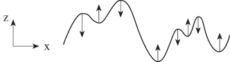
Figure 3: The requirement of non-enhancement of local extrema is a way of restricting the class of possible image operations by formalizing the notion that new image structures must not be created with increasing scale, by requiring that the value at a local maximum must not increase and that the value at a local minimum must not decrease from finer to coarser scales $s$.

2.2 Time-dependent image data over space-time

To model the computational function of spatio-temporal receptive fields in time-dependent image patterns, we do for a time-dependent spatio-temporal domain first inherit the structural requirements regarding a spatial domain and complement the spatial scale parameter $s$ by a temporal scale parameter $\tau$. In addition, we assume:

Scale covariance under temporal scaling transformations

If a similar type of spatio-temporal event $f(x,t)$ occurs at different speeds, faster or slower, it is natural to require that the receptive field responses should be of a similar form, while occurring correspondingly faster or slower.

This corresponds to a requirement of temporal scale covariance under a temporal scaling transformation of the temporal domain $t^{\prime}=S_{\tau}t$:

$$L^{\prime}(x^{\prime},t^{\prime};\;s^{\prime},\tau^{\prime})=L(x,t;\;s,\tau)\quad\Leftrightarrow\quad\\ {\cal T}_{S_{\tau}(s,\tau)}\,{\cal S}_{\tau}\,f={\cal S}_{\tau}\,{\cal T}_{s,\tau}\,f$$ (11)

to hold for some transformation $(s^{\prime},\tau^{\prime})=S_{\tau}(s,\tau)$ of the spatio-temporal scale parameters $(s,\tau)$.

Galilean covariance under Galilean transformations

If an observer looks at the same object in the world for different relative motions $v=(v_{1},v_{2})$ between the object and the observer, it is natural to require that the internal representations of the object should be sufficiently similar so as to enable a coherent perception of the object under different relative motions relative to the observer. Specifically, we may require that the receptive field responses under relative motions should remain on the same form while being transformed in a corresponding way as the relative motion pattern.

If we at any point in space-time locally linearize the possibly non-linear motion pattern $x(t)=(x_{1}(t),x_{2}(t))$ by a local Galilean transformation $x^{\prime}=x+v\,t$ over space-time

$$f^{\prime}={\cal G}_{v}\,f\quad\Leftrightarrow\quad f^{\prime}(x^{\prime},t^{\prime})=f(x,t)\quad\mbox{with}\quad x^{\prime}=x+v\,t,$$ (12)

then the requirement of guaranteeing a consistent visual interpretation under different relative motions between the object and the observer can be stated as a requirement of Galilean covariance:

$$L^{\prime}(x^{\prime},t^{\prime};\;s^{\prime},\tau^{\prime})=L(x,t;\;s,\tau)\quad\Leftrightarrow\quad\\ {\cal T}_{G_{v}(s,\tau)}\,{\cal G}_{v}\,f={\cal G}_{v}\,{\cal T}_{s,\tau}\,f$$ (13)

to hold for some transformation $G_{v}(s,\tau)$ of the spatio-temporal scale parameters $(s,\tau)$.

Semi-group structure over temporal scales in the case of a non-causal temporal domain

To ensure that the representations between different spatio-temporal scale levels $(s_{1},\tau_{1})$ and $(s_{2},\tau_{2})$ should be sufficiently well-behaved internally, we will make use of different types of assumptions depending on whether the temporal domain is regarded as time-causal or non-causal. Over a time-causal temporal domain, the future cannot be accessed, which is the basic condition for real-time visual perception by a biological organism. Over a non-causal temporal domain, the temporal kernels may extend to the relative future in relation to any pre-recorded time moment, which is sometimes used as a conceptual simplification when analysing pre-recorded time-dependent data although not at all realistic in a real-world setting.

For the case of a non-causal temporal domain, we make use of a similar type of semi-group property (8) as formulated over a purely spatial domain, while extending the semi-group property over both the spatial scale parameter $s$ and the temporal scale parameter $\tau$:

$${\cal T}_{s_{1},\tau_{1}}{\cal T}_{s_{2},\tau_{2}}={\cal T}_{s_{1}+s_{2},\tau_{1}+\tau_{2}}.$$ (14)

In analogy with the case of a purely spatial domain, this requirement guarantees that the transformation from any finer spatio-temporal scale level $(s_{1},\tau_{1})$ to any coarser spatio-temporal scale level $(s_{2},\tau_{2})\geq(s_{1},\tau_{1})$ will always be of the same form (algebraic closedness)

$$L(\cdot,\cdot;\;s_{2},\tau_{2})={\cal T}_{s_{2}-s_{1},\tau_{2}-\tau_{1}}\,L(\cdot,\cdot;\;s_{1},\tau_{1}).$$ (15)

Specifically, this assumption implies that if we are able to establish desirable properties of the family of transformations ${\cal T}_{s,\tau}$ (to be detailed below), then these relations hold between any pair of spatio-temporal scale levels $(s_{1},\tau_{1})$ and $(s_{2},\tau_{2})$ with $(s_{2},\tau_{2})\geq(s_{1},\tau_{1})$.

Cascade structure over temporal scales in the case of a time-causal temporal domain

Since it can be shown that the assumption of a semi-group structure over temporal scales leads to undesirable temporal dynamics in terms of e.g. longer temporal delays for a time-causal temporal domain [37, Appendix A], we do for a time-causal temporal domain instead assume a weaker cascade smoothing property over temporal scales for the temporal smoothing kernel over temporal scales

$$L(\cdot;\;\tau_{2})=h(\cdot;\;\tau_{1}\mapsto\tau_{2})*L(\cdot;\;\tau_{1}),$$ (16)

where the temporal kernels $h(t;\;\tau)$ should for any triplets of temporal scale values and temporal delays $\tau_{1}$, $\tau_{2}$ and $\tau_{3}$ obey the transitive property

$$h(\cdot;\;\tau_{1}\mapsto\tau_{2})*h(\cdot;\;\tau_{2}\mapsto\tau_{3})=h(\cdot;\;\tau_{1}\mapsto\tau_{3}).$$ (17)

This weaker assumption of a cascade smoothing property (16) still ensures that a representation at a coarser temporal scale $\tau_{2}$ should with a corresponding requirement of an accompanying simplifying condition on the family of kernels $h$ (to be detailed below) constitute a simplification of the representation at a finer temporal scale $\tau_{1}$, while not implying as hard constraints as a semi-group structure.

Non-enhancement of local space-time extrema in the case of a non-causal temporal domain

In the case of a non-causal temporal domain, we again build on the notion of non-enhancement of local extrema to guarantee that the representations at coarser spatio-temporal scales should constitute true simplifications of corresponding representations at finer scales Over a spatio-temporal domain, we do, however, state the requirement in terms of local extrema over joint space-time instead of over local extrema over image space. If a point $(x_{0},t_{0})$ for some scale $(s_{0},\tau_{0})$ is a local maximum point over space-time, then the value at this maximum point $L(x_{0},t_{0};\;s_{0},\tau_{0})$ must not increase to coarser scales $(s,\tau)\geq(s_{0},\tau_{0})$. Similarly, if a point is a local minimum point over space-time, then the value at this minimum point $L(x_{0},t_{0};\;s_{0},\tau_{0})$ must not decrease to coarser scales $(s,\tau)\geq(s_{0},\tau_{0})$.

Formally, this requirement of non-creation of new structure from finer to coarser spatio-temporal scales, can be stated as follows: If at some scale $(s_{0},\tau_{0})$ a point $(x_{0},t_{0})$ is a local maximum (minimum) for the mapping from $(x,t)$ to $L(x,t;\;s_{0},\tau_{0})$, then

• $\alpha\,(\partial_{s}L)(x,t;\;s,\tau)+\beta\,(\partial_{\tau}L)(x,t;\;s,\tau)\leq 0$ at any spatio-temporal maximum

• $\alpha\,(\partial_{s}L)(x,t;\;s,\tau)+\beta\,(\partial_{\tau}L)(x,t;\;s,\tau)\geq 0$ at any spatio-temporal minimum

should hold in any positive spatio-temporal direction defined from any non-negative linear combinations of $\alpha$ and $\beta$. This condition implies a strong condition on the class of possible smoothing kernels $T(\cdot,\cdot;\,s,\tau)$.

Non-creation of new local extrema or zero-crossings for a purely temporal signal in the case of a non-causal temporal domain

In the case of a time-causal temporal domain, we do instead state a requirement for purely temporal signals, based on the cascade smoothing property (16). We require that for a purely temporal signal $f(t)$, the transformation from a finer temporal scale $\tau_{1}$ to a coarser temporal scale $\tau_{2}$ must not increase the number of local extrema or the number of zero-crossings in the signal.

$g(x_{1},x_{2};\;s)$

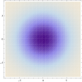
$g_{x_{1}}(x_{1},x_{2};\;s)$	$g_{x_{2}}(x_{1},x_{2};\;s)$

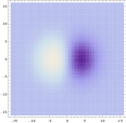
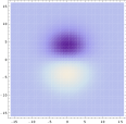
$g_{x_{1}x_{1}}(x_{1},x_{2};\;s)$	$g_{x_{1}x_{2}}(x_{1},x_{2};\;s)$	$g_{x_{2}x_{2}}(x_{1},x_{2};\;s)$

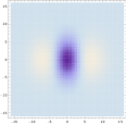
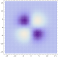
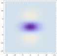
Figure 4: Spatial receptive fields formed by the 2-D Gaussian kernel with its partial derivatives up to order two. The corresponding family of receptive fields is closed under translations, rotations and scaling transformations, meaning that if the underlying image is subject to a set of such image transformations then it will always be possible to find some possibly other receptive field such that the receptive field responses of the original image and the transformed image can be matched.

$g(x;\;\Sigma_{1})$	$g(x;\;\Sigma_{2})$	$g(x;\;\Sigma_{3})$

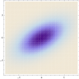
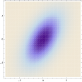
$g_{\varphi_{1}}(x;\;\Sigma_{1})$	$g_{\varphi_{2}}(x;\;\Sigma_{2})$	$g_{\varphi_{3}}(x;\;\Sigma_{3})$

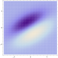
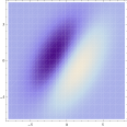
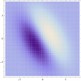
$g_{\varphi_{1}\varphi_{1}}(x;\;\Sigma_{1})$	$g_{\varphi_{2}\varphi_{2}}(x;\;\Sigma_{2})$	$g_{\varphi_{3}\varphi_{3}}(x;\;\Sigma_{3})$

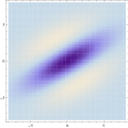
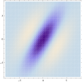
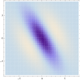
Figure 5: Spatial receptive fields formed by affine Gaussian kernels and directional derivatives of these, here using three different covariance matrices $\Sigma_{1}$, $\Sigma_{2}$ and $\Sigma_{3}$ corresponding to the directions $\theta_{1}=\pi/6$, $\theta_{2}=\pi/3$ and $\theta_{3}=2\pi/3$ of the major eigendirection of the covariance matrix and with first- and second-order directional derivatives computed in the corresponding orthogonal directions $\varphi_{1}$, $\varphi_{2}$ and $\varphi_{3}$. The corresponding family of receptive fields is closed under general affine transformations of the spatial domain, including translations, rotations, scaling transformations and perspective foreshortening (although this figure only illustrates variabilities in the orientation of the filter, thereby disregarding variations in both the size and the degree of elongation). This closedness property implies that receptive field responses computed from different views of a smooth local surface patch can be perfectly matched, if the transformation between the two views can be modelled as a local affine transformation.

3 Idealized receptive field families

3.1 Spatial image domain

Based on the above assumptions in Section 2.1, it can be shown [13] that when complemented with certain regularity assumptions in terms of Sobolev norms, they imply that a spatial scale-space representation $L$ as determined by these must satisfy a diffusion equation of the form

$$\partial_{s}L=\frac{1}{2}\nabla^{T}\left(\Sigma_{0}\nabla L\right)-\delta_{0}^{T}\nabla L$$ (18)

for some positive semi-definite covariance matrix $\Sigma_{0}$ and some translation vector $\delta_{0}$. In terms of convolution kernels, this corresponds to Gaussian kernels of the form

$$g(x;\;\Sigma_{s},\delta_{s})=\frac{1}{(2\pi)^{N/2}\sqrt{\det\Sigma_{s}}}\,e^{-{(x-\delta_{s})^{T}\Sigma_{s}^{-1}(x-\delta_{s})}/{2}},$$ (19)

which for a given $\Sigma_{s}=s\,\Sigma_{0}$ and a given $\delta_{s}=s\,\delta_{0}$ satisfy (18). If we additionally require these kernels to be mirror symmetric through the origin, then we obtain affine Gaussian kernels

$$g(x;\;\Sigma)=\frac{1}{(2\pi)^{N/2}\sqrt{\det\Sigma}}\,e^{-x^{T}\Sigma^{-1}x/2}.$$ (20)

Their spatial derivatives constitute a canonical family for expressing receptive fields over a spatial domain that can be summarized on the form

$$T(x;\;s,\Sigma)=g(x;\;s\,\Sigma).$$ (21)

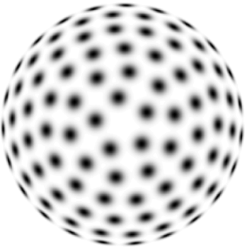
Figure 6: Distribution of affine Gaussian receptive fields corresponding to a uniform distribution on a hemisphere regarding zero-order smoothing kernels. In the most idealized version of the theory, one can think of all affine receptive fields with their directional derivatives in preferred directions aligned to the eigendirections of the covariance matrix $\Sigma$ as being present at any position in the image domain. When restricted to a limited number of receptive fields in an actual implementation, there is also an issue of distributing a fixed number of receptive fields over the spatial coordinates $x=(x_{1},x_{2})$ and the filter parameters $s$ and $\Sigma$.

Incorporating the fact that spatial derivatives of these kernels are also compatible with the assumptions underlying this theory, this does specifically for the case of a two-dimensional spatial image domain lead to spatial receptive fields that can be compactly summarized on the form

$$T_{{\varphi}^{m_{1}}{\bot{\varphi}}^{m_{2}}}(x_{1},x_{2};\;s,\Sigma)=\partial_{\varphi}^{m_{1}}\partial_{\bot\varphi}^{m_{2}}\left(g(x_{1},x_{2};\;s\Sigma)\right),$$ (22)

where

• $x=(x_{1},x_{2})$ denote the spatial coordinates,

• $s$ denotes the spatial scale,

• $\Sigma$ denotes a spatial covariance matrix determining the shape of a spatial affine Gaussian kernel,

• $m_{1}$ and $m_{2}$ denote orders of spatial differentiation,

• $\partial_{\varphi}=\cos\varphi\,\partial_{x_{1}}+\sin\varphi\,\partial_{x_{2}}$, $\partial_{\bot\varphi}=\sin\varphi\,\partial_{x_{1}}-\cos\varphi\,\partial_{x_{2}}$ denote spatial directional derivative operators in two orthogonal directions $\varphi$ and $\bot\varphi$ aligned with the eigenvectors of the covariance matrix $\Sigma$,

• $g(x;\;s,\Sigma)=\frac{1}{2\pi s\sqrt{\det\Sigma}}e^{-x^{T}\Sigma^{-1}x/2s}$ is an affine Gaussian kernel with its size determined by the spatial scale parameter $s$ and its shape by the spatial covariance matrix $\Sigma$.

Figure 5 and Figure 5 show examples of spatial receptive fields from this family up to second order of spatial differentiation. Figure 5 shows partial derivatives of the Gaussian kernel for the specific case when the covariance matrix $\Sigma$ is restricted to a unit matrix and the Gaussian kernel thereby becomes rotationally symmetric. The resulting family of receptive fields is closed under scaling transformations over the spatial domain, implying that if an object is seen from different distances to the observer, then it will always be possible to find a transformation of the scale parameter $s$ between the two image domains so that the receptive field responses computed from the two image domains can be matched. Figure 5 shows examples of affine Gaussian receptive fields for covariance matrices $\Sigma$ that do not correspond to rescaled copies of the unit matrix. The resulting full family of affine Gaussian derivative kernels is closed under general affine transformations, implying that for two different perspective views of a local smooth surface patch, it will always be possible to find a transformation of the covariance matrices $\Sigma$ between the two domains so that the receptive field responses can be matched, if the transformation between the two image domains is approximated by a local affine transformation.

In the most idealized version of the theory, one should think of receptive fields for all combinations of filter parameters as being present at every image point, as illustrated in Figure 6 concerning affine Gaussian receptive fields over different orientations in image space and different eccentricities.

3.2 Spatio-temporal image domain

Over a non-causal spatio-temporal domain, corresponding arguments as in Section 3.1 lead to a similar form of diffusion equation as in Equation (18), while expressed over the joint space-time domain $p=(x,t)$ and with $\delta_{0}$ interpreted as a local drift velocity. After splitting the composed affine Gaussian spatio-temporal smoothing kernel corresponding to (19) while expressed over the joint space-time domain into separate smoothing operations over space and time, this leads to zero-order spatio-temporal receptive fields of the form [13, 19]:

$$T(x_{1},x_{2},t;\;s,\tau;\;v,\Sigma)=g(x_{1}-v_{1}t,x_{2}-v_{2}t;\;s,\Sigma)\,h(t;\;\tau).$$ (23)

After combining that result with the results from corresponding theoretical analysis for a time-causal spatio-temporal domain in [13, 21], the resulting spatio-temporal derivative kernels constituting the spatio-temporal extension of the spatial receptive field model (22) can be reparametrised and summarized on the following form (see [13, 19, 20, 21]):

$$\begin{split}&T_{{\varphi}^{m_{1}}{\bot\varphi}^{m_{2}}{\bar{t}}^{n}}(x_{1},x_{2},t;\;s,\tau;\;v,\Sigma)\end{split}$$

$$\begin{split}&=\partial_{\varphi}^{m_{1}}\partial_{\bot\varphi}^{m_{2}}\partial_{\bar{t}}^{n}\left(g(x_{1}-v_{1}t,x_{2}-v_{2}t;\;s,\Sigma)\,h(t;\;\tau)\right),\end{split}$$ (24)

where

• $x=(x_{1},x_{2})$ denote the spatial coordinates,

• $t$ denotes time,

• $s$ denotes the spatial scale,

• $\tau$ denotes the temporal scale,

• $v=(v_{1},v_{2})^{T}$ denotes a local image velocity,

• $\Sigma$ denotes a spatial covariance matrix determining the shape of a spatial affine Gaussian kernel,

• $m_{1}$ and $m_{2}$ denote orders of spatial differentiation,

• $n$ denotes the order of temporal differentiation,

• $\partial_{\varphi}=\cos\varphi\,\partial_{x_{1}}+\sin\varphi\,\partial_{x_{2}}$ and $\partial_{\bot\varphi}=\sin\varphi\,\partial_{x_{1}}-\cos\varphi\,\partial_{x_{2}}$ denote spatial directional derivative operators in two orthogonal directions $\varphi$ and $\bot\varphi$ aligned with the eigenvectors of the covariance matrix $\Sigma$,

• $\partial_{\bar{t}}=v_{1}\partial_{x_{1}}+v_{2}\partial_{x_{2}}+\partial t$ is a velocity-adapted temporal derivative operator aligned to the direction of the local image velocity $v=(v_{1},v_{2})^{T}$,

• $g(x;\;s,\Sigma)=\frac{1}{2\pi s\sqrt{\det\Sigma}}e^{-x^{T}\Sigma^{-1}x/2s}$ is an affine Gaussian kernel with its size determined by the spatial scale parameter $s$ and its shape determined by the spatial covariance matrix $\Sigma$,

• $g(x_{1}-v_{1}t,x_{2}-v_{2}t;\;s,\Sigma)$ denotes a spatial affine Gaussian kernel that moves with image velocity $v=(v_{1},v_{2})$ in space-time and

• $h(t;\;\tau)$ is a temporal smoothing kernel over time corresponding to a Gaussian kernel $h(t;\;\tau)=g(t;\;\tau)=1/\sqrt{2\pi\tau}\exp(-t^{2}/2\tau)$ in the case of non-causal time or a cascade of first-order integrators or equivalently truncated exponential kernels coupled in cascade $h(t;\;\tau)=h_{composed}(\cdot;\;\mu)$ according to (26) over a time-causal temporal domain.

This family of spatio-temporal scale-space kernels can be seen as a canonical family of linear receptive fields over a spatio-temporal domain.

For the case of a time-causal temporal domain, the result states that truncated exponential kernels of the form

$$h_{exp}(t;\;\mu_{k})=\left\{\begin{array}[]{ll}\frac{1}{\mu_{k}}e^{-t/\mu_{k}}&t\geq 0\\ 0&t<0\end{array}\right.$$ (25)

coupled in cascade constitute the natural temporal smoothing kernels. These do in turn lead to a composed temporal convolution kernel of the form

$$h_{composed}(\cdot;\;\mu)=*_{k=1}^{K}h_{exp}(\cdot;\;\mu_{k})$$ (26)

and corresponding to a set of first-order integrators coupled in cascade (see Figure 7).

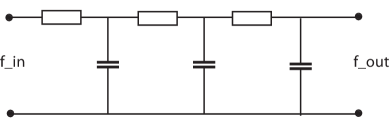
Figure 7: Electric wiring diagram consisting of a set of resistors and capacitors that emulate a series of first-order integrators coupled in cascade, if we regard the time-varying voltage $f_{in}$ as representing the time varying input signal and the resulting output voltage $f_{out}$ as representing the time varying output signal at a coarser temporal scale. According to the theory of temporal scale-space kernels for one-dimensional signals (Lindeberg [38, 21]; Lindeberg and Fagerström [39]), the corresponding equivalent truncated exponential kernels are the only primitive temporal smoothing kernels that guarantee both temporal causality and non-creation of local extrema (alternatively zero-crossings) with increasing temporal scale.

$-T(x,t;\;s,\tau)$

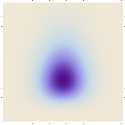
$T_{x}(x,t;\;s,\tau)$	$T_{t}(x,t;\;s,\tau,\delta)$

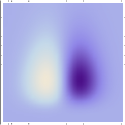
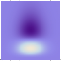
$T_{xx}(x,t;\;s,\tau)$	$T_{xt}(x,t;\;s,\tau)$	$T_{tt}(x,t;\;s,\tau)$

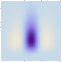
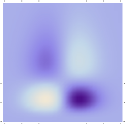
Figure 8: Space-time separable kernels $T_{x^{m}t^{n}}(x,t;\;s,\tau)=\partial_{x^{m}t^{n}}(g(x;\;s)\,h(t;\;\tau))$ up to order two obtained as the composition of Gaussian kernels over the spatial domain $x$ and a cascade of truncated exponential kernels over the temporal domain $t$ with a logarithmic distribution of the intermediate temporal scale levels that approximates the time-causal limit kernel ($s=1$, $\tau=1$, $K=7$, $c=\sqrt{2}$). The corresponding family of spatio-temporal receptive fields is closed under spatial scaling transformations as well as under temporal scaling transformations for temporal scaling factors that are integer powers of the distribution parameter $c$ of the temporal smoothing kernel. (Horizontal axis: space $x$. Vertical axis: time $t$.)

$-T(x,t;\;s,\tau,v)$

$T_{x}(x,t;\;s,\tau,v)$	$T_{t}(x,t;\;s,\tau,\delta)$

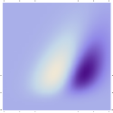
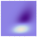
$T_{xx}(x,t;\;s,\tau,v)$	$T_{xt}(x,t;\;s,\tau,v)$	$T_{tt}(x,t;\;s,\tau,v)$

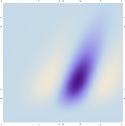
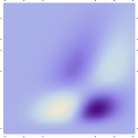
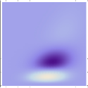
Figure 9: Velocity-adapted spatio-temporal kernels $T_{x^{m}t^{n}}(x,t;\;s,\tau,v)=\partial_{x^{m}t^{n}}(g(x-vt;\;s)\,h(t;\;\tau))$ up to order two obtained as the composition of Gaussian kernels over the spatial domain $x$ and a cascade of truncated exponential kernels over the temporal domain $t$ with a logarithmic distribution of the intermediate temporal scale levels that approximates the time-causal limit kernel ($s=1$, $\tau=1$, $K=7$, $c=\sqrt{2}$, $v=0.5$). In addition to spatial and temporal scaling transformations, the corresponding family of receptive fields is also closed under Galilean transformations. (Horizontal axis: space $x$. Vertical axis: time $t$.)

Two natural ways of distributing the discrete time constants $\mu_{k}$ over temporal scales are studied in detail in [21, 37] corresponding to either a uniform or a logarithmic distribution in terms of the composed variance

$$\tau_{K}=\sum_{k=1}^{K}\mu_{k}^{2}.$$ (27)

Specifically, it is shown in [21] that in the case of a logarithmic distribution of the discrete temporal scale levels, it is possible to consider an infinite number of temporal scale levels that cluster infinitely dense near zero temporal scale

$$\dots\frac{\tau_{0}}{c^{6}},\frac{\tau_{0}}{c^{4}},\frac{\tau_{0}}{c^{2}},\tau_{0},c^{2}\tau_{0},c^{4}\tau_{0},c^{6}\tau_{0},\dots$$ (28)

so that a scale-invariant time-causal limit kernel $\Psi(t;\;\tau,c)$ can be defined obeying self-similarity and scale covariance over temporal scales and with a Fourier transform of the form

$$\hat{\Psi}(\omega;\;\tau,c)=\prod_{k=1}^{\infty}\frac{1}{1+i\,c^{-k}\sqrt{c^{2}-1}\sqrt{\tau}\,\omega}.$$ (29)

Figure 9 and Figure 9 show spatio-temporal kernels over a 1+1-dimensional spatio-temporal domain using approximations of the time-causal limit kernel for temporal smoothing over the temporal domain and the Gaussian kernel for spatial smoothing over the spatial domain. Figure 9 shows space-time separable receptive fields corresponding to image velocity $v=0$, whereas Figure 9 shows unseparable velocity-adapted receptive fields corresponding to a non-zero image velocity $v\neq 0$.

The family of space-time separable receptive fields for zero image velocities is closed under spatial scaling transformations for arbitrary spatial scaling factors as well as for temporal scaling transformations with temporal scaling factors that are integer powers of the distribution parameter $c$ of the time-causal limit kernel. The full family of velocity-adapted receptive fields for general non-zero image velocities is additionally closed under Galilean transformations, corresponding to variations in the relative motion between the objects in the world and the observer. Given that the full families of receptive fields are explicitly represented in the vision system, this means that it will be possible to perfectly match receptive field responses computed under the following types of natural image transformations: (i) objects of different size in the image domain as arising from e.g. viewing the same object from different distances, (ii) spatio-temporal events that occur with different speed, faster or slower, and (iii) objects and spatio-temporal that are viewed with different relative motions between the objects/event and the visual observer.

If additionally the spatial smoothing is performed over the full family of spatial covariance matrices $\Sigma$, then receptive field responses can also be matched (iv) between different views of the same smooth local surface patch.

3.3 Scale normalisation of spatial and spatio-temporal receptive fields

When computing receptive field responses over multiple spatial and temporal scales, there is an issue about how the receptive field responses should be normalized so as to enable appropriate comparisons between receptive field responses at different scales. Issues of scale normalisation of the derivative based receptive fields defined from scale-space operations are treated in [40, 41, 42] regarding spatial receptive fields and in [21, 37, 43] regarding spatio-temporal receptive fields.

Scale-normalized spatial receptive fields

Let $s_{\varphi}$ and $s_{\bot{\varphi}}$ denote the eigenvalues of the composed affine covariance matrix $s\,\Sigma$ in the spatial receptive field model (22) and let $\partial_{\varphi}$ and $\partial_{\bot{\varphi}}$ denote directional derivative operators along the corresponding eigendirections. Then, the scale-normalized spatial derivative kernel corresponding to the receptive field model (22) is given by

$$T_{{\varphi}^{m_{1}}{\bot{\varphi}}^{m_{2}},norm}(x_{1},x_{2};\;s,\Sigma)=\\ s_{\varphi}^{m_{1}\gamma_{s}/2}\,s_{\bot{\varphi}}^{m_{2}\gamma_{s}/2}\,\partial_{\varphi}^{m_{1}}\partial_{\bot\varphi}^{m_{2}}\left(g(x_{1},x_{2};\;s\Sigma)\right),$$ (30)

where $\gamma_{s}$ denotes the spatial scale normalization parameter of $\gamma$-normalized derivatives and specifically the choice $\gamma_{s}=1$ leads to maximum scale invariance in the sense that the magnitude response of the spatial receptive field will be covariant under uniform spatial scaling transformations $(x_{1}^{\prime},x_{2}^{\prime})=(S_{s}\,x_{1},S_{s}\,x_{2})$, provided that the spatial scale levels are appropriately matched $(s_{\varphi}^{\prime},s_{\bot{\varphi}}^{\prime})=(S_{s}^{2}\,s_{\varphi},S_{s}^{2}\,s_{\bot{\varphi}})$.

Scale-normalized spatial receptive fields in the case of a non-causal spatio-temporal domain

For the case of a non-causal spatio-temporal domain, where the temporal smoothing operation in the spatio-temporal receptive field model is performed by a non-causal Gaussian temporal kernel $h(t;\;\tau)=g(t;\;\tau)=1/\sqrt{2\pi\tau}\exp(-t^{2}/2\tau)$, the scale-normalized spatio-temporal derivative kernel corresponding to the spatio-temporal receptive field model (LABEL:eq-spat-temp-RF-model-der) is with corresponding notation regarding the spatial domain as in (30) given by

$$\begin{split}&T_{{\varphi}^{m_{1}}{\bot\varphi}^{m_{2}}{\bar{t}}^{n},norm}(x_{1},x_{2},t;\;s,\tau;\;v,\Sigma)\end{split}$$

$$\begin{split}&=s_{\varphi}^{m_{1}\gamma_{s}/2}\,s_{\bot{\varphi}}^{m_{2}\gamma_{s}/2}\,\tau^{n\gamma_{\tau}/2}\,\end{split}$$

$$\begin{split}&\phantom{=}\,\,\,\,\partial_{\varphi}^{m_{1}}\partial_{\bot\varphi}^{m_{2}}\partial_{\bar{t}}^{n}\left(g(x_{1}-v_{1}t,x_{2}-v_{2}t;\;s,\Sigma)\,h(t;\;\tau)\right),\end{split}$$ (31)

where $\gamma_{s}$ and $\gamma_{\tau}$ denote the spatial and temporal scale normalization parameters of $\gamma$-normalized derivatives and specifically the choice $\gamma_{s}=1$ and $\gamma_{\tau}=1$ leads to maximum scale invariance in the sense that the magnitude response of the spatio-temporal receptive field will be invariant under independent scaling transformations of the spatial and the temporal domains $(x_{1}^{\prime},x_{2}^{\prime},t^{\prime})=(S_{s}\,x_{1},S_{s}\,x_{2},S_{\tau}\,t)$, provided that both the spatial and temporal scale levels are appropriately matched $(s_{\varphi}^{\prime},s_{\bot{\varphi}}^{\prime},\tau^{\prime})=(S_{s}^{2}\,s_{\varphi},S_{s}^{2}\,s_{\bot{\varphi}},S_{\tau}^{2}\,\tau)$.

Scale-normalized spatial receptive fields in the case of a time-causal spatio-temporal domain

For the case of a time-causal spatio-temporal domain, where the temporal smoothing operation in the spatio-temporal receptive field model is performed by truncated exponential kernels coupled in cascade $h(t;\;\tau)=h_{composed}(\cdot;\;\mu)$ (26), the corresponding scale-normalized spatio-temporal derivative kernel corresponding to the spatio-temporal receptive field model (LABEL:eq-spat-temp-RF-model-der) is given by

$$\begin{split}&T_{{\varphi}^{m_{1}}{\bot\varphi}^{m_{2}}{\bar{t}}^{n},norm}(x_{1},x_{2},t;\;s,\tau;\;v,\Sigma)\end{split}$$

$$\begin{split}&=s_{\varphi}^{m_{1}\gamma_{s}/2}\,s_{\bot{\varphi}}^{m_{2}\gamma_{s}/2}\,\alpha_{n,\gamma_{\tau}}(\tau)\,\end{split}$$

$$\begin{split}&\phantom{=}\,\,\,\,\partial_{\varphi}^{m_{1}}\partial_{\bot\varphi}^{m_{2}}\partial_{\bar{t}}^{n}\left(g(x_{1}-v_{1}t,x_{2}-v_{2}t;\;s,\Sigma)\,h(t;\;\tau)\right),\end{split}$$ (32)

where $\gamma_{s}$ and $\gamma_{\tau}$ denote the spatial and and temporal scale normalization parameters of $\gamma$-normalized derivatives and $\alpha_{n,\gamma_{\tau}}(\tau)$ is the temporal scale normalization factor, which for the case of variance-based normalization is given by

$$\alpha_{n,\gamma_{\tau}}(\tau)=\tau^{n\gamma_{\tau}/2}$$ (33)

in agreement with (LABEL:eq-spat-temp-RF-model-der-norm-non-caus) while for the case of $L_{p}$-normalization it is given by [21, Equation (76)]

$$\alpha_{n,\gamma_{\tau}}(\tau)=\frac{G_{n,\gamma_{\tau}}}{\|h_{t^{n}}(\cdot;\;\tau)\|_{p}},$$ (34)

with $G_{n,\gamma_{\tau}}$ denoting the $L_{p}$-norm of the $n$th order scale-normalized derivative of a non-causal Gaussian temporal kernel with scale normalization parameter $\gamma_{\tau}$. In the specific case when the temporal smoothing is performed using the scale-invariant limit kernel (29), the magnitude response will for the maximally scale invariant choice of scale normalization parameters $\gamma_{s}=1$ and $\gamma_{\tau}=1$ be invariant under independent scaling transformations of the spatial and the temporal domains $(x_{1}^{\prime},x_{2}^{\prime},t^{\prime})=(S_{s}\,x_{1},S_{s}\,x_{2},S_{\tau}\,t)$ for general spatial scaling factors $S_{s}$ and for temporal scaling factors $S_{\tau}=c^{j}$ that are integer powers of the distribution parameter $c$ of the scale-invariant limit kernel, provided that both the spatial and temporal scale levels are appropriately matched $(s_{\varphi}^{\prime},s_{\bot{\varphi}}^{\prime},\tau^{\prime})=(S_{s}^{2}\,s_{\varphi},S_{s}^{2}\,s_{\bot{\varphi}},S_{\tau}^{2}\,\tau)$.

3.4 Invariance to local multiplicative illumination variations or variations in exposure parameters

The treatment so far has been concerned with modelling receptive fields under natural geometric image transformations, modelled as local scaling transformations, local affine transformations and local Galilean transformations representing the essential dimensions in the variability of a local linearization of the perspective mapping from a local surface patch in the world to the tangent plane of the retina. A complementary issue concerns how to model receptive field responses under variations in the external illumination and under variations in the internal exposure mechanisms of the eye that adapt the diameter of the pupil and the sensitivity of the photoreceptors to the external illumination. In this section, we will present a solution for this problem regarding the subset of intensity transformations that can be modelled as local multiplicative intensity transformations.

To obtain theoretically well-founded handling of image data under illumination variations, it is natural to represent the image data on a logarithmic luminosity scale

$$f(x_{1},x_{2},t)\sim\log I(x_{1},x_{2},t).$$ (35)

Specifically, receptive field responses that are computed from such a logarithmic parameterization of the image luminosities can be interpreted physically as a superposition of relative variations of surface structure and illumination variations. Let us assume: (i) a perspective camera model extended with (ii) a thin circular lens for gathering incoming light from different directions and (iii) a Lambertian illumination model extended with (iv) a spatially varying albedo factor for modelling the light that is reflected from surface patterns in the world. Then, it can be shown [19, Section 2.3] that a spatio-temporal receptive field response

$$L_{{\varphi}^{m_{1}}{\bot\varphi}^{m_{2}}{\bar{t}}^{n}}(\cdot,\cdot;\;s, \tau)=\partial_{{\varphi}^{m_{1}}{\bot\varphi}^{m_{2}}{\bar{t}}^{n}}\,{\cal T}_{s,\tau}\,f(\cdot,\cdot)$$ (36)

of the image data $f$, where ${\cal T}_{s,\tau}$ represents the spatio-temporal smoothing operator (here corresponding to a spatio-temporal smoothing kernel of the form (23)) can be expressed as

$$\begin{split}&L_{{\varphi}^{m_{1}}{\bot\varphi}^{m_{2}}{\bar{t}}^{n}}(x_{1},x_{2},t;\;s,\tau)=\\ \end{split}$$

$$\begin{split}&=\partial_{{\varphi}^{m_{1}}{\bot\varphi}^{m_{2}}{\bar{t}}^{n}}\,{\cal T}_{s,\tau}\,\left(\log\rho(x_{1},x_{2},t)+\log i(x_{1},x_{2},t)\vphantom{\log C_{cam}(\tilde{f}(t))}\right.\end{split}$$

$$\begin{split}&\phantom{=\partial_{{\varphi}^{m_{1}}{\bot\varphi}^{m_{2}}{\bar{t}}^{n}}\,{\cal T}_{s,\tau}\,\left(\right.}\left.+\log C_{cam}(\tilde{f}(t))+V(x_{1},x_{2})\right),\end{split}$$ (37)

where

• $\rho(x_{1},x_{2},t)$ is a spatially dependent albedo factor that reflects properties of surfaces of objects in the environment with the implicit understanding that this entity may in general refer to points on different surfaces in the world depending on the viewing direction and thus the (possibly time-dependent) image position $(x(t),y(t))$,

• $i(x_{1},x_{2},t)$ denotes a spatially dependent illumination field with the implicit understanding that the amount of incoming light on different surfaces may be different for different points in the world as mapped to corresponding image coordinates $(x_{1},x_{2})$ over time $t$,

• $C_{cam}(\tilde{f}(t))=\frac{\pi}{4}\frac{d}{f}$ represents the possibly time-dependent internal camera parameters with the ratio $\tilde{f}=f/d$ referred to as the effective $f$-number, where $d$ denotes the diameter of the lens and $f$ the focal distance, and

• $V(x_{1},x_{2})=-2\log(1+x_{1}^{2}+x_{2}^{2})$ represents a geometric natural vignetting effect corresponding to the factor $\log\cos^{4}(\phi)$ for a planar image plane, with $\phi$ denoting the angle between the viewing direction $(x_{1},x_{2},f)$ and the surface normal $(0,0,1)$ of the image plane. This vignetting term disappears for a spherical camera model.

From the structure of Equation (LABEL:eq-illum-model-spat-rec-field) we can note that for any non-zero order of spatial differentiation with at least either $m_{1}>0$ or $m_{2}>0$, the influence of the internal camera parameters in $C_{cam}(\tilde{f}(t))$ will disappear because of the spatial differentiation with respect to $x_{1}$ or $x_{2}$, and so will the effects of any other multiplicative exposure control mechanism. Furthermore, for any multiplicative illumination variation $i^{\prime}(x_{1},x_{2})=C\,i(x_{1},x_{2})$, where $C$ is a scalar constant, the logarithmic luminosity will be transformed as $\log i^{\prime}(x_{1},x_{2})=\log C+\log i(x_{1},x_{2})$, which implies that the dependency on $C$ will disappear after spatial or temporal differentiation.

Thus, given that the image measurements are performed on a logarithmic brightness scale, the spatio-temporal receptive field responses will be automatically invariant under local multiplicative illumination variations as well as under local multiplicative variations in the exposure parameters of the retina and the eye.

4 Computational modelling of biological receptive fields

In two comprehensive reviews, DeAngelis et al. [4, 5] present overviews of spatial and temporal response properties of (classical) receptive fields in the central visual pathways. Specifically, the authors point out the limitations of defining receptive fields in the spatial domain only and emphasize the need to characterize receptive fields in the joint space-time domain, to describe how a neuron processes the visual image. Conway and Livingstone [22] and Johnson et al. [23] show results of corresponding investigations concerning spatio-chromatic receptive fields.

In the following, we will describe how the above derived idealized functional models of linear receptive fields can be used for modelling the spatial, spatio-chromatic and spatio-temporal response properties of biological receptive fields. Indeed, it will be shown that the derived idealized functional models lead to predictions of receptive field profiles that are qualitatively very similar to all the receptive field types presented in (DeAngelis et al. [4, 5]) and schematic simplifications of most of the receptive fields shown in (Conway and Livingstone [22]) and (Johnson et al. [23]).

$h_{xxt}(x,t;\;s,\tau)$	$-h_{xxtt}(x,t;\;s,\tau)$

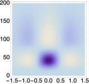
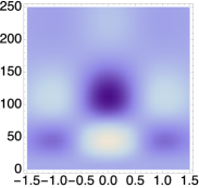
Figure 10: Computational modelling of space-time separable receptive field profiles in the lateral geniculate nucleus (LGN) as reported by DeAngelis et al. [4] using idealized spatio-temporal receptive fields of the form $T(x,t;\;s,\tau)=\partial_{x^{m}}\partial_{t^{n}}(g(;\;s)\,h(t;\;\tau))$ according to Equation (LABEL:eq-spat-temp-RF-model-der) with the temporal smoothing function $h(t;\;\tau)$ modelled as a cascade of first-order integrators/truncated exponential kernels of the form (26): (left) a “non-lagged cell” modelled using first-order temporal derivatives, (right) a “lagged cell” modelled using second-order temporal derivatives. Parameter values with $\sigma_{x}=\sqrt{s}$ and $\sigma_{t}=\sqrt{\tau}$: (a) $h_{xxt}$: $\sigma_{x}=0.5$ degrees, $\sigma_{t}=40$ ms. (b) $h_{xxtt}$: $\sigma_{x}=0.6$ degrees, $\sigma_{t}=60$ ms. (Horizontal dimension: space $x$. Vertical dimension: time $t$.)

	$\nabla^{2}g(x,y;\;s)$

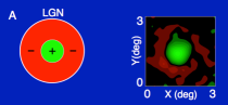
Figure 11: Computational modelling the spatial component of receptive fields in the LGN using the Laplacian of the Gaussian: (left) Receptive fields in the LGN have approximately circular center-surround responses in the spatial domain, as reported by DeAngelis et al. [4]. (right) In terms of Gaussian derivatives, this spatial response profile can be modelled by the Laplacian of the Gaussian $\nabla^{2}g(x,y;\;s)=(x^{2}+y^{2}-2s)/(2\pi s^{3})\exp(-(x^{2}+y^{2})/2s)$, here with $\sigma_{s}=\sqrt{s}=0.6$ in units of degrees of visual angle.

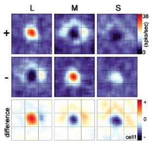
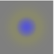
Figure 12: Spatio-chromatic receptive field response of a double-opponent neuron as reported by Conway and Livingstone [22, Figure 2, Page 10831], with the colour channels L, M and S essentially corresponding to red, green and blue, respectively. (From these L, M and S colour channels, corresponding red/green and yellow/blue colour-opponent channels can be formed from the differences between L to M and between L+M to S.)

Figure 13: Idealized spatio-chromatic receptive fields over the spatial domain corresponding to the application of the Laplacian operator to positive and negative red/green and yellow/blue colour opponent channels, respectively. These receptive fields can be seen as idealized models of the spatial component of double-opponent spatio-chromatic receptive fields in the LGN.

4.1 Spatial and spatio-temporal receptive fields in the LGN

Regarding visual receptive fields in the lateral geniculate nucleus (LGN), DeAngelis et al. [4, 5] report that most neurons (i) have approximately circular center-surround organization in the spatial domain and that (ii) most of the receptive fields are separable in space-time. There are two main classes of temporal responses for such cells: (i) a “non-lagged cell” is defined as a cell for which the first temporal lobe is the largest one (Figure 11(left)), whereas (ii) a “lagged cell” is defined as a cell for which the second lobe dominates (Figure 11(right)).

When using a time-causal temporal smoothing kernel, the first peak of a first-order temporal derivative will be strongest, whereas the second peak of a second-order temporal derivative will be strongest (see [21, Figure 2]). Thus, according to this theory, non-lagged LGN cells can be seen as corresponding to first-order time-causal temporal derivatives, whereas lagged LGN cells can be seen as corresponding to second-order time-causal temporal derivatives.

The spatial response, on the other hand, shows a high similarity to a Laplacian of a Gaussian, leading to an idealized receptive field model of the form [19, Equation (108)]

$$h_{LGN}(x,y,t;\;s,\tau)=\pm(\partial_{xx}+\partial_{yy})\,g(x,y;\;s)\,\partial_{t^{n}}\,h(t;\;\tau).$$ (38)

Figure 11 shows a comparison between the spatial component of a receptive field in the LGN with a Laplacian of the Gaussian. This model can also be used for modelling spatial on-center/off-surround and off-center/on-surround receptive fields in the retina. Figure 11 shows results of modelling space-time separable receptive fields in the LGN in this way, using a cascade of truncated exponential kernels of the form (26) for temporal smoothing over the temporal domain.

Regarding the spatial domain, the model in terms of spatial Laplacians of Gaussians $(\partial_{xx}+\partial_{yy})\,g(x,y;\;s)$ is closely related to differences of Gaussians, which have previously been shown to constitute a good approximation of the spatial variation of receptive fields in the retina and the LGN (Rodieck [29]). This property follows from the fact that the rotationally symmetric Gaussian satisfies the isotropic diffusion equation

$$\begin{split}\frac{1}{2}\nabla^{2}L(x,y;\;s)&=\partial_{s}L(x,y;\;s)\end{split}$$

$$\begin{split}&\approx\frac{L(x,y;\;s+\Delta s)-L(x,y;\;s)}{\Delta s}\end{split}$$

$$\begin{split}&=\frac{DOG(x,y;\;s,\Delta s)}{\Delta s},\end{split}$$ (39)

which implies that differences of Gaussians can be interpreted as approximations of derivatives over scale and hence to Laplacian responses. Conceptually, this implies very good agreement with the spatial component of the LGN model (38) in terms of Laplacians of Gaussians. More recently, Bonin et al. [44] have found that LGN responses in cats are well described by difference-of-Gaussians and temporal smoothing complemented by a non-linear contrast gain control mechanism (not modelled here).

	$\partial_{x}g(x,y;\;\Sigma)$

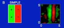
Figure 14: Computational modelling of a receptive field profile over the spatial domain in the primary visual cortex (V1) as reported by DeAngelis et al. [4, 5] using affine Gaussian derivatives: (middle) Receptive field profile of a simple cell over image intensities as reconstructed from cell recordings, with positive weights represented as green and negative weights by red. (left) Stylized simplification of the receptive field shape. (right) Idealized model of the receptive field from a first-order directional derivative of an affine Gaussian kernel $\partial_{x}g(x,y;\;\Sigma)=\partial_{x}g(x,y;\;\lambda_{x},\lambda_{y})$ according to (20), here with $\sigma_{x}=\sqrt{\lambda_{x}}=0.45$ and $\sigma_{y}=\sqrt{\lambda_{y}}=1.4$ in units of degrees of visual angle, and with positive weights with respect to image intensities represented by white and negative values by violet.

		$\partial_{\bot\varphi}g(x,y;\;\Sigma)$

Figure 15: Computational modelling of a spatio-chromatic receptive field profile over the spatial domain for a double-opponent simple cell in the primary visual cortex (V1) as measured by Johnson et al. [23] using affine Gaussian derivatives over a colour-opponent channel: (left) Responses to L-cones corresponding to long wavelength red cones, with positive weights represented by red and negative weights by blue. (middle) Responses to M-cones corresponding to medium wavelength green cones, with positive weights represented by red and negative weights by blue. (right) Idealized model of the receptive field from a first-order directional derivative of an affine Gaussian kernel $\partial_{\bot\varphi}g(x,y;\;\Sigma)$ according to (20) over a red-green colour-opponent channel for $\sigma_{1}=\sqrt{\lambda_{1}}=0.6$ and $\sigma_{2}=\sqrt{\lambda_{2}}=0.2$ in units of degrees of visual angle, $\alpha=67~{}\mbox{degrees}$ and with positive weights for the red-green colour-opponent channel represented by red and negative values by green.

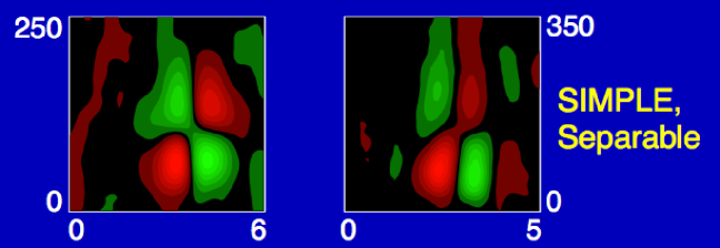
$h_{xt}(x,t;\;s,\tau)$	$-h_{xxt}(x,t;\;s,\tau)$

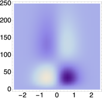
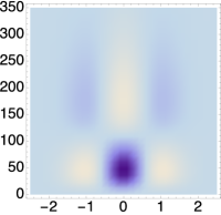
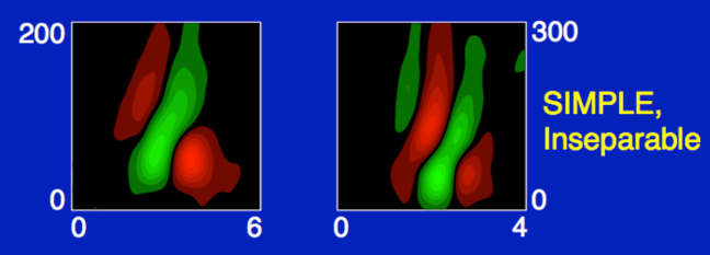
$h_{xx}(x,t;\;s,\tau,v)$	$-h_{xxx}(x,t;\;s,\tau,v)$

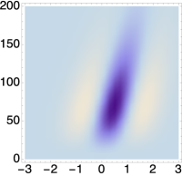
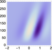
Figure 16: Computational modelling of simple cells in the primary visual cortex (V1) based on neural cell recordings reported by DeAngelis et al. [4] and using idealized spatio-temporal receptive fields of the form $T(x,t;\;s,\tau,v)=\partial_{x^{m}}\partial_{t^{n}}(g(x-vt;\;s)\,h(t;\;\tau))$ according to Equation (LABEL:eq-spat-temp-RF-model-der) and with the temporal smoothing function $h(t;\;\tau)$ modelled as a cascade of first-order integrators/truncated exponential kernels of the form (26): (upper part) Separable receptive fields corresponding to mixed derivatives of first- or second-order derivatives over space with first-order derivatives over time. (lower part) Inseparable velocity-adapted receptive fields corresponding to second- or third-order derivatives over space. Parameter values with $\sigma_{x}=\sqrt{s}$ and $\sigma_{t}=\sqrt{\tau}$: (a) $h_{xt}$: $\sigma_{x}=0.6$ degrees, $\sigma_{t}=60$ ms. (b) $h_{xxt}$: $\sigma_{x}=0.6$ degrees, $\sigma_{t}=80$ ms. (c) $h_{xx}$: $\sigma_{x}=0.7$ degrees, $\sigma_{t}=50$ ms, $v=0.007$ degrees/ms. (d) $h_{xxx}$: $\sigma_{x}=0.5$ degrees, $\sigma_{t}=80$ ms, $v=0.004$ degrees/ms. (Horizontal axis: Space $x$ in degrees of visual angle. Vertical axis: Time $t$ in ms.)

4.2 Double-opponent spatio-chromatic receptive fields in the LGN

In a study of spatio-chromatic response properties of V1 neurons in the alert macaque monkey, Conway and Livingstone [22] describe receptive fields with approximately circular red/green and yellow/blue colour-opponent response properties over the spatio-chromatic domain, see Figure 13. Such cells are referred to as double-opponent cells, since they simultaneously compute both spatial and chromatic opponency. According to Conway and Livingstone [22], this cell type can be regarded as the first layer of spatially opponent colour computations.

If we, motivated by the previous application of Laplacian of Gaussian functions to model rotationally symmetric on-center/off-surround and off-center/on-surround receptive fields in the LGN (38), apply the Laplacian of the Gaussian operator to red/green and yellow/blue colour-opponent channels,

$$\left(\begin{array}[]{c}f\\ u\\ v\end{array}\right)=\left(\begin{array}[]{ccc}\tfrac{1}{3}&\tfrac{1}{3}&\tfrac{1}{3}\\ \tfrac{1}{2}&-\tfrac{1}{2}&0\\ \tfrac{1}{2}&\tfrac{1}{2}&-1\\ \end{array}\right)\left(\begin{array}[]{c}R\\ G\\ B\end{array}\right),$$ (40)

respectively, we obtain equivalent spatio-chromatic receptive fields corresponding to red-center/green-surround, green-center/red-surround, yellow-center/blue-surround or blue-center/yellow-surround, respectively, as shown in Figure 13 and corresponding to the following spatio-chromatic receptive field model applied to the RGB channels

$$h_{double-opponent}(x,y;\;s)=\\ \pm(\partial_{xx}+\partial_{yy})\,g(x,y;\;s)\left(\begin{array}[]{ccc}\tfrac{1}{2}&-\tfrac{1}{2}&0\\ \tfrac{1}{2}&\tfrac{1}{2}&-1\\ \end{array}\right).$$ (41)

In this respect, these spatio-chromatic receptive fields can be used as an idealized model for the spatio-chromatic response properties for double-opponent cells.

4.3 Spatial, spatio-chromatic and spatio-temporal receptive fields in V1

Concerning the neurons in the primary visual cortex (V1), DeAngelis et al. [4, 5] describe that their receptive fields are generally different from the receptive fields in the LGN in the sense that they are (i) oriented in the spatial domain and (ii) sensitive to specific stimulus velocities. Cells (iii) for which there are precisely localized “on” and “off” subregions with (iv) spatial summation within each subregion, (v) spatial antagonism between on- and off-subregions and (vi) whose visual responses to stationary or moving spots can be predicted from the spatial subregions are referred to as simple cells (Hubel and Wiesel [1, 2, 3]).

Figure 15 shows an example of the spatial dependency of a simple cell, that can be well modelled by a first-order affine Gaussian derivative over image intensities. Figure 15 shows corresponding results for a color-opponent receptive field of a simple cell in V1, that can be modelled as a first-order affine Gaussian spatio-chromatic derivative over an R-G colour-opponent channel.

Figure 16 shows the result of modelling the spatio-temporal receptive fields of simple cells in V1 in this way, using the general idealized model of spatio-temporal receptive fields in Equation (LABEL:eq-spat-temp-RF-model-der) in combination with a temporal smoothing kernel obtained by coupling a set of truncated exponential kernels in cascade (26). The results in the upper part show space-time separable spatio-temporal receptive fields corresponding to zero image velocity $v=0$, and corresponding to either first- or second-order spatial derivatives over image space in combination with first-order temporal derivatives over time. The results in the lower part show inseparable spatio-temporal receptive fields corresponding to non-zero image velocities and based on either second- or third-order spatial derivatives over image space.

As can be seen from these figures, the proposed idealized receptive field models do quite well reproduce the qualitative shape of the neurophysiologically recorded biological receptive fields.

5 Relations to previous work

Young [30] has shown how spatial receptive fields in cats and monkeys can be well modelled by Gaussian derivatives up to order four. Young et al. [31, 32] have also shown how spatio-temporal receptive fields can be modelled by Gaussian derivatives over a spatio-temporal domain, corresponding to the Gaussian spatio-temporal concept described here, although with a different type of parameterization; see also [45, 46] for our closely related earlier work. The normative theory for visual receptive fields presented in [13, 19, 20, 21] and here does first of all provide additional theoretical foundation for Young’s spatial modelling work based on Koenderink and van Doorn’s theory [8, 9] and does additionally provide a conceptual extension to a time-causal spatio-temporal domain that takes into explicit account the fact that the future cannot be accessed. Additionally, our model provides a better parameterization of the spatio-temporal receptive field model over a non-causal spatio-temporal domain based on the Gaussian spatio-temporal scale-space concept.

This model or earlier versions of it has in turn been exploited for modelling of biological receptive fields by Lowe [47], May and Georgeson [48], Hesse and Georgeson [49], Georgeson et al. [50], Wallis and Georgeson [51], Hansen and Neumann [52], Wang and Spratling [53], Mahmoodi [54, 55] and Pei et al. [56].

5.1 Relations to modelling by Gabor functions

Gabor functions [57]

$$G(x;\;s,\omega)=e^{-i\omega x}\,g(x;\;s),$$ (42)

have been frequently used for modelling spatial receptive fields (Marčelja [24]; Jones and Palmer [25, 26]; Ringach [27, 28]) motivated by their property of minimizing the uncertainty relation. This motivation can, however, be questioned on both theoretical and empirical grounds. Stork and Wilson [58] argue that (i) only complex-valued Gabor functions that cannot describe single receptive field minimize the uncertainty relation, (ii) the real functions that minimize this relation are Gaussian derivatives rather than Gabor functions and (iii) comparisons among Gabor and alternative fits to both psychophysical and physiological data have shown that in many cases other functions (including Gaussian derivatives) provide better fits than Gabor functions do.

Conceptually, the ripples of the Gabor functions, which are given by complex sine waves, are related to the ripples of Gaussian derivatives, which are given by Hermite functions. A Gabor function, however, requires the specification of a scale parameter and a frequency, whereas a Gaussian derivative requires a scale parameter and the order of differentiation (per spatial and temporal dimension). With the Gaussian derivative model, receptive fields of different orders can be mutually related by derivative operations, and be computed from each other by nearest-neighbour operations. The zero-order receptive fields as well as the derivative based receptive fields can be modelled by diffusion equations, and can therefore be implemented by computations between neighbouring computational units.

In relation to invariance properties, the family of affine Gaussian kernels is closed under affine image deformations, whereas the family of Gabor functions obtained by multiplying rotationally symmetric Gaussians with sine and cosine waves is not closed under affine image deformations. This means that it is not possible to compute truly affine invariant image representations from such Gabor functions. Instead, given a pair of images that are related by a non-uniform image deformation, the lack of affine covariance implies that there will be a systematic bias in image representations derived from such Gabor functions, corresponding to the difference between the backprojected Gabor functions in the two image domains. If using receptive profiles defined from directional derivatives of affine Gaussian kernels, it will on the other hand be possible to compute affine invariant image representations [20], in turn providing better internal consistency between receptive field responses computed from different views of objects in the world.

With regard to invariance to multiplicative illumination variations, the even cosine component of a Gabor function does in general not have its integral equal to zero, which means that the illumination invariant properties under multiplicative illumination variations or exposure control mechanisms described in Section 3.4 do not hold for Gabor functions.

In this respect, the Gaussian derivative model is simpler, it can be related to image measurements by differential geometry, be derived axiomatically from symmetry principles, be computed from a minimal set of connections and allows for provable invariance properties under locally linearized image deformations (affine transformations) as well as local multiplicative illumination variations and exposure control mechanisms.

5.2 Relations to approaches for learning receptive fields from natural image statistics

Work has also been performed on learning receptive field properties and visual models from the statistics of natural image data (Field [59]; van der Schaaf and van Hateren [60]; Olshausen and Field [61]; Rao and Ballard [62]; Simoncelli and Olshausen [63]; Geisler [64]; Hyvärinen et al. [65]; Lörincz [66]) and been shown to lead to the formation of similar receptive fields as found in biological vision. The proposed theory of receptive fields can be seen as describing basic physical constraints under which a learning based method for the development of receptive fields will operate and the solutions to which an optimal adaptive system may converge to, if exposed to a sufficiently large and representative set of natural image data (see Figure 17).

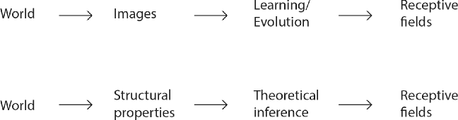
Figure 17: Two structurally different ways of deriving receptive field shapes for a vision system intended to infer properties of the world by either biological or artificial visual perception. (top row) A traditional model for learning receptive fields shapes consists of collecting real-world image data from the environment, and then applying learning algorithms possibly in combination with evolution over multiple generations of the organism that the vision system is a part of. (bottom row) With the normative theory for receptive fields presented in this paper, a short-cut is made in the sense that the derivation of receptive field shapes starts from structural properties of the world (corresponding to symmetry properties in theoretical physics) from which receptive field shapes are constrained by theoretical mathematical inference.

Field [59] as well as Doi and Lewicki [67] have described how ”natural images are not random, instead they exhibit statistical regularities” and have used such statistical regularities for constraining the properties of receptive fields. The theory presented in this paper can be seen as a theory at a higher level of abstraction, in terms of basic principles that reflect properties of the environment that in turn determine properties of the image data, without need for explicitly constructing specific statistical models for the image statistics. Specifically, the proposed theory can be used for explaining why the above mentioned statistical models lead to qualitatively similar types of receptive fields as the idealized functional models of receptive fields obtained from our theory.

An interesting observation that can be made from the similarities between the receptive field families derived by necessity from the assumptions and the receptive profiles found by cell recordings in biological vision, is that receptive fields in the retina, LGN and V1 of higher mammals are very close to ideal in view of the stated structural requirements/symmetry properties. In this sense, biological vision can be seen as having adapted very well to the transformation properties of the outside world and the transformations that occur when a three-dimensional world is projected to a two-dimensional image domain.

5.3 Logarithmic brightness scale

The notion of a logarithmic brightness scale goes back to the Greek astronomer Hipparchus, who constructed a subjective scale for the brightness of stars in six steps labelled “1 …6”, where the brightest stars were said to be of the first magnitude ($m=1$), while the faintest stars near the limits of human perception were of the sixth magnitude. Later, when quantitative physical measurements were made possible of the intensities of different stars, it was noted that Hipparchus subjective scale did indeed correspond to a logarithmic scale. In astronomy today, the apparent brightness of stars is still measured on a logarithmic scale, although extended over a much wider span of intensity values. A logarithmic transformation of image intensities is also used in the retinex theory (Land [68, 69]).

In psychophysics, the Weber-Fechner law attempts to describe the relationship between the physical magnitude and the perceived intensity of stimuli. This law states that the ratio of an increment threshold $\Delta I$ for a just noticeable difference in relation to the background intensity $I$ is constant over large ranges of magnitude variations [70, Pages 671–672]

$$\frac{\Delta I}{I}=k,$$ (43)

where the constant $k$ is referred to as the Weber ratio. The theoretical analysis of invariance properties of a logarithmic brightness scale under multiplicative transformations of the illumination field as well as multiplicative exposure control mechanisms in Section 3.4 is in excellent agreement with these psychophysical findings. If one considers an adaptive image exposure mechanism in the retina that adapts the diameter of the pupil and the sensitivity of the photopigments such that relative range variability in the signal divided by the mean illumination is held constant (43) (see e.g. Peli [71]), then such an adaptation mechanism can be seen as implementing an approximation of the derivative of a logarithmic transformation

$$d(\log z)=\frac{dz}{z}.$$ (44)

For a strictly positive entity $z$, there are also information theoretic arguments to regard $\log z$ as a default parameterization (Jaynes [72]). This property is essentially related to the fact that the ratio $dz/z$ then becomes a dimensionless integration measure. A general recommendation of care should, however, be taken when using such reasoning based on dimensionality arguments, since important phenomena could be missed, e.g., in the presence of hidden variables. The physical modelling of the effect of illumination variations on receptive field measurements in Section 3.4 provides a formal justification for using a logarithmic brightness scale in this context as well as an additional contribution of showing how the receptive field measurements can be related to inherent physical properties of object surfaces in the environment.

6 Summary

Neurophysiological cell recordings have shown that mammalian vision has developed receptive fields that are tuned to different sizes and orientations in the image domain as well as to different image velocities in space-time. A main message of this article has been to show that it is possible to derive such families of receptive field profiles by necessity, given a set of structural requirements on the first stages of visual processing as formalized into the notion of an idealized vision system, and whose functionality is determined by set of mathematical and physical assumptions (see Figure 17).

These structural requirements reflect structural properties of the world for the receptive fields to be compatible with natural image transformations including: (i) variations in the sizes of objects in the world, (ii) variations in the viewing distance, (iii) variations in the viewing direction, (iv) variations in the relative motion between objects in the world and the observer, (v) variations in the speed by which temporal events occur and (vi) local multiplicative illumination variations or multiplicative exposure control mechanisms, which are natural to adapt to for a vision system that is to interact with the world in a successful manner. In a competition between different organisms, adaptation to these properties may constitute an evolutionary advantage.

The presented theoretical model provides a normative theory for deriving functional models of linear receptive fields based on Gaussian derivatives and closely related operators. Specifically, the proposed theory can explain the different shapes of receptive field profiles that are found in biological vision from a requirement that the visual system should be able to compute covariant receptive field responses under the natural types of image transformations that occur in the environment, to enable the computation of invariant representations for perception at higher levels [20].

The presented theory leads to a computational framework for defining spatial and spatio-temporal receptive fields from visual data with the attractive properties that: (i) the receptive field profiles can be derived by necessity from first principles and (ii) it leads to predictions about receptive field profiles in good agreement with receptive fields found by cell recordings in biological vision. Specifically, idealized functional models have been presented for space-time separable receptive fields in the retina and the LGN and for both space-time separable and non-separable simple cells in the primary visual cortex (V1).

The qualitatively very good agreement between the predicted receptive field profiles from the normative axiomatic theory with the receptive field profiles found by neurophysiological measurements indicates that the earliest receptive fields in higher mammal vision have reached a state that can be seen as very close to ideal in view of the stated structural requirements/symmetry properties. In this sense, biological vision can be seen as having adapted very well to the transformation properties of the outside world and to the transformations that occur when a three-dimensional world is projected onto a two-dimensional image domain.

Compared to more common approaches of learning receptive field profiles from natural image statistics, the proposed framework makes it possible to derive the shapes of idealized receptive fields without any need for training data. The proposed framework for invariance and covariance properties also adds explanatory value by showing that the families of receptive profiles tuned to different orientations in space and image velocities in space-time that can be observed in biological vision can be explained from the requirement that the receptive fields should be covariant under basic image transformations to enable true invariance properties. If the underlying receptive fields would not be covariant, then there would be a systematic bias in the visual operations, corresponding to the amount of mismatch between the backprojected receptive fields.

Corresponding types of arguments applied to the area of hearing, lead to the formulation of a normative theory of auditory receptive fields (Lindeberg and Friberg [73, 74]).

References

- [1] D. H. Hubel and T. N. Wiesel, “Receptive fields of single neurones in the cat’s striate cortex,” J Physiol, vol. 147, pp. 226–238, 1959.
- [2] ——, “Receptive fields, binocular interaction and functional architecture in the cat’s visual cortex,” J Physiol, vol. 160, pp. 106–154, 1962.
- [3] ——, Brain and Visual Perception: The Story of a 25-Year Collaboration. Oxford University Press, 2005.
- [4] G. C. DeAngelis, I. Ohzawa, and R. D. Freeman, “Receptive field dynamics in the central visual pathways,” Trends in Neuroscience, vol. 18, no. 10, pp. 451–457, 1995.
- [5] G. C. DeAngelis and A. Anzai, “A modern view of the classical receptive field: Linear and non-linear spatio-temporal processing by V1 neurons,” in The Visual Neurosciences, L. M. Chalupa and J. S. Werner, Eds. MIT Press, 2004, vol. 1, pp. 704–719.
- [6] T. Iijima, “Observation theory of two-dimensional visual patterns,” Papers of Technical Group on Automata and Automatic Control, IECE, Japan, Tech. Rep., 1962.
- [7] A. P. Witkin, “Scale-space filtering,” in Proc. 8th Int. Joint Conf. Art. Intell., Karlsruhe, Germany, Aug. 1983, pp. 1019–1022.
- [8] J. J. Koenderink, “The structure of images,” Biological Cybernetics, vol. 50, pp. 363–370, 1984.
- [9] J. J. Koenderink and A. J. van Doorn, “Representation of local geometry in the visual system,” Biological Cybernetics, vol. 55, pp. 367–375, 1987.
- [10] ——, “Generic neighborhood operators,” IEEE Trans. Pattern Analysis and Machine Intell., vol. 14, no. 6, pp. 597–605, Jun. 1992.
- [11] T. Lindeberg, Scale-Space Theory in Computer Vision. Springer, 1993.
- [12] ——, “Scale-space theory: A basic tool for analysing structures at different scales,” Journal of Applied Statistics, vol. 21, no. 2, pp. 225–270, 1994, also available from http://www.csc.kth.se/tony/abstracts/Lin94-SI-abstract.html.
- [13] ——, “Generalized Gaussian scale-space axiomatics comprising linear scale-space, affine scale-space and spatio-temporal scale-space,” Journal of Mathematical Imaging and Vision, vol. 40, no. 1, pp. 36–81, 2011.
- [14] ——, “Generalized axiomatic scale-space theory,” in Advances in Imaging and Electron Physics, P. Hawkes, Ed. Elsevier, 2013, vol. 178, pp. 1–96.
- [15] L. M. J. Florack, Image Structure, ser. Series in Mathematical Imaging and Vision. Springer, 1997.
- [16] J. Sporring, M. Nielsen, L. Florack, and P. Johansen, Eds., Gaussian Scale-Space Theory: Proc. PhD School on Scale-Space Theory, ser. Series in Mathematical Imaging and Vision. Copenhagen, Denmark: Springer, 1997.
- [17] J. Weickert, S. Ishikawa, and A. Imiya, “Linear scale-space has first been proposed in Japan,” Journal of Mathematical Imaging and Vision, vol. 10, no. 3, pp. 237–252, 1999.
- [18] B. ter Haar Romeny, Front-End Vision and Multi-Scale Image Analysis. Springer, 2003.
- [19] T. Lindeberg, “A computational theory of visual receptive fields,” Biological Cybernetics, vol. 107, no. 6, pp. 589–635, 2013.
- [20] ——, “Invariance of visual operations at the level of receptive fields,” PLOS ONE, vol. 8, no. 7, p. e66990, 2013.
- [21] ——, “Time-causal and time-recursive spatio-temporal receptive fields,” Journal of Mathematical Imaging and Vision, vol. 55, no. 1, pp. 50–88, 2016.
- [22] B. R. Conway and M. S. Livingstone, “Spatial and temporal properties of cone signals in alert macaque primary visual cortex,” Journal of Neuroscience, vol. 26, no. 42, pp. 10 826–10 846, 2006.
- [23] E. N. Johnson, M. J. Hawken, and R. Shapley, “The orientation selectivity of color-responsive neurons in Macaque V1,” The Journal of Neuroscience, vol. 28, no. 32, pp. 8096–8106, 2008.
- [24] S. Marcelja, “Mathematical description of the responses of simple cortical cells,” Journal of Optical Society of America, vol. 70, no. 11, pp. 1297–1300, 1980.
- [25] J. Jones and L. Palmer, “The two-dimensional spatial structure of simple receptive fields in cat striate cortex,” J. of Neurophysiology, vol. 58, pp. 1187–1211, 1987.
- [26] ——, “An evaluation of the two-dimensional Gabor filter model of simple receptive fields in cat striate cortex,” J. of Neurophysiology, vol. 58, pp. 1233–1258, 1987.
- [27] D. L. Ringach, “Spatial structure and symmetry of simple-cell receptive fields in macaque primary visual cortex,” Journal of Neurophysiology, vol. 88, pp. 455–463, 2002.
- [28] ——, “Mapping receptive fields in primary visual cortex,” Journal of Physiology, vol. 558, no. 3, pp. 717–728, 2004.
- [29] R. W. Rodieck, “Quantitative analysis of cat retinal ganglion cell response to visual stimuli,” Vision Research, vol. 5, no. 11, pp. 583–601, 1965.
- [30] R. A. Young, “The Gaussian derivative model for spatial vision: I. Retinal mechanisms,” Spatial Vision, vol. 2, pp. 273–293, 1987.
- [31] R. A. Young, R. M. Lesperance, and W. W. Meyer, “The Gaussian derivative model for spatio-temporal vision: I. Cortical model,” Spatial Vision, vol. 14, no. 3, 4, pp. 261–319, 2001.
- [32] R. A. Young and R. M. Lesperance, “The Gaussian derivative model for spatio-temporal vision: II. Cortical data,” Spatial Vision, vol. 14, no. 3, 4, pp. 321–389, 2001.
- [33] A. Omurtag, B. W. Knight, and L. Sirovich, “On the simulation of large populations of neurons,” Journal of Computational Neuroscience, vol. 8, pp. 51–63, 2000.
- [34] M. Mattia and P. D. Guidice, “Population dynamics of interacting spiking neurons,” Physics Review E, vol. 66, no. 5, p. 051917, 2002.
- [35] O. Faugeras, J. Toubol, and B. Cessac, “A constructive mean-field analysis of multi-population neural networks with random synaptic weights and stochastic inputs,” Frontiers in Computational Neuroscience, vol. 3, no. 1, p. 10.3389/neuro.10.001.2009, 2009.
- [36] I. I. Hirschmann and D. V. Widder, The Convolution Transform. Princeton, New Jersey: Princeton University Press, 1955.
- [37] T. Lindeberg, “Temporal scale selection in time-causal scale space,” Journal of Mathematical Imaging and Vision, 2017, doi:10.1007/s10851-016-0691-3.
- [38] ——, “Scale-space for discrete signals,” IEEE Trans. Pattern Analysis and Machine Intell., vol. 12, no. 3, pp. 234–254, Mar. 1990.
- [39] T. Lindeberg and D. Fagerström, “Scale-space with causal time direction,” in Proc. European Conf. on Computer Vision (ECCV’96), ser. Springer LNCS, vol. 1064, Cambridge, UK, Apr. 1996, pp. 229–240.
- [40] T. Lindeberg, “Feature detection with automatic scale selection,” International Journal of Computer Vision, vol. 30, no. 2, pp. 77–116, 1998.
- [41] ——, “Edge detection and ridge detection with automatic scale selection,” International Journal of Computer Vision, vol. 30, no. 2, pp. 117–154, 1998.
- [42] ——, “Scale selection,” in Computer Vision: A Reference Guide, K. Ikeuchi, Ed. Springer, 2014, pp. 701–713.
- [43] ——, “Spatio-temporal scale selection in video data,” In preparation, 2017.
- [44] V. Bonin, V. Mante, and M. Carandini, “The suppressive field of neurons in the lateral geniculate nucleus,” The Journal of Neuroscience, vol. 25, no. 47, pp. 10 844–10 856, 2005.
- [45] T. Lindeberg, “Linear spatio-temporal scale-space,” in Proc. International Conference on Scale-Space Theory in Computer Vision (Scale-Space’97), ser. Springer LNCS, B. M. ter Haar Romeny, L. M. J. Florack, J. J. Koenderink, and M. A. Viergever, Eds., vol. 1252. Utrecht, The Netherlands: Springer, Jul. 1997, pp. 113–127.
- [46] ——, “Linear spatio-temporal scale-space,” Dept. of Numerical Analysis and Computer Science, KTH, Tech. Rep. ISRN KTH/NA/P–01/22–SE, Nov. 2001, available from http://www.csc.kth.se/cvap/abstracts/cvap257.html.
- [47] D. G. Lowe, “Towards a computational model for object recognition in IT cortex,” in Biologically Motivated Computer Vision, ser. Springer LNCS, vol. 1811. Springer, 2000, pp. 20–31.
- [48] K. A. May and M. A. Georgeson, “Blurred edges look faint, and faint edges look sharp: The effect of a gradient threshold in a multi-scale edge coding model,” Vision Research, vol. 47, no. 13, pp. 1705–1720, 2007.
- [49] G. S. Hesse and M. A. Georgeson, “Edges and bars: where do people see features in 1-D images?” Vision Research, vol. 45, no. 4, pp. 507–525, 2005.
- [50] M. A. Georgeson, K. A. May, T. C. A. Freeman, and G. S. Hesse, “From filters to features: Scale-space analysis of edge and blur coding in human vision,” Journal of Vision, vol. 7, no. 13, pp. 7–, 2007.
- [51] S. A. Wallis and M. A. Georgeson, “Mach edges: Local features predicted by 3rd derivative spatial filtering,” Vision Research, vol. 49, no. 14, pp. 1886–1893, 2009.
- [52] T. Hansen and H. Neumann, “A recurrent model of contour integration in primary visual cortex,” Journal of Vision, vol. 8, no. 8, pp. 8–, 2008.
- [53] Q. Wang and M. W. Spratling, “Contour detection in colour images using a neurophysiologically inspired model,” Cognitive Computation, vol. 8, no. 6, pp. 1027–1035, 2016.
- [54] S. Mahmoodi, “Linear neural circuitry model for visual receptive fields,” Journal of Mathematical Imaging and Vision, vol. 54, no. 2, pp. 1–24, 2016.
- [55] ——, “Nonlinearity in simple and complex cells in early biological visual systems,” Journal of Mathematical Imaging and Vision, pp. 1–10, 2017.
- [56] Z.-J. Pei, G.-X. Gao, B. Hao, Q.-L. Qiao, and H.-J. Ai, “A cascade model of information processing and encoding for retinal prosthesis,” Neural Regeneration Research, vol. 11, no. 4, p. 646, 2016.
- [57] D. Gabor, “Theory of communication,” J. of the IEE, vol. 93, pp. 429–457, 1946.
- [58] D. G. Stork and H. R. Wilson, “Do Gabor functions provide appropriate descriptions of visual cortical receptive fields,” Journal of Optical Society of America, vol. 7, no. 8, pp. 1362–1373, 1990.
- [59] D. J. Field, “Relations between the statistics of natural images and the response properties of cortical cells,” Journal of Optical Society of America, vol. 4, pp. 2379–2394, 1987.
- [60] A. van der Schaaf and J. H. van Hateren, “Modelling the power spectra of natural images: Statistics and information,” Vision Research, vol. 36, no. 17, pp. 2759–2770, 1996.
- [61] B. A. Olshausen and D. J. Field, “Emergence of simple-cell receptive field properties by learning a sparse code for natural images,” Journal of Optical Society of America, vol. 381, pp. 607–609, 1996.
- [62] R. P. N. Rao and D. H. Ballard, “Development of localized oriented receptive fields by learning a translation-invariant code for natural images,” Computation in Neural Systems, vol. 9, no. 2, pp. 219–234, 1998.
- [63] E. P. Simoncelli and B. A. Olshausen, “Natural image statistics and neural representations,” Annual Review of Neuroscience, vol. 24, pp. 1193–1216, 2001.
- [64] W. S. Geisler, “Visual perception and the statistical properties of natural scenes,” Annual Review of Psychology, vol. 59, pp. 10.1–10.26, 2008.
- [65] A. Hyvärinen, J. Hurri, and P. O. Hoyer, Natural Image Statistics: A Probabilistic Approach to Early Computational Vision, ser. Computational Imaging and Vision. Springer, 2009.
- [66] A. Lörincz, Z. Palotal, and G. Szirtes, “Efficient sparse coding in early sensory processing: Lessons from signal recovery,” PLOS Computational Biology, vol. 8(3), no. e1002372, 2012, 10.1371/journal.pcbi.1002372.
- [67] E. Doi and M. S. Lewicki, “Relations between the statistical regularities of natural images and the response properties of the early visual system,” in Japanese Cognitive Science Society: Sig P & P, Kyoto University, 2005, pp. 1–8.
- [68] E. H. Land, “The retinex theory of colour vision,” Proc. Royal Institution of Great Britain, vol. 57, pp. 23–58, 1974.
- [69] ——, “Recent advances in retinex theory,” Vision Research, vol. 26, no. 1, pp. 7–21, 1986.
- [70] S. E. Palmer, Vision Science: Photons to Phenomenology. MIT Press, 1999, first Edition.
- [71] E. Peli, “Contrast in complex images,” Journal of the Optical Society of America (JOSA A), vol. 7, no. 10, pp. 2032–2040, 1990.
- [72] E. T. Jaynes, “Prior probabilities,” Trans. on Systems Science and Cybernetics, vol. 4, no. 3, pp. 227–241, 1968.
- [73] T. Lindeberg and A. Friberg, “Idealized computational models of auditory receptive fields,” PLOS ONE, vol. 10, no. 3, pp. e0 119 032:1–58, 2015.
- [74] ——, “Scale-space theory for auditory signals,” in Proc. Scale-Space and Variational Methods for Computer Vision (SSVM 2015), ser. Lecture Notes in Computer Science, vol. 9087. Springer, 2015, pp. 3–15.