Invariant graphs of a family of non-uniformly expanding skew products over Markov maps

Abstract.

We consider a family of skew-products of the form $(Tx,g_{x}(t)):X\times\mathbb{R}\to X\times\mathbb{R}$ where $T$ is a continuous expanding Markov map and $g_{x}:\mathbb{R}\to\mathbb{R}$ is a family of homeomorphisms of $\mathbb{R}$. A function $u:X\to\mathbb{R}$ is said to be an invariant graph if $\mathrm{graph}(u)=\{(x,u(x))\mid x\in X\}$ is an invariant set for the skew-product; equivalently if $u(T(x))=g_{x}(u(x))$. A well-studied problem is to consider the existence, regularity and dimension-theoretic properties of such functions, usually under strong contraction or expansion conditions (in terms of Lyapunov exponents or partial hyperbolicity) in the fibre direction. Here we consider such problems in a setting where the Lyapunov exponent in the fibre direction is zero on a set of periodic orbits. We prove that $u$ either has the structure of a ‘quasi-graph’ (or ‘bony graph’) or is as smooth as the dynamics, and we give a criteria for this to happen.

1. Introduction and results

1.1. Introduction

Let $T$ be a continuous, expanding Markov map of the circle, $X$. Consider the skew product dynamical system $\tilde{T}_{g}:X\times\mathbb{R}\to X\times\mathbb{R}$ defined by

$$\tilde{T}_{g}(x,t)=(Tx,g(x,t)).$$ (1)

where $g(x,t):X\times\mathbb{R}\to\mathbb{R}$. A function $u:X\to\mathbb{R}$ is said to be an invariant graph if $\mathrm{graph}(u)=\{(x,u(x))\}$ is $\tilde{T}_{g}$-invariant; equivalently

$$u(Tx)=g(x,u(x)).$$ (2)

We refer to $X$ as the base and $\mathbb{R}$ as the fibre. We are interested in the case when $g(x,\cdot):\mathbb{R}\to\mathbb{R}$ is a homeomorphism; we normally write $g_{x}(t)=g(x,t)$, $g_{x}:\mathbb{R}\to\mathbb{R}$ and refer to $g_{x}(\cdot)$ as a skewing function. When $g_{x}$ is uniformly expanding, the invariant graph exists, is Hölder continuous and, under a partial hyperbolicity assumption, generically has no higher regularity. As a particular example, let $b\geq 2,b\in\mathbb{N}$ and let $Tx=bx\bmod 1$. Let $\lambda\in(0,1)$, $\lambda b>1$, and let $g_{x}(t)=\cos(2\pi x)+\lambda^{-1}t$. In this case the invariant graph $u(x)=-\sum_{n=0}^{\infty}\lambda^{n}\cos 2\pi b^{n}x$, the classical Weierstrass function.

More generally, if the Lyapunov exponent in the fibre direction is positive with respect to a given reference measure, then the invariant graph is measurable, (2) holds almost everywhere, and generically is not continuous [Sta99, HNW02]. Note that [HNW02] requires a partial hyperbolicity assumption on the skew-product.

In this note, we alter the non-uniform contraction condition in the fibre and assume that the Lyapunov exponent in the fibre direction is zero for certain measures. In particular, we consider the case when the skewing function is the identity map on a given set of periodic orbits. We construct a family of measurable invariant sets for the skew product and identify the set of measure zero on which (2) fails. Our invariant sets are generically almost everywhere graphs of functions that are discontinuous on every open set and are almost everywhere uniformly bounded.

We describe the precise structure of the invariant sets. The following dichotomy holds: either the invariant set is of a discontinuous nature of the form described above or is as smooth as the dynamics. The former case is generic; in this case (together with a partial hyperbolicity assumption) we also calculate the box dimension of the invariant set in terms of thermodynamic formalism.

The invariant sets we obtain are an example of a family of so-called bony attractors—a bony attractor is a closed set that intersects every almost every fibre at a single point and any other fibre at an interval. These sets were first described by [Kud10] and other examples occur in [KV14, GH16] as attractors of step functions over shift maps.

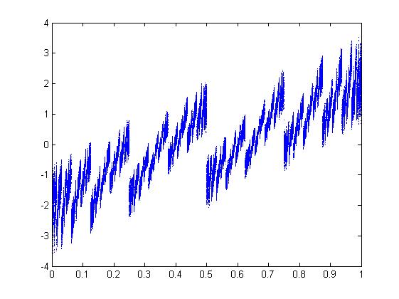
(a) An invariant graph defined on $X\setminus R_{P}$.

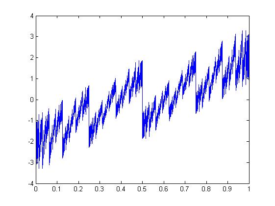
(b) The quasi-graph invariant set.

Figure 1. The invariant graph and an invariant set (quasi-graph) of the affine real-valued skew product $\tilde{T}_{g}(x,t)=(Tx,\sin(2\pi x)+\gamma^{-1}(x)t)$, where $\gamma(x)=\frac{3+\cos(2\pi x)}{4}$ and where $T$ is the doubling map. The skew product is the identity at the fixed point $x=0$ and the invariant graph is discontinuous at all pre-images of $0$.

1.2. Results

Let $\tilde{T}_{g}$ be a skew product as defined in (1). We write $g(x,t)=g_{x}(t)$ and assume that, for each $x\in X$, $g_{x}:\mathbb{R}\to\mathbb{R}$ is a homeomorphism. We also assume that, for each $t\in\mathbb{R}$, $x\mapsto g_{x}(t)$ is $\alpha$-Hölder continuous. We define $g^{n}_{x}(t)=g_{T^{n-1}x}g_{T^{n-2}x}\cdots g_{x}(t)$ so that $\tilde{T}_{g}^{n}(x,t)=(T^{n}x,g^{n}_{x}(t))$. We define $h_{x}(t)=g_{x}(t)^{-1}$ so that $g^{n}_{x}(t)^{-1}=h^{n}_{x}(t)=h_{x}\cdots h_{T^{n-1}x}(t)$. Let $P:=\bigcup_{r=0}^{\rho-1}P_{r}\subset X$ be a collection of $\rho$ distinct periodic orbits for $T:X\to X$. For $p\in P$ we denote by $\ell(p)$ the least period of $p$. Let $R_{P}$ be the set of pre-images of points in $P$; that is

$$R_{P}=\{x\in X\mid T^{n}x\in P\text{ for some }n\geq 0\}.$$

Note that this is a countable set. We will often consider the set $R_{P}$ and its complement $X\setminus R_{P}$ separately; both sets are $T$-invariant.

If $h_{x}:\mathbb{R}\to\mathbb{R}$ is a diffeomorphism, we define the derivative in the fibre direction to be

$$\partial h_{x}(t)=\lim_{\epsilon\to 0}\frac{h_{x}(t+\epsilon)-h_{x}(t)}{\epsilon}.$$

In §1.3 we will precisely define a set of skew products $\tilde{T}_{g}\in\mathcal{S}(X,\mathbb{R},C^{\alpha}_{P})$ where $\tilde{T}_{g}$ is expanding in the fibre direction except along the periodic orbits in $P$ where $g^{\ell(p)}_{p}(t)=t$ for all $t\in\mathbb{R}$. We shall abuse notation slightly and write $g\in C^{\alpha}_{P}$.

Remark 1.1.

Examples of skew products that satisfy our hypotheses include affine maps $g_{x}(t)=f(x)+\gamma(x)^{-1}t$ where $f$, $\gamma$ are $\alpha$-Hölder with $\gamma(p)=1$, $f(p)=0$ for $p\in P$ and otherwise $0<\gamma(x)<1$. Our conditions remain satisfied for diffeomorphisms $g:X\to\text{Diff}(\mathbb{R},\mathbb{R})$ defined by small, sufficiently smooth perturbations of affine maps preserving conditions (6) to (9) below. Figure 1 shows an explicit example.

First, we show that such invariant graphs exist. We prove that we have a unique invariant function $u$ on $X\setminus R_{P}$; hence the graph of this function is an invariant set of the restricted skew product $\tilde{T}_{g}|_{X\setminus R_{P}}$.

Theorem 1.

Let $\tilde{T}_{g}\in\mathcal{S}(X,\mathbb{R},C^{\alpha}_{P})$. There exists a uniformly bounded function $u:X\setminus R_{P}\to\mathbb{R}$ such that $u(Tx)=g_{x}(u(x))$ for $x\in X\setminus R_{P}$. Any other uniformly bounded function $v:X\setminus R_{P}\to\mathbb{R}$ satisfying this equation is equal to $u$; moreover, if $\mu$ is an ergodic measure for $T$ not supported on $R_{P}$, then $u$ is $\mu$-a.e. unique amongst the set of measurable functions.

We prove the following corollary to Theorem 1, showing that $u$ is uniquely defined on $X\setminus R_{P}$ but can be arbitrarily defined on $R_{P}$.

Corollary 2.

Let $\tilde{T}_{g}\in\mathcal{S}(X,\mathbb{R},C^{\alpha}_{P})$ and let $u$ be as in Theorem 1. Suppose that $P$ consists of $\rho$ periodic orbits. For each $r$ such that $0\leq r\leq\rho-1$, choose one element of each periodic orbit $p\in P_{r}\subset P$. There is a $\rho$-parameter family of invariant graphs for the skew product, $u_{s}:X\to\mathbb{R}$, where $u_{s}(p)=s_{r}$ for $s=(s_{0},\dots,s_{\rho-1})\in\mathbb{R}^{\rho}$. Furthermore, $u_{s}|_{X\setminus R_{P}}=u$.

Clearly, for $x\in R_{P}$, each fibre $\{x\}\times\mathbb{R}$ is $\tilde{T}_{g}$-invariant; by taking the union we have a dense $\tilde{T}_{g}$-invariant set. As $X\setminus R_{P}$ is dense in $X$, we can consider a sequence $x_{0}\to x$ for any $x\in R_{P}$ where each point $x_{0}\in X\setminus R_{P}$.

Definition 1.2.

Let $\tilde{T}_{g}\in\mathcal{S}(X,\mathbb{R},C^{\alpha}_{P})$. Define the invariant quasi-graph $U\subset X\times\mathbb{R}$ as $U=\bigcup_{x\in X}U_{x}$ where

$$U_{x}=\begin{cases}(x,u(x))&\text{ if }x\in X\setminus R_{P},\\ \{x\}\times[\liminf_{y\in X\setminus R_{P},y\to x}u(y),\limsup_{y\in X\setminus R_{P},y\to x}u(y)]&\text{ if }x\in R_{P}.\end{cases}$$

In other words, we connect the discontinuities between the values of the function $u$ as we approach $R_{P}$; see Figure 1. Denote the length of the interval of the quasi-graph at $x\in R_{P}$ by

$$|U_{x}|=\left|\limsup_{y\in X\setminus R_{P},y\to x}u(y)-\liminf_{y\in X\setminus R_{P},y\to x}u(y)\right|;$$

if $x\in X\setminus R_{P}$ then we set $|U_{x}|=0$. In Proposition 4.1 we show that $U$ is a $\tilde{T}_{g}$-invariant set.

We prove two main results about quasi-graphs, reminiscent of those found in the studies of Weierstrass functions, [Bar15, HL93] and for dynamically-defined invariant graphs [Sta99, HNW02]. The first is a dichotomy of the structure of the invariant graphs.

Theorem 3.

Let $\tilde{T}_{g}\in\mathcal{S}(X,\mathbb{R},C^{\alpha}_{P})$. Then either:

1. the invariant quasi-graph $U$ is the graph of a uniformly $\alpha$-Hölder continuous function;

2. for every $x\in R_{P}$, $|U_{x}|>0$.

When we are in the second case, we will often say “the quasi-graph $U$ is not the graph of an invariant function”. As $R_{P}$ is dense in $X$, we see that $U$ is not the graph of a function on any open set and has a ‘vertical jump’ at each element of $R_{P}$. It is easy to construct examples of continuous invariant graphs, but our second result proves that generically $U$ is of the discontinuous type.

Theorem 4.

Let $\tilde{T}_{g}\in\mathcal{S}(X,\mathbb{R},C^{\alpha}_{P})$. There exists a $C^{\alpha}$-open and $C^{0}$-dense set of $g\in C^{\alpha}_{P}$ such that the invariant quasi-graph $U$ of $\tilde{T}_{g}$ is not the graph of a function.

For higher regularity of $u$, we need higher regularity on the base dynamics $T$ and we consider $C^{r+\alpha}$-expanding endomorphisms of the circle, with $r\in\mathbb{N}$, $r\geq 1$ and $\alpha>0$. We also assume that that $g_{x}:\mathbb{R}\to\mathbb{R}$ is $C^{r+\alpha}$ and, for each $t$, $x\mapsto g_{x}(t)$ is $C^{r+\alpha}$. Again, we abuse notation slightly and write $g\in C^{r+\alpha}_{P}$. Denote this set of skew products by $\tilde{T}_{g}\in\mathcal{S}_{C^{r+\alpha}}(X,\mathbb{R},C^{r+\alpha}_{P})$. In this case we can strengthen the above dichotomy: if $U$ is the graph of a function then it is as smooth as the dynamics.

Theorem 5.

Let $\alpha\geq 0$, $r\in\mathbb{N}$ and $r\geq 1$. Let $\tilde{T}_{g}\in\mathcal{S}_{C^{r+\alpha}}(X,\mathbb{R},C^{r+\alpha}_{P})$. Then either:

1. the invariant quasi-graph $U$ is the graph of a $C^{r+\alpha}$ function;

2. for every $x\in R_{P}$, $|U_{x}|>0$.

Our final result concerns the box dimension of the invariant quasi-graphs. Our result extends that in [Bed89] to our setting, and we believe it is the first attempt to calculate the dimension of invariant graphs of non-uniformly expanding skew products. The key difficulty is establishing a sufficiently strong form of bounded distortion.

Let $q:X\to\mathbb{R}$ be a function and let $\mathfrak{m}(q)=\inf_{x\in X}q(x)$. Suppose $\partial g_{x}(t)>0$; we will show in Remark 3.2 that this causes no loss in generality. A skew product is partially hyperbolic if there exists $\kappa>1$ such that

$$1<\kappa\leq\mathfrak{m}(\partial h)\mathfrak{m}(|T^{\prime}|)$$ (3)

where the infimum $\mathfrak{m}(\partial h)$ is taken over all $(x,t)\in X\times\mathbb{R}$ and $h_{x}=g_{x}^{-1}$.

Suppose that $g:X\to C^{2}(\mathbb{R},\mathbb{R})$ is a $C^{2}$ diffeomorphism and we return to allowing $T:X\to X$ to be a continuous expanding Markov map (with conditions specified in §1.3). Let $x\mapsto h_{x}t$, $x\mapsto\partial h_{x}(t)$ and $x\mapsto\partial^{2}h_{x}(t)$ be Lipschitz continuous. Denote this set of skew products by $\mathcal{S}(X,\mathbb{R},C^{\operatorname{Lip},2}_{P})\subset\mathcal{S}(X,\mathbb{R},C^{\alpha}_{P})$.

Define the function

$$\mathcal{D}h(x)=\begin{cases}\partial h_{x}(u(Tx))&\text{ for }x\in X\setminus R_{P},\\ \partial h_{x}(t)&\text{ for }x\in R_{P},\text{ where }t=\limsup_{y\in X\setminus R_{P},y\to Tx}u(y).\end{cases}$$

Let $\mathcal{P}(\phi)$ be the topological pressure of a function $\phi:X\to\mathbb{R}$, see Definition 7.12. We prove the following.

Theorem 6.

Let $\tilde{T}_{g}\in\mathcal{S}(X,\mathbb{R},C^{\operatorname{Lip},2}_{P})$ be partially hyperbolic such that the invariant quasi-graph is not the graph of a continuous function on $X$. The box dimension of the quasi-graph $U$ is the unique solution $t$ to the generalised Bowen equation

$$\mathcal{P}((1-t)\log|T^{\prime}|+\log|\mathcal{D}h|)=0.$$ (4)

As $\partial h_{x}(t)$, and so $\mathcal{D}h(x)$, are uniformly bounded for $(x,t)\in X\times\mathbb{R}$, it is well-known that a unique solution to such an equation for a partially-hyperbolic skew-products exists and often corresponds to the dimension of graphs [Bed89, MW12].

1.3. The family of skew products

Here we list the technical hypotheses on the dynamics. We assume that $T$ is a $C^{1}$ expanding Markov map. Specifically, there is a partition $X=\bigcup_{j=0}^{b-1}X_{j}$, $X_{j}=[t_{j},t_{j+1}]$ with $0=t_{0}<t_{1}<\cdots<t_{b}=1$, such that, for each $j$, $T|_{X_{j}}:\mathop{\mathrm{Int}}X_{j}\to\bigcup_{i\in I_{j}}X_{i}$ is a $C^{1}$ diffeomorphism. We assume that $T$ is continuous. We assume there exists $\theta<1$ such that $|T^{\prime}(x)|\geq\theta^{-1}>1$ for all $x\in\bigcup_{i=0}^{b-1}\text{Int}(X_{j})$. We assume that $T$ is locally eventually onto, namely that there exists $N\in\mathbb{N}$ such that, for all $X_{j}$, $T^{N}X_{j}=X$ (equivalently, $T^{N}$ is full branched for some $N\in\mathbb{N}$). As $T|_{X_{j}}$ is a diffeomorphism onto its image, there exists a well-defined inverse branch $\omega_{j}:\bigcup_{i\in I_{j}}X_{i}\to X_{j}$ and $\omega_{j}$ is a diffeomorphism. Note that $d(\omega_{j}x,\omega_{j}y)\leq\theta d(x,y)$. Define a cylinder of rank $n$ by $C_{n}=C_{j_{0}j_{1}\dots j_{n-1}}=\omega_{j_{0}}\omega_{j_{1}}\dots\omega_{j_{n-1}}(X)$. Note that $C_{n}\subset X$ is an interval.

We now state the hypotheses on the skewing function. Let $P=\bigcup_{r=0}^{\rho-1}P_{r}$ be a finite set of periodic orbits. If $p\in P_{r}$ then we write $\ell(p)$ for the least period of $p$. Recall $h_{x}(t)=g_{x}(t)^{-1}$.

Fix a constant $C_{\mathcal{S}}\geq 1$. Suppose the skewing function $g$ is such that

$$g^{\ell(p)}_{p}(t)=t,$$ (5)

for all $t\in\mathbb{R}$ and $p\in P$. Suppose that

$$|h^{n}_{x}(t)-h^{n}_{x}(t^{\prime})|\leq C_{\mathcal{S}}|t-t^{\prime}|$$ (6)

for all $x\in X$. Let $\epsilon>0$ be small. Define the collection of open balls (intervals) in $X$ of radius $\epsilon$ centred on $p\in P$ by $B_{\epsilon}(P)=\bigcup_{p\in P}B_{\epsilon}(p)$ and let $G=X\backslash B_{\epsilon}(P)$. For an orbit segment $x,\dots,T^{n-1}x\in B_{\epsilon}(P)$, denote $\epsilon_{j}=\inf_{p\in P}d(T^{j}x,p)$. Suppose we can define a function $\lambda:[0,\epsilon]\to\mathbb{R}^{+}$ where $\log\lambda$ is $\alpha$-Hölder for some $\alpha>0$, with $\lambda(\epsilon)>0$ and $\lambda(0)=1$ such that

$$|h^{n}_{x}(t)-h^{n}_{x}(t^{\prime})|\geq C_{\mathcal{S}}^{-1}\lambda(\epsilon_{0})\dots\lambda(\epsilon_{n-1})|t-t^{\prime}|.$$ (7)

Let $\delta$ be such that $0<\delta\leq\epsilon$. Suppose that the orbit segment $x,\dots,T^{n-1}x$ visits $X\backslash B_{\delta}(P)$ $j$-many times, let there exist $0<\lambda_{\delta}<1$ such that

$$|h^{n}_{x}(t)-h^{n}_{x}(t^{\prime})|\leq C_{\mathcal{S}}\lambda_{\delta}^{j}|t-t^{\prime}|,$$ (8)

where $\lambda_{\delta}$ is independent of $x$, $t$ and $t^{\prime}$. We also assume that both $x\mapsto g_{x}(t)$ and $x\mapsto h_{x}(t)$ are $\alpha$-Hölder continuous,

$$|g_{x}(t)-g_{y}(t)|\leq C_{g}(t)d(x,y)^{\alpha}\hskip 14.22636pt\text{ and }\hskip 14.22636pt|h_{x}(t)-h_{y}(t)|\leq C_{h}(t)d(x,y)^{\alpha},$$ (9)

for some $\alpha>0$. If $t\in W$ and $W\subset\mathbb{R}$ is compact, then define $C_{W}=\sup_{t\in W}\{C_{g}(t),C_{h}(t)\}$.

As $x\mapsto g_{x}(t)$ is continuous and $X$ is compact, there exists $K_{g}>0$ independent of $x$ such that

$$|g^{n}_{x}(t)|\leq\sup_{0\leq j\leq n}\sup_{x\in X}|g^{n}_{x}(t)|=K_{g}(t,n).$$ (10)

Finally, as $g$ is invertible and continuous, there exists $\lambda_{\min}>0$ such that

$$|h^{n}_{x}(t)-h^{n}_{x}(t^{\prime})|\geq C^{-1}_{\mathcal{S}}\lambda_{\min}^{n}|t-t^{\prime}|.$$ (11)

Let $T:X\to X$ be a continuous, expanding, locally eventually onto Markov map. We denote the set of skew products of the form (1) satisfying conditions (5) to (9) with fixed constant $C_{\mathcal{S}}$ by $\mathcal{S}(X,\mathbb{R},C^{\alpha}_{P})$.

Remark 1.3.

Suppose $g_{x}(t)=f(x)+\gamma^{-1}(x)t$ as in Remark 1.1, where $\sum_{i=0}^{\ell(p)}f(T^{i}p)=0$, $0<\gamma(x)\leq 1$ and $\gamma(p)=1$ if and only if $p\in P$. The function $\lambda:[0,\epsilon]\to\mathbb{R}^{+}$ in condition (7) can be defined as $\lambda(\epsilon_{x})=|\gamma(x)|$ for $x\in B_{\epsilon}(P)$ where $\epsilon_{x}=\inf_{p\in P}d(x,p)$. In this case, for $\delta\leq\epsilon$, $\lambda_{\delta}$ in condition (8) is chosen as $\sup_{x\not\in B_{\delta}(P)}|\gamma(x)|<1$; also $\lambda_{\min}=\mathfrak{m}(|\gamma|)$.

For these skew products, the constant $C_{\mathcal{S}}=1$. Allowing the constant to be larger than $1$ allows $|\gamma(x)|>1$ at some $x\in X$ provided that $|\gamma^{n}(x)|<C_{\mathcal{S}}$ for all $n$, hence the Lyapunov exponent is non-positive. Throughout, we fix the constant $C_{\mathcal{S}}$ as, when we make a small perturbation of the skew product, the constant does not necessarily perturb independent of $n$. This is important in the proof of Theorem 4.

More generally, for $g_{x}$ a diffeomorphism with $0<\lambda_{\min}\leq|\partial h_{x}(t)|<1$ for $x\not\in P$ and $h^{\ell(p)}_{p}(t)=t$ if and only if $p\in P$, we define $\lambda(\epsilon_{x})=\mathfrak{m}(|\partial h_{x}|)$ and $\lambda_{\delta}=\sup_{x\not\in B_{\delta}(P)}\|\partial h_{x}\|_{\infty}$.

Remark 1.4.

Notice, unlike [Bed89] and [HNW02] we have no partial hyperbolicity condition in general.

Remark 1.5.

Suppose that the skewing function is not the identity over the periodic orbits of $P$ but has zero Lyapunov exponent. Say $g_{x}(t)=f(x)+\gamma(x)^{-1}t$, where $\gamma^{\ell}(p)=1$ but $f(p)>0$ for $p\in P$. In this setting, it is easy to see that the invariant graph is unbounded on pre-images of $P$. In fact, the two basins (of points repelled to $\pm\infty$) appear intermingled in the sense of [AYYK92, AP11, Kel15].

Remark 1.6.

For Theorem 1 and Corollary 2 we do not need $T$ to be locally eventually onto, rather just continuous and expanding.

2. Properties of Markov maps

To prove Theorem 1, we will need the following technical lemma. The content of the lemma is surely well-known, but we include a proof for completeness.

Lemma 2.1.

Let $T:X\to X$ be a continuous expanding Markov map of the circle. Let $p$ be a periodic point and let $P$ denote the periodic orbit of $p$. There exists $\epsilon>0$ such that for all $\delta$ where $0<\delta\leq\epsilon$ if the orbit sequence $\{x,Tx,\dots,T^{n}x\}\subset B_{\delta}(P)$ with $x\in B_{\delta}(p)$, then $d(T^{j}x,T^{j}p)<\delta\theta^{n-j}$ for all $0\leq j\leq n$.

Proof.

If $x=p$, then, as $P$ is $T$-invariant, the result is trivial.

We first prove that if $x\in B_{\delta}(p)$ and $Tx\in B_{\delta}(P)$, then $Tx\in B_{\delta}(Tp)$. Let $t_{j}$ be the lower end-point of the interval $X_{j}$. Let $Q=P\cup\{t_{i}\}_{i=0}^{b-1}$. Let $d=\inf_{q_{i}\not=q_{j}\in Q}d(q_{i},q_{j})$. Choose $\epsilon<d/\|T^{\prime}\|_{\infty}4$ and let $0<\delta\leq\epsilon$. As $\|T\|_{\infty}>1$, $\delta<d/4$ and so for $p\in P$ the balls $B_{\delta}(p)$ are pairwise disjoint.

For $x\not=p$, $x$ is located in precisely one of $(p-\delta,p)$ or $(p,p+\delta)$ and on these sets $T$ is differentiable (note, $p$ could be equal to $t_{j}$ for some $j$, hence we split the interval $B_{\delta}(p)$ at $p$). By the Mean Value Theorem, $d(Tx,Tp)\leq\|T^{\prime}\|_{\infty}d(x,p)<d/4$. Hence the set $T(B_{\delta}(p))$ has diameter at most $d/2$ and

$$T(B_{\delta}(p))\subset B_{d/2}(Tp).$$ (12)

By assumption, $Tx\in B_{\delta}(P)$. We show that $Tx\in B_{\delta}(Tp)$. Suppose not, say $Tx\in B_{\delta}(p^{\prime})$ with $p^{\prime}\in P$, $p^{\prime}\not=Tp$. Then $Tx\in B_{\delta}(p^{\prime})\cap T(B_{\delta}(p))$. By (12), $Tx\in B_{d/2}(p^{\prime})\cap B_{d/2}(Tp)$, contradicting that the points of $P$ are at least distance $d$ apart. So $Tx\in B_{\delta}(Tp)$.

Suppose that $p\in\text{Int}(X_{j})$ for some $j$; therefore $\omega_{j}(Tp)=p$. By choice of $\delta$, $T:B_{\delta}(x)\to X$ is a diffeomorphism on $B_{\delta}(x)\subset X_{j}$. Therefore, the inverse branch $\omega_{j}:T(B_{\delta}(x))\to X_{j}$ is a diffeomorphism on $T(B_{\delta}(x))$. As $T$ is expanding, $T(B_{\delta}(p))\supset B_{\delta}(Tp)$. By the Mean Value Theorem, for $x\in B_{\delta}(p)$,

$$\theta\geq\frac{d(\omega_{j}(Tx),\omega_{j}(Tp))}{d(Tx,Tp)}=\frac{d(x,p)}{d(Tx,Tp)}.$$ (13)

As $Tx\in B_{\delta}(Tp)$, we have $d(Tx,Tp)<\delta$ and so $d(x,p)<\theta\delta$.

Finally, consider the case where $p$ is the unique point of intersection $p\in X_{j-1}\cap X_{j}$. Then $\omega_{j}(Tp)=p=\omega_{j-1}(Tp)$. Either $x\in(p-\epsilon,p)\subset X_{j-1}$ or $x\in(p,p+\epsilon)\subset X_{j}$. In either case, by applying the appropriate inverse branch, the result follows by the idea of (13) above, replacing the ball $B_{\delta}(p)$ with intervals $(p,p+\epsilon)$ or $(p-\epsilon,p)$. By iterating this argument, if $T^{j}x\in B_{\delta}(P)$ for all $0\leq j\leq n$, then $d(T^{j}x,T^{j}p)<\delta\theta^{n-j}$, as required. ∎

The following corollary is also well-known: the only orbit that $\delta$-shadows a periodic orbit (for $\delta$ sufficiently small) is the periodic orbit itself.

Corollary 2.2.

Let $\delta>0$ be as in Lemma 2.1. Suppose for all $n\in\mathbb{N}$ we have $T^{n}x\in B_{\delta}(P)$. Then $x\in P$.

Proof.

Suppose $x\not\in P$. There exists $\eta>0$ such that, for all $p\in P$, $d(x,p)>\eta$. As $T^{n}x\in B_{\delta}(P)$ for all $n\in\mathbb{N}$, for any $m\in\mathbb{N}$ the orbit segment $\{x,\dots,T^{m}x\}\subset B_{\delta}(P)$. By Lemma 2.1, for some $p\in P$, we have $d(x,p)<\delta\theta^{m}$. Choose $m$ large such that $\delta\theta^{m}<\eta$, contradicting our assumption that $x\not\in P$. ∎

In order to prove the existence of an invariant graph, we show that $h^{n}_{x}(t)\to u(x)$. In our setting, when $x$ is very close to $P$, the rate of contraction of $h_{x}(t)$ is not uniformly bounded below $1$. Thus, supposing that the orbit segment $Tx,\dots,T^{n-1}x$ remains in $B_{\delta}(P)$, the next result uses Lemma 2.1 to bound $h^{n}_{x}(t)$ independently of $x$ and $n$.

Lemma 2.3.

Let $T:X\to X$ be a continuous expanding Markov Map of the interval. Let $0<\delta\leq\epsilon<1$ be as in Lemma 2.1. Let $g\in C^{\alpha}_{P}$. Let $n\geq 2$. If the orbit segment $\{Tx,\dots,T^{n-1}x\}$ lies in $B_{\delta}(P)$, then $|h^{n}_{x}(t)-t|\leq A_{h}(t)$, where $A_{h}(t)>0$ is independent of $n$ and $x$, but not $t$.

Proof.

Let $\ell$ be the least period of $p\in P$. Let $Tx\in B_{\delta}(Tp)$. Let $n_{\ell}$ be the smallest integer $n_{\ell}\geq n$ divisible by $\ell$, so $h^{n_{\ell}}_{p}(t)=(t)$ and $n_{\ell}-n\leq\ell-1$

As $\{Tx,\dots,T^{n-1}x\}\subset B_{\delta}(P)$, by Lemma 2.1, for $0\leq i\leq n-2$, $d(T^{i}(Tx),T^{i}(Tp))\leq\theta^{n-2-i}\delta$. Let $T^{n_{\ell}-n}q=p$. As $h^{n_{\ell}}_{q}$ is the identity,

$$|h^{n}_{x}(t)-t| =|h^{n}_{x}(t)-h^{n_{\ell}}_{q}(t)|\leq|h^{n}_{x}(t)-h^{n}_{p}(t)|+|h^{n}_{p}(t)-h^{n}_{p}(h^{n_{\ell}-n}_{q}(t))|.$$ (14)

We bound the first term of (14). By (6) and Lemma 2.1,

$$|h^{n}_{x}(t)-h^{n}_{p}(t)| \leq\sum_{i=0}^{n-1}|h^{i}_{x}h_{T^{i}x}h^{n-1-i}_{T^{i+1}p}(t)-h^{i}_{x}h_{T^{i}p}h^{n-1-i}_{T^{i+1}p}(t)|$$

$$\leq C_{\mathcal{S}}C_{g}(h^{n-1-i}_{T^{i+1}p}(t))\sum_{i=0}^{n-1}d(T^{i}x,T^{i}p)^{\alpha}$$

$$\leq C_{\mathcal{S}}C_{g}(h^{n-1-i}_{T^{i+1}p}(t))\left(1+\sum_{i=0}^{n-2}\theta^{\alpha(n-2-i)}\delta\right)\leq C(\ell,t).$$

as $h^{n-1-i}_{T^{i+1}p}(t)\in[-K_{g}(\ell,t),K_{g}(\ell,t)]=:W$, the Hölder constant $C_{g}(h^{n-1-i}_{T^{i+1}p}(t))<C_{W}$. We bound the second term of (14) by

$$|h^{n}_{p}(t)-h^{n}_{p}(h^{n_{\ell}-n}_{q}(t))| \leq C_{\mathcal{S}}|t-h^{n_{\ell}-n}_{q}(t)|\leq C_{\mathcal{S}}(|t|+K_{g}(t,\ell))$$

as $n_{\ell}-n\leq\ell$. Hence, we have the bound as required. ∎

3. Existence of the invariant graph

We consider the existence and uniqueness of the invariant graph and prove Theorem 1 and Corollary 2.

Proof of Theorem 1.

Let $\delta$ be sufficiently small so that Lemma 2.1 holds. Define $u_{n}:X\setminus R_{P}\times\mathbb{R}\to\mathbb{R}$ by $u_{n}(x,t)=h^{n}_{x}(t)$. By Corollary 2.2, the set of points with orbit that visits $X\setminus B_{\epsilon}(P)$ infinitely often are precisely $X\setminus R_{P}$. Denote the set $X\setminus B_{\delta}(P)=G$.

Suppose that the orbit segment $T^{n_{i-1}+1}x,\dots,T^{n_{i}-1}x\in B_{\delta}(P)$ and $T^{n_{i}}x\in G$. If $x\not\in G$, we let $n_{-1}=0$ and $n_{0}$ is the first visit to $G$, and if $x\in G$ then $n_{0}=0$. In both cases $n_{1}$ is the first return to $G$. Define

$$H_{T^{n_{i-1}}x}=h^{n_{i}-n_{i-1}}_{T^{n_{i-1}}x}.$$

Let $j$ be the number of times the orbit segment $x,\dots,T^{n}x$ visits $G$. We have

$$h^{n}_{x}(t)=H^{j}_{x}(t)=H_{x}H_{T^{n_{1}}x}\dots H_{T^{n_{j-2}}x}H_{T^{n_{j-1}}x}(t).$$

By Lemma 2.3, $|H_{T^{n_{i-1}}x}(t)-t|\leq A_{h}(t)$, where $A_{h}$ is independent of $n,i$ and $x$ but depends on $t$. Fix $n,m\in\mathbb{N}$. Let $n_{j}\leq n<m\leq n_{k}$ where $T^{n_{j}}x$ is the largest $n_{j}\leq n$ such that $T^{n_{j}}x\in G$ and $n_{k}$ is the smallest $n_{k}\geq m$ such that $T^{n_{k}}x\in G$. Fixing $t\in\mathbb{R}$, we bound

$$|h^{n}_{x}(t)-h^{m}_{x}(t)|=|H^{j}_{x}(h^{n-n_{j}}_{T^{n_{j}}x}(t))-H^{j}_{x}(h^{m-n_{j}}_{T^{n_{j}}x}(t))|\leq\lambda_{\delta}^{j}|h^{n-n_{j}}_{T^{n_{j}}x}(t)-h^{m-n_{j}}_{T^{n_{j}}x}(t)|.$$

As $n,m\to\infty$, we have $\lambda_{\delta}^{j}\to 0$. By repeatedly applying Lemma 2.3,

$$|h^{n-n_{j}}_{T^{n_{j}}x}(t)-h^{m-n_{j}}_{T^{n_{j}}x}(t)| =|h^{n-n_{j}}_{T^{n_{j}}x}(t)-H^{k-1-j}_{T^{n_{j}}x}(h^{m-n_{k-1}}_{T^{n_{k-1}}x}(t))|$$

$$\leq|h^{n-n_{j}}_{T^{n_{j}}x}(t)-t|+|t-H_{T^{n_{j}}x}(t)|+|H_{T^{n_{j}}x}(t)-H^{2}_{T^{n_{j}}x}(t)|+$$

$$\hskip 56.9055pt\dots+|H^{k-j-1}_{T^{n_{j}}x}(t)-H^{k-j-1}_{T^{n_{j}}x}(h^{m-n_{k-1}}_{T^{n_{k-1}}x}(t))|$$

$$\leq A_{h}(t)+\sum_{i=0}^{k-j-1}\lambda_{\delta}^{i}A_{h}(t)\leq C(t)$$ (15)

for some $C(t)>0$. Therefore, for each $x,t$, the sequence $h^{n}_{x}(t)$ is Cauchy. By (8), it follows that the limit is independent of $t$. We can define a uniformly bounded (on $X\setminus R_{P}$) function $u$ by $u(x)=\lim_{n\to\infty}u_{n}(x,t)=\lim_{j\to\infty}H^{j}_{x}(t)$. Then, $u$ is an invariant graph on $X\setminus R_{P}$ as $u(Tx)=\lim_{n\to\infty}h^{n}_{Tx}(t)=g_{x}\left(\lim_{n\to\infty}h^{n}_{x}(t)\right)=g_{x}(u(x))$. To prove uniqueness, suppose $v$ is another invariant graph and suppose that $v$ is uniformly bounded on $X\setminus R_{P}$. For $x\in X\setminus R_{P}$, and all $n\in\mathbb{N}$, we have $v(x)=h^{n}_{x}(v(T^{n}x))$. So,

$$h^{n}_{x}(-\|v\|_{\infty})\leq v(x)\leq h^{n}_{x}(\|v\|_{\infty}).$$

As $h^{n}_{x}(t)$ converges to $u(x)$ as $n\to\infty$ and the limit is independent of $t$, $v(x)=u(x)$ for $x\in X\setminus R_{P}$.

Now, suppose that $v$ is only measurable. Let $B>0$, Suppose $W=\{x\mid|u(x)|<B\}$. Let $\mu$ be an ergodic measure for $T$ that is not supported on $R_{P}$. For $B$ sufficiently large, $\mu(W)>0$. By the ergodicity of $T$, for $\mu$-a.e. $x$ there exists subsequence $n_{m}$ such that $T^{n_{m}}x\in W$. Hence,

$$h^{n_{m}}_{x}(-B)\leq u(x)\leq h^{n_{m}}_{x}(B).$$

As $m\to\infty$, we have $h^{n_{m}}_{x}(t)\to u(x)$ independently of $t$. Hence $v=u$ $\mu$-a.e. ∎

While the bound on $u$ is uniform in $x$, the rate of convergence is not uniform; this lack of uniform convergence gives the invariant graph its interesting non-continuous structure.

3.1. Proof of Corollary 2

We now consider invariant graphs when the dynamics is restricted to the set $R_{P}$ and prove Corollary 2.

Proof of Corollary 2.

Let $P_{r}$ be a periodic orbit in $P$ and, for each $r$, choose $p_{r}\in P_{r}$. Recall $\ell(p_{r})$ denotes the least period of $p_{r}$. As $u$ is assumed to be $\tilde{T}_{g}$-invariant on $R_{P}$, we have $g_{p_{r}}(u(p_{r}))=u(Tp_{r})$. Iterating this we have $g^{\ell}_{p_{r}}(u(p_{r}))=u(T^{\ell(p_{r})}p_{r})=u(p_{r})$. As $g^{\ell(p_{r})}_{p}$ is the identity, any value of $u(p_{r})$ satisfies this equation.

Choose (arbitrarily) $s=(s_{0},\dots,s_{\rho-1})\in\mathbb{R}^{\rho}$. For our choice of $p_{r}$, define $u_{s}(p_{r})=s_{r}$. As $u_{s}(Tx)=g_{x}(u(x))$, this then defines $u_{s}$ on $P$. Note that $u_{s}(\omega_{j}p))=h_{\omega_{j}p}u_{s}(p)$; we can iterate this to define $u_{s}$ on $R_{P}$.

Define $u_{s}=u$ on $X\setminus R_{P}$. It remains to show that $u_{s}$ has a bound depending only on $s$ and $u:X\setminus R_{P}\to\mathbb{R}$. We only need to consider points in $R_{P}$ as $u_{s}(x)=u(x)$ for $x\in X\setminus R_{P}$. Let $x\in R_{P}$, so for some $N\in\mathbb{N}$ we have $T^{N}x\in P$, say $T^{N}x=p$. We have $g^{N}_{x}(u_{s}(x))=u_{s}(p)$. As $u_{s}(p)=s_{r}$ it suffices to bound $h^{N}_{x}(s_{r})$ for $s_{r}\in\mathbb{R}$. If $x\in P$, then $x$ is a periodic point and, by (10), $|g^{N}_{p}(s_{r})|\leq K_{g}(N,s_{r})\leq K_{g}(\ell,s_{r})$. Otherwise, let $J$ be the total number of visits of the orbit of $x$ to $G$, denoting each visit $T^{N_{i}}x\in G$ for $0\leq i<J-1$ and $N=N_{J}$ so that $T^{N_{J}}x=p$. Again, if $x\not\in G$, let $N_{-1}=0$ so that $N_{0}$ is the first visit to $G$.

Using the notation of the proof of Theorem 1, we write $h^{N}_{x}(s_{r})=H^{J-1}_{x}h^{N-N_{J-1}}_{T^{N_{J-1}}x}(s_{r})$. By the same arguments as (3), we can bound $|H^{J-1}_{x}(h^{N-N_{J-1}}_{T^{N_{J-1}}x}(s_{r}))-s_{r}|<C(s_{r})$ for some $C(s_{r})>0$. Therefore $h^{N}_{x}(s_{r})$ is bounded independently of $N$. ∎

3.2. Reducing to fixed points

Having shown that the invariant sets described in Theorem 1 and Corollary 2 exist for $\tilde{T}_{g}$, it will be useful in what follows to replace $T$ by a power and assume that $P$ consists of fixed points such that $g_{p}(t)=t$ for all $p\in P,t\in\mathbb{R}$. Moreover, we can also assume that $T$ is full branched. The following allows us to do this.

Proposition 3.1.

Let $P$ be a set of periodic orbits of $X$. Let the skew product $\tilde{T}_{g}\in\mathcal{S}(X,\mathbb{R},C^{\alpha}_{P})$ and let $N$ be the least integer such that $T^{N}X_{j}=X$ for all $0\leq j\leq b-1$. Let $\ell=k\ell_{p}$ where $k\in\mathbb{N}$ and $\ell_{p}$ is the lowest common multiple of the periods of orbits in $P$ and $N$. Let $R_{P}$ be the set of pre-images of $P$ under $\tilde{T}_{g}$ and $R_{P}^{\ell}$ be the set of pre-images of $P$ under $\tilde{T}_{g}^{\ell}$. Then $R_{P}=R^{\ell}_{P}$, the skew product $\tilde{T}_{g}^{\ell}|_{X\setminus R^{\ell}_{P}}$ has unique, uniformly bounded invariant graph $u:X\setminus R^{\ell}_{P}\to\mathbb{R}$ and the graph is equal to to the unique uniformly bounded invariant graph of the skew product $\tilde{T}_{g}|_{X\setminus R_{P}}$.

Proof.

By our choice of $\ell$, the set $P$ consists of points that are fixed under $T^{\ell}:X\to X$. Let $x\in R_{P}$. So, there exists $n_{0}\in\mathbb{N}$ such that for $n\geq n_{0}$ we have $T^{n}x\in P$. Choose $M>n_{0}$ the smallest integer such that $M=\ell K$ for $K\in\mathbb{N}$. Let $k\geq K$. Then $T^{\ell k}x\in P$, so $x\in R^{\ell}_{P}$. For the other direction, if $x\in R^{\ell}_{P}$ then there exists $K\in\mathbb{N}$ such that, for all $k\geq K$, $T^{\ell k}x\in P$. As $P$ is $T$ invariant, $T^{n}x\in P$ for all $n\geq\ell K$, therefore $x\in R_{P}$. Thus, $R_{P}=R^{\ell}_{P}$.

Let $g^{\ell}_{x}=\gamma_{x}.$ Then, $\tilde{T}_{g}^{\ell}(x,t)=(T^{\ell}x,\gamma_{x}(t))$ is contained in $\mathcal{S}(X,\mathbb{R},C^{\alpha}_{P})$, hence satisfies the conditions of Theorem 1 and so there exists a unique, bounded invariant graph of $\tilde{T}_{\gamma}$ say $u^{\prime}:X\setminus R_{P}\to\mathbb{R}$.

Let $u:X\setminus R_{P}\to\mathbb{R}$ be the unique invariant graph of $\tilde{T}_{g}|_{X\setminus R_{P}}$. Clearly, $u$ is also an invariant graph of $\tilde{T}_{\gamma}|_{X\setminus R^{\ell}_{P}}$. As $R_{P}=R^{\ell}_{P}$ and the invariant graph is unique, $u^{\prime}=u$. ∎

From now on we will assume without loss of generality that the skew product is such that $T$ is full branched and $P$ consists only of fixed points.

Remark 3.2.

Proposition 3.1 also allows us to assume $g$ is orientation preserving. As each $g_{x}:\mathbb{R}\to\mathbb{R}$ is invertible, $g^{2}_{x}$ is orientation preserving and by Proposition 3.1 the skew product $\tilde{T}_{g^{2}}$ has the same invariant graph as $\tilde{T}_{g}$. (Note that we cannot assume that $T$ is orientation preserving: consider the tent map.)

4. The invariant quasi-graph

4.1. Structure of the invariant quasi-graph

Recall Definition 1.2 of the quasi-graph $U$. As the invariant graph $u$ is unique on $X\setminus R_{P}$, the quasi-graph exists and is unique.

Proposition 4.1.

The quasi-graph $U$ is $\tilde{T}_{g}$-invariant.

Proof.

By definition $U|_{X\setminus R_{P}}=\text{graph}(u(x))$ and we know that the graph of $u:X\setminus R_{P}\to\mathbb{R}$ is $\tilde{T}_{g}|_{X\setminus R_{P}}$-invariant, thus we only need to show that $\tilde{T}_{g}U_{x}=U_{Tx}$ for all $x\in R_{P}$. Let $x\in R_{P}$. By Remark 3.2, we can assume each $g_{x}$ is orientation preserving. As $g_{x}$ is continuous and $X\setminus R_{P}$ is $T$-invariant,

$$\tilde{T}_{g}\left(x,\limsup_{y\in X\setminus R_{P},y\to x}u(y)\right) =\left(Tx,\limsup_{y\in X\setminus R_{P},y\to x}g_{y}(u(y))\right).$$ (16)

For all $y\in X\setminus R_{P}$, we have $g_{y}(u(y))=u(Ty)$, so

$$\tilde{T}_{g}\left(x,\limsup_{y\in X\setminus R_{P},y\to x}u(y)\right)=\left(Tx,\limsup_{y\in X\setminus R_{P},y\to x}u(Ty)\right).$$

As $X\setminus R_{P}$ is $T$-invariant and $T$ is continuous, as $y\to x$ we have $Ty\to Tx$ through a sequence in $X\setminus R_{P}$. So, $\limsup_{y\in X\setminus R_{P},y\to x}u(Ty)=\limsup_{Ty\in X\setminus R_{P},Ty\to Tx}u(Ty)$. By changing notation $Ty\mapsto y$, we have

$$\tilde{T}_{g}\left(x,\limsup_{y\in X\setminus R_{P},y\to x}u(y)\right)=\left(Tx,\limsup_{y\in X\setminus R_{P},y\to Tx}u(y)\right).$$

An identical argument holds for the $\liminf_{y\in X\setminus R_{P},y\to x}u(y)$. By the Intermediate Value Theorem, for any $(x,t)\in U_{x}$ we have $\tilde{T}_{g}(x,t)\in U_{Tx}$. Therefore, $\tilde{T}_{g}(U_{x})=U_{Tx}$. Taking the union of all of these, as $R_{P}$ is $T$-invariant, $\tilde{T}_{g}(U_{R_{P}})=U_{R_{P}}$. We already know $\tilde{T}_{g}(U_{X\setminus R_{P}})=U_{X\setminus R_{P}}$, hence we have $\tilde{T}_{g}(U)=U$. ∎

We now prove that if the quasi-graph is discontinuous at any point $p\in P$, then it is discontinuous on the dense set of pre-images of the fixed point $p$.

Proposition 4.2.

Let $R_{p}$ denote the pre-images of a point $p\in P$. The length $|U_{x}|=0$ for some $x\in R_{p}$ if and only if $|U_{x}|=0$ for every $x\in R_{p}$.

Proof.

Let $x\in R_{p}$ and $|U_{x}|=0$. We can define $u(x)=\lim_{y\in X\setminus R_{P},y\to x}u(y)$. Thus, we have extended $u$ to the point $x\in R_{p}$ and $u$ is continuous at $x$. As $g_{x}$ is a continuous function and $g_{x}(u(x))=u(Tx)$, so $u$ is continuous at $Tx$. Iterating, as $T^{N}x=p$ for some $N\in\mathbb{N}$, we have that $u$ is continuous at $p$.

Now, let $z\in R_{p}$. There exists $N$ such that $T^{N}z=p$. By the invariance of $u$, $h^{N}_{z}(u(p))=u(z)$. As, $h^{N}_{z}$ is continuous, $u$ is continuous at $z$. So $|U_{z}|=0$. The proof of the other direction is trivial. ∎

5. Proof of Theorems 3 and 4

5.1. Proof of Theorem 3

Proof of Theorem 3.

Suppose that there exists $x\in R_{P}$ such that $|U_{x}|=0$. Then, by Proposition 4.2, $|U_{p}|=0$ for some $p\in P$. We show that we can extend $u:X\setminus R_{P}\to\mathbb{R}$ to an $\alpha$-Hölder function $u_{s}:X\to\mathbb{R}$, for some choice of $s\in\mathbb{R}^{\rho}$, by iterating backwards towards the fixed point $p$. As $U$ is the graph of $u_{s}$ the dichotomy is proved.

Suppose $p\in X_{j}$. As $p$ is fixed under $T$ and $T$ is full branched, there exists an inverse branch $\omega:X\to X_{j}$ such that $\omega(p)=p$. As $\omega$ is contracting, for any $x\in X$, $\omega^{n}x\to p$ as $n\to\infty$. Hence, $u(x)=g^{n}_{\omega^{n}x}(u(\omega^{n}x))$. Let $x,y\in X\setminus R_{P}$. Let $m$ be such that $\theta^{m}<\epsilon$. As $d(\omega x,\omega y)\leq\theta d(x,y)$, we have that $\omega^{m+i}x\in B_{\epsilon}(P)$ for all $i\in\mathbb{N}$. Furthermore, by Lemma 2.1,

$$d(\omega^{m+i}x,P)\leq\theta^{i}\epsilon.$$ (17)

Using (6), (7) and (11),

$$|t-t^{\prime}| =|h^{n}_{\omega^{n}x}(g^{n}_{\omega^{n}x}(t))-h^{n}_{\omega^{n}x}(g^{n}_{\omega^{n}x}(t^{\prime}))|$$

$$=|h^{m}_{x}h^{n-m}_{\omega^{n}x}(g^{n}_{\omega^{n}x}(t))-h^{m}_{x}h^{n-m}_{\omega^{n}x}(g^{n}_{\omega^{n}x}(t^{\prime}))|$$

$$\geq C_{\mathcal{S}}^{-1}\lambda_{\min}^{m}|h^{n-m}_{\omega^{n}x}(g^{n}_{\omega^{n}x}(t))-h^{n-m}_{\omega^{n}x}(g^{n}_{\omega^{n}x}(t^{\prime}))|$$

$$\geq C_{\mathcal{S}}^{-1}\lambda_{\min}^{m}\lambda(\epsilon)\dots\lambda(\theta^{n-m}\epsilon)|g^{n}_{\omega^{n}x}(t)-g^{n}_{\omega^{n}x}(t^{\prime})|.$$

As $\log\lambda$ is $C^{\alpha}$ as a function of $\epsilon$ and $\log\lambda(0)=0$, using (17),

$$\left|-\sum_{i=0}^{n-m}\log\lambda(\theta^{i}\epsilon)\right|\leq\sum_{i=0}^{n-m}|\log\lambda(0)-\log\lambda(\theta^{i}\epsilon)|\leq\sum_{i=0}^{\infty}C_{\log\lambda}|\theta^{\alpha i}\epsilon|=:\log\Lambda.$$

Exponentiating, $(\lambda(\epsilon)\dots\lambda(\theta^{n-m}\epsilon))^{-1}\leq\Lambda$ for some $\Lambda>0$ independent of $n$. As $m$ is fixed by $\epsilon$ and $T$, the $\lambda_{\min}^{m}$ term is absorbed into the constant. So, there exists $C_{0}>0$ independent of $x$, $n$ and $t$ such that

$$|g^{n}_{\omega^{n}x}(t)-g^{n}_{\omega^{n}x}(t^{\prime})|\leq C_{0}\Lambda^{-1}|t-t^{\prime}|.$$ (18)

Consider

$$|u(x)-u(y)| =|g^{n}_{\omega^{n}x}(u(\omega^{n}x))-g^{n}_{\omega^{n}y}(u(\omega^{n}y))|$$

$$\leq\sum_{i=0}^{n-1}|g^{i}_{\omega^{i}x}g_{w_{r}^{i+1}x}g^{n-1-i}_{\omega^{n}y}(u(\omega^{n}y))-g^{i}_{\omega^{i}x}g_{w_{r}^{i+1}y}g^{n-1-i}_{\omega^{n}y}(u(\omega^{n}y))|$$

$$\hskip 56.9055pt+|g^{n}_{\omega^{n}x}(u(\omega^{n}x))-g^{n}_{\omega^{n}x}(u(\omega^{n}y))|.$$ (19)

Using (18), we know that

$$|g^{n}_{\omega^{n}x}(u(\omega^{n}x))-g^{n}_{\omega^{n}x}(u(\omega^{n}y))|\leq C_{0}\Lambda^{-1}|u(\omega^{n}x)-u(\omega^{n}y)|.$$

As $\omega^{n}x,\omega^{n}y\to p$ and we assume that $u$ is continuous at $p$, this term tends to $0$ as $n\to\infty$. Letting $s=g_{w_{r}^{i+1}x}(t)$ and $s^{\prime}=g_{w_{r}^{i+1}y}(t)$ where $t=g^{n-1-i}_{\omega^{n}y}(u(\omega^{n}y))$, we have

$$|g^{i}_{\omega^{i}x}(s)-g^{i}_{\omega^{i}x}(s^{\prime})|\leq C_{0}\Lambda^{-1}|s-s^{\prime}|.$$

and

$$|s-s^{\prime}|=|g_{w_{r}^{i+1}x}(t)-g_{w_{r}^{i+1}y}(t)|\leq C_{g}(t)d(w_{r}^{i+1}x,w_{r}^{i+1}y)^{\alpha}\leq C_{g}(t)\theta^{\alpha(i+1)}d(x,y)^{\alpha}.$$

As $u$ is uniformly bounded and $\tilde{T}_{g}$-invariant, we have $t=u(\omega^{n-1-i}y)$ and so $|t|\leq\|u\|_{\infty}$. Hence $t$ is contained in a compact set $W\subset\mathbb{R}$. Thus $C_{g}(t)\leq C_{W}$. As $\theta<1$, we can find a constant $C_{u}>0$ such that (5.1) is bounded by

$$|u(x)-u(y)|<C_{u}d(x,y)^{\alpha}.$$

Therefore, $u$ is a uniformly $\alpha$-Hölder continuous function on $X\setminus R_{P}$. As $X\setminus R_{P}$ is dense in $X$, we can uniquely extend $u$ to a uniformly $\alpha$-Hölder continuous function $u_{s}:X\to\mathbb{R}$ for some $s\in\mathbb{R}^{\rho}$. As $g,T$ and $u_{s}$ are continuous and $u$ is an invariant graph on $X\setminus R_{P}$, $u_{s}$ must be an invariant graph on $X$. Therefore, the quasi-graph $U=\textrm{graph}(u)$ is an $\alpha$-Hölder continuous invariant graph of the skew product. ∎

Remark 5.1.

By (18), we have

$$|g^{n+1}_{\omega^{n+1}x}(t)-g^{n}_{\omega^{n}x}(t)| =|g^{n}_{\omega^{n}x}(g_{\omega^{n+1}x}(t))-g^{n}_{\omega^{n}x}(t)|\leq C_{0}\Lambda^{-1}|g_{\omega^{n+1}x}(t)-t|.$$

Furthermore, for $n$ sufficiently large, by (17), $d(\omega^{n+1}x,p)\leq C\theta^{n-m}\epsilon$ for fixed $m$ independent of $x$. So,

$$|g_{\omega^{n+1}x}(t)-t|=|g_{\omega^{n+1}x}(t)-g_{p}(t)|\leq C_{g}(t)\lambda(\theta^{n}\epsilon)\leq C_{g}(t)C\theta^{\alpha(n-m)}\epsilon^{\alpha}.$$

As $\theta<1$, the sequence $g^{n}_{\omega^{n}x}(t)$ is Cauchy (in $n$) and converges pointwise with $g^{n}_{\omega^{n}x}(t)\to D_{x}(t)$ for some function $D_{x}:\mathbb{R}\to\mathbb{R}$. By (18) we have $D_{x}$ is Lipschitz continuous as a function of $t$.

5.2. Proof of Theorem 4

We prove this result in two parts, first the density of such skew products and second the openness.

Lemma 5.2.

Let $\tilde{T}_{g}\in\mathcal{S}(X,\mathbb{R},C^{\alpha}_{P})$. There exists a $C^{0}$-dense set of $g\in C^{\alpha}_{P}$ such that $U$ is not the graph of a function.

Proof.

By Theorem 3, it suffices to assume that there exists $s\in\mathbb{R}^{\rho}$ such that the invariant graph $u_{s}$ of $\tilde{T}_{g}\in\mathcal{S}(X,\mathbb{R},C^{\alpha}_{P})$ is continuous at $p\in P$ and find a small perturbation of $g\mapsto\hat{g}$ within $C^{\alpha}_{P}$ such that, for all $s\in\mathbb{R}^{\rho}$, the invariant graph $\hat{u}_{s}$ of $\tilde{T}_{\hat{g}}$ is not continuous at $p$. Equivalently, the quasi-graph of $\hat{u}$ is not the graph of a function. To do this, we assume that both $u_{s}$ and $\hat{u}_{s}$ are continuous for some $s,\hat{s}\in\mathbb{R}^{\rho}$ and obtain a contradiction. As $u_{s},\hat{u}_{s}$ are the unique, continuous extensions of $u,\hat{u}:X\setminus R_{P}\to\mathbb{R}$, we denote the invariant graphs $u_{s}=u$, $\hat{u}_{s}=\hat{u}$

Let $q\not\in R_{P}$ be a periodic point. By Proposition 3.1, we can assume that $T$ is full branched with at least two inverse branches. Therefore, there exist disjoint sequences of pre-images of $q$, say $\omega^{n}q\to p$ and $\nu^{n}q\to p$. As the orbit of $q\notin P\subset R_{P}$, for $n>N$ sufficiently large $\omega^{n}q$ is sufficiently close to $p$ that $\omega^{n}q$ cannot be in the orbit of $q$. Let $V$ be a small neighbourhood of $\omega^{j}q$ for some $j>N$, disjoint from: $\nu^{n}q$ for all $n\in\mathbb{N}$, $\omega^{n}q$ for $n\not=j$, the orbit of $q$, and the set $P$. By making a $C^{0}$ perturbation $g\mapsto\hat{g}$ on $V$ with $\hat{g}\in C^{\alpha}_{P}$, we can ensure that

$$|\hat{g}^{j}_{q}(u(p))-g^{j}_{q}(u(p))|\geq\epsilon_{1}>0$$

for some $\epsilon_{1}>0$. We have not perturbed $g$ at $\omega^{n}q$ for $n\not=j$, so $g_{\omega^{n}q}=\hat{g}_{\omega^{n}q}$. By inverting condition (6), for all $n>j$

$$|\hat{g}^{n}_{q}(u(p))-g^{n}_{q}(u(p))|=|g^{n-j}_{T^{j}q}\hat{g}^{j}_{q}(u(p))-g^{n-j}_{T^{j}q}g^{j}_{q}(u(p))|\geq C_{\mathcal{S}}^{-1}\epsilon_{1}.$$

By Remark 5.1, as $n\to\infty$, we have

$$|D_{q}(u(p))-\hat{D}_{q}(u(p))|\geq C_{\mathcal{S}}^{-1}\epsilon_{1}.$$ (20)

As $V$ is disjoint from the orbit of $q$, we have $h_{T^{i}q}=\hat{h}_{T^{i}q}$ for all $i\geq 0$. As $q\notin R_{P}$, by Theorem 1, $u(q)=\hat{u}(q)$.

As $V$ is, also, disjoint from $\nu^{i}q$ for all $i\geq 0$, we also have $g_{\nu^{i}q}=\hat{g}_{\nu^{i}q}$ for all $i\geq 0$. So, $g^{n}_{\nu^{n}q}(u(\nu^{n}q))=u(q)$ and $\hat{g}^{n}_{\nu^{n}q}(\hat{u}(\nu^{n}q))=g^{n}_{\nu^{n}q}(\hat{u}(\nu^{n}q))=\hat{u}(q)$. Thus, $u(\nu^{n}q)=\hat{u}(\nu^{n}q)$ for all $n\in\mathbb{N}$. In particular, as $u,\hat{u}$ are continuous,

$$\hat{u}(p)=u(p).$$ (21)

As both $g^{n}_{\omega^{n}q}(u(\omega^{n}q))=u(q)$ and $\hat{g}^{n}_{\omega^{n}q}(\hat{u}(\omega^{n}q))=\hat{u}(q)$, we obtain

$$0=u(q)-\hat{u}(q) =g^{n}_{\omega^{n}q}(u(\omega^{n}q))-\hat{g}^{n}_{\omega^{n}q}(\hat{u}(\omega^{n}q))$$

$$=g^{n}_{\omega^{n}q}(u(\omega^{n}q))-\hat{g}^{n}_{\omega^{n}q}(u(\omega^{n}q))+\hat{g}^{n}_{\omega^{n}q}(u(\omega^{n}q))-\hat{g}^{n}_{\omega^{n}q}(\hat{u}(\omega^{n}q)).$$ (22)

As $u$ and $\hat{u}$ are continuous, by assumption, and $D_{q}$ is Lipschitz continuous, we have $g^{n}_{\omega^{n}q}(u(\omega^{n}q))\to D_{q}(u(p))$ and similarly for $\hat{D}_{q}(u(p))$. By (20), for all $n>N$ with $N$ sufficiently large, there exists $\delta_{0}>0$ such that

$$|g^{n}_{\omega^{n}q}(u(\omega^{n}q))-\hat{g}^{n}_{\omega^{n}q}(u(\omega^{n}q))|>\delta_{0}.$$ (23)

Substituting (23) into (5.2),

$$|\hat{g}^{n}_{\omega^{n}q}(u(\omega^{n}q))-\hat{g}^{n}_{\omega^{n}q}(\hat{u}(\omega^{n}q))|>\delta_{0},$$

for all $n>N$. Therefore, $\hat{D}_{q}(u(p))\not=\hat{D}_{q}(\hat{u}(p))$, hence $u(p)\not=\hat{u}(p)$, contradicting (21). As the perturbation $g\mapsto\hat{g}$ is arbitrarily small in the uniform norm, we have a $C^{0}$-dense set of $g\in C_{P}^{\alpha}$ such that for all $s\in\mathbb{R}$ the invariant graph $u_{s}$ is not continuous. ∎

We now show that if $U$ is not the graph of an invariant function $u$, then for any small $C^{\alpha}$ perturbation of $g\mapsto\hat{g}$ within $C^{\alpha}_{P}$, the quasi-graph $\hat{U}$ is, also, not the graph of an invariant function $\hat{u}$.

Lemma 5.3.

Let $\tilde{T}_{g}\in\mathcal{S}(X,\mathbb{R},C^{\alpha}_{P})$ be such that the invariant quasi-graph is not the graph of a function. There is a $C^{\alpha}$-open set of perturbations $g\mapsto\hat{g}$ such that the invariant quasi graph $\hat{U}$ of $\tilde{T}_{\hat{g}}$ is not the graph of a function.

Proof.

Suppose that, for a given $g\in C^{\alpha}_{P}$, $U$ is not the graph of a function. Let $p\in P$. By Theorem 3, there exists $\gamma>0$ such that $|U_{p}|\geq\gamma$. Let $\kappa\in\mathbb{N}$ and let $\delta_{\kappa}>0$ be a sequence such that $\delta_{\kappa}\to 0$ as $\kappa\to\infty$. Let $0<\gamma_{0}<\gamma$. Let $B_{\delta_{\kappa}}(p)$ be the open ball of radius $\delta_{\kappa}$ about $p$. As $U$ is not the graph of a continuous function, for any $\kappa$ there exists $x_{\kappa},y_{\kappa}\in B_{\delta_{\kappa}}(p)\setminus R_{P}$ such that $|u(x_{\kappa})-u(y_{\kappa})|\geq\gamma_{0}$.

We prove that for a sufficiently small perturbation, there exists $\hat{\gamma}>0$ such that $|\hat{U}_{p}|\geq\hat{\gamma}>0$. We first claim that, for any $\epsilon_{0}>0$ there is a $C^{\alpha}$-open set of perturbations of $g\mapsto\hat{g}$ within $C^{\alpha}_{P}$, made precise in (28), such that, for all $x\in X\setminus R_{P}$,

$$|u(x)-\hat{u}(x)|<\epsilon_{0},$$ (24)

where $\hat{u}:X\setminus R_{P}\to\mathbb{R}$ is the invariant graph of the perturbed skew product. The claim proves the lemma as, for all $\kappa\in\mathbb{N}$,

$$0<\gamma_{0}\leq|u(x_{\kappa})-u(y_{\kappa})| \leq|u(x_{\kappa})-\hat{u}(x_{\kappa})|+|u(y_{\kappa})-\hat{u}(y_{\kappa})|+|\hat{u}(x_{\kappa})-\hat{u}(y_{\kappa})|$$

$$\leq|\hat{u}(x_{\kappa})-\hat{u}(y_{\kappa})|+2\epsilon_{0},$$

by the claim. As $\epsilon_{0}$ is arbitrarily small and $\gamma_{0}$ can be chosen to be close to $\gamma$, we can ensure that $0<\gamma_{0}-2\epsilon_{0}=\hat{\gamma}$. Hence, there exists sequence $x_{\kappa},y_{\kappa}$ such that $|\hat{u}(x_{\kappa})-\hat{u}(y_{\kappa})|\geq\hat{\gamma}>0$. As $\kappa\to\infty$, $x_{\kappa},y_{\kappa}\to p$. Therefore, $\lim_{y\in X\setminus R_{P},y\to p}\hat{u}(y)$ does not exist, so $|\hat{U}_{p}|>0$. Hence, $\hat{U}$ is not the graph of a function by Theorem 3.

It remains to prove the claim (24). Let $\delta>0$ be sufficiently small that Lemma 2.1 holds. Again, let $G=X\setminus B_{\delta}(P)$.

Using the notation of Theorem 1, let $j$ be the number of visits of the orbit segment $x,\dots,T^{n}x$ to $G$, denoting the $j^{th}$ visit by $T^{n_{j}}x$. As before, if $x\notin G$, let $n_{-1}=0$ so that $n_{0}$ is the first visit of the orbit of $x$ to $G$. Write $H_{T^{n_{j-1}}x}=h^{n_{j}-n_{j-1}}_{T^{n_{j-1}}x}$. By Theorem 1 and passing to the subsequence $n_{j}$, for any $t\in\mathbb{R}$,

$$|\hat{u}(x)-u(x)|=\left|\lim_{j\to\infty}\hat{H}^{j}_{x}(t)-\lim_{j\to\infty}H^{j}_{x}(t)\right|=\lim_{j\to\infty}|\hat{H}^{j}_{x}(t)-H^{j}_{x}(t)|.$$

As the limits are independent of $t$, we choose $|t|\leq\|u\|_{\infty}$. By (8),

$$|\hat{H}^{j}_{x}(t)-H^{j}_{x}(t)| \leq\sum_{i=0}^{j-1}|\hat{H}^{i}_{x}\hat{H}_{T^{n_{i}}x}H^{j-i}_{T^{n_{i+1}}x}(t)-\hat{H}^{i}_{x}H_{T^{n_{i}}x}H^{j-i}_{T^{n_{i+1}}x}(t)|$$

$$\leq\sum_{i=0}^{j-1}C_{\mathcal{S}}\lambda_{\delta}^{i}|\hat{H}_{T^{n_{i}}x}H^{j-i}_{T^{n_{i+1}}x}(t)-H_{T^{n_{i}}x}H^{j-i}_{T^{n_{i+1}}x}(t)|$$ (25)

For notation, fix $s_{i,j}=H^{j-i}_{T^{n_{i+1}}x}(t)$, $y=T^{n_{i}}x$ and $m=n_{i+1}-n_{i}$. Then bound

$$|\hat{H}_{y}(s_{i,j})-H_{y}(s_{i,j})| =|\hat{h}^{m}_{y}(s_{i,j})-h^{m}_{y}(s_{i,j})|$$

$$\leq\sum_{k=0}^{m-1}|\hat{h}^{k}_{y}\hat{h}_{T^{k}y}h^{m-1-k}_{T^{k+1}y}(s_{i,j})-\hat{h}^{k}_{y}h_{T^{k}y}h^{m-1-k}_{T^{k+1}y}(s_{i,j})|$$

$$\leq C_{\mathcal{S}}\sum_{k=0}^{m-1}|\hat{h}_{T^{k}y}h^{m-1-k}_{T^{k+1}y}(s_{i,j})-h_{T^{k}y}h^{m-1-k}_{T^{k+1}y}(s_{i,j})|.$$ (26)

As $T^{k}y\in B_{\epsilon}(P)$ for all $k$ such that $0\leq k\leq m-1$, by Lemma 2.3, letting $r_{k}(s_{i,j})=h^{m-1-k}_{T^{k+1}y}(s_{i,j})$ we see that $|r_{k}-s_{i,j}|$ is bounded independently of $k$ and $m$. To show that $s_{i,j}$ is bounded independently of $i$ and $j$ we consider $z=T^{n_{i+1}}x$, $M=j-i$. By Lemma 2.3 we have

$$|H^{M}_{z}(t)-t| \leq\sum_{\ell=0}^{M-1}|H^{\ell}_{z}H_{T^{n_{i}}z}H^{M-\ell-1}_{T^{n_{\ell+1}}p}(t)-H^{\ell}_{z}H_{T^{n_{\ell}}p}H^{M-\ell-1}_{T^{n_{\ell+1}}p}(t)|$$

$$\leq\sum_{\ell=0}^{M-1}\lambda_{\delta}^{\ell}|H_{T^{n_{i}}z}(t)-t|\leq\sum_{\ell=0}^{M-1}\lambda_{\delta}^{\ell}A_{h}(t)\leq C_{0}(t),$$ (27)

recalling that $H_{p}$ is the identity as $p$ is a fixed point. Therefore, we have $|s_{i,j}-t|=|H^{j-i}_{T^{n_{i+1}}x}(t)-t|\leq C_{0}(t)$ bounded independently of $i$, $j$ and $n$ and so $|s_{i,j}|\leq C_{0}(t)+|t|$. By choice of $t$, $|t|\leq\|u\|_{\infty}$. Hence we can find a compact set $W\subset\mathbb{R}$ containing each $s_{i,j}$, $r_{k}(s_{i,j})$ and $t$ which depends only on the skew product.

For fixed $t\in\mathbb{R}$, the maps $x\mapsto h_{x}(t)$, $x\mapsto\hat{h}_{x}(t)$ are $\alpha$-Hölder and both $g_{p}$ and $\hat{g}_{p}$ are the identity map. Hence,

$$|\hat{h}_{x}(t)-h_{x}(t)| =|\hat{h}_{x}(t)-h_{x}(t)+\hat{h}_{p}(t)-h_{p}(t)|\leq C_{(h-\hat{h})}(t)d(x,p)^{\alpha}.$$ (28)

For any $t\in W$ where $W$ is compact and fixed, if the perturbation is sufficiently small in the $C^{\alpha}$ topology, we can ensure that $C_{(h-\hat{h})}(W)=\sup_{t\in W}\left(C_{(h-\hat{h})}(t)\right)$ is small. As $r_{k}(s_{i,j})\in W$,

$$|\hat{h}_{T^{k}y}(r_{k})-h_{T^{k}y}(r_{k})|\leq C_{(h-\hat{h})}(W)d(T^{k}y,p)^{\alpha}.$$

As $T^{k}y\in B_{\epsilon}(P)$ for all $0\leq k\leq m-1$, by Lemma 2.1, $d(T^{k}y,p)\leq\epsilon\theta^{m-k}$. So we can bound

$$\sum_{k=0}^{m-1}|\hat{h}_{T^{k}y}(r_{k})-h_{T^{k}y}(r_{k})| \leq\sum_{k=0}^{m-1}C_{(h-\hat{h})}(W)\epsilon\theta^{\alpha(m-k)}\leq C_{1}C_{(h-\hat{h})}(W).$$ (29)

for some $C_{1}>0$. Substituting (29) into (5.3) and then (5.3), we have

$$|\hat{u}(x)-u(x)| \leq\sum_{i=0}^{\infty}C_{\mathcal{S}}\lambda_{\delta}^{i}C_{2}C_{(h-\hat{h})}(W).$$

for $C_{2}>0$. As $\lambda_{\delta}<1$, for a sufficiently small $C^{\alpha}$ perturbation of $g$ within $C^{\alpha}_{P}$, we can ensure that $|\hat{u}(x)-u(x)|<\epsilon_{0}$, thus completing the proof of the claim. ∎

Proof of Theorem 4..

By combining Lemma 5.3 and Lemma 5.2, we have a $C^{\alpha}$-open and $C^{0}$-dense set of $g\in C^{\alpha}_{P}$ such that the invariant quasi-graph $U$ of $\tilde{T}_{g}$ is not the graph of a function. ∎

6. Proof of Theorem 5

A special case of a piecewise $C^{1}$ Markov map of the circle $X$ is an orientation preserving $C^{1+\alpha}$ circle endomorphism for $\alpha>0$. Notice that each inverse branch is full and choose the end-points of each $X_{j}$ in the Markov partition to be given by $t_{j}$ such that $T(t_{j})=0$. Let $r\in\mathbb{N}$, $r\geq 1$ and $\alpha>0$. Denote the set of skew products with $T\in C^{r+\alpha}$ and $g\in C^{r+\alpha}_{P}$ by $\tilde{T}_{g}\in\mathcal{S}_{C^{r+\alpha}}(X,\mathbb{R},C^{r+\alpha}_{P}).$ Throughout this section we will refer to the base $X$ as the ‘horizontal’ and the fibre $\mathbb{R}$ as the ‘vertical’ directions, respectively. To prove Theorem 5, we use stable manifold theory (cf. [HPS77, FHY81]).

6.1. The local stable manifold

Let $r\in\mathbb{N}$, $r\geq 1$ and $\alpha>0$. Let $\tilde{T}_{g}\in\mathcal{S}_{C^{r+\alpha}}(X,\mathbb{R},C^{r+\alpha}_{P})$. Let $(p,u(p))$ with $p\in P$ a fixed point of $\tilde{T}_{g}$. Then, there exists an inverse branch $\tilde{\omega}(x,s)=(\omega x,h_{\omega x}(s))$ also fixing $(p,u(p))$ with derivative

$$D\tilde{\omega}(p,u(p)) =\begin{pmatrix}\omega^{\prime}(p)&0\\ \partial(h_{\omega p}(u(p)))\omega^{\prime}(p)&\partial(h_{\omega p}(u(p)))\end{pmatrix}=\begin{pmatrix}\omega^{\prime}(p)&0\\ \omega^{\prime}(p)&1\end{pmatrix}.$$

Let $E$ be the tangent space of $X\times\mathbb{R}$ at $(p,u(p))$ and let $E_{1},E_{2}$ be the eigenspaces corresponding to the eigenvalues $\omega^{\prime}(p)$ and $1$ respectively. We can think of $E_{2}$ as consisting of vertical vectors.

Let $\gamma_{1},\gamma_{2}$ be the linear maps in the direction of the eigenvalues $\omega^{\prime}(p)$ and $1$ of the derivative of $\tilde{\omega}$ at the fixed point $(p,u(p))$. Let $\gamma:E\to E$ be such that $\gamma|_{E_{i}}=\gamma_{i}$. Clearly $\gamma_{i}(E_{i})=E_{i}$. Let $\theta<\chi<1$ where $\theta^{-1}=\inf_{x\in X}|T^{\prime}(x)|$. We state the following theorem, which is true in a much wider setting.

Theorem.

[FHY81, Theorem A.6] Let $\xi:E\to E$ be a $C^{r+\alpha}$ map with fixed point at the origin such that the Lipschitz constant $\textnormal{Lip}(\gamma-\xi)<\min\{\chi-\|\gamma_{1}\|,\|\gamma_{2}^{-1}\|^{-1}-\chi\}$. The set

$$W^{s,\chi}_{\xi}=\left\{x\in E\mid\sup_{n\geq 0}\|\chi^{-n}\xi^{n}(x)\|<\infty\right\}$$

is the graph of a $C^{r+\alpha}$ function $\zeta:E_{1}\to E_{2}$. Moreover, if $x\in W_{\xi}^{s,\chi}$, then $\chi^{-n}\xi^{n}(x)\to 0$ as $n\to\infty$. Furthermore, if the differential $D\xi(0)=\gamma$, then $W^{s,\chi}_{\xi}$ is tangent to $E_{1}$.

Let $\epsilon>0$ be small and let $N_{0}\subset E$ be a neighbourhood of the origin with diameter at most $\epsilon$. Let $\text{Exp}:N_{0}\to\mathbb{R}^{2}$ be the smooth exponential map from a subset of $E$ to $X\times\mathbb{R}$ with $\text{Exp}(0,0)=(p,u(p))$. Let $\xi=\text{Exp}^{-1}(\tilde{\omega})$. Let $\epsilon$ be sufficiently small that the restriction of $\xi-\gamma$ to $N_{0}$ satisfies the conditions of [FHY81, Theorem A.6].

Applying the exponential map to $W^{s,\chi}_{\xi}$ we obtain a $C^{r+\alpha}$ immersed manifold $\tilde{W}^{s,\chi}_{\epsilon}\subset X\times\mathbb{R}$ contained in a ball of radius $\epsilon$ centred at $(p,u(p))$, say $B_{\epsilon}(p,u(p))$, such that for $(x,s)\in\tilde{W}^{s,\chi}_{\epsilon}$ we have

$$\chi^{-n}d(\tilde{\omega}^{n}(x,s),(p,u(p))\to 0,$$ (30)

as $n\to\infty$. We call $\tilde{W}_{\epsilon}^{s,\chi}$ the local stable manifold through the fixed point.

6.2. Proof of Theorem 5

We assume that $U$ is the graph of a continuous function. By Theorem 3, $U$ is Lipschitz continuous. We extend the stable manifold such that it is both $C^{r+\alpha}$ and equal to the Lipschitz continuous quasi-graph $U$.

We show that $\tilde{T}_{g}(\tilde{W}^{s,\chi}_{\epsilon})\supset\tilde{W}^{s,\chi}_{\epsilon}$. Consider, $\tilde{T}_{g}(\tilde{W}^{s,\chi}_{\epsilon})=\{(y,t)=\tilde{T}_{g}(x,s)\mid(x,s)\in\tilde{W}^{s,\chi}_{\epsilon}\}$. As $\tilde{T}_{g}$ is $C^{r+\alpha}$, this is a $C^{r+\alpha}$ immersed manifold. Suppose that $(y,t)\in\tilde{W}^{s,\chi}_{\epsilon}$. Let $(x,s)=\tilde{\omega}(y,t)$. Let $B_{\epsilon}(p,u(p))$ be a small ball about the fixed point such that $\tilde{W}^{s,\chi}_{\epsilon}\subset B_{\epsilon}(p,u(p))$. As $(y,t)\in B_{\epsilon}(p,u(p))$ and $\tilde{\omega}$ contracts, we have that $(x,s)\in B_{\epsilon}(p,u(p))$. To see that $(x,s)$ is in the local stable manifold, consider the lift to the tangent space $\text{Exp}^{-1}(x,s)=v_{(x,s)}$ and $\text{Exp}^{-1}(y,t)=v_{(y,t)}$. Notice that

$$\|\chi^{-n}\xi^{n}(v_{(x,s)})\|=\|\chi^{-n}\xi^{n+1}(v_{(y,t)})\|=\chi\|\chi^{-(n+1)}\xi^{n+1}(v_{(y,t)})\|\to 0,$$

as $v_{(y,t)}\in W^{s,\chi}_{\epsilon}$. Therefore, $v_{(x,s)}\in W^{s,\chi}_{\epsilon}$. Applying the exponential map, we see that $(x,s)\in\tilde{W}^{s,\chi}_{\epsilon}$. Therefore, $(y,t)\in\tilde{T}_{g}(\tilde{W}^{s,\chi}_{\epsilon})$, so $\tilde{W}^{s,\chi}_{\epsilon}\subset\tilde{T}_{g}(\tilde{W}^{s,\chi}_{\epsilon})$.

Let $N$ be the least integer for which there exists a cylinder $C_{N}\subset[0,1]$ of rank $N$ with $C_{N}\subset B_{\epsilon}(p)$. Then, $T^{N}(C_{N})=[0,1]$. Define $\tilde{W}^{s,\chi}_{C_{N}}$, the restriction of $\tilde{W}^{s,\chi}_{\epsilon}$ to $C_{N}$. Furthermore, as $E_{1}$ is transverse to $E_{2}$, the immersed manifold $\tilde{W}^{s,\chi}_{C_{N}}$ is the graph of a function $X\to\mathbb{R}$. By applying the skew product iteratively we can define a surjective $C^{r+\alpha}$ function $[0,1]\to\mathbb{R}$ by $\tilde{W}=\tilde{T}_{g}^{N}(\tilde{W}^{s,\chi}_{C_{N}})$, where $\tilde{\omega}(\tilde{W})\subset\tilde{W}$. We, finally, prove the strong dichotomy.

Proof of Theorem 5..

It suffices to show that $U\subset\tilde{W}$ are both are continuous graphs over $[0,1]$, then check continuity at $1\cong 0$. Suppose $(x,u(x))\in U$ but $(x,u(x))\not\in\tilde{W}$. If $(x,u(x))\in U$ then $\tilde{\omega}(x,u(x))=(\omega x,u(\omega x))\in U$, similarly $\tilde{\omega}(\tilde{W})\subset\tilde{W}$. By applying the pre-image $\tilde{\omega}$ repeatedly, it suffices to assume $x\in C_{N}$ with $(x,u(x))\not\in\tilde{W}^{s,\chi}_{C_{N}}$. By definition, if $(x,u(x))\not\in\tilde{W}^{s,\chi}_{C_{N}}$, there exists subsequence $n_{m}$ such that $\chi^{-{n_{m}}}d(\tilde{\omega}^{n_{m}}(x,u(x)),(p,u(p)))\to\infty$. We know that $\theta^{-n_{m}}>\chi^{-n_{m}}$ and $d(\omega^{n_{m}}x,p)^{-1}\geq\theta^{-n_{m}}$. Therefore,

$$\frac{d((\omega^{n_{m}}x,u(\omega^{n_{m}}x)),(p,u(p)))}{d(\omega^{n_{m}}x,p)}\to\infty,$$ (31)

contradicting that $u$ is Lipschitz continuous. Therefore, $U=\tilde{W}$; so, $U$ is the graph of a $C^{r+\alpha}$ function on $[0,1]$. To show that $\tilde{W}$ is $C^{1+\alpha}$ at $0$, let $V$ be an open ball about a pre-image of $0$ not containing $0$; as $T$ has $b\geq 2$ branches, such a set exists. We know that $\tilde{W}$ is $C^{r+\alpha}$ on $V$. As $\tilde{T}_{g}$ is $C^{r+\alpha}$ and $\tilde{W}$ is $\tilde{T}_{g}$ invariant, it follows that $U=\tilde{W}$ is $C^{r+\alpha}$ at $0$ as required. ∎

7. The box dimension of quasi-graphs

In this section, we calculate the box dimension of the quasi-graphs of partially hyperbolic skew products $\tilde{T}_{g}\in\mathcal{S}(X,\mathbb{R},C^{\operatorname{Lip},2}_{P})$. Throughout, we will use the notation $U_{C_{n}}$ to denote the restriction of the skew product to the cylinder $C_{n}$, thus $|U_{C_{n}}|$ is the height of the quasi-graph over this cylinder and $C_{n}\times U_{C_{n}}\subset X\times\mathbb{R}$ is the smallest rectangle containing every element of $U$ over the cylinder $C_{n}$. By Proposition 3.1 and Remark 3.2, we can assume that $P$ consists of fixed points, $T$ is full branched and $\partial g_{x}(t)>0.$ The main difficulty is in establishing various bounded distortion estimates; once we obtain those, the argument follows that in [Pes97, Theorem 13.1].

As we only assume $T$ is a Markov map, we abuse notation slightly by defining $\|T^{\prime}\|_{\infty}$ and $\mathfrak{m}(|T^{\prime}|)$ as the supremum and infimum of $|T^{\prime}(x)|$ for $x\in\bigcup_{i=0}^{b-1}\text{Int}(X_{j})$ respectively. Note that $\mathfrak{m}|T^{\prime}|=\theta^{-1}$. Also, we notice that conditions (6), (7) and (8) can be written as bounds on the derivative of $h^{n}_{x}(t)$, see Remark 1.3. In particular, if the orbit segment $x,\dots,T^{n-1}x$ visits $X\backslash B_{\delta}(P)$ $j$-many times, there exists $0<\lambda_{\delta}<1$ such that, for all $(x,s)\in X\times\mathbb{R}$,

$$|\partial(h^{n}_{x}(s))|\leq C_{\mathcal{S}}\lambda_{\delta}^{j}.$$ (32)

7.1. Bounds on the height of cylinders

To calculate the box dimension of graphs it is important to estimate the height of the graph over a cylinder. We omit details of the argument for the lower bound as the argument follows the uniformly expanding version which can be found as [MW12, Proposition 3.1] and [Bed89, Proposition 8].

Lemma 7.1.

Let $\tilde{T}_{g}\in\mathcal{S}(X,\mathbb{R},C^{\operatorname{Lip},2}_{P})$ be partially hyperbolic. There exists constant $A>0$ independent of $C_{n}$ such that

$$\operatorname{Height}(U_{C_{n}})\leq A\sup_{(x,s)\in C_{n}\times U_{C_{n}}}\prod_{j=0}^{n-1}\partial h_{T^{j}x}(g^{j+1}_{x}(s)).$$

Proof.

See [MW12, Proposition 3.1] for the affine case or [Bed89, Proposition 8] for $g_{x}$ a diffeomorphism, and Remark 7.2. ∎

Remark 7.2.

In [MW12, Proposition 3.1], a straight line path $\hat{\gamma}$ joining the supremum and infimum of the height of the invariant graph $u$ over the cylinder is defined and it is proved that both the horizontal and vertical path integrals along $\tilde{T}_{g}^{n}\hat{\gamma}=\gamma$ are bounded. In our setting, $\hat{\gamma}$ could be a vertical line; when the infimum and supremum of the quasi-graph over $C_{n}$ happen to both be at the same point of $R_{P}$. In this case, as $U$ is invariant, $\tilde{T}_{g}^{n}\hat{\gamma}=\gamma$ is also a vertical line, so the horizontal derivative is $0$ and the vertical derivative is bounded by $\int|\gamma^{\prime}_{V}(a)|\;da\leq 2\|u\|_{\infty}$, where $\gamma_{V}$ is the projection of $\gamma$ onto the vertical axis. This observation allows us to continue to use Lemma 7.1 in our setting.

The lower bound is actually more straightforward, employing the properties of quasi-graphs.

Lemma 7.3.

Let $\tilde{T}_{g}\in\mathcal{S}(X,\mathbb{R},C^{\operatorname{Lip},2}_{P})$ be partially hyperbolic. There exists constant $B>1$ independent of $C_{n}$ such that

$$\operatorname{Height}(U_{C_{n}})\geq B^{-1}\inf_{(x,s)\in C_{n}\times U_{C_{n}}}\prod_{j=0}^{n-1}\partial h_{T^{j}x}(g^{j+1}_{x}(s)).$$

Proof.

As $U$ is not a continuous function of $X$, we have $|U_{x}|>0$ for every $x\in R_{P}$, by Theorem 3. Let $x\in C_{n}$ be a pre-image of $p\in P$ such that $T^{n}x=p$. Therefore $|U_{x}|>0$ and $g^{n}_{x}(U_{x})=U_{p}$. Denote the end-points of $|U_{x}|$ by $t,s$. As $U$ is invariant, the end-points of $U_{x}$ map to the end-points of $U_{p}$. Let $t^{\prime}=\sup(U_{p})$, then we have $h^{n}_{x}(t^{\prime})=t$; similarly let $s^{\prime}=\inf(U_{p})$, so that $h^{n}_{x}(s^{\prime})=s$. Hence, as $h^{n}_{x}$ is a diffeomorphism, the Mean Value Theorem gives:

$$\operatorname{Height}(U_{C_{n}})\geq|t-s|=|h^{n}_{x}(t^{\prime})-h_{x}^{n}(s^{\prime})|\geq\inf_{r^{\prime}\in U_{p}}|\partial(h^{n}_{x}(r^{\prime}))||U_{p}|.$$

As $U_{p}$ is a closed interval the infimum is attained, say at the point $(x,r^{\prime})$. As the fibres map bijectively to each other, $r^{\prime}=g^{n}_{x}(r)$ for some $r\in U_{x}$, so

$$\partial(h^{n}_{x}(r^{\prime}))=\partial(h_{x}\dots h_{T^{n-1}x}(r^{\prime}))=\prod_{j=0}^{n-1}\partial h_{T^{j}x}(h_{T^{j+1}x}\dots h_{T^{n-1}x}(g^{n}_{x}(r)))=\prod_{j=0}^{n-1}\partial h_{T^{j}x}(g^{j+1}_{x}(r)),$$

as required. ∎

Combining the two lemmas we have the following result.

Proposition 7.4.

Let $\tilde{T}_{g}\in S(X,\mathbb{R},\bar{C}^{2}_{P})$ be partially hyperbolic. Let $C_{n}$ be a cylinder of rank $n$. There exists a constant $D_{1}>1$, independent of $C_{n}$, such that,

$$D_{1}^{-1}\inf_{(x,s)\in C_{n}\times U_{C_{n}}}\prod_{j=0}^{n-1}\partial h_{T^{j}x}(g^{j+1}_{x}(s))\leq\operatorname{Height}(U_{C_{n}})\leq D_{1}\sup_{(x,s)\in C_{n}\times U_{C_{n}}}\prod_{j=0}^{n-1}\partial h_{T^{j}x}(g^{j+1}_{x}(s)).$$

We need to be able to strengthen this result to show that there is no need to take the infimum and supremum, rather there exists a constant independent of $(x,t)$ such that the bound holds for any $(x,s)\in C_{n}\times U_{C_{n}}$. We do this by proving bounded distortion results in the vertical direction.

7.2. Continuity of the quasi-graph on $X\setminus R_{P}$

We can use the upper bound on the heights of the quasi-graph over cylinders to prove continuity of $U$ at points in $X\setminus R_{P}$. The following is a standard fact.

Proposition 7.5.

[Bed89, Lemma 5], [Fal97b, Proposition 4.2] Let $\alpha>0$. Let $T$ be a $C^{1+\alpha}$ expanding circle endomorphism. $C_{n}\subset X$ be a cylinder of rank $n$. There exists $D_{0}>0$ such that for any $x\in C_{n}$, $D_{0}^{-1}\left(|T^{\prime}|^{n}(x)\right)^{-1}\leq\operatorname{diam}(C_{n})\leq D_{0}\left(|T^{\prime}|^{n}(x)\right)^{-1}$.

We now prove that the invariant graph of a partially hyperbolic skew product is continuous on $X\setminus R_{P}$.

Proposition 7.6.

Let $\tilde{T}_{g}\in\mathcal{S}(X,\mathbb{R},C^{\operatorname{Lip},2}_{P})$. The quasi-graph $U$ is continuous at $x\in X\setminus R_{P}$.

Proof.

Let $x\in X\setminus R_{P}$. Suppose $M\in\mathbb{N}$. Let $\epsilon>0$ be as in Lemma 2.1 and let $\delta>0$ be such that $\delta<\epsilon/2$. Let $n$ be the number of visits of the orbit segment $x,\dots,T^{M-1}x$ to $X\setminus B_{\epsilon}(P)$. By Corollary 2.2, as $M\to\infty$, we have $n\to\infty$.

Fix $\eta>0$ small. Let $M$ be sufficiently large that $D_{1}C_{\mathcal{S}}\lambda_{\delta}^{n}<\eta$ where $D_{1}$ is as in Lemma 7.4 and $\lambda_{\delta}$, $C_{\mathcal{S}}$ are as in condition (32). Let $D_{0}$ be the constant from bounded distortion, Proposition 7.5. Let $C_{N}$ be a cylinder of rank $N\geq M$ containing $x$ such that $\operatorname{diam}(C_{N})\leq D_{0}^{-1}\|T^{\prime}\|_{\infty}^{-M}\delta$. Therefore, for $0\leq j\leq M-1$, if $T^{j}x\in X\setminus B_{\epsilon}(P)$, then the intersections $T^{j}(C_{N})\cap B_{\delta}(P)=\emptyset$. By Proposition 7.4 and condition (32),

$$\operatorname{Height}(C_{N}) \leq D_{1}\sup_{(y,s)\in C_{N}\times U_{C_{N}}}\prod_{j=0}^{N-1}\partial h_{T^{j}y}(g^{j+1}_{y}(s))\leq D_{1}C_{\mathcal{S}}\lambda_{\delta}^{n}<\eta.$$

Thus, $x$ is continuous on $X\setminus R_{P}$. ∎

Using continuity, we can prove that every point in the vertical cylinder $U_{C_{n}}$ is attained at some point by the quasi-graph.

Proposition 7.7.

Let $t\in U_{C_{n}}$. Then there exists $x\in C_{n}$ such that $t\in U_{x}$.

Proof.

Let $s=\sup(U_{C_{n}})$ and let $(x,s)\in U$. As $x\in C_{j,n}$ for some $j$, we must have $s=\sup(U_{C_{j,n}})$. A similar statement holds for the lower boundary. Let $t\in U_{C_{n}}$. Suppose $t\notin U_{C_{j,n}}$ for all $j$ such that $0\leq j\leq b-1$, then we must have two adjacent cylinders of the same rank $C_{j_{0},n},C_{j_{1},n}\subset C_{n}$ such that $\sup(U_{C_{j_{0},n}})<t<\inf(U_{C_{j_{1},n}})$.

The cylinders $C_{j_{0},n}$, $C_{j_{1},n}$ intersect at a single point, say $z$. Hence

$$\liminf_{y\in X\setminus R_{P},y\to z}u(y)<t<\limsup_{y\in X\setminus R_{P},y\to z}u(y).$$

If $z\in X\setminus R_{P}$, this contradicts the continuity of $u(z)$ on $X\setminus R_{P}$ guaranteed by Proposition 7.6; otherwise $z\in R_{P}$, so $t\in U_{z}$. Hence, we can find $j$ such that $t\in U_{C_{j,n}}$. By iteration, for any $N>n$, there exist nested cylinders $C_{N}$ of rank $N$ such that $t\in U_{C_{N}}\subset U_{C_{n}}$. Letting $N\to\infty$, we have $C_{N}\searrow\{y\}$ for some $y\in C_{n}$. Hence $t\in U_{y}$. ∎

7.3. Bounded distortion

Our first task is to prove that a point in a vertical cylinder iterated under the dynamics is not repelled too far away from the quasi-graph

Lemma 7.8.

Let $\tilde{T}_{g}$ be partially hyperbolic. Suppose $t\in U_{C_{n}}$. There exist intervals $V\subset\mathbb{R}$ depending only on the skew product such that, for any $x\in C_{n}$, we have $g^{n}_{x}(t)\in V$.

Proof.

As $t\in U_{C_{n}}$, by Proposition 7.7 there exists $y\in C_{n}$ such that $t\in U_{y}$. Therefore, by Corollary 2, there exists $s\in\mathbb{R}^{\rho}$ such that $u_{s}:X\to\mathbb{R}$ with $u_{s}=u$ on $X\setminus R_{P}$, such that $u_{s}(y)=t$. We need to extend the invariant graph as $y$ may be in $R_{P}$. By the Mean Value Theorem,

$$|g^{n}_{x}(t)-g^{n}_{y}(t)| =|g^{n}_{x}(u_{s}(y))-g^{n}_{y}(u_{s}(y))|$$

$$\leq\sum_{j=0}^{n-1}\left|g_{T^{n-1}x}\dots g_{T^{j+1}x}g_{T^{j}x}(u_{s}(T^{j}y))-g_{T^{n-1}x}\dots g_{T^{j+1}x}g_{T^{j}y}(u_{s}(T^{j}y))\right|$$

$$\leq\sum_{j=0}^{n-1}\|\partial g_{T^{n-1}x}\|_{\infty}\dots\|\partial g_{T^{j+1}x}\|_{\infty}|g_{T^{j}x}(u_{s}(T^{j}y))-g_{T^{j}y}(u_{s}(T^{j}y))|$$

$$\leq\sum_{j=0}^{n-1}\|\partial g_{T^{n-1}x}\|_{\infty}\dots\|\partial g_{T^{j+1}x}\|_{\infty}C_{W}d(T^{j}x,T^{j}y),$$

where $C_{W}$ is the supremum of the Lipschitz constants of the functions $x\mapsto g_{x}(r)$ for $r\in[-\|u_{s}\|_{\infty},\|u_{s}\|_{\infty}]$, $u_{s}$ is bounded by $u$ and the choice of $t\in U$. As $d(T^{j}x,T^{j}y)\in C_{n-j}$ for some cylinder of rank $n-j$, using Proposition 7.5, we have

$$|g^{n}_{x}(t)-g^{n}_{y}(t)|\leq\sum_{j=0}^{n-1}C_{W}D_{0}\|\partial g\|_{\infty}^{n-j}\left(\mathfrak{m}|T^{\prime}|^{n-j}\right)^{-1}$$

where $\|\partial g\|_{\infty}\leq\kappa^{-1}\mathfrak{m}|T^{\prime}|$ by the partial hyperbolicity assumption (3). Hence the sum converges and

$$|g^{n}_{x}(t)-g^{n}_{y}(t)|\leq\frac{C_{W}D_{0}}{1-\kappa^{-1}}=C_{V}.$$

As $U$ is $\tilde{T}_{g}$-invariant and $t\in U_{y}$ for some $y\in C_{n}$ by Proposition 7.7, we know that $g^{n}_{y}(t)\in[-\|u\|_{\infty},\|u\|_{\infty}]$. Therefore, $g^{n}_{x}(t)\in[-\|u_{s}\|_{\infty}-C_{V},\|u_{s}\|_{\infty}+C_{V}]=:V$ as required. ∎

Now we can prove our bounded distortion result in the vertical direction. We prove this in two parts, by firstly varying the horizontal coordinate then the vertical coordinate. This is much more subtle than bounded distortion in, for example, [Bed89, Lemma 3] as we do not have uniform contraction of the heights of cylinders.

Lemma 7.9.

Let $t\in U_{C_{n}}$. Let $\tilde{T}_{g}\in\mathcal{S}(X,\mathbb{R},C^{\operatorname{Lip},2}_{P})$ be partially hyperbolic. Then for all $x,y\in C_{n}$, there exists constant $D_{2}>0$ such that

$$D_{2}\leq\frac{\prod_{j=0}^{n-1}\partial h_{T^{j}x}(g^{j+1}_{x}(t))}{\prod_{j=0}^{n-1}\partial h_{T^{j}y}(g^{j+1}_{y}(t))}\leq D_{2}.$$ (33)

Proof.

As $\log$ is smooth and $X$ is compact, it suffices to bound

$$\left|\sum_{j=0}^{n-1}\log\partial h_{T^{j}x}(g^{j+1}_{x}(t))-\log\partial h_{T^{j}y}(g^{j+1}_{y}(t))\right| \leq\sum_{j=0}^{n-1}C^{\prime}_{g}(T^{j}x)|g^{j+1}_{x}(t)-g^{j+1}_{y}(t)|+C_{g}(g^{j+1}_{y}(t))d(T^{j}x,T^{j}y).$$ (34)

Denoting the least Lipschitz constant of $t\mapsto\log\partial g_{x}(t)$ by $C^{\prime}_{g}(x)$ and the least Lipschitz constant of $x\mapsto\log\partial g_{x}(t)$ by $C_{g}(t)$. Both exist as $g\in C_{P}^{2,\operatorname{Lip}}$. As $X$ is compact and by Lemma 7.8, $g^{j+1}_{y}(t)\in V$ for $j$ such that $0\leq j\leq n-1$, the Lipschitz constants $C^{\prime}_{g}(x)$ and $C_{g}(t)$ are bounded independently of $C_{n}$. We bound

$$|g^{j+1}_{x}(t)-g^{j+1}_{y}(t)| \leq\sum_{i=0}^{j}|g_{T^{j}x}\dots g_{T^{i+1}x}g_{T^{i}x}g_{T^{i-1}y}\dots g_{y}(t)-g_{T^{j}x}\dots g_{T^{i+1}x}g_{T^{i}y}g_{T^{i-1}y}\dots g_{y}(t)|$$

$$\leq\sum_{i=0}^{j}\|\partial g_{T^{j}x}\|_{\infty}\dots\|\partial g_{T^{i+1}x}\|_{\infty}|g_{T^{i}x}g_{T^{i-1}y}\dots g_{y}(t)-g_{T^{i}y}g_{T^{i-1}y}\dots g_{y}(t)|$$

$$\leq\sum_{i=0}^{j}C_{g}(g^{i}_{y}t)\|\partial g\|_{\infty}^{j-i}d(T^{i}x,T^{i}y).$$ (35)

Again, $g^{i}_{y}(t)\in V$ for $i\leq n$, so the constant $C_{g}(g^{i}_{y}(t))\leq C_{V}$ where $C_{V}>0$ is independent of the choice of cylinder. As $x,y\in C_{n}$, we have $T^{i}x,T^{i}y\in C_{n-i}$ for some cylinder of rank $n-i$. By Proposition 7.5, there exists $D_{0}>0$ such that

$$d(T^{i}x,T^{i}y)\leq D_{0}(\mathfrak{m}|T|)^{-(n-i)}=D_{0}(\mathfrak{m}|T^{\prime}|)^{-(n-j)}(\mathfrak{m}|T^{\prime}|)^{-(j-i)}.$$

By partial hyperbolicity, (7.9) is bounded by

$$\sum_{i=0}^{j}C_{V}D_{0}\kappa^{-(j-i)}(\mathfrak{m}|T^{\prime}|)^{-(n-j)}\leq C_{1}(\mathfrak{m}|T^{\prime}|)^{-(n-j)},$$

for some constant $C_{1}>0$. Substituting this into (34) and using proposition 7.5, we obtain

$$\sum_{j=0}^{n-1}C^{\prime}_{g}(T^{j}x)|g^{j+1}_{x}(t)-g^{j+1}_{y}(t)|+C_{V}d(T^{j}x,T^{j}y) \leq C_{2}\sum_{j=0}^{n-1}(\mathfrak{m}|T^{\prime}|)^{-(n-j)}.$$

As $(\mathfrak{m}|T^{\prime}|)^{-1}<1$, the sum converges as required. ∎

We now perturb the vertical coordinate.

Lemma 7.10.

Let $x\in C_{n}$. Let $\tilde{T}_{g}\in\mathcal{S}(X,\mathbb{R},C^{\operatorname{Lip},2}_{P})$ be partially hyperbolic. Then for all $s,t\in U_{C_{n}}$, there exists constant $D_{3}>0$ such that

$$D_{3}\leq\frac{\prod_{j=0}^{n-1}\partial h_{T^{j}x}(g^{j+1}_{x}(t))}{\prod_{j=0}^{n-1}\partial h_{T^{j}x}(g^{j+1}_{x}(s))}\leq D_{3}.$$ (36)

Proof.

If $x\in R_{P}$ then, as $\partial g_{p}(t)=1$ for $p\in P$ and all $t\in\mathbb{R}$, we can ignore the terms of the product when $T^{j}x\in P$. By Lemma 7.8, $g^{j+1}_{x}(t)$ and $g^{j+1}_{x}(s)\in V$. As $\log$ is smooth on the compact set $X$, it suffices to bound

$$\sum_{j=0}^{n-1}|\log\partial h_{T^{j}x}(g^{j+1}_{x}(t))-\log\partial h_{T^{j}x}(g^{j+1}_{x}(s))|\leq\sum_{j=0}^{n-1}\sup_{r\in V}|\partial(\log\partial h_{T^{j}x}(r))||g^{j+1}_{x}(t)-g^{j+1}_{x}(s)|,$$ (37)

as $h_{x}:\mathbb{R}\to\mathbb{R}$ is $C^{2}$. Denote $t^{\prime}=g^{n}_{x}(t)\in V$ and $s^{\prime}=g^{n}_{x}(s)\in V$. As $h_{p}$ is the identity for $p\in P$, we have $\partial(\log\partial h_{p}(t))=0$ for all $t\in\mathbb{R}$, so there exists $r^{\prime}\in V$ such that (37) can be written as

$$\sum_{j=0}^{n-1}\sup_{r\in V}\left|\partial(\log\partial h_{T^{j}x})(r)\right||h_{T^{j+1}x}\dots h_{T^{n-1}x}(t^{\prime})-h_{T^{j+1}x}\dots h_{T^{n-1}x}(s^{\prime})|$$

$$\hskip 56.9055pt=\sum_{j=0}^{n-1}|\partial(\log\partial h_{T^{j}x}(r^{\prime}))-\partial(\log\partial h_{p}(r^{\prime}))||h_{T^{j+1}x}\dots h_{T^{n-1}x}(t^{\prime})-h_{T^{j+1}x}\dots h_{T^{n-1}x}(s^{\prime})|.$$ (38)

Recall, by assumption, that $x\mapsto\partial^{2}h_{T^{j}x}(t)$ is Lipschitz continuous. As $r^{\prime}\in V$, there is a constant $C_{V}$ depending on $V$ such that (7.10) is bounded by

$$\sum_{j=0}^{n-1}C_{V}d(T^{j}x,p)|h_{T^{j+1}x}\dots h_{T^{n-1}x}(t^{\prime})-h_{T^{j+1}x}\dots h_{T^{n-1}x}(s^{\prime})|.$$ (39)

By the Mean Value Theorem, (39) is bounded by

$$\sum_{j=0}^{n-1}C_{V}d(T^{j}x,p)\|\partial(h_{T^{j+1}x}\dots h_{T^{n-1}x})\|_{\infty}|t^{\prime}-s^{\prime}|$$ (40)

where $\|\cdot\|_{\infty}$ denotes the uniform norm in the fibre direction. As $|t^{\prime}-s^{\prime}|\leq\operatorname{diam}V$ we can incorporate it in the constant $C_{V}$ and redefine it as $C_{V}\operatorname{diam}V$. Consider the orbit segment $x,\dots,T^{n-1}x$. Let $\delta>0$ be sufficiently small so that Lemma 2.1 holds. Suppose that $K$ elements of the orbit $x,\dots,T^{n-1}x$ are contained in $X\setminus B_{\delta}(P)=G$.

Denote each visit to $G$ by $T^{j_{k}}x\in G$. If $x\not\in G$, we let $n_{-1}=0$ and $n_{0}$ is the first visit to $G$, and if $x\in G$ then $n_{0}=0$. Thus, we can write the sum (40) as

$$\sum_{k=-1}^{K-1}\left(\sum_{j=i_{k}}^{i_{k+1}-1}C_{V}d(T^{j}x,p)\|\partial(h_{T^{j+1}x}\dots h_{T^{n-1}x})\|_{\infty}\right),$$ (41)

where $T^{j}x\in B_{\epsilon}(P)$ for $i_{k}<j<i_{k+1}$. Consider each summand of (41) individually. For $i_{k}\leq j<i_{k+1}$ there are at least $K-k-1$ visits to $G$ in the orbit segment $T^{j}x\dots T^{n-1}x$. Hence, by condition (32) the $k^{th}$ term of (41) is bounded by

$$\sum_{j=i_{k}}^{i_{k+1}-1}C_{V}d(T^{j}x,p)\|\partial(h_{T^{j+1}x}\dots h_{T^{n-1}x})\|_{\infty}\leq C_{\mathcal{S}}\lambda_{\delta}^{K-k-1}\sum_{j=i_{k}}^{i_{k+1}-1}C_{V}d(T^{j}x,p).$$ (42)

Finally, as $T^{i_{k}+1}x\dots T^{i_{k+1}-1}x\in B_{\epsilon}(P)$, by Lemma 2.1 and bounded distortion, the sum converges to, say $C_{1}>0$. So, if $x\in G$

$$\sum_{j=0}^{n-1}|\log\partial h_{T^{j}x}(g^{j+1}_{x}(t))-\log\partial h_{T^{j}x}(g^{j+1}_{x}(s))| \leq\sum_{k=0}^{K-1}C_{\mathcal{S}}C_{1}\lambda_{\delta}^{K-k-1}\leq C_{2}.$$

If $x\not\in G$, by Lemma 2.1, the extra $k=-1$ term is bounded by $\sum_{j=0}^{i_{0}-1}C_{1}d(T^{j}x,p)\leq C_{3}$. Letting $D_{2}=e^{C_{2}+C_{3}}$ we have completed the proof. ∎

This gives us the vertical bounded distortion estimate that we need. By these results and Lemma 7.4 we have the following.

Lemma 7.11.

Let $\tilde{T}_{g}\in\mathcal{S}(X,\mathbb{R},C^{\operatorname{Lip},2}_{P})$ be partially hyperbolic. There exists constant $D>1$ such that for any $x\in C_{n}$,

$$D^{-1}\mathcal{D}h^{n}(x)\leq\mathop{\textnormal{Height}}(U_{C_{n}})\leq D\mathcal{D}h^{n}(x).$$

Proof.

By Lemma 7.4, there exists $(y,t)\in C_{n}\times U_{C_{n}}$ satisfying the upper bound and $(z,r)\in C_{n}\times U_{C_{n}}$ satisfying the lower bound. By Lemmas 7.5, 7.9 and 7.10 we have, for any $(x,s)\in C_{n}\times U_{C_{n}}$,

$$(D_{1}D_{2}D_{3})^{-1}\prod_{j=0}^{n-1}\partial h_{T^{j}x}(g^{j+1}_{x}(s))\leq\operatorname{Height}(U_{C_{n}})\leq D_{1}D_{2}D_{3}\prod_{j=0}^{n-1}\partial h_{T^{j}x}(g^{j+1}_{x}(s)).$$

Let $D=D_{1}D_{2}D_{3}$. In particular, choosing $s=\sup(U_{x})$, the result follows. ∎

7.4. Proof of Theorem 6

We now calculate the box dimension of the graph of $u$ under the partial hyperbolicity hypothesis.

Definition 7.12.

Let $\mathcal{U}_{n}$ be the set of all cylinders of rank $n$. Let $C_{\ell}\in\mathcal{U}_{\ell}$. Let $\phi:X\to\mathbb{R}$ be a function. Define

$$Z(\phi,n)=\inf_{\begin{subarray}{c}\mathcal{U}\subset\bigcup_{\ell\geq n}\mathcal{U}_{\ell}\\ \mathcal{U}\text{ covers }X\end{subarray}}\sum_{C_{\ell}\in\mathcal{U}}\exp\sup_{x\in C_{\ell}}\phi^{\ell}(x)\hskip 14.22636pt\text{and}\hskip 14.22636ptCZ(\phi,n)=\sum_{C_{n}\in\mathcal{U}_{n}}\exp\sup_{x\in C_{n}}\phi^{n}(x).$$

We define the topological pressure and upper capacity topological pressure of $\phi$ over $X$ respectively as $\mathcal{P}(\phi)=\lim_{n\to\infty}\frac{1}{n}\log Z(\phi,n)$ and $\overline{C\mathcal{P}}(\phi)=\limsup_{n\to\infty}\frac{1}{n}\log CZ(\phi,n)$.

Suppose $\phi$ is continuous. As we are taking the pressure over a compact, $T$-invariant set $X$, the upper and lower capacity topological pressure and the topological pressure are equal [Pes97, Theorem 11.5].

Definition 7.13.

Let $U$ be a non-empty bounded subset of $\mathbb{R}^{2}$. Let $N(U,r)$ be the least number of balls of diameter $r$ needed to cover $U$. Define the lower and upper box counting dimension of $U$ as

$$\underline{\dim}_{B}U=\liminf_{r\to 0}\frac{\log N(U,r)}{-\log r}\hskip 42.67912pt\overline{\dim}_{B}U=\limsup_{r\to 0}\frac{\log N(U,r)}{-\log r}.$$

respectively. When the limits coincide, the box dimension $\dim_{B}U$ of $U$ is the common value.

By [Fal97a, 3.1] we can replace $N(U,r)$ by the maximum number of disjoint balls of diameter $r$ with centres in $U$, denoted $\tilde{N}(U,r)$. When covering the set $U$ by boxes, we will need to be able to accurately estimate the size of the cylinder sets. To do this we will use Moran covers.

Definition 7.14.

Let $r>0$. For all $x\in X$ define the unique integer $n(x)$ such that

$$\left(|T^{\prime}|^{n(x)}(x)\right)^{-1}>r\hskip 14.22636pt\text{and}\hskip 14.22636ptr\|T^{\prime}\|_{\infty}^{-1}<\left(|T^{\prime}|^{n(x)+1}(x)\right)^{-1}\leq r.$$ (43)

Let $C_{x}$ be a cylinder set containing $x$. If $x^{\prime}\in C_{x}$ and $n(x^{\prime})\leq n(x)$, then $C_{x}\subseteq C_{x^{\prime}}$. Let $R_{i}$ be the largest cylinder containing $x$ such that $R_{i}=C_{x^{\prime}}$ for some $x^{\prime}\in R_{i}$ and $n(x^{\prime})\leq n(x^{\prime\prime})$ for all $x^{\prime\prime}\in R_{i}$. The collection of all such $R_{i}$ determines a pairwise disjoint partition of $X$ (except at the end-points of cylinders). Let $\mathcal{M}_{r}=\{R_{i}\}_{i=0}^{|\mathcal{M}_{r}|-1}$, denoting the number of cylinders in $\mathcal{M}_{r}$ by $|\mathcal{M}_{r}|$. We call $\mathcal{M}_{r}$ a Moran cover of $X$ at scale $r$ with respect to $|T^{\prime}|^{-1}$.

We first determine a lower bound on the lower box dimension of $U$.

Lemma 7.15.

Let $\alpha>0$. Let $\tilde{T}_{g}\in\mathcal{S}(X,\mathbb{R},C^{\operatorname{Lip},2}_{P})$ be partially hyperbolic with invariant quasi-graph $U$ not the graph of a continuous function. Let $t$ be the unique solution to the generalised Bowen equation (4). Then $\underline{\dim}_{B}U\geq t.$

Proof.

Let $\mathcal{M}_{r}=\{R_{i}\}$ be a Moran cover at scale $r$ with respect to $|T^{\prime}|^{-1}$. Let $x\in X$ be given, then define $x_{i}\in R_{i}$ as the pre-image of $x\in X$ with least $n$ such that $T^{n}x_{i}=x$. As $R_{i}$ is a cylinder, such an $x_{i}$ exists. Denote the rank of each cylinder $R_{i}$ by $n(x_{i})$. By Lemma 7.5 there exists $D_{0}\geq 1$ such that

$$D_{0}^{-1}r<D_{0}^{-1}\left(|T^{\prime}|^{n(x_{i})}(x_{i})\right)^{-1}\leq|R_{i}|.$$ (44)

Therefore, for each element $R_{i}$ of $\mathcal{M}_{r}$, we can find at least one open interval of diameter $D_{0}^{-1}r$ centred in $R_{i}$. Let $p\in P$. There exists $y_{i}\in R_{i}$, a pre-image of $p$ such that $T^{n(x_{i})}y_{i}=p$ and $y_{i}$ is the pre-image of $p$ in $R_{i}$ with smallest $n$ such that $T^{n}y_{i}=p$. By Lemmas 7.3, 7.9, 7.10 and 7.11, we have

$$\operatorname{Height}(U_{R_{i}}) \geq|U_{y_{i}}|\geq\inf_{t\in U_{T^{n(x_{i})}y_{i}}}\|\partial h^{n(x_{i})}_{y_{i}}(t)\|_{\infty}|U_{p}|\geq C_{0}^{-1}\mathcal{D}h^{n(x_{i})}(y_{i}).$$

for $C_{0}=D|U_{p}|>0$ where $D$ is as in Proposition 7.11.

By Lemma 7.5 there exists $D_{0}>0$ such that each $y_{i}$ must be distance $D_{0}^{-1}|R_{i}|$ apart. By (44), each $y_{i}$ must be distance $D_{0}^{-2}r$ apart. Let $K_{0}^{-1}=D_{0}^{-2}$. We can find at least

$$C_{0}^{-1}\frac{\mathcal{D}h^{n(x_{i})}(y_{i})}{K_{0}^{-1}r}-1$$ (45)

disjoint balls of diameter $K_{0}^{-1}r$ with centre in $U_{y_{i}}$ and not intersecting any other interval $U_{y_{j}}$.

Therefore, by (45) and bounded distortion, letting $C_{1}=D_{0}C_{0}$ we see that

$$C_{1}^{-1}\frac{\mathcal{D}h^{n(x_{i})}_{x_{i}}(x_{i})}{K_{0}^{-1}\left(|T^{\prime}|^{n(x_{i})}(x_{i})\right)^{-1}}-1<C_{1}^{-1}\frac{\mathcal{D}h^{n(x_{i})}_{x_{i}}(x_{i})}{K_{0}^{-1}r}-1\leq\tilde{N}(U_{R_{i}},K_{0}^{-1}r).$$ (46)

By partial hyperbolicity, for $n(x_{i})$ sufficiently large $|\mathcal{D}h_{x}^{n(x_{i})}(x_{i})|T^{\prime}|^{n(x_{i})}(x_{i})|>\kappa^{n(x_{i})}$ is large and so we can incorporate the $-1$ into the constant. Let $\underline{d}=\underline{\dim}_{B}U$. Fix $\epsilon>0$. By the definition of lower box dimension, for any $\epsilon>0$ there exists sequence $r_{\ell}\to 0$ such that $\tilde{N}(U,r_{\ell})<r_{\ell}^{-(\underline{d}+\epsilon)}.$

Let $\phi_{\epsilon}=(\log|T^{\prime}|-(\underline{d}+\epsilon)\log|T^{\prime}|+\log\mathcal{D}h)$. Let $n_{\ell}$ be the infimum of the rank of cylinders in $\mathcal{M}_{r}$, so $n_{\ell}=\inf\{n(x_{i})\mid x_{i}\in R_{i}\}$ and notice that as $\ell\to\infty$, $n_{\ell}\to\infty$. As $\mathcal{M}_{r}$ is an example of a cover $\mathcal{U}$ of $X$ for cylinders of rank at least $n_{\ell}$, then

$$Z(\phi,n_{\ell}) \leq\sum_{i=0}^{|\mathcal{M}_{r_{\ell}}|-1}\exp\sup_{x\in R_{i}}\phi^{n(x_{i})}(x)\leq\sum_{i=0}^{|\mathcal{M}_{r}|-1}\sup_{x\in R_{i}}\left(|T^{\prime}|^{n(x_{i})}(x)\right)^{-(\underline{d}+\epsilon)}\frac{\mathcal{D}h^{n(x_{i})}(x)}{\left(|T^{\prime}|^{n(x_{i})}(x)\right)^{-1}}.$$

By bounded distortion, Lemmas 7.5, 7.10 and 7.9, we can replace the supremum by a constant $C_{2}$ and sum over $x_{i}$. Thus,

$$Z(\phi,n_{\ell}) \leq C_{2}\sum_{i=0}^{|\mathcal{M}_{r}|-1}\left(|T^{\prime}|^{n(x_{i})}(x_{i})\right)^{-(\underline{d}+\epsilon)}\frac{\mathcal{D}h^{n(x_{i})}(x_{i})}{\left(|T^{\prime}|^{n(x_{i})}(x_{i})\right)^{-1}}\leq C_{3}r_{\ell}^{\underline{d}+\epsilon}r_{\ell}^{-(\underline{d}+\epsilon)}=C_{3},$$

where $C_{3}>0$ is independent of $r_{\ell}$. Hence, $\frac{1}{n_{\ell}}\log Z(\phi_{\epsilon},n_{\ell})\leq\frac{1}{n_{\ell}}\log C_{3}$. Letting $r_{\ell}\to 0$, hence $n_{\ell}\to\infty$, we have $\mathcal{P}(\phi_{\epsilon})\leq 0$. As pressure is monotone increasing, $t\leq\underline{d}+\epsilon$. As $\epsilon>0$ is arbitrary, $t\leq\underline{d}$. ∎

We prove that the upper box dimension is bounded above by the unique solution $t$ to the generalised Bowen equation (4).

Lemma 7.16.

Let $\tilde{T}_{g}\in\mathcal{S}(X,\mathbb{R},C^{\operatorname{Lip},2}_{P})$ be partially hyperbolic with invariant quasi-graph not the graph of a continuous function. Let $t$ be the unique solution to the generalised Bowen equation (4). Then $\overline{\dim}_{B}U\leq t.$

Proof.

Again, let $\mathcal{M}_{r}=\{R_{i}\}$ be a Moran cover at scale $r$ with respect to $|T^{\prime}|^{-1}$ and let $x_{i}\in R_{i}$ be the pre-image of rank $n(x_{i})$ of a given point $x$. So,

$$|R_{i}|\leq D_{0}\left(|T^{\prime}|^{n(x_{i})+1}(x_{i})\right)^{-1}\leq D_{0}r.$$

Therefore, there are at most $D_{0}+1=C_{0}$ balls of diameter $r$ needed to cover each $R_{i}$. By Proposition 7.11 and applying bounded distortion, Lemmas 7.9 and 7.10, the height of $U$ over $R_{i}$ is bounded by

$$\mathop{\textnormal{Height}}(U_{R_{i}})\leq D\mathcal{D}h^{n(x_{i})}(x_{i}).$$

So, the number of balls of diameter $r$ needed to cover $U$ over $R_{i}$ is bounded by

$$N(U_{R_{i}},r)\leq C_{1}\frac{\mathcal{D}h^{n(x_{i})}(x_{i})}{\left(|T^{\prime}|^{n(x_{i})}(x_{i})\right)^{-1}}+1,$$ (47)

where $C_{1}=DC_{0}>0$. By partial hyperbolicity as above, we can incorporate the $1$ into our constant.

Let $\overline{d}=\overline{\dim}_{B}U$. Let $\epsilon>0$ be arbitrary. By rearranging the definition of upper box dimension, there exists a sequence $r_{\ell}\to 0$ such that $N(U,r_{\ell})\geq r_{\ell}^{\epsilon-\overline{d}}$.

Taking logs of the definition of a Moran cover, we see that there exist constants $C_{2},C_{3}>0$ independent of $r_{\ell}$ such that

$$-C_{2}\log r_{\ell}-1\leq n(x_{i})\leq-C_{3}\log(\|T\|_{\infty}^{-1}r_{\ell})+1.$$

For sufficiently small $r_{\ell}>0$, $n(x_{i})$ can only take $B\leq-C_{3}\log(\|T\|_{\infty}^{-1}r_{\ell})$ different values.

Let $U|_{\{C_{N}\in\mathcal{M}_{r_{\ell}}\}}$ be the restriction of $U$ to cylinders in the Moran cover $\mathcal{M}_{r_{\ell}}$ of rank $N$. Denote the number of balls of diameter $r$ required to cover $U|_{\{C_{N}\in\mathcal{M}_{r_{\ell}}\}}$ by $N(U|_{\{C_{N}\in\mathcal{M}_{r_{\ell}}\}},r_{\ell})$. As $n(x_{i})$ can only take $B$ different values, there exists $N$ such that

$$N(U|_{\{C_{N}\in\mathcal{M}_{r_{\ell}}\}},r_{\ell}) \geq\frac{N(U,r_{\ell})}{B}\geq\frac{r_{\ell}^{\epsilon-\overline{d}}}{-C_{3}\log(\mathfrak{m}(|T^{\prime}|^{-1})r_{\ell})}\geq r_{\ell}^{2\epsilon-\overline{d}}$$

for sufficiently small $r_{\ell}$. Let $\psi_{2\epsilon}=(\log|T^{\prime}|-(\overline{d}-2\epsilon)\log|T^{\prime}|+\log\mathcal{D}h)$. Then, again by bounded distortion, Lemmas 7.5, 7.9 and 7.10, we have

$$\overline{CZ}(\psi_{2\epsilon},N) =\sum_{C_{N}\in\mathcal{U}_{N}}\exp\sup_{x\in C_{N}}(\psi_{2\epsilon}^{N}x)\geq C_{4}\sum_{C_{N}\in\mathcal{M}_{r_{\ell}}}\left(|T^{\prime}|^{N}(x_{i})\right)^{\overline{d}-2\epsilon}\frac{\mathcal{D}h^{N}(x_{i})}{\left(|T^{\prime}|^{N}(x_{i})\right)^{-1}}.$$

Thus, $\overline{CZ}(\psi_{2\epsilon},N)\geq C_{4}r_{\ell}^{\overline{d}-2\epsilon}r_{\ell}^{2\epsilon-\overline{d}}=C_{4}$ where $C_{4}$ is independent of $r_{\ell}$. As $r_{\ell}\to 0$, $N\to\infty$, $\overline{CP}(\psi_{2\epsilon})\geq 0$. As $X$ is compact, $\mathcal{P}(\psi_{2\epsilon})=\overline{CP}(\psi_{2\epsilon})$. Pressure is monotone increasing and $\mathcal{P}(\psi_{t})=0$, so $t\geq\overline{d}+2\epsilon$. As $\epsilon$ is arbitrary, $t\geq\overline{d}$. ∎

Proof of Theorem 6.

By Lemmas 7.15 and 7.16, $t\leq\underline{\dim}_{B}U\leq\overline{\dim}_{B}U\leq t$. As $t$ is unique [MW12], $t=\dim_{B}U$. ∎

Remark 7.17.

An open question is the Hausdorff dimension of the quasi-graph. There has been much significant progress in the study of Hausdorff dimension of (uniformly contracting) Weierstrass-type graphs, c.f. [Ota15], [She15], [BBR14]; by relating the natural extension of the skew product to fat solenoidal maps using Ledrappier-Young Theory [LY85], [Led92]. The obstruction in the setting of this paper is developing transversality results (cf. [Tsu01]) to quasi-graphs.

References

- [AP11] P. Ashwin and O. Podvigina. On local attraction properties and a stability index for heteroclinic connections. Nonlinearity, 24:887–929, 2011.
- [AYYK92] J. Alexander, A. Yorke, Z. You, and I. Kan. Riddled basins. International Journal of Bifurcation and Chaos, 2:795–813, 1992.
- [Bar15] K. Barański. Dimension of the graphs of the Weierstrass-type function. In C. Bandt, K. Falconer, and M Zähle, editors, Fractal Geometry and Stochastics V: Progress in Probability, volume 70. Springer International, 2015.
- [BBR14] K. Barański, B. Bárány, and J. Romanovska. On the dimension of the graph of the classical Weierstrass function. Adv. Math., 265:32–59, 2014.
- [Bed89] T. Bedford. The box dimension of self-affine graphs and repellers. Nonlinearity, 2:53–71, 1989.
- [Fal97a] K. Falconer. Fractal Geometry: Mathematical Foundations and Applications. J. Wiley and Sons, Chichester, UK, 1997.
- [Fal97b] K. Falconer. Techniques in Fractal Geometry. J. Wiley and Sons, Chichester, UK, 1997.
- [FHY81] R. Fathi, M. R. Herman, and J. C. Yoccoz. A proof of Pesin’s stable manifold theorem: Geometric Dynamics, Lecture Notes in Mathematics 1007. Springer, Berlin, 1981.
- [GH16] M. Gharaei and A. J. Homburg. Skew products of interval maps over subshifts. Journal of Difference Equations and Applications, 22:941-958, 2016.
- [HL93] T. Y. Hu and K.-S. Lau. Fractal dimensions and singularities of the Weierstrass type functions. Trans. Amer. Math. Soc., 335:649–665, 1993.
- [HNW02] D. Hadjiloucas, M. Nicol, and C. Walkden. Regularity of invariant graphs over hyperbolic systems. Ergodic Theory and Dynamical Systems, 22:469–482, 2002.
- [HPS77] M. W. Hirsch, C. C. Pugh, and M. Shub. Invariant Manifolds. Springer-Verlag, New York, US, 1977.
- [Kel15] G. Keller. Stability index, uncertainty exponent, and thermodynamic formalism for intermingled basins of chaotic attractors. arXiv: 1510.00619, 2015.
- [Kud10] Yu. G. Kudryashov. Bony attractors. Funct. Anal. Appl., 44:219–222, 2010.
- [KV14] V. Kleptsyn and D. Volk. Physical measures for nonlinear random walks on interval. Mosc. Math, 14:339–365, 2014.
- [Led92] F. Ledrappier. On the dimension of some graphs. Contemporary Mathematics, 135:285–293, 1992.
- [LY85] F. Ledrappier and L.-S. Young. The metric entropy of diffeomorphisms. Annals of Mathematics, 122:509–574, 1985.
- [MW12] A. Moss and C. P. Walkden. The Hausdorff dimension of some random invariant graphs. Nonlinearity, 25:743–760, 2012.
- [Ota15] A. Otani. An entropy formula for a non-self-affine measure with application to Weierstrass-type functions. arXiv:1503.06451, 2015.
- [Pes97] Y. B. Pesin. Dimension Theory in Dynamical Systems. University of Chicago Press, Chicago, US, 1997.
- [She15] W. Shen. Hausdorff dimension of the graphs of the classical Weierstrass functions. arXiv:1503.06451, 2015.
- [Sta99] J. Stark. Regularity of invariant graphs for forced systems. Ergodic Theory and Dynamical Systems, 19:155–199, 1999.
- [Tsu01] M. Tsujii. Fat solenoidal attractors. Nonlinearity, 14:1011–1027, 2001.