CERN-TH-2017-002

TAUP-3013/17

A model for pion-pion scattering in large-N QCD

Gabriele Veneziano

Theoretical Physics Department, CERN, CH-1211 Geneva 23, Switzerland

and

Collège de France, 11 place M. Berthelot, 75005 Paris, France

Shimon Yankielowicz

Raymond and Beverly Sackler School of Physics Tel-Aviv University, Ramat-Aviv 69978, Israel

Enrico Onofri

Department of Mathematical, Physical and Computer Sciences
Università di Parma, Parma, Italy
and
I.N.F.N., Gruppo Collegato di Parma, Parma, I-43124

Abstract

Following up on recent work by Caron-Huot et al. we consider a generalization of the old Lovelace-Shapiro model as a toy model for $\pi\pi$ scattering satisfying (most of) the properties expected to hold in (’t Hooft’s) large-$N$ limit of massless QCD. In particular, the model has asymptotically linear and parallel Regge trajectories at positive $t$, a positive leading Regge intercept $\alpha_{0}<1$, and an effective bending of the trajectories in the negative-$t$ region producing a fixed branch point at $J=0$ for $t<t_{0}<0$. Fixed (physical) angle scattering can be tuned to match the power-like behavior (including logarithmic corrections) predicted by perturbative QCD: $A(s,t)\sim s^{-\beta}\log(s)^{-\gamma}F(\theta)$. Tree-level unitarity (i.e. positivity of residues for all values of $s$ and $J$) imposes strong constraints on the allowed region in the $\alpha_{0}\mbox{-}\beta\mbox{-}\gamma$ parameter space, which nicely includes a physically interesting region around $\alpha_{0}=0.5$, $\beta=2$ and $\gamma=3$. The full consistency of the model would require an extension to multi-pion processes, a program we do not undertake in this paper.

1 Introduction

In a recent paper Caron-Huot et al. [1] have discussed some universal features that $2\to 2$ mesonic scattering amplitudes should obey under some reasonable assumptions on the properties of large-$N$ QCD. One particularly amazing consequence of their analysis is that the scattering amplitude $A(s,t)$ has a universal behavior in the unphysical region $s,t\to+\infty$ with their ratio held fixed. In this limit $A(s,t)$ should blow up exponentially $A(s,t)\sim\exp(s\,f(t/s))$ where, furthermore, the function $f(t/s)$ coincides (modulo a proportionality constant) with the function appearing in string theory’s 4-point function [2]

$$s\,f\left(\frac{t}{s}\right)=\alpha^{\prime}\left(-s\log s-t\log t+(s+t)\log(s+t)\right)=\alpha^{\prime}\left(s\log\frac{s+t}{s}+t\log\frac{s+t}{t}\right)\;.$$ (1)

In [1] it is also shown that the Regge trajectories $\alpha_{i}(t)$ are linear and parallel at large positive $t$ in agreement, again, with string-theoretic amplitudes.

As pointed out in [1] similar results cannot possibly hold in the physical Regge and fixed-angle regions in the $s$-channel ($s\to+\infty$ with $t<0$ and either fixed or of $O(-s)$). While string amplitudes are exponentially suppressed at fixed angle (or down by arbitrarily high powers of $s$ at sufficiently negative $t$), we expect an inverse power-law behavior (up to logs) in $QCD$ because of asymptotic freedom. In other words some kind of Stokes phenomenon must intervene and drastically change the asymptotic form (1) as one moves in the asymptotic $s,t$ complex planes.

The challenge, therefore, is to be able to achieve such a result while keeping all the properties expected to hold at large-$N$, in particular, the pole-like nature of all the singularities. An old argument due to Mandelstam strongly suggests that Regge trajectories should be analytic functions of their argument and that the absence of branch point singularities in the Mandelstam variables should imply that $\alpha_{i}(t)$ are actually entire functions of $t$, hence, essentially, that they must be linear. Although Mandelstam’s is not a rigorous argument and some ways out of its conclusion have been discussed in [1], constructing Regge-behaved amplitudes with complex Regge trajectories and no branch points in the Mandelstam variables appears to be extremely hard.

Accepting instead Mandelstam’s argument it looks that the only possibility one can play with is to give up the universality of the Regge slopes. If trajectories of lower slope are added they will not affect much the positive-$t$ behavior while they will drastically modify the one at negative $t$ (Regge and fixed angle alike). We note here that the idea of adding to the usual string-theoretic amplitudes with universal slope $\alpha^{\prime}$ other amplitudes with fractional slopes $\alpha^{\prime}/k$ had been already proposed by Andreev and Siegel [4]. Their motivation was somewhat similar to ours. However, those authors did not consider in any detail the important constraint of (tree-level) unitarity.

In this note we would like to present a class of toy models for $\pi\pi$ scattering incorporating this idea and impose on them the whole set of constraints we believe to apply to this process in the large-$N$ limit. The outline of the paper is as follows: In Sect. 2 we review the large-$N$-QCD expectations for $\pi\pi$ scattering. In Sect. 3 we present a generalization of the old Lovelace-Shapiro (LS) model [5, 6] and then consider its various properties, in particular, its asymptotic limits and the non-trivial constraints from tree-level unitarity. This latter constraint is analyzed in detail (mainly numerically) in Sect. 4 where we identify a region in a $3$-dimensional parameter space where unitarity is satisfied. In Sect. 5 we summarize our results and discuss the limitations of our approach essentially due to our inability to generalize the method to higher-point functions or, alternatively, to processes involving the massive intermediate states as external legs. Details about the numerical approach of Sect. 4 are given in the Appendix.

2 Large-$N$-QCD expectations for $\pi\pi$ scattering

We will be considering the large-$N$ limit of the QCD scattering amplitude $A_{\pi\pi\rightarrow\pi\pi}$ in the chiral (i.e massless quark) limit. We recall that large-$N$ QCD preserves (actually reinforces) asymptotic freedom. We assume, as usual, that large-$N$ QCD is a confining theory and that its chiral symmetry is realized à la Nambu-Goldstone (NG), with the pions representing the corresponding massless NG bosons. As a consequence, isospin symmetry is exact and each $\pi\pi\rightarrow\pi\pi$ scattering amplitude can be decomposed in pure (s-channel) isospin amplitudes $A_{I}(s,t),I=0,1,2$. Furthermore, all amplitudes must exhibit an “Adler zero” i.e. they must vanish when any one of the external pion momenta goes to zero. In what follows we first discuss the further properties that a viable model for such a 4-point amplitude should satisfy and then make a few further assumptions.

2.1 Crossing symmetry

There is no reason to doubt that large-$N$ QCD obeys crossing symmetry. Hence a single analytic function will describe the three processes in which either $s$, $t$ or $u$ is positive and the two other complementary Mandelstam variables are negative (and smaller in absolute value than the positive one).

2.2 Meromorphicity

We know that, because of confinement and large-$N$, the scattering amplitude should only have pole-like singularities lying at discrete positive values of the three Mandelstam variables $s,t,u$ (with $s+t+u=0$). Interactions are down by powers of $1/N$ in the large-$N$ limit, the 4-point function being of order $1/N$.

Furthermore, the planar topology implied by the large-$N$ limit tells us that the different amplitudes must be linear superpositions (with known coefficients) of amplitudes that can be obtained from a single one, say $A(s,t)=A(t,s)$, by permutations of the Mandelstam variables. In particular:

$$A_{0}=\tfrac{3}{2}[A(s,t)+A(s,u)]-\tfrac{1}{2}A(t,u)~{}~{};~{}~{}A_{1}=A(s,t)-A(s,u)~{}~{};~{}~{}A_{2}=A(t,u)\;,$$ (2)

where each amplitude has poles in the Mandelstam variables explicitly shown as arguments but not in the third one. The Adler zero implies $A(0,0)=0$.

2.3 Tree-level unitarity

QCD is a unitary quantum field theory and, as such, we expect it’s large-$N$ limit to obey certain unitary constraints. The ’t Hooft large-$N$ limit [7], as opposed to the one proposed by one of us [8], corresponds to a tree-level approximation in terms of color-singlet bound states. At that level unitarity demands that the residue of each $s$-channel pole –and at each value of angular momentum $J$ and isospin $I$– should be positive.

2.4 Asymptotic freedom and the fixed-angle, high-energy limit

Since large-$N$ QCD is asymptotically free this should reflect itself in the fixed angle (large s, large t with $s/t$ fixed) scattering. Note that the physical region corresponds to negative $t$. The non-physical region of positive t (imaginary fixed-angle scattering) is the one in which a universal behavior was established in [1]. Of course this universal behavior should be part of any viable model for the 4-point amplitude.

The counting rules of Brodsky-Farrar [9] (see also [10]) imply:

$$A(s,t)\rightarrow s^{2-n_{q}/2}F(\theta)\;,$$ (3)

as $s\rightarrow+\infty$, $t\rightarrow-\infty$ and $\cos\theta=1+\frac{2t}{s}$ fixed. Here $n_{q}$ is the total number of valence quarks participating in the process (hence, at least naively, $n_{q}=8$ in the process at hand). Because of the logarithmic running of the strong coupling in QCD some inverse powers of $\log s$ are also expected.

A more subtle question is whether the above prediction holds for the large-$N$ (planar) limit of QCD. It could be that the fixed angle high energy limit does not commute with the large $N$ limit. In this case we should perform the latter limit first and the fixed angle behavior may turn out to be more damped than in (3).

2.5 Regge limit and DHS duality

It is not clear whether the large-$N$ limit of QCD obeys a Regge behavior (as $s\rightarrow\infty$ and $t$ is kept fixed) of the type:

$$A(s,t)\rightarrow\sum_{i}\beta_{i}(t)s^{\alpha_{i}(t)}\,,$$ (4)

i.e. is controlled entirely by Regge poles. As we shall see our own model will fail to satisfy (4) at sufficiently negative $t$.

Our somewhat milder assumption here will be that in the Regge limit $A(s,t)$ goes to zero if $t$ is taken to be sufficiently negative. Unfortunately, one cannot use directly AF to study this regime. However, by continuity with the fixed angle regime we have just discussed the amplitude should go to zero at sufficiently negative $t$.

An immediate consequence of such an assumption is that, at sufficiently negative $t$, one can write down an unsubtracted dispersion relation for $A(s,t)$ with an imaginary part given by a sum of Dirac $\delta$-functions. Therefore, as pointed out long ago (see for instance [11]), the sum over the $s$-channel poles should necessarily give, by analytic continuation, the $t$-channel poles, which is nothing but a simple restating of the old Dolen-Horn-Schmid duality [12]. In other words, under a reasonable assumption on the Regge limit of large-$N$ QCD, DHS duality is automatic.

3 A generalized Lovelace-Shapiro model

The original Lovelace-Shapiro (LS) model takes the following expression for $A(s,t)$:

$$\frac{A(s,t)}{g^{2}}=\frac{\Gamma(1{\scriptstyle-}\,\alpha(s))\,\Gamma(1{\scriptstyle-}\,\alpha(t))}{\Gamma(1{\scriptstyle-}\,\alpha(s){\scriptstyle-}\,\alpha(t))}=(1-\alpha(s)-\alpha(t))\,B(1{\scriptstyle-}\,\alpha(s),1{\scriptstyle-}\,\alpha(t))\;,\quad\alpha(t)=\tfrac{1}{2}+\alpha^{\prime}t$$ (5)

where $g$ is the string coupling constant and $\alpha^{\prime}$ the (universal) Regge-slope parameter (later reinterpreted as the inverse of the string tension). Dimensional transmutation in large-$N$-QCD is able to generate a scale, such as $\alpha^{\prime}$ while $g$ will turn out to be of order $1/\sqrt{N}$.

3.1 Implementing Large-$N$-QCD expectations

As already mentioned, according to [1] the large-$N$ QCD amplitude should be meromorphic and should exhibit, at large positive $t$, asymptotically linear and parallel Regge trajectories. Accepting the argument by Mandelstam we mentioned in the introduction (see however in [1] a discussion of possible ways out), having no cuts in the amplitude implies that it should be constructed from a sum of terms each one having just straight Regge trajectories but with different slopes. Clearly, any finite number of such terms will lead to an exponentially falling amplitude at fixed angle. For the same reason, an infinite sum should contain terms with arbitrarily low slopes. Finally, as we shall argue below, unless the possible slopes (as well as the Regge intercepts) are rationally related to each other, unitarity (i.e. positivity of residues) will be violated. In the end, we shall take a discrete sum with slopes decreasing as $1/k$ (i.e. of tensions growing like $k$) precisely as in [4].

3.2 A simple ansatz

The previous arguments suggest taking a generic ansatz of the form:

$$\frac{A(s,t)}{g^{2}} = \sum_{k=1}^{\infty}\,c_{k}\,A_{k}(s,t)$$

$$A_{k}(s,t) = -\frac{(s+t)}{k}\,B\left(1{\scriptstyle-}\,\frac{1-a+s}{k},1-\frac{1-a+t}{k}\right)\,,\;0\leq a\leq 1\;.$$ (6)

We see that the term with $k=1$ reproduces the LS amplitude (5) if we set $a=\frac{1}{2}$ and use units of energy such that $\alpha^{\prime}=1$. On the other hand our ansatz Eq.(3.2) implements the Adler zero for any value of $a$.

The pole structure of Eq.(3.2) in $s$ is simple. Poles of $A_{k}$ are located at $s=a+(k{\scriptstyle-}1)+kq,(q=0,1,\dots)$. Therefore the poles of $A$ are only those present in $A_{1}$, i.e. they lie at $s=a+M$ with $M=(k{\scriptstyle-}1)+kq,(M=0,1,\dots)$. Clearly $A_{k}$ can contribute to the residue at the $M$th pole only if $q$ is a divisor of $M{\scriptstyle+}1$. Thus also, necessarily, $k\leq M{\scriptstyle+}1$ so that only a finite number of terms in the sum of Eq.(3.2) contributes at a given mass level. If $k$ is a divisor of $(M{\scriptstyle+}1)$ we have:

$${\rm Res}A_{k}(s=a+M)=\frac{a+M+t}{q_{k}!}\,\frac{\Gamma(q_{k}+(1{\scriptstyle-}a+t)/k)}{\Gamma((1{\scriptstyle-}a+t)/k)}\,,\;q_{k}\equiv\frac{M{\scriptstyle+}1}{k}{\scriptstyle-}1\;.$$ (7)

The above residue is a polynomial of degree $(q_{k}+1)$ in $t$ and can therefore be rewritten as polynomial of the same degree in $x=\cos\theta=1+\frac{2t}{a+M}$. When the result of this substitution is inserted in our ansatz (3.2) we find:

$$g^{{\scriptstyle-}2}{\rm Res}A|_{s=a+M}=\frac{(a+M)(1+x)}{2}\times{\sum_{k}}^{\prime}\,\frac{c_{k}}{q_{k}!}\left((1+\tfrac{1}{2}(a\,(x{\scriptstyle-}3)+M\,(x{\scriptstyle-}1))/k\right)_{q_{k}}$$ (8)

where we recall that the sum over $k$ runs over the divisors of $(M{\scriptstyle+}1)$ and $(a)_{n}\equiv\Gamma(a+n)/\Gamma(a)$ denotes the Pochammer’s symbol.

3.3 Asymptotic limits

We will now discuss the high-energy limit of our amplitude Eq.(3.2). The novelty, with respect to standard string amplitudes, will be a kind of Stoke’s phenomenon in the sense that the $s\rightarrow+\infty$ behavior changes drastically as one moves from the physical $t<0$ region to the unphysical one $t>0$. This will be the case for both the Regge (fixed $t$) regime and for the fixed angle (fixed $t/s$) one. We shall now discuss the two regimes in turn.

3.3.1 The fixed-angle limit

Obviously the fixed-angle behavior of $A_{k}$ parallels the one of $A_{1}$, Eq.(1):

$$A_{k}(s,t)\rightarrow\exp\left({\scriptstyle-}\,\frac{s\log s+t\log t-(s+t)\log(s+t)}{k}\right)\equiv\exp({\scriptstyle-}B/k)\,.$$ (9)

In order to estimate the asymptotic behavior of the sum (3.2) we convert it into an integral over a continuous variable $\lambda=1/k$:

$$A(s,t)\sim\int_{0}^{1}\frac{d\lambda}{\lambda^{2}}\,c(\lambda^{-1})\exp(-\lambda B)=B\int_{0}^{B}\frac{dx}{x^{2}}\,c(B/x)\exp(-x)\,.$$ (10)

In the unphysical region ($s,t>0$) $B$ is negative and the integral is dominated by $x\sim B$ so that, essentially $A\sim A_{1}$. In the physical fixed angle region $B>0$ and the integral, dominated by the small-$x$ region gives:

$$A(s,t)\sim B\int_{0}^{\infty}\frac{dx}{x^{2}}\,c(B/x)\,\exp(-x)\sim B^{-\beta}\,\Gamma(\beta)\sim s^{-\beta}\;,$$ (11)

if $c(k)\sim k^{-\beta-1},\beta>0$ for $k\rightarrow\infty$. More generically:

$$A(s,t)\sim B\,c(B)$$ (12)

so that it can include, for instance, logarithmic corrections to an inverse-power behavior. Note that our model predicts a precise angular dependence. Taking at face value the quark-counting prediction, would require $c(k)\rightarrow k^{-3}(\log k)^{-\gamma}$, presumably with $\gamma\sim 3$ .

3.3.2 The Regge limit

The individual $A_{k}$ amplitude has the following Regge limit:

$$A_{k}(s,t)\rightarrow\Gamma\left(1-\frac{1-a+t}{k}\right)\,\left(-\frac{s}{k}\right)^{(1{\scriptstyle-}a+t)/k}\,.$$ (13)

Thus $(1{\scriptstyle-}a)/k$ is the Regge intercept of the $k$th amplitude.

In order to estimate the Regge behavior of the sum (3.2) we proceed as before:

$$A(s,t) \sim\int_{0}^{1}\frac{d\lambda}{\lambda^{2}}\,c(\lambda^{-1})\,\exp\left(\lambda(1-a+t)\log(\lambda s)\right)$$ (14)

$$=s\int_{0}^{s}\frac{dx}{x^{2}}\,c\left(s/x\right)\exp\left(x\frac{(1-a+t)}{s}\log(x)\right)\,.$$

In this case we have to distinguish the region $t>a-1$ (which includes a small physical region around $t=0$ as well as the whole unphysical region $t>0$) from the “large” negative-$t$ region $t<a-1$.

In the former case, the exponential in Eq.(14) is large and, once more, $A\sim A_{1}$ with the typical stringy Regge behavior. In the latter case, however, the small-$x$ region dominates.

Taking again, as a typical example, the case $c(k)\sim k^{-\beta-1},\beta>0$ for $k\rightarrow\infty$, we find:

$$A(s,t)\sim\left[(a{\scriptstyle-}1{\scriptstyle-}t)\,\log\left(\frac{s}{a{\scriptstyle-}1{\scriptstyle-}t}\right)\right]^{-\beta}\,,$$ (15)

a result matching nicely the fixed angle behavior of Eq.(11) when $-t$ becomes $O(s)$.

From the point of view of Regge theory this behavior corresponds to a cut in angular momentum situated at $J=0$ and of the form:

$$A(J)\sim J^{\beta-1}\log(J)~{}~{};~{}~{}A(J)\sim J^{\beta-1}\,,$$ (16)

for integer and non-integer $\beta$, respectively. We thus conclude that the sum over an infinite number of Regge poles has produced a branch point singularity (“Regge cut”) at $t=a{\scriptstyle-}1$ and $J=0$.

The Regge pole structure at $t>a{\scriptstyle-}1$ (shown in Fig. 1) is also noteworthy. The leading trajectory is the one given by $A_{1}$. The next-to-leading trajectory is again the one of $A_{1}$ for $t>a+1$, but, between $a-1$ and $a+1$ it is given by the leading trajectory of $A_{2}$. There is a break in the slope and, exactly at $t=a+1$, there is a double pole at $J=1$.

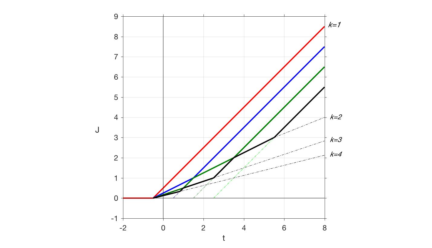
Figure 1: Leading (in red) and next three subleading (in blue, green, black) Regge trajectories of our model for $\alpha_{0}=\tfrac{1}{2}$. The sum of Regge poles turns into a branch point at $J=0$ below $t=-\tfrac{1}{2}$.

The structure becomes more and more complex as we go to even lower Regge poles. They always start asymptotically linear and parallel (as argued in [1]) with slope $\alpha^{\prime}$, but then they go through a series of breaks simulating a curved trajectory while remaining piecewise linear. This may turn out to be the only way to implement meromorphicity. Of course, we expect that, once higher orders in the large-$N$ expansion are included as in [8], the resulting trajectories will be smooth and curved and, correspondingly, resonances will acquire a finite width.

3.4 Tree-level unitarity

The most stringent constraint comes at this point from requiring tree-level unitarity which becomes nothing but positivity of the residues of each pole in $s$ for each definite $s$-channel angular momentum and isospin (these being the quantum numbers diagonalizing the unitarity constraint).

Note that the $I=2$ amplitude has no $s$-channel poles while the $I=0$ and $I=1$ amplitudes have only even and odd angular momenta. It thus turn out that a necessary and sufficient condition for tree-level unitarity is the one that can be imposed on $A(s,t)$ itself.

In the next section we will present the results we have been able to obtain so far on the unitarity issue.

4 Tree-level unitarity constraints

The issue of positivity of pole residues for all masses and spin is, to the best of our knowledge, an unsolved one even for the old LS amplitude. What is known in that case is that positivity is lost as soon as one moves away from a critical value $\alpha(0)=\tfrac{1}{2}$ of the intercept or from the dimensionality $D=4$ of space-time. Moving in the direction of a lower intercept and/or of a higher $D$ immediately turns a zero-norm state into a ghost. Although we have not found a rigorous proof, we have many numerical and analytic arguments in favor of positivity for all masses and spins in the $D=4,\alpha(0)=\tfrac{1}{2}$ case.

If we now move to our ansatz Eq.(3.2) for $D=4$, it is clear from what precedes that each individual amplitude $A_{k},\,k\neq 1$ will generically lead to negative residues because of their lower and lower intercept as $k$ is increased. It will be therefore quite non trivial to achieve positivity for $D=4$ and $\alpha(0)$ in the neighborhood of $\tfrac{1}{2}$.

4.1 Analytic results

Being able to prove analytically that, in a suitable region of parameter space, the positivity requirement is satisfied looks highly improbable. On the other hand one can certainly check positivity for the very first few levels and numerically for many of them (see below). The hope then is to be able to prove that if positivity holds up to a large mass level (and nay spin) it will keep holding all the way to infinitely large masses and spins. After all, while the first levels are deeply in the quantum regime, the high-mass and high-spin level should have a (semi)classical counterpart. And we do not expect unphysical properties in a classical string.

We have then looked at this regime by smoothing out the imaginary part of the amplitude (which gives nothing but its Regge limit)

$${\rm Im}A_{1}=\pi s^{\alpha_{0}}\left[\frac{s^{t}}{\Gamma(\alpha_{0}+t)}\right]\;,$$ (17)

and by replacing the Legendre projection by the well known passage from momentum transfer to impact parameter $b$ to be identified at large $s$ and $J$ with a continuous value for $2J/\sqrt{s}$.

It turns out that such a procedure can be easily implemented and that the needed Fourier-Bessel transform can be well approximated by a saddle point in the complex $t$ plane giving:

$$\log\left(\frac{1}{\pi}\Gamma(\alpha_{0})s^{-\alpha_{0}}{\rm Im}A_{1}(s,b)\right)=-\frac{b^{2}}{4W}+\frac{b^{2}Y}{16W^{2}}-\log\left[\frac{\Gamma(\alpha_{0}+\frac{b^{2}}{16W^{2}})}{\Gamma(\alpha_{0})}\right]\;,$$ (18)

where $W\equiv-W_{-1}(-\frac{J}{2s})$ is the lower branch of Lambert (product-log) function solving the equation:

$$\log W(x)-W(x)=\log(x)\,.$$ (19)

We have checked this expression against the numerical ones described below and found an amazingly good agreement over more than $20$ orders of magnitude (see Fig. 2). An advantage of this method is that it gives an explicitly positive result in its region of validity.

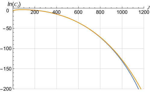
Figure 2: Log-plot of Legendre expansion coefficients $C_{J}$ by the saddle point (blue line) and by the algebraic method of Sec. A.1 up to $J=1200$.

One should then consider our superposition in Eq.(3.2)ñ of quantities like the one in (18) and check what conditions on the $c_{k}$ emerge from the positivity requirement. Using (13) the quantity to be considered is:

$${\rm Im}A=\pi\sum_{k}c_{k}\left(\frac{s}{k}\right)^{\alpha_{0}/k}\left[\frac{(\frac{s}{k})^{t/k}}{\Gamma(\frac{\alpha_{0}+t}{k})}\right]\;,$$ (20)

and therefore the needed generalization of (18) is:

$$\log\left(\frac{1}{\pi k}\Gamma(\frac{\alpha_{0}}{k})s^{-\frac{\alpha_{0}}{k}}{\rm Im}A_{k}(s,b)\right)=-\frac{kb^{2}}{4W_{k}}+\frac{b^{2}Y}{16W_{k}^{2}}-\log\left[\frac{\Gamma(\frac{\alpha_{0}}{k}+\frac{kb^{2}}{16W_{k}^{2}})}{\Gamma(\frac{\alpha_{0}}{k})}\right]\;,$$ (21)

where $W_{k}\equiv-W_{-1}(-\frac{kJ}{2s})$.

The results obtained by this method are shown in Fig. 2 and can be compared with the ones computed by the methods of next section. We plot the expansion coefficients $C_{J}$ in Legendre polynomials (not to be confused with the weights $c_{k}$ of Eq.(8)) in logarithmic scale. Agreement is even better with the numerical results obtained using Eq.(20).

Another analytic approach that we have tried, so far unsuccessfully, is of the induction type. If, above a certain $s=a+\bar{M}$, one could prove that positivity at $s=a+M$ implies positivity at $s=a+M+1$ one would be done. This looks like a hard but not impossible problem.

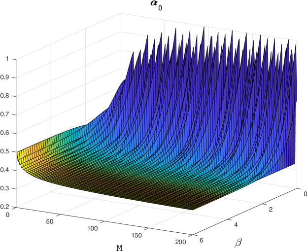
Figure 3: The “critical landscape”: $\alpha_{0}$ values above the surface give positive residues (here and in the following $\gamma=\beta+1$)

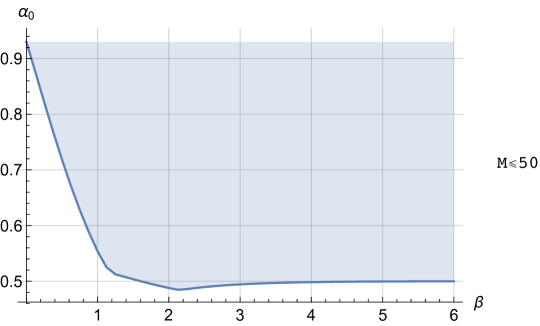
Figure 4: Same as the plot of Fig.3 projected on the ${\footnotesize(\beta,\alpha_{0})}$ plane. Shaded region corresponds to positive residues.

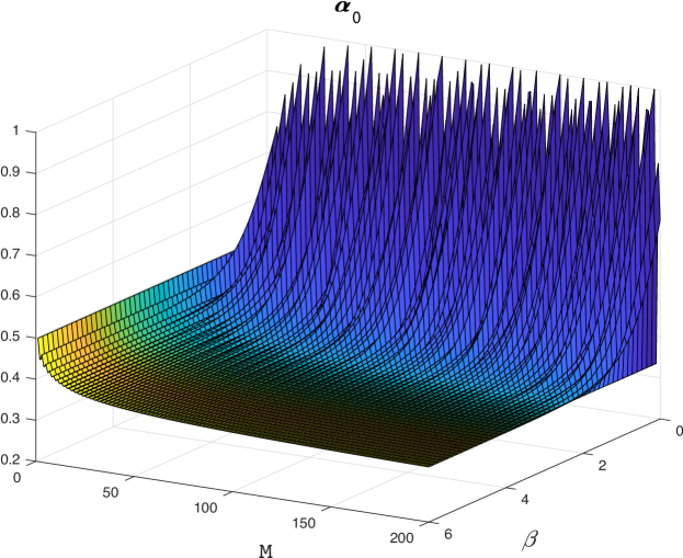
Figure 5: Same as Fig. 3 when the summation in Eq. (8) is restricted to odd divisors.

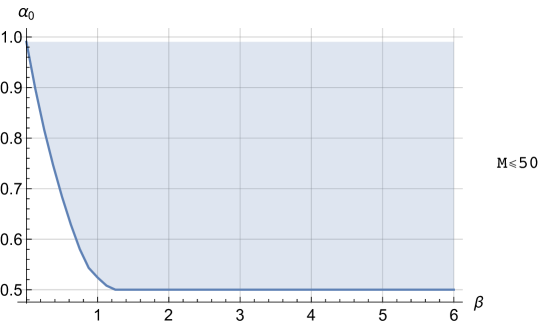
Figure 6: Same as the previous figure projected on the $(\beta,\alpha_{0})$ plane

4.2 Numerical results

The expansion of the function given in Eq. (8) (with the ansatz $c_{k}=k^{-\beta-1}\,(1+\ln(k))^{-\gamma}$) into a series of Legendre polynomials represents an apparently straightforward task involving a number of integrations of the kind $\int_{-1}^{1}\,f(z)\,P_{n}(z)\,dz$; still we have to face the problem that i) the number of integrals to be computed to explore the whole “critical landscape” is rather high (of the order of $\sim 10^{6}$) and ii) high accuracy is needed , since we are dealing with high order polynomials at the level of $O(10^{3})$ as required for the comparison with analytic data. Hence we have chosen an alternate strategy, that is presented in the Appendix. Here we limit ourselves to present the results of numerical computations as condensed in Fig. (3-6), where it is clear that there is an ample domain in $(\beta,\alpha_{0})$ plane where the unitarity constraint is satisfied. In Fig. 3 we present a bird’s view of the critical surface, while in Fig.4 we report the region in $(\beta,\alpha_{0})$ plane where the expansion coefficients are positive, which is equivalent to look at Fig. 3 in the direction of $M$-axis. Fig.s (5, 6) refer to the restriction of the sum in Eq. (8) to odd divisors of $M{\scriptstyle+}1$, whose motivation should be clear from the last part of the conclusions. Algorithmic details can be found in the Appendix.

5 Conclusions

Summarizing our results we should immediately remark that positivity of residues in the massless four point function is only a necessary condition for the unitarity of the model. Hence, not surprisingly there is ample room for satisfying such a (still non trivial) constraint. There is a-priori room for hidden degeneracy underlying poles of the 4-point amplitude and the no-ghost constraint demands positivity for each individual contribution to the residue at each given $s$, $J$ and $I$. To disentangle such a possible degeneracy and check for unitarity one has to consider also higher $n$-point amplitudes as it was done in the early days of string theory. At that point one should also impose positivity for elastic $2\rightarrow 2$ processes involving the massive sector of the theory, a point recently stressed by Arkani-Hamed [18]. Having amplitudes with two external excited states would also allow to construct QCD-string loops and check the expectation [19] that such loops, unlike those of the Nambu-Goto string, are UV-divergent. All this, however, is far beyond the scope of this paper.

To reconcile the universal exponential behavior of the amplitude at large positive $s$ and $t$ and it’s Regge behavior with the softer power (up to logs) behavior associated with AF, we need, effectively, a dominant Regge trajectory which is linear with slope 1 (in units of $\alpha^{\prime}$) at large positive $t$, but flattens out at negative $t$. Our model amplitude effectively achieves this by having an infinite sum of string amplitudes which differ by their slope (associated with the string tension), with the $k$th term in the sum having a slope of $1/k$. If we draw the leading linear trajectories associated with all these terms we see (Fig. 1) that the effective dominant (leading $J$ for fixed $t$) trajectory has a ”kink” at $t=-\alpha_{0}$. It coincides with the usual Regge trajectory for $t>-\alpha_{0}$ and with the large-$k$ zero-slope trajectory at $t<-\alpha_{0}$.

It is intriguing to compare this behavior with the one emerging in the holographic approach in Ref.[13] (for another holographically based approach to meson scattering amplitudes see also [20] and references therein). In the holographic approach of [13] there is only one string, however its slope depends (continuously) on the radial coordinate making the slope varying between 1 for small radial position (IR) to zero for large radial position (UV). The effective outcome structure for the dominant trajectory is again with the usual leading (IR) trajectory at large positive $t$ and a ”kink” at $t=-\alpha_{0}$ connecting to the constant slope (UV) trajectory in the $t<0$ region. Figure 1 in [13] clearly resembles our Fig.(1) and the mathematics which leads to the power (up to logs) law behavior for fixed angle scattering is quite similar. Of course in the holographic approach the slope varies continuously with the radial position and the computation of the amplitude involves an integration over the radial coordinate while we have just a discrete sum. Nevertheless the mathematical similarity leads in both cases to the softer power (up to logs) behavior in the AF region. If indeed the large-$N$ QCD will be proven to produce an amplitude as in our model, it would be tempting to try and understand/interpret the sum over $k$ as an indication for the existence of an holographic dimension. It may very well happen that at a certain level an interaction between the various strings corresponding to the different terms in our sum will have to be put in (without changing the qualitative behavior of the effective $\alpha(t)$ in our model) thus turning the discrete index $k$ into a continuous one corresponding to the holographic dimension.

To the extent that we take our model amplitude to be a first approximation to the large-$N$ QCD amplitude we would like to understand the origin of the sum over $k$ of string amplitudes with slopes $1/k$. Large -$N$ QCD is believed to be some sort of tree-level string theory. Moreover, lattice simulations [21, 22] and the expansion of the effective theory of long strings [23, 24] indicate that this string theory should be rather close to the Nambu-Goto string. The first term in our sum corresponds to such a string. What about the terms with $k>1$? One possible conjecture is that they correspond to folded strings [25] with the folding occurring precisely at the end-points of the open string (where the quark and anti-quark reside). Clearly, in order to account for the folded string to go from the quark to the antiquark, the number of folds must be even. The case of $2m$ folds corresponds to having a tension of $k=2m+1$ (or slope of $1/(2m+1)$ in $\alpha^{\prime}$ units) Hence, in order to account for such string configurations, the sum in (3.2) will be over odd integer $k$.

We have checked numerically that this still gives a unitary amplitude and it still satisfies all the demands that we have imposed in section 2. See Fig.s (5,6) where the allowed region has been computed with the technique of Sec. A.1; notice that the lower bound $\alpha_{0}\geq 1/2$ is due mainly to the $M=1$ data (as it is obvious from Fig.5)) for $\beta\geq\beta_{0}\approx 1.198...$, while for smaller values of $\beta$ there are more stringent bounds coming from higher values of $M$. For other values of $\gamma$ other than $\beta+1$ we checked that the picture is essentially the same, only the threshold $\beta_{0}$ is $\gamma$-dependent.

There is a-priori no reason we could think of why the folds should occur at exactly the endpoints. Actually they could occur anywhere. We wonder whether taking also such configurations into account will, effectively, make the tension continuous and therefore the slope to change continuously between one and zero. Having such a continuous slope may make the formal resemblance to the holographic approach of Ref.[13] even closer.

Appendix A Appendix

We present here the strategy we used to expand the function given in Eq. (8) into a series of Legendre polynomials; to be specific we assume the coefficients in Eq. (8) to be $c_{k}=k^{-\beta-1}\,(1+\ln(k))^{-\gamma}$ and typically, unless differently specified, $\gamma=\beta+1$, as anticipated in Sec. 3.3.1. The problem of Legendre expansion received much attention in the last decades, and an account can be found in Ref.s [14, 15]. Fast techniques have also been implemented in popular packages like Chebfun working under Matlab. We had to recourse to a different strategy because we need essentially unlimited arithmetic accuracy to go beyond $M\approx O(100)$, and this is not possible with Chebfun. The algorithms we are going to present can be implemented either in Mathematica, where one works with rationals and the results are exact, or adopting a multiple precision software like advanpix. We note here that an entirely different approach could be adopted making recourse to a classical result of Schoenberg [16]: a function $f(z),({\scriptstyle-}1<z<1)$ is “of positive type on $S^{2}$”, if for any set of unit vectors $\{v_{j},j=1...n\}$ the matrix $f(v_{i}\cdot v_{j})$ is positive definite. Such a function of positive type has an expansion in Legendre polynomials with non-negative coefficients (and converse). We are exploring this property as an alternative to the direct computation of the Legendre expansion by implementing a kind of MonteCarlo on the space of $n$-tuples of unit vectors. Results will be reported elsewhere.

We used both approaches, “algebraic” and “spectral”, to derive the unitarity region in $(\beta,\alpha_{0})$. The first method has the additional advantage that the calculations can be performed leaving $\alpha_{0}$ and $\beta$ symbolic. Since the calculation can be done in unlimited precision we consider the numerical evidence as founded on solid ground, and it is nice to have a perfect match with the analytic saddle point technique. Let us note that the spectral method can be applied also to a non-polynomial $f(z)$ and this allowed to compare the numerical result with that obtained by a saddle point technique in Sec.4.1 using Eq.(17).

A.1 The algebraic algorithm

We have to expand a polynomial already given in factorized form, hence we can simply apply the recursion relation of Legendre polynomials

$$z\,P_{n}(z)=\frac{n+1}{2n+1}\,P_{n+1}(z)+\frac{n}{2n+1}\,P_{n-1}$$ (22)

step by step. The problem is reduced to a simple algebraic calculation, very easily implemented in a symbolic language like Mathematica. The code starts with the vector representing $P_{0}(z)$, $\phi_{0}=(1,0,0,\ldots,0,0)$ of length $M{\scriptstyle+}2$ and one can apply the various factors of the polynomial of Eq.(8) by substituting the variable $z$ with the matrix

$$Z=\begin{pmatrix}0&\frac{1}{3}&0&0&0&0&\ldots\\ 1&0&\frac{2}{5}&0&0&0&\ldots\\ 0&\frac{2}{3}&0&\frac{3}{7}&0&0&\ldots\\ 0&0&\frac{3}{5}&0&\frac{4}{9}&0&\ldots\\ \vdots&&&\ddots&&\ddots&\end{pmatrix}$$ (23)

as obtained by the recursion relation (22) expressed in terms of the vector’s components. The final result is obtained by summing over all divisors of $M{\scriptstyle+}1$ (or over odd divisors for the case discussed in the conclusion section); we get the critical value for $a$ by a customary bisection method. This method is essentially exact, since step by step all components are rational numbers which can be treated with no truncation errors and the bisection method can be pushed to any desired accuracy. The algebraic approach allowed us to explore the positivity region for values of $M$ well above $10^{3}$. The only logical limitation is due to the fact that we can compute the coefficients only up to some finite value of $M$: how can we exclude that for some bigger value negative coefficients could possibly show up for the same values of the other parameters? We can’t, but the overall picture and the asymptotic (analytic) formulae give us the confidence that this is not going to happen.

A.2 The spectral method

Another approach, allowing to get some additional insight into the problem, can be applied to any function, not just to polynomials. If we restrict the expansion to a maximum order $n=M{\scriptstyle+}1$ than we are working with a finite dimensional truncation of the matrix $Z$. Its spectral properties are well-known thanks to a result of Golub and Welsch about Gaussian quadrature [17]: its eigenvalues are given by the zeroes $z_{j}$ of $P_{M{\scriptstyle+}2}(z)$ and its $j\mbox{-}$th eigenvector is given by

$${\mathcal{P}}^{(j)}=\left\{\sqrt{w_{j}}\,P_{n}\left(z_{j}\right)\,\mid\,{\smallish n=0\ldots M{\scriptstyle+}1}\right\}$$

where $\{w_{j}\}$ are the Gaussian weights for the $(M{\scriptstyle+}2){\scriptstyle-}$dimensional quadrature rule. The zeros are all distinct and belong to the interval $(-1,1)$; the leading eigenvalue (i.e. the one closest to 1, by convention assigned to $j=1$) corresponds to an eigenvector with all positive components. This is clear from the properties of zeroes of orthogonal polynomials, but it is also an immediate consequence of Perron-Frobenius theorem about positive matrices (and our matrix is actually a stochastic matrix). The expansion in Legendre polynomials is thus converted into an expansion in eigenvectors of the matrix $Z^{(M{\scriptstyle+}2)}$, and for any function $f(z)$ we simply get (dropping for simplicity the index $M{\scriptstyle+}2$)

$$f(Z)_{n,m}\,=\,\sum_{j}\,f(z_{j})\,{\mathcal{P}}^{(j)}_{n}\,{\mathcal{P}}^{(j)}_{m}$$

The expansion coefficients we want to compute are obtained by applying this matrix to the vector $\phi_{0}$ hence we simply get $C_{n}=f(Z)_{n,0}\equiv\sum_{j}\,w_{j}\,f(z_{j})\,P_{n}(z_{j})$, which is nothing but Gauss’ quadrature formula which is exact for polynomials of degree $\leq 2M{\scriptstyle+}1$. The expansion coefficients we have to compute are obtained by identifying $f(z)$ with the r.h.s. of Eq.(8) or Eq.(20), hence the spectral approach is exact when applied to Eq. (8) while it is affected by an error, which can in principle be estimated, in the other case. For $K=1$ the function is sharply peaked near $z=1$ so that the leading eigenvector $j=1$ is dominant. The situation is different for $k>1$ and the final result comes from a delicate balance of all these contributions and it depends on $M$ and on the value of $\alpha_{0}$. So we expect that for $\alpha_{0}$ sufficiently large the first eigenvector with all positive components will be dominant, but only the explicit calculation can identify the critical value of $\alpha_{0}$ above which we get unitarity (see Figs. 4 and 6: allowed values for $\alpha_{0}$ lie within the shaded region).

References

- [1] S. Caron-Huot, Z. Komargodski, A. Sever and A. Zhiboedov, arXiv:1607.04253 [hep-th].
- [2] G. Veneziano, Nuovo Cim. A 57, 190 (1968).
- [3] D. J. Gross and P. F. Mende, Phys. Lett. B 197, 129 (1987).
- [4] O.Andreev and W.Siegel, Phys. Rev. D 71, 086001 (2005), [hep-th/0410131].
- [5] C. Lovelace, Phys. Lett. 28B, 264 (1968).
- [6] J. A. Shapiro, Phys. Rev. 179, 1345 (1969).
- [7] G. ’t Hooft, Nucl. Phys. B 72, 461 (1974).
- [8] G. Veneziano, Nucl. Phys. B 117, 519 (1976).
- [9] S. J. Brodsky and G. R. Farrar, Phys. Rev. Lett. 31, 1153 (1973).
- [10] G. P. Lepage and S. J. Brodsky, Phys. Rev. D 22, 2157 (1980).
- [11] G. Veneziano, Phys. Rept. 9, 199 (1974).
- [12] R. Dolen, D. Horn and C. Schmid, Phys. Rev. 166, 1768 (1968).
- [13] R. C. Brower, J. Polchinski, M. J. Strassler and C. I. Tan, JHEP 0712, 005 (2007), [hep-th/0603115].
- [14] B. Alpert and V. Rokhlin, SIAM J. Sci. and Stat. Comput., 12(1), (1991) 158–179
- [15] N. Hale and A. Townsend, SIAM J. Sci. Comp. 36 (2014) A148-A167.
- [16] I.J. Schoenberg, Duke Math. J., 9, No.1, 1942.
- [17] G.H.Golub and J.H.Welsch, Math. Comput. 23 (1969) 221-230.
- [18] N. Arkani-Hamed, talk given at the S-Matrix bootstrap workshop, EPFL Lausanne, Jan. 2017.
- [19] M. Bochicchio, arXiv:1606.04546 [hep-th].
- [20] A. Armoni and E. Ireson, arXiv:1611.00342 [hep-th].
- [21] A. Athenodorou, B. Bringoltz and M. Teper, JHEP 1102, 030 (2011), [arXiv:1007.4720 [hep-lat]].
- [22] B. B. Brandt and M. Meineri, Int. J. Mod. Phys. A 31, no. 22, 1643001 (2016), [arXiv:1603.06969 [hep-th]].
- [23] O. Aharony and N. Klinghoffer, JHEP 1012, 058 (2010), [arXiv:1008.2648 [hep-th]].
- [24] O. Aharony and Z. Komargodski, JHEP 1305, 118 (2013), [arXiv:1302.6257 [hep-th]].
- [25] O. Ganor, J. Sonnenschein and S. Yankielowicz, Nucl. Phys. B 434, 139 (1995), [hep-th/9407114].