Physics without physics

Abstract

David Finkelstein was very fond of the new information-theoretic paradigm of physics advocated by John Archibald Wheeler and Richard Feynman. Only recently, however, the paradigm has concretely shown its full power, with the derivation of quantum theory chiribella2011informational ; QTfromprinciples and of free quantum field theory PhysRevA.90.062106 ; bisio2013dirac ; Bisio2015244 ; Bisio2016 from informational principles. The paradigm has opened for the first time the possibility of avoiding physical primitives in the axioms of the physical theory, allowing a re-foundation of the whole physics over logically solid grounds. In addition to such methodological value, the new information-theoretic derivation of quantum field theory is particularly interesting for establishing a theoretical framework for quantum gravity, with the idea of obtaining gravity itself as emergent from the quantum information processing, as also suggested by the role played by information in the holographic principle susskind1995world ; bousso2002holographic .

In this paper I review how free quantum field theory is derived without using mechanical primitives, including space-time, special relativity, Hamiltonians, and quantization rules. The theory is simply provided by the simplest quantum algorithm encompassing a countable set of quantum systems whose network of interactions satisfies the three following simple principles: homogeneity, locality, and isotropy.

The inherent discrete nature of the informational derivation leads to an extension of quantum field theory in terms of a quantum cellular automata and quantum walks. A simple heuristic argument sets the scale to the Planck one, and the currently observed regime where discreteness is not visible is the so-called “relativistic regime” of small wavevectors, which holds for all energies ever tested (and even much larger), where the usual free quantum field theory is perfectly recovered.

In the present quantum discrete theory Einstein relativity principle can be restated without using space-time in terms of invariance of the eigenvalue equation of the automaton/walk under change of representations. Distortions of the Poincaré group emerge at the Planck scale, whereas special relativity is perfectly recovered in the relativistic regime. Discreteness, on the other hand, has some plus compared to the continuum theory: 1) it contains it as a special regime; 2) it leads to some additional features with GR flavor: the existence of an upper bound for the particle mass (with physical interpretation as the Planck mass), and a global De Sitter invariance; 3) it provides its own physical standards for space, time, and mass within a purely mathematical adimensional context.

The paper ends with the future perspectives of this project, and with an appendix containing biographic notes about my friendship with David Finkelstein, to whom this paper is dedicated.

Beware the Lorelei of Mathematics. Her song is beautiful.

David Finkelstein

1 Introduction

The logical clash between General Relativity (GR) and Quantum Field Theory (QFT) is the main open problem in physics. The two theories represent our best theoretical frameworks, and work astonishingly well within the physical domain for which they have been designed. However, their logical clash requires us to admit that they cannot be both correct. One could argue that there must exist a common theoretical substratum from which both theories emerge as approximate effective theories in their pertaining domains–though we know very little about GR in the domain of particle physics.

What we should keep and what we should reject of the two theories? Our experience has thought us that of QFT we should definitely keep the Quantum Theory (QT) of abstract systems, namely the theory of the von Neumann book john1955mathematical stripped of its “mechanical” part, i. e. the Schrödinger equation and the quantization rules. This leaves us with the description of generic systems in terms of Hilbert spaces, unitary transformations, and observables. In other words, this is what nowadays is also called Quantum Information, a research field indeed very interdisciplinary in physics.

There are two main reasons for keeping QT as valid. First, it has been never falsified in any experiment in the whole physical domain–independently of the scale and the kind of system. This has lead the vast majority of physicists to believe that everything must behave according to QT. The second and more relevant reason is that QT, differently from any other chapter of physics, is well axiomatized, with purely mathematical axioms containing no physical primitive. So, in a sense, QT is as valid as a piece of pure mathematics. This must be contrasted with the mechanical part of the theory, with the bad axiomatic of the so-called “quantization rules”, which are extrapolated and generalized starting from the heuristic argument of the Ehrenfest theorem, which in turn is based on the superseded theory of classical mechanics, and with the additional problem of the ordering of canonical noncommuting observables. No wonder then that the quantization procedure doesn’t work well for gravity!

To what we said above we should add that today we know that the QT of von Neumann can be derived from six information-theoretical principles chiribella2011informational ; QTfromprinciples , whose epistemological value is not easy to give up. On the contrary, it is the mechanical part of QFT that rises the main inconsistencies, e .g. the Malament theorem halvorson2002no , which makes any reasonable notion of particle untenable kuhlmann2015real .

The logical conclusion is that what we need is a field theory that is quantum ab initio. But how to avoid quantization rules? The idea is simply to consider a countable set of quantum systems in interaction, and to make the easiest assumptions on the topology of their interactions. These are: locality, homogeneity, and isotropy. Notice that we are not using any mechanics, nor relativity, and not even space and time. And what we get? We get: Weyl, Dirac PhysRevA.90.062106 , and Maxwell Bisio2016 . Namely: we get free quantum field theory!

The new general methodology suggested to the above experience is then the following: 1) no physical primitives in the axioms; 2) physics only as interpretation of the mathematics (based on experience, previous theories, and heuristics). In this way the logical coherence of the theory is mathematically guaranteed. In this review we will see how the proposed methodology can be actually carried out, and how the informational paradigm has the potential of solving the conflict between QFT and GR in the case of special relativity, with the latter emergent merely from quantum systems in interaction: Fermionic quantum bits at the very tiny Planck scale. In synthesis the program is an algorithmization of theoretical physics, aimed to derive the whole physics from quantum algorithms with finite complexity, upon connecting the algebraic properties of the algorithm with the dynamical features of the physical theory, preparing a logically coherent framework for a theory of quantum gravity.

Section 2 is devoted to the derivation from principles of the quantum-walk theory. More precisely, from the requirements of homogeneity and locality of the interactions of countably many quantum systems one gets a theory of quantum cellular automata on the Cayley graph of a group $G$. Then, upon restricting to the simple case of evolution linear in the discrete fields, the quantum automaton becomes what is called in the literature quantum walk. We further restrict to the case with physical interpretation in an Euclidean space, resorting to considering only Abelian $G$.

In Section 3 the quantum walks with minimal field dimension that follow from the principles of Sect. 2 are reported. These represent the Planck-scale version of the Weyl, Dirac, and Maxwell quantum field dynamics, which are recovered in the relativistic regime of small wavevectors. Indeed, the quantum-walk theory, being purely mathematical–and so adimensional–nevertheless contains its own physical LTM standards written in the intrinsic discreteness and non-linearities of the theory. A simple heuristic argument based on the notion of mini black-hole (from a matching of GR-QFT) leads to the Planck scale. It follows that the relativistic regime contains the whole physics observed up to now, including the most energetic events from cosmic rays.

In addition to the exact dynamics in terms of quantum walks, a simple analytical method is also available in terms of a dispersive Schrödinger equation, suitable to the Planck-scale physics for narrow-band wave-packets. As a result of the unitarity constraint for the evolution, the particle mass turns out to be upper bounded (by the Planck mass), and has domain in a circle, corresponding to having also the proper-time (which is conjugated to the mass) as discrete. Effects due to discreteness that are in principle visible are also analyzed, in particular a dispersive behavior of the vacuum, that can be detected by deep-space ultra-high energy cosmic rays.

Section 4 is devoted to how special relativity is recovered from the quantum-walk discrete theory, without using space-time and kinematics. It is shown that the transformation group is a non-linear version of the Poincaré group, which recovers the usual linear group in the relativistic limit of small wavevectors. For nonvanishing masses generally also the mass gets involved in the transformations, and the De Sitter group $SO(1,4)$ is obtained.

The paper ends with a brief section on the future perspectives of the theory, and with an Appendix about my first encounter with David Finkelstein.

Most of results reported in the present review have been originally published in Refs. PhysRevA.90.062106 ; bisio2013dirac ; Bisio2015244 ; Bisio2016 ; reviewderiv ; reviewanaly ; mauro2012quantum ; lrntz3d ; FOPDP16 ; d2015virtually coauthored with members of the QUit group in Pavia.

2 Derivation from principles of the quantum-walk theory

If you are receptive and humble, mathematics will lead you by the hand.

Paul Dirac

The derivation from principles of quantum field theory starts from considering the unitary evolution $\mathcal{A}$ of a countable set $G$ of quantum systems, with the requirements of homogeneity, locality, and isotropy of their mutual interactions. These will be precisely defined and analyzed in following dedicated subsections. All the three requirements are dictated from the general principle of minimizing the algorithmic complexity of the physical law. The physical law itself is described by a finite quantum algorithm, and homogeneity and isotropy assess the universality of the law.

The quantum system labeled by $g\in G$ can be either associated to an Hilbert space ${\cal{K}}_{g}$, or to a set of generators of a C^∗-algebra

$$\psi_{g}\equiv\{\psi_{g}^{\nu}\},\qquad g\in G,\quad\nu\in[s_{g}]:=\{1,2,\ldots,s_{g}\},\;s_{g}<\infty.$$ (1)

The evolution occurs in discrete identical steps

$$\mathcal{A}\psi_{g}=U\psi_{g}U^{\dagger},\quad U\text{unitary,}$$ (2)

describing the interactions among systems. When the unitary evolution is also local, namely $\mathcal{A}\psi_{g}$ is spanned by a finite subset $S_{g}\subset G$, then $\mathcal{A}$ is called Quantum Cellular Automaton. We restrict to evolution linear in the generators, namely

$$\mathcal{A}\psi_{g}=U\psi_{g}U^{\dagger}=\sum_{g^{\prime}}A_{g,g^{\prime}}\psi_{g^{\prime}},$$ (3)

where $A_{g,g^{\prime}}$ is an $s_{g}\times s_{g^{\prime}}$ complex matrix called transition matrix. Here in all respects the quantum cellular automaton is described by a unitary evolution on a (generally infinite) Hilbert space ${\cal{H}}=\bigoplus_{g\in G}{\cal{H}}_{g}$, with ${\cal{H}}_{g}=\mathsf{Span}\{\psi_{g}^{\nu}\}_{\nu\in[s_{g}]}$. In this case the quantum cellular automaton is called Quantum Walk. Here the system simply corresponds to a finite-dimensional block component of the Hilbert space, regardless the Bosonic/Fermionic nature of the field. In the derivation of free quantum field theory from principles, the quantum walk corresponds to the evolution on the single-particle sector of the Fock space, whereas for the interacting theory a generally nonlinear quantum cellular automaton is needed. Simple generalization to Fock-space sectors with fixed number of particles are also possible.

2.1 The quantum system: qubit, Fermion or Boson?

At the level of quantum walks, corresponding to the Fock space description of cellular quantum automata (leading to free QFT in the nonrelativistic limit), it does not make any difference which kind of quantum system is evolving. Indeed one can symmetrize or anti-symmetrize products of wavefunctions, as it is done in usual quantum mechanics, or else just take products with no symmetrization. Things become different when the vacuum is considered, and particles are created and annihilated by operating with algebra generators on the vacuum state, as in the interacting theory. Therefore, as far as we are concerned with free QFT, which kind of quantum system should be used is a problem that can be safely postponed.

However, there are still motivations for adopting a kind of quantum system instead of another. For example, a reason for discarding qubits as algebra generators is that there is no easy way of expressing the operator $U$ making the evolution in Eq. (3) linear, whereas, when $\psi_{g}$ is Bosonic or Fermionic this is always possible choosing $U$ exponential of bilinear forms in the fields. On the other hand, a reason to chose Fermions instead of Bosons is the requirement that the amount of information in a finite number of cells be finite, namely one has finite information density in space. The relation between Fermionic modes and finite-dimensional quantum systems, say qubits has been studied in the literature, and the two theories have been proven to be computationally equivalent Bravyi2002210 . However, the quantum theory of qubits and the quantum theory of Fermions differ in the notion of what are local transformations IJMP14 ; EPL14 , with local Fermionic operations mapped into nonlocal qubit transformations and vice versa.

In conclusion, the derivation from informational principles of the fundamental particle statistics still remains an open problem. One could promote the finite information density to the level of a principle, or motivate the Fermionic statistics from other principles of the same nature of those in Ref. chiribella2011informational (see e. g. Refs. IJMP14 ; EPL14 ), or derive the Fermionic statistics from properties of the vacuum (e. g. having a localized non-entangled vacuum in order to avoid the problem of particle localization), and then recover the Bosonic statistics as a very good approximation, with the Bosonic mode corresponding to a special entangled state of pairs of Fermionic modes Bisio2016 , as it will be reviewed in Subsect. 3.9. This hierarchical construction will also guarantee the validity of the spin-statistic connection in QFT.

2.2 Quantum Walks on Cayley graphs

The linear Eq. (3) endows the set $G$ with a directed graph structure $\Gamma(G,E)$, with vertex set $G$ and edge set $E=\{(g,g^{\prime})|A_{g,g^{\prime}}\neq 0\}$ directed from $g$ to $g^{\prime}$ (see Fig. 1). In the following we will denote by $S_{g}:=\{A_{g,g^{\prime}}\neq 0\}$ the set of non-null transition matrices with first index $g$, and by $N_{g}:=\{g^{\prime}\in G|A_{g,g^{\prime}}\neq 0\}$ the neighborhood of $g$.

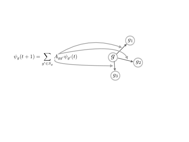
Figure 1: The linear Eq. (3) endows the set $G$ with a directed graph structure. We build a directed graph with an arrow from $g$ to $g^{\prime}$ wherever the two are connected by a nonnull matrix $A_{gg^{\prime}}$ in Eq. (3).

2.2.1 The homogeneity principle

The assumption of homogeneity is the requirement that every two vertices are indistinguishable, namely for every $g,g^{\prime}\in G$ there exists a permutation $\pi$ of $G$ such that $\pi(g)=g^{\prime}$ which commute with any discrimination procedure consisting of a preparation of local modes followed by a general joint measurement. In Ref. FOPDP16 it is shown that this is equivalent to the following set of conditions

$\forall g\in G$ one has:

1. $s_{g}=s$;

2. there exists a bijection $N_{g}\leftrightarrow N$ with a fixed set $N$;

3. $S_{g}$ contains the same $s\times s$ transition matrices, namely $S_{g}=S:=\{A_{h_{1}}\}_{i=1}^{|N|}$;

4. $A_{g,g^{\prime}}=A_{h_{i}}\in S$ $\Rightarrow$ $A_{g^{\prime},g}=A_{h_{j}}\in S$;

Condition H2 states that $\Gamma(G,E)$ is a regular graph—i. e. each vertex has the same degree. Condition H3 makes $\Gamma(G,E)$ a colored directed graph, with the arrow directed from $g$ to $g^{\prime}$ for $A_{g,g^{\prime}}=A_{h}\in S$ and the color associated to $h$. Condition H3 introduces the following formal action of symbols $h_{i}\in S$ on the elements $g\in G$ as

$$A_{gg^{\prime}}=A_{h_{i}}\Rightarrow gh_{i}=g^{\prime}.$$ (4)

Clearly such action is closed for composition. From condition H4 one has that

$$A_{g^{\prime}g}=A_{h_{j}}\Rightarrow g^{\prime}h_{j}=g,$$ (5)

and composing the two actions we see that $gh_{i}h_{j}=g$, and we can write the label $h_{j}$ as $h_{j}=:h_{i}^{-1}$. We thus can build the free group $F$ of words made with the alphabet $S$. Each word corresponds to a path over $\Gamma(G,E)$, and the words $w\in F$ such that $gw=g$ correspond to closed paths (also called loops). Notice that by construction, one has $A_{\pi(g)\pi(f)}=A_{gf}=A_{h_{i}}$, which implies that $\pi(g)h_{i}=\pi(f)=\pi(gh_{i})$, from which one can prove that $f^{\prime}w=\pi(f)w=\pi(fw)=\pi(f)=f^{\prime}$ (see FOPDP16 ). Thus we have the following

1. If a path $w\in F$ is closed starting from $f\in G$, then it is closed also starting from any other $g\in G$.

The subset $R\subset F$ of words $w$ such that $gw=g$ is obviously a group. Moreover $R$ is a normal subgroup of $G$, since $gwrw^{-1}=(gw)rw^{-1}=(gw)w^{-1}=g$, namely $wrw^{-1}\in R$ $\forall w\in F,\forall r\in R$. Obviously the equivalence classes are just elements of $G$, which means that $G=F/R$ is a group. Pick up any element of $G$ as the identity $e\in G$. It is clear that the elements of the quotient group $F/R$ are in one-to-one correspondence with the elements of $G$, since for every $g\in G$ there is only one class in $F/R$ whose elements lead from $e$ to $g$ (write $g=ew$ for every $w\in F$, $w$ representing a path leading from $e$ to $g$). The graph $\Gamma(G,E)$ is thus what is called in the literature the Cayley graph of the group $G$ (see the definition in the following). The Cayley graph is in correspondence with a presentation of the group $G$. This is usually given by arbitrarily dividing the set as $S=S_{+}\cup S_{-}$ with $S_{-}:=S_{+}^{-1}$, and by considering a set $W$ of generators for the free group of loops $R$. The group $G$ is then given with the presentation $G=\langle S_{+}|W\rangle$, in terms of the set of its generators $S_{+}$ (which along with their inverses $S_{-}$ generate the group by composition), and in terms of the set of its relators $W$ containing group words that are equal to the identity, with the goal of using these words in $W$ to establish if any two words of elements of $G$ correspond to te same group element. The relators can also be regarded as a set of generators for $R$.

The definition of Cayley graph is then the following.

Cayley graph of $G$.

Given a group $G$ and a set $S_{+}$ of generators of the group, the Cayley graph $\Gamma(G,S_{+})$ is defined as the colored directed graph with vertex set $G$, edge set $\{(g,gh);g\in G,h\in S_{+}\}$ with the edge directed from $g$ to $gh$ with color assigned by $h$ (when $h=h^{-1}$ we conventionally draw an undirected edge).

Notice that a Cayley graph in addition to being a regular graph, it is also vertex-transitive—i. e. all sites are equivalent, in the sense that the graph automorphism group acts transitively upon its vertices. The Cayley graph is also called arc-transitive when its group of automorphisms acts transitively not only on its vertices but also on its directed edges.

2.2.2 The locality principle

Locality corresponds to require that the evolution is completely determined by a rule involving a finite number of systems. This means having each system interacting with a finite number of systems (i. e. $|N|<\infty$ in H2), and having the set of loops generating $F$ as finite and containing only finite loops. This corresponds to the fact that the group $G$ is finitely presented, namely both $S_{+}$ and $W$ are finite in $G=\langle S_{+}|W\rangle$.

The quantum walk then corresponds to a unitary operator over the Hilbert space ${\cal{H}}=\ell^{2}(G)\otimes\mathbb{C}^{s}$ of the form

$$A=\sum_{h\in S}T_{h}\otimes A_{h},$$ (6)

where $T$ is the right-regular representation of $G$ on $\ell^{2}(G)$, $T_{g}|g^{\prime}\rangle=|g^{\prime}g^{-1}\rangle$.

2.2.3 The isotropy principle

The requirement of isotropy corresponds to the statement that all directions on $\Gamma(G,S_{+})$ are equivalent. Technically the principle affirms that there exists a choice of $S_{+}$, a group $L$ of graph automorphisms on $\Gamma(G,S_{+})$ that is transitive over $S_{+}$ and with faithful unitary (generally projective) representation $U$ over $\mathbb{C}^{s}$, such that the following covariance condition holds

$$A=\sum_{h\in S}T_{h}\otimes A_{h}=\sum_{h\in S}T_{l(h)}\otimes U_{l}A_{h}U^{\dagger}_{l},\quad\forall l\in L.$$ (7)

As a consequence of the linear independence of the generators $T_{h}$ of the right regular representation of $G$ one has that the above condition (7) implies

$$A_{l(h^{\pm 1})}=U_{l}A_{h^{\pm 1}}U_{l}^{\dagger}.$$ (8)

Eq. (8) implies that the principle of isotropy requires the Cayley graph $\Gamma(G,S_{+})$ to be arc-transitive (see Subsect. 2.2.1).

We remind that the split $S=S_{+}\cup S_{-}$ is non unique (and in addition one may add to $S$ the identity element $e$ corresponding to zero-length loops on each element corresponding to self-interactions). Therefore, generally the quantum walk on the Cayley graph $\Gamma(G,S_{+})$ satisfies isotropy only for some choices of the set $S_{+}$. It happens that for the known cases satisfying all principles along with the restriction to quasi isometric embeddability of $G$ in Euclidean space (see Subsect. 2.3) such choice is unique.

2.2.4 The unitarity principle

The requirement that the evolution be unitary translates into the following set of equations bilinear in the transition matrices as unknown

$$\sum_{h\in S}A^{\dagger}_{h}A_{h}=\sum_{h\in S}A_{h}A^{\dagger}_{h}=I_{s},\qquad\sum_{\shortstack{$\scriptstyle h,h^{\prime}\in S$\\ $\scriptstyle h^{-1}h^{\prime}=h^{\prime\prime}$}}A^{\dagger}_{h}A_{h^{\prime}}=\sum_{\shortstack{$\scriptstyle h,h^{\prime}\in S$\\ $\scriptstyle h^{\prime}h^{-1}=h^{\prime\prime}$}}A_{h^{\prime}}A^{\dagger}_{h}=0.$$ (9)

Notice that the structure of equations already satisfy the homogeneity and locality principles. The solution of the systems of equations (9) is generally a difficult problem.

2.3 Restriction to Euclidean emergent space

How a discrete quantum algorithm on a graph can give rise to a continuum quantum field theory on space-time? We remind that the flow of the quantum state occurs on a Cayley graph and the evolution occurs in discrete steps. Therefore the Cayley graph must play the role of a discretized space, whereas the steps play the role of a discretized time, namely the quantum automaton/walk has an inherent Cartesian-product structure of space-time, corresponding to a particular chosen observer. We will then need a procedure for recovering the emergent space-time and a re-interpretation of the notion of inertial frame and of boost in the discrete, in order to recover Poincaré covariance and the Minkowski structure. The route for such procedure is opened by geometric group theory, a field in pure mathematics initiated by Mikhail Gromov at the beginning of the nineteen. The founding idea is the notion of quasi-isometric embedding, which allows us to compare spaces with very different metrics, as for the cases of continuum and discrete. Clearly an isometric embedding of a space with a discrete metric (as for the word metric of the Cayley graph) within a space with a continuum metric (as for a Riemaniann manifold) is not possible. However, what Gromov realized to be geometrically relevant is the feature that the discrepancy between the two different metrics is uniformly bounded over the spaces. More precisely, one introduces the following notion of quasi-isometry.

Quasi-isometry.

Given two metric spaces $(M_{1},d_{1})$ and $(M_{2},d_{2})$, with metric $d_{1}$ and $d_{2}$, respectively, a map $f:(M_{1},d_{1})\rightarrow(M_{2},d_{2})$ is a quasi-isometry if there exist constants $A\geq 1$, $B,C\geq 0$, such that $\forall g_{1},g_{2}\in M_{1}$ one has

$$\frac{1}{A}d_{1}(g_{1},g_{2})-B\leq d_{2}(f(g_{1}),f(g_{2}))\leq Ad_{1}(g_{1},g_{2})+B,$$ (10)

and $\forall m\in M_{2}$ there exists $g\in M_{1}$ such that

$$d_{2}(f(g),m)\leq C.$$ (11)

The condition in Eq. (11) is also called quasi-onto.

It is easy to see that quasi-isometry is an equivalence relation. It can also be proved that the quasi-isometric class is an invariant of the group, i. e. it does not depend on the presentation, i. e. on the Cayley graph. Moreover, it is particularly interesting for us that for finitely generated groups, the quasi-isometry class always contains a smooth Riemaniann manifold harpe . Therefore, for a given Cayley graph there always exists a Riemaniann manifold in which it can be quasi-isometrically embedded, which is unique modulo quasi-isometries, and which depends only on the group $G$ of the Cayley graph. Two examples are graphically represented in Fig. 2.

2.3.1 Geometric group theory

With the idea of quasi-isometric embedding, geometric group theory connects geometric properties of the embedding Riemaniann spaces with algebraic properties of the groups, opening the route to a geometrization of group theory, including the generally hard problem of establishing properties of a group that is given by presentation only.

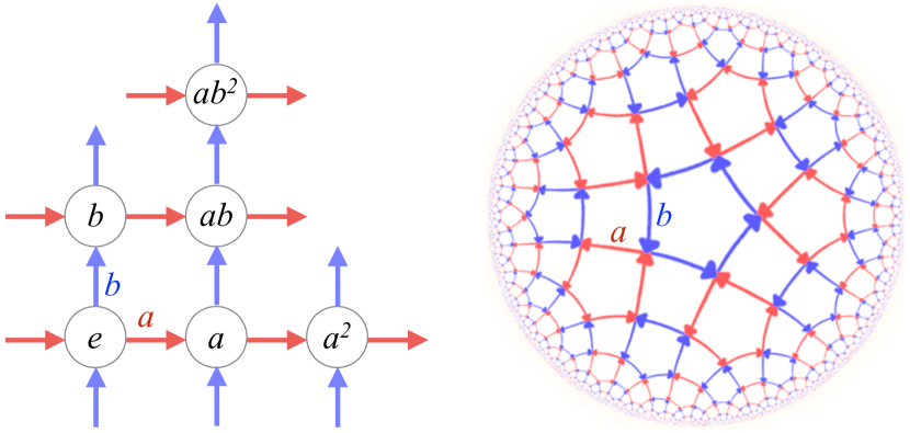
Figure 2: From Ref. FOPDP16 . (Colors online). Given a group $G$ and a set $S_{+}$ of generators, the Cayley graph $\Gamma(G,S_{+})$ is defined as the colored directed graph having set of nodes $G$, set of edges $\{(g,gh);g\in G,h\in S_{+}\}$, and a color assigned to each generator $h\in S_{+}$. Left figure: the Cayley graph of the Abelian group $\mathbb{Z}^{2}$ with presentation $\mathbb{Z}^{2}=\langle a,b|aba^{-1}b^{-1}\rangle$, where a and b are two commuting generators. Right figure: the Cayley graph of the non-Abelian group $G=\langle a,b|a^{5},b^{5},(ab)^{2}\rangle$. The Abelian-group graph is embedded into the Euclidean space $\mathbb{R}^{2}$, the non-Abelian $G$ into the Hyperbolic space $\mathbb{H}_{2}$ with negative curvature.

The possible groups $G$ that are selected from our principles are infinitely many, and we need to restrict this set to start the search for solutions of the unitarity conditions (2.3) under the isotropy constraint. Since we are interested in a theory involving infinitely many systems (we take the world as infinite!), we will consider infinite groups only. This means that when we consider an Abelian group, we always take it as free, namely its only relators are those establishing the Abelianity of the group. This is the case of $G=\mathbb{Z}^{d}$, with $d\geq 1$.

A paradigmatic result harpe of geometric group theory is that an infinite group $G$ is quasi-isometric to an Euclidean space $\mathbb{R}^{d}$ if and only if $G$ is virtually-Abelian, namely it has an Abelian subgroup $G^{\prime}\subset G$ isomorphic to $\mathbb{Z}^{d}$ of finite index (namely with a finite number of cosets). Another result is that a group has polinomial growth iff it is virtually-nihilpotent, and if it has exponential growth then it not virtually-nihilpotent, and in particular non Abelian, and is quasi-isometrically embeddable in a manifold with negative curvature.

In the following we will restrict to groups that are quasi-isometrically embeddable in Euclidean spaces. As we will see soon, such restriction will indeed lead us to free quantum field theory in Euclidean space. It would be very interesting to address also the case of curved spaces, to get hints about quantum field theory in curved space. Unfortunately, the case of negative curvature corresponds to groups, as the Fuchsian group in Fig. 2, whose unitary representations (that we need here) are still unknown Farb ; Drutu ; Tessera . The virtually-nihilpotent case also would be interesting, since it corresponds to a Riemaniann manifold with variable curvature Tessera , however, a Cayley graph that can satisfy the isotropy constraint could not be found yet unpubDEP .

I close this section with some comments about the remarkable closeness in spirit between the present program and the geometric group theory program. The main general goal of geometric group theory is the geometrization of group theory, which is achieved studying finitely-generated groups $G$ as symmetry groups of metric spaces $X$, with the aim of establish connections between the algebraic structure of $G$ with the geometric properties of $X$ Kapovich-notes . In a specular way the present program is an algorithmization of theoretical physics, with the general goal of deriving QFT (and ultimately the whole physics) from quantum algorithms with finite complexity, upon connecting the algebraic properties of the algorithm with the dynamical features of the physical theory. This will allow a coherent unified axiomatization of physics without physical primitives, preparing a logically coherent framework for a theory of quantum gravity.

3 Quantum Walks on Abelian groups and free QFT as their relativistic regime

As seen in Subsect. 2.3, from the huge and yet mathematically unexplored set of possibilities for the group $G$ of the quantum walk, we restrict to the case of $G$ virtually-Abelian, which corresponds to $G$ quasi-isometrically embeddable in an Euclidean space. As we will see in the present section, the free QFT that will be derived from such choice exactly corresponds to the known QFT in Euclidean space.

Since we are interested in the physics occurring in $\mathbb{R}^{3}$, we need to classify all possible Cayley graphs of $G$ having $\mathbb{Z}^{3}$ as subgroup with finite index, and then select all graphs that allow the quantum walk to satisfy the conditions of isotropy and unitarity. We can proceed by considering increasingly large dimension $s>0$ (defined in H1), which ultimately corresponds to the dimension of the field–e .g. a scalar field for $s=1$, a spinor field for $s=2$, etc.

3.1 Induced representation, and reduction from virtually Abelian to Abelian quantum walks

An easy way to classify all quantum walks on Cayley graphs with virtually Abelian groups is provided by a theorem in Ref. d2015virtually , which establishes the following

A quantum walk on the Cayley graph of a virtually Abelian group $G$ with Abelian subgroup $H\subset G$ of finite index $i_{H}$ and dimension $s$ is also a quantum walk on the Cayley graph of $H$ with dimension $s^{\prime}=si_{H}$.

This is just the induced-representation theorem mackey1951induced ; mackey1952induced ; mackey1953induced in group theory, here applied to quantum walks. The multiple dimension $s^{\prime}=si_{h}$ corresponds to tiling the Cayley graph of $G$ with a tile made with a particular choice of the cosets of $H$. The new set of transition matrices of the new walk for $H$ can be straightforwardly evaluated in terms of those for $G$ (generally self interactions within the same tile can occur, corresponding to zero-length loops in the Cayley graph). In Fig. 3 two examples of such tiling procedure are given.

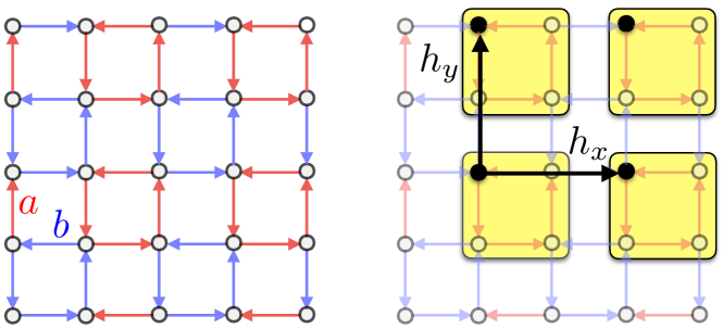
Figure 3: From Ref. d2015virtually . (Colors online). Two examples of reduction of a quantum walk on the Cayley graph of a virtually Abelian group $G$ to that of a quantum walk on the Cayley graph of an Abelian subgroup $H\subset G$ with finite index $i_{H}$. The graphs on the left of the figures are the Cayley graph of $G$ (it is easy to see that both groups are non Abelian). The graphs on the right represents a choice of the Cayley graph of the subgroup $H=\mathbb{Z}^{2}$, with the tiling corresponding to the induced representation (the elements of $H$ are the black bullets). Top figures: $G=\langle a,b\ |\ a^{4},b^{4},{\left(ab\right)}^{2}\rangle$. The index is $i_{H}=4$. The subgroup generators are $h_{x}=a^{-1}b$ and $h_{y}=ba^{-1}$. The tiling is defined by the coset representatives $e,a,a^{2},a^{3}$. Bottom figures: $G=\langle a,b\ |\ a^{2}b^{-2}\rangle$. The index is $i_{H}=2$. The subgroup generators are $h_{1}=ba$ and $h_{2}=a^{2}$ (or $h_{1}=ba$ and $h_{3}=ab^{-1}$), with the tiling the cosets representatives $e,a$.

The induced-representation method guarantees that scanning all possible virtually Abelian quantum walks for increasing $s$ is equivalent to scan all possible Abelian quantum walks, since e. g. the set of Abelian walks of dimension $s=nm$ will contain all virtually Abelian walks with $s=n$ and index $m$, etc. We therefore resort to consider only Abelian groups.

3.2 Isotropy and orthogonal embedding in $\mathbb{R}^{3}$

We will also assume that the representation of the isotropy group $L$ in (7) induced by the embedding in $\mathbb{R}^{3}$ is orthogonal, which implies that the graph-neighborhood is embedded in a sphere $S^{2}\subset\mathbb{R}^{3}$ (we want homogeneity and isotropy to hold locally also in the embedding space $\mathbb{R}^{3}$). We are then left with the classification of the Cayley graphs of $\mathbb{Z}^{3}$ satisfying the isotropic embedding in $\mathbb{R}^{3}$: these are just the Bravais lattices.

3.3 Quantum Walks with Abelian $G$

When $G$ is Abelian we can greatly simplify the study of the quantum walk by using the wave-vector representation, based on the fact that the irreducible representations of $G$ are one-dimensional. The interesting case is for $d=3$, but what follows holds for any dimension $d$. We will label the group elements by vectors $\mathbf{g}\in\mathbb{Z}^{d}$, and use the additive notation for the group composition, whereas the right-regular representation of $\mathbb{Z}^{d}$ on $\ell_{2}(\mathbb{Z}^{d})$ will be written as $T_{\mathbf{h}}|\mathbf{g}\rangle=|\mathbf{g}-\mathbf{h}\rangle$. This can be diagonalized by Fourier transform, corresponding to write the operator $A$ in block-form in terms of the following direct-integral

$$A=\int_{B}\operatorname{d}^{3}\!\mathbf{k}\,|{\mathbf{k}}\rangle\langle{\mathbf{k}}|\otimes A_{\mathbf{k}},\qquad A_{\mathbf{k}}:=\sum_{\mathbf{h}\in S}e^{-i\mathbf{k}\cdot\mathbf{h}}A_{\mathbf{h}},\quad|\mathbf{k}\rangle:=\frac{1}{\sqrt{|B|}}\sum_{\mathbf{g}\in G}e^{-i\mathbf{k}\cdot\mathbf{g}}|\mathbf{g}\rangle.$$ (12)

where $B$ is the Brillouin zone, and $|\mathbf{k}\rangle$ is a plane wave. Notice that the quantum walk is unitary if and only if $A_{\mathbf{k}}$ is unitary for every $\mathbf{k}\in B$.

3.4 Dispersion relation

The spectrum $\{e^{-i\omega^{(i)}_{\mathbf{k}}}\}$ of the operator $A_{\mathbf{k}}$ is usually given in terms of the so-called dispersion relations $\omega^{(i)}_{\mathbf{k}}$ versus $\mathbf{k}$. As in usual wave-mechanics, the speed of the wave-front of a plane wave is given by the phase-velocity $\omega^{(i)}_{\mathbf{k}}/|\mathbf{k}|$, whereas the speed of a narrow-band packet peaked around the value wave-vector $\mathbf{k}_{0}$ is given by the group velocity $\nabla_{\mathbf{k}}\omega^{(i)}_{\mathbf{k}}$ evaluated at $\mathbf{k}_{0}$.

3.5 The relativistic regime

As we will see in Sect. 3.8.3 an heuristic argument will lead us to set the scale of discreteness of the quantum walk (and similarly the quantum cellular automaton for the interacting theory) at the Planck scale. The domain $|\mathbf{k}|\ll 1$ then corresponds to wave-vectors much smaller than the Planck vector, which is much higher than any ever observed wave-vector. Such regime includes that of usual particle physics, and is called relativistic regime. To be precise, the regime is defined by a set of wavepackets that are peacked around $\mathbf{k}=0$ with r.m.s. value much smaller than the Planck wave-vector, which we will refer shortly to as narrow-band wave-packets.

I want to emphasize here that we have never used any mechanical concept in our derivation of the quantum walk, including the notion of Hamiltonian: the dynamics is given in term of a single unitary operator $A$. A notion of effective Hamiltonian could be considered as the logarithm of $A$, which would correspond to an Hamiltonian providing the same unitary evolution, and which would even interpolate it between contiguous steps. For this reason we will call such an operator interpolating Hamiltonian. In the Fourier direct-integral representation of the operator, the interpolating Hamiltonian will be given by the identity $e^{-iH(\mathbf{k})}:=A_{\mathbf{k}}$. It is easy to see that the relativistic limit $H_{0}(\mathbf{k})$ of $H(\mathbf{k})$, corresponding to consider narrow-band wave-packets centered at $\mathbf{k}=0$, is achieved by expanding it at the first order in $|\mathbf{k}|$, i. e. $H(\mathbf{k})=H_{0}(\mathbf{k})+\mathcal{O}(|\mathbf{k}|^{2})$. The interpolated continuum-time evolution in the relativistic regime will be then given by the first-order differential equation in the Schrödinger form

$$i\partial_{t}\psi(\mathbf{k},t)=H_{0}(\mathbf{k})\psi(\mathbf{k},t).$$ (13)

Rigorous quantitative approaches to judge the closeness between free QFT and the relativistic regime of the quantum walk have been provided in Ref. Bisio2015244 in terms of channel discrimination probability, and in Ref.  PhysRevA.90.062106 in terms of fidelity between the two evolutions. Numerical values will be provided at the end of Subsect. 3.8.

3.6 Schrödinger equation for the ultra-relativistic regime

In the ultra-relativistic regime of wave-vectors comparable to the Planck vector, an obvious option is that of evaluating the evolution by a numerical evaluation of the exact quantum walk. However, even in such regime we still have an analytical method available for evaluating the evolution of some common physical states. Indeed, for narrow-band wave packets centered around any value $\mathbf{k}_{0}$ one can write a dispersive Schrödinger equation by expanding the interpolating Hamiltonian $H(\mathbf{k})$ around $\mathbf{k}_{0}$ at the second order, thus obtaining

$$i\partial_{t}\tilde{\psi}(\mathbf{x},t)=\pm[\mathbf{v}\cdot\mathbf{\nabla}+\tfrac{1}{2}\mathbf{D}\cdot\mathbf{\nabla}\mathbf{\nabla}]\tilde{\psi}(\mathbf{x},t),$$ (14)

where $\tilde{\psi}(\mathbf{x},t)$ is the Fourier transform of $\tilde{\psi}(\mathbf{k},t):=e^{-i\mathbf{k}_{0}\cdot\mathbf{x}+i\omega_{0}t}\psi(\mathbf{k},t)$, $\mathbf{v}=\left(\mathbf{\nabla}_{\mathbf{k}}\omega\right)(\mathbf{k}_{0})$ is the drift vector, and $\mathbf{D}=\left(\mathbf{\nabla}_{\mathbf{k}}\mathbf{\nabla}_{\mathbf{k}}\omega\right)(\mathbf{k}_{0})$ is the diffusion tensor. This equation approximates very well the evolution, even in the Planck regime and for large numbers of steps, depending on the bandwith (see an example in Fig. 4 from Ref. Bisio2015244 ).

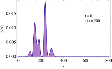
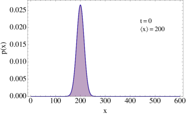
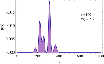
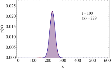
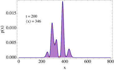
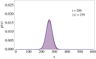
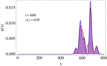
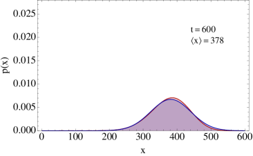
Figure 4: From Ref. Bisio2015244 . (Colors online). Test of the quality of the approximation of the Schrödinger equation (14) at for different time $t$ of the Dirac quantum walk with mass $m=0.6$ in one space dimension of Ref.Bisio2015244 . Comparison of the probability distribution (in red) and the solution of the Schrödinger equation (in blue). Right figures: the state is a superposition of Hermite functions multiplied by the Gaussian peaked around momentum $k_{0}=3\pi/10$, for drift and diffusion coefficients $v=0.73$ and $D=0.31$, respectively. The mean value moves at the group velocity given by the drift coefficient $v$. The approximation remains accurate even for position spread $\hat{\sigma}=20$ Planck lengths. Left figures: The same four times comparison for the quantum walk with $m=0.4$, and an initial Gaussian state peaked around the momentum $k_{0}=0.1$. In this case the drift velocity and the diffusion coefficient are respectively $v=0.22$ and $D=2.30$.

3.7 Recovering the Weyl equation

In Subsect. 3.2 we were left with the classification of the Cayley graphs of $\mathbb{Z}^{3}$ satisfying the isotropic embedding in $\mathbb{R}^{3}$, which are just the Bravais lattices. For dimension $s=1$ it is easy to show that the only solution of the unitarity constraints gives the trivial quantum walk $A=I$. We then consider $s=2$. Now, the only inequivalent isotropic Cayley graphs are the primitive cubic (PC) lattice, the body centered cubic (BCC), and the rhombohedral. However only in the BCC case, whose presentation of $\mathbb{Z}^{3}$ involves four vectors $S_{+}=\{\mathbf{h}_{1},\mathbf{h}_{2},\mathbf{h}_{3},\mathbf{h}_{4}\}$ with relator $\mathbf{h}_{1}+\mathbf{h}_{2}+\mathbf{h}_{3}+\mathbf{h}_{4}=0$, one finds solutions satisfying all the assumptions of Section 2. The isotropy group is given by the group $L$ of binary rotations around the coordinate axes, with the unitary projective representation on $\mathbb{C}^{2}$ given by $\{I,i\sigma_{x},i\sigma_{y},i\sigma_{z}\}$. The group $L$ is transitive on the four BCC generators of $S_{+}$. There are only four solutions (modulo unitary conjugation) that can be divided in two pairs $A^{\pm}$ and $B^{\pm}$. The two pairs of solutions are connected by transposition in the canonical basis, i. e. $A_{\mathbf{k}}^{\pm}=(B_{\mathbf{k}}^{\pm})^{T}$. The solutions $B_{\mathbf{k}}^{\pm}$ can be also obtained from the solution $A_{\mathbf{k}}^{\pm}$ by shifting the wave-vector $\mathbf{k}$ inside the Brillouin zone to the vectors PhysRevA.90.062106

$$\mathbf{k_{1}}=\frac{\pi}{2}(1,1,1),\quad\mathbf{k_{2}}=-\frac{\pi}{2}(1,1,1),\quad\mathbf{k_{3}}=-\frac{\pi}{2}(1,0,0).$$ (15)

The $A_{\mathbf{k}}^{\pm}$ solutions in the wave-vector representation are

$$A^{\pm}_{\mathbf{k}}=Iu^{\pm}_{\mathbf{k}}-i\bm{\sigma}^{\pm}\cdot\tilde{\mathbf{n}}^{\pm}_{\mathbf{k}}$$ (16)

with

$${\tilde{\mathbf{n}}}^{\pm}_{\mathbf{k}}:=\begin{pmatrix}s_{x}c_{y}c_{z}\mp c_{x}s_{y}s_{z}\\ c_{x}s_{y}c_{z}\pm s_{x}c_{y}s_{z}\\ c_{x}c_{y}s_{z}\mp s_{x}s_{y}c_{z}\end{pmatrix},\quad u^{\pm}_{\mathbf{k}}:=c_{x}c_{y}c_{z}\pm s_{x}s_{y}s_{z},\\$$ (17)

where $c_{i}:=\cos(k_{i}/\sqrt{3})$, $s_{i}:=\sin(k_{i}/\sqrt{3})$, and $\bm{\sigma}^{+}=\bm{\sigma}$, $\bm{\sigma}^{-}=\bm{\sigma}^{T}$. The spectrum of $A^{\pm}_{\mathbf{k}}$ is $\{e^{-i\omega^{\pm}}_{\mathbf{k}}\}$, with dispersion relation given by

$$\omega^{\pm}_{\mathbf{k}}=\arccos(c_{x}c_{y}c_{z}\mp s_{x}s_{y}s_{z}).$$ (18)

It is easy to get the relativistic limit of the quantum walk using the procedure in Subsect. 3.5. This simply corresponds to substituting $c_{i}=1$ and $s_{i}=k_{i}/\sqrt{3}$ in Eq. (17), thus obtaining

$$i\partial_{t}\psi(\mathbf{k},t)=\frac{1}{\sqrt{3}}\bm{\sigma}^{\pm}\cdot\mathbf{k}\,\psi(\mathbf{k},t).$$ (19)

Eqs. (19) are the two Weyl equations for the left and the right chiralities. For $G=\mathbb{Z}^{d}$ with $d=1,2$ one obtains the Weyl equations in dimension $d=1,2$, respectively PhysRevA.90.062106 . All the three quantum walks have the same form in Eq. (16), namely

$$A_{\mathbf{k}}=u_{\mathbf{k}}I-i\bm{\sigma}\cdot\tilde{\mathbf{n}}_{\mathbf{k}},$$ (20)

with dispersion relation

$$\omega_{\mathbf{k}}=\arccos{u_{\mathbf{k}}},$$ (21)

and with the analytic expression of $u_{k}$ and $\mathbf{n}_{k}$ depending on $d$ and on the chirality (see Ref. PhysRevA.90.062106 ). Since the quantum walks in Eq. (17) or (20) have the Weyl equations as relativistic limit, we will also call them Weyl quantum walks.

The interpolating Hamiltonian is $H(\mathbf{k})=\bm{\sigma}\cdot\mathbf{n}_{\mathbf{k}}$, with $\mathbf{n}_{\mathbf{k}}:=(\omega_{\mathbf{k}}/\sin\omega_{\mathbf{k}})\tilde{\mathbf{n}}_{\mathbf{k}}$ playing the role of an helicity vector, and with relativistic-limit being given by $H_{0}(\mathbf{k})=\tfrac{1}{\sqrt{d}}\bm{\sigma}\cdot\mathbf{k}$, which coincides with the usual Weyl Hamiltonian in $d$ dimensions upon interpreting the wave-vector $\mathbf{k}$ as the particle momentum.

We conclude the present subsection by emphasizing that one additional advantages of the discrete framework is that the Feynman path-integral is well defined, and it is also exactly calculated analytically in some cases. Indeed, in Refs. path1d and path2d the discrete Feynman propagator for the Weyl quantum walk has been analytically evaluated with a closed form for dimensions $d=1$ and $d=2$, and the case of dimension $d=3$ will be published soon path3d .

3.8 Recovering the Dirac equation

From subsection 3.7 we know that all quantum walks derivable from our principles for $s=2$ give the Weyl equation in the relativistic limit. We now need to increase the dimension $s$ of the field beyond $s=2$. However, the problem of solving the unitarity equations (9) becomes increasingly difficult, since the unknown are matrices of increasingly larger dimension $s\geq 3$ (we remind that the equations are bilinear non homogeneus in the unknown transition matrices, and a canonical procedure for the solution is unknown). What we can do for the moment is to provide only some particular solutions using algebraic techniques. Two ways of obtaining solutions for $s=4$ is to start from solutions in dimension $s=2$ and built the direct-sum and tensor product of two copies of the quantum walk in such a way that the obtained quantum walk for dimension $s=4$ still satisfies the principles. We will see that the quantum walks that we obtain in the relativistic limit give the Dirac equation when using the direct sum, whereas they give the Maxwell equation (plus a static scalar field) when we use the tensor product.

When building a quantum walk in $2\times 2$ block form, all four blocks must be quantum walks themselves. The requirement of locality of the coupling leads to off-diagonal blocks that do not depend on $\mathbf{k}$. A detailed analysis of the restrictions due to the unitarity conditions (9) shows that, modulo unitary change of representation independent on $\mathbf{k}$, we can take the off-diagonal matrix elements as proportional to the identity, whereas the diagonal blocks are just given by the chosen quantum walk and its adjoint, respectively. We then need to weight the diagonal blocks with a constant $n$ and the off-diagonal identities with a constant $m$, and unitarity requires having $|n|^{2}+|m|^{2}=1$. Then, starting from the walk $A_{\mathbf{k}}$ that leads us to the Weyl equations for all dimension $d=1,2,3$, the walk, modulo unitary equivalence, can be recast in the formPhysRevA.90.062106

$$D_{\mathbf{k}}:=\begin{pmatrix}nA_{\mathbf{k}}&im\\ im&nA_{\mathbf{k}}^{\dagger}\end{pmatrix},\qquad n^{2}+m^{2}=1,\;n\in\mathbb{R}^{+},m\in\mathbb{R}.$$ (22)

Also the sign of $m$ can be changed by a unitary equivalence (a “charge-conjugation”), however, we keep $m$ with changing sign for reasons that will explained in Subsect. 3.8.2. The walk (22) with $s=4$ can be conveniently expressed in terms of gamma matrices in the spinorial representation as follows

$$D_{\mathbf{k}}:=nIu_{\mathbf{k}}-in\gamma^{0}\bm{\gamma}\cdot\tilde{\mathbf{n}}_{\mathbf{k}}+im\gamma^{0},$$ (23)

where the functions $u_{\mathbf{k}}$ and $\tilde{\mathbf{n}}_{\mathbf{k}}$ depend on the choice of $A_{\mathbf{k}}$ in Eq. (22), i. e. on $d=1,2,3$. The dispersion relation of the quantum walk (23) is simply given by

$$\omega_{\mathbf{k}}=\arccos[\sqrt{1-m^{2}}u_{\mathbf{k}}].$$ (24)

We will see now that the quantum walks in Eq. (22) in the small wave-vector limit and for $m\ll 1$ all give the usual Dirac equation in the respective dimension $d$, with $m$ corresponding to the particle rest mass, whereas $n$ works as the inverse of a refraction index of vacuum. In fact, the interpolating Hamiltonian $H(\mathbf{k})$ is given by

$$H(\mathbf{k})=\frac{\omega_{\mathbf{k}}}{\sin\omega_{\mathbf{k}}}(n\gamma^{0}\bm{\gamma}\cdot\tilde{\mathbf{n}}_{\mathbf{k}}-m\gamma^{0}),$$ (25)

with relativistic limit given by

$$H_{0}(\mathbf{k})=\frac{n}{\sqrt{d}}\gamma^{0}\bm{\gamma}\cdot\mathbf{k}+m\gamma^{0},$$ (26)

and to the order $\mathcal{O}(m^{2})$ we get the Dirac Hamiltonian

$$H_{0}(\mathbf{k})=\frac{1}{\sqrt{d}}\gamma^{0}\bm{\gamma}\cdot\mathbf{k}+m\gamma^{0}.$$ (27)

One has the Dirac Hamiltonian, with the wave-vector $\mathbf{k}$ interpreted as momentum and the parameter $m$ interpreted as the rest mass of the particle. In the relativistic limit (26) the parameter $n$ plays the role of the inverse of a refraction index of vacuum. In principle this can produce measurable effects from bursts of high-energy particles of different masses at the boundary of the visible universe, and would be complementary to the dispersive nature of vacuum (see subsections 3.8.3 and 3.9.2).

In the following we will also call the quantum walk in Eq. (22) Dirac quantum walk.

In Ref. path1d the discrete Feynman propagator for the Dirac quantum walk has been analytically evaluated with a closed formal for dimension $d=1$, generalizing the solution of Ref. kauffman1996discrete for fixed mass value.

3.8.1 Discriminability between quantum walk and quantum field dynamics

In Subsect. 3.5 we mentioned that rigorous quantitative approaches to judge the closeness between the two dynamics have been provided in Ref. Bisio2015244 , and in Ref. PhysRevA.90.062106 in terms of fidelity between the two unitary evolutions. For the Dirac quantum walk for a proton mass one has fidelity close to unit for $N\simeq m^{-3}=2.2*10^{57}$, corresponding to $t=1.2*10^{14}\text{s}=3.7*10^{6}$ years. The approximation is still good in the ultra-relativistic case $k\gg m$, e. g. for $k=10^{-8}$ (as for an ultra-high energy cosmic ray), where it holds for $N\simeq k^{-2}=10^{16}$ steps, corresponding to $5*10^{-28}$ s. However, one should notice that practically the discriminability in terms of fidelity corresponds to having unbounded technology, and such a short time very likely corresponds to unfeasible experiments. On the other hand, for a ultra-high energy proton with wave packet width of 100 fm the time required for discriminating the wave-packet of the quantum walk from that of QFT is comparable with the age of the universe.

3.8.2 Mass and proper-time

The unitarity requirement in Eq. (22) restrict the rest mass to belong to the interval

$$m\in[-1,1].$$ (28)

At the extreme points $\pm 1$ of the interval the corresponding dynamics $D_{\mathbf{k}}=\pm i\gamma^{0}$ are identical (they differ for an irrelevant global phase factor). This means that the domain of the mass has actually the topology of a circle, namely

$$m\in S^{1}.$$ (29)

From the classical relativistic Hamiltonian greenberger1970theory

$$H=\vec{p}\cdot\vec{q}+c^{2}m\tau-L,$$ (30)

with $\vec{p}$ and $\vec{q}$ canonically conjugated position and momentum and $L$ the Lagrangian, we see that the proper time $\tau$ is canonically conjugated to the rest mass $m$. This suggests that the Fourier conjugate of the rest mass in the quantum walk can be interpreted as the proper time of a particle evolution, and being the mass a variable in $S^{1}$, we conclude that the proper time is discrete, in accordance with the discreteness of the dynamical evolution of the quantum walk. This result constitutes a non trivial logical coherence check of the present quantum walk theory.

3.8.3 Physical dimensions and scales for mass and discreteness

We want to emphasize that in the above derivation everything is adimensional by construction. Dimensions can be recovered by using as measurement standards for space, time, and mass the discreteness scale for space $a_{*}$ and time $t_{*}$ ($a_{*}$ is half of the BCC cell side, $t_{*}$ the time-length of the unit step), along with the maximum value of the mass $m_{*}$ (corresponding to $|m|=1$ in Eq. (22)). From the relativistic limit, the comparison with the usual dimensional Dirac equation leads to the identities

$$c=a_{*}/t_{*},\quad\hbar=m_{*}a_{*}c,$$ (31)

which leave only one unknown among the three variables $a_{*},t_{*}$ and $m_{*}$. At the maximum value of the mass $|m|=1$ in Eq. (22) we get a flat dispersion relation, corresponding to no flow of information: this is naturally interpreted as a mini black-hole, i. e. a particle with Schwarzild radius equal to the localization length, i. e. the Compton wavelength. This leads to an heuristic interpretation of $m_{*}$ as the Planck mass, and from the two identities in Eq. (31) we get the Planck scale for discreteness. Notice that the value of $m_{*}$ can be in principle obtained from the dispersion of vacuum as $m_{*}\simeq\frac{1}{\sqrt{3}}\frac{\hbar k}{c(k)-c(0)}$ for small $k$, which can be in principle measured by the Fermi telescope from detection of ultra high energy bursts coming from deep space.

3.9 Recovering Maxwell fields

In Sections 3.7 and 3.8 we showed how the dynamics of free quantum fields can be derived starting from a countable set of quantum systems with a network of interactions satisfying the principles of locality, homogeneity, and isotropy. Within the present finitistic local-algorithmic perspective one also considers each system as carrying a finite amount of information, thus restricting the quantum field to be Fermionic (see also Subsect. 2.1). However, one may wonder how the physics of the free electromagnetic field can be recovered in such a way and, generally, how Bosonic fields are recovered from Fermionic ones. In this section we answers to these questions. The basic idea behind is that the photon emerges as an entangled pair of Fermions evolving according to the Weyl quantum walk of Section 3.7. Then one shows that in a suitable regime both the free Maxwell equation in 3d and the Bosonic commutation relations are recovered. Since in this subsection we are actually considering operator quantum fields, we will use more properly the quantum automaton nomenclature instead of the quantum walk one.

Consider two Fermionic fields $\psi(\mathbf{k})$ and $\varphi(\mathbf{k})$ in the wave-vector representation, with respective evolutions given by

$${\psi}(\mathbf{k},t+1)=W_{\mathbf{k}}{\psi}(\mathbf{k},t).\quad{\varphi}(\mathbf{k},t+1)=W_{\mathbf{k}}^{*}{\varphi}(\mathbf{k},t).$$ (32)

The matrix $W_{\mathbf{k}}$ can be any of the Weyl quantum walks for $d=3$ in Eq. (16), (the whole derivation is independent on this choice), whereas $W_{\mathbf{k}}^{*}=\sigma_{y}W_{\mathbf{k}}\sigma_{y}$ denotes the complex conjugate matrix. We introduce the bilinear operators

$$G^{i}(\mathbf{k},t):=\varphi^{T}(\tfrac{\mathbf{k}}{2},t)\sigma^{i}\psi(\tfrac{\mathbf{k}}{2},t)=\varphi^{T}(\mathbf{k},0)(W_{\tfrac{\mathbf{k}}{2}}^{\dagger}\sigma^{i}W_{\tfrac{\mathbf{k}}{2}})\psi(\tfrac{\mathbf{k}}{2},0)$$ (33)

by which we construct the vector field

$$\mathbf{G}(\mathbf{k},t):=(G^{1}(\mathbf{k},t),G^{2}(\mathbf{k},t),G^{3}(\mathbf{k},t))^{T}$$ (34)

and the transverse field

$$\mathbf{G}_{T}(\mathbf{k},t):=\mathbf{G}(\mathbf{k},t)-\left(\frac{\mathbf{n}_{\frac{\mathbf{k}}{2}}}{|\mathbf{n}_{\frac{\mathbf{k}}{2}}|}\cdot{\mathbf{G}}(\mathbf{k},t)\right)\frac{\mathbf{n}_{\frac{\mathbf{k}}{2}}}{|\mathbf{n}_{\frac{\mathbf{k}}{2}}|},$$ (35)

with $\mathbf{n}_{\mathbf{k}}:=(\omega_{\mathbf{k}}/\sin\omega_{\mathbf{k}})\tilde{\mathbf{n}}_{\mathbf{k}}$ and $\tilde{\mathbf{n}}_{\mathbf{k}}$ given in Eq. (17). By construction the field $\mathbf{G}_{T}(\mathbf{k},t)$ satisfies the following relations

$$\mathbf{n}_{\frac{\mathbf{k}}{2}}\cdot\mathbf{G}_{T}(\mathbf{k},t) =0,$$ (36)

$$\mathbf{G}_{T}(\mathbf{k},t) =\operatorname{Exp}(-i2\mathbf{n}_{\tfrac{\mathbf{k}}{2}}\cdot\mathbf{J}t)\mathbf{G}_{T}(\mathbf{k},0),$$ (37)

where we used the identity

$$\exp(-\tfrac{i}{2}\mathbf{v}\cdot\bm{\sigma})\bm{\sigma}\exp(\tfrac{i}{2}\mathbf{v}\cdot\bm{\sigma})=\operatorname{Exp}(-i\mathbf{v}\cdot\mathbf{J})\bm{\sigma},$$ (38)

the matrix $\operatorname{Exp}(-i\mathbf{v}\cdot\mathbf{J})$ acting on $\bm{\sigma}$ regarded as a vector, and $\mathbf{J}=(J_{x},J_{y},J_{z})$ representing the infinitesimal generators of $\mathbb{SU}(2)$ in the spin 1 representation. Taking the time derivative of Eq. (37) we obtain

$$\partial_{t}\mathbf{G}_{T}(\mathbf{k},t)=2\mathbf{n}_{\tfrac{\mathbf{k}}{2}}\times\mathbf{G}_{T}(\mathbf{k},t).$$ (39)

If $\mathbf{E}_{G}$ and $\mathbf{B}_{G}$ are two Hermitian operators defined by the relation

$$\mathbf{E}_{G}:=|{\mathbf{n}}_{\tfrac{\mathbf{k}}{2}}|(\mathbf{G}_{T}+\mathbf{G}_{T}^{\dagger}),\quad\mathbf{B}_{G}:=i|{\mathbf{n}}_{\tfrac{\mathbf{k}}{2}}|(\mathbf{G}_{T}^{\dagger}-\mathbf{G}_{T}),$$ (40)

then Eq. (36) and Eq. (39) can be rewritten as

$$\partial_{t}\mathbf{E}_{G}=i2\mathbf{n}_{\tfrac{\mathbf{k}}{2}}\times\mathbf{B}_{T}(\mathbf{k},t) \partial_{t}\mathbf{B}_{G}=-i2\mathbf{n}_{\tfrac{\mathbf{k}}{2}}\times\mathbf{E}_{T}(\mathbf{k},t)$$

$$2\mathbf{n}_{\tfrac{\mathbf{k}}{2}}\cdot\mathbf{E}_{G}=0 2\mathbf{n}_{\tfrac{\mathbf{k}}{2}}\cdot\mathbf{B}_{G}=0.$$ (41)

Eqs. (41) have the form of distorted Maxwell equations, with the wave-vector $\mathbf{k}$ substituted by $2\mathbf{n}_{\tfrac{\mathbf{k}}{2}}$, and in the relativistic limit $|\mathbf{k}|\ll 1$ one has $2\mathbf{n}_{\tfrac{\mathbf{k}}{2}}\sim\mathbf{k}$ and the usual free electrodynamics is recovered.

3.9.1 Photons made of pairs of Fermions

Since in the Weyl equation the field is Fermionic, the field defined in Eqs. (35) and (40) generally does not satisfy the correct Bosonic commutation relations. The solution to this problem is to replace the operator $\mathbf{G}$ defined in Eq. (35) with the operator $\mathbf{F}$ defined as

$$\mathbf{F}(\mathbf{k}):=\int\frac{d\mathbf{q}}{(2\pi)^{3}}f_{\mathbf{k}}(\mathbf{q})\varphi\left(\tfrac{\mathbf{k}}{2}-\mathbf{q}\right)\,\bm{\sigma}\,\psi\left(\tfrac{\mathbf{k}}{2}+\mathbf{q}\right),$$ (42)

where $\int\frac{d\mathbf{q}}{(2\pi)^{3}}|f_{\mathbf{k}}(\mathbf{q})|^{2}=1,\forall\mathbf{k}$. In terms of $\mathbf{F}(\mathbf{k})$, we can define the polarization operators $\varepsilon^{i}(\mathbf{k})$ of the electromagnetic field as follows

$$\varepsilon^{i}(\mathbf{k}):=\mathbf{u}^{i}_{\mathbf{k}}\cdot\mathbf{F}(\mathbf{k},0),\quad i=1,2,$$ (43)

$$\mathbf{u}^{i}_{\mathbf{k}}\cdot\mathbf{n}_{\mathbf{k}}=\mathbf{u}^{1}_{\mathbf{k}}\cdot\mathbf{u}^{2}_{\mathbf{k}}=0,\;|\mathbf{u}^{i}_{\mathbf{k}}|=1,\;(\mathbf{u}^{1}_{\mathbf{k}}\times\mathbf{u}^{2}_{\mathbf{k}})\cdot\mathbf{n}_{\mathbf{k}}>0.$$ (44)

In order to avoid technicalities from continuum of wavevectors, we restrict to a discrete wave-vector space, corresponding to confinement in a cavity. Moreover we assume $|{f}_{\mathbf{k}}(\mathbf{q})|^{2}$ to be uniform over a region $\Omega_{\mathbf{k}}$ which contains $N_{\mathbf{k}}$ modes, i. e.

$$|{f}_{\mathbf{k}}(\mathbf{q})|^{2}=\begin{cases}\tfrac{1}{N_{\mathbf{k}}}&\text{if }\mathbf{q}\in\Omega_{\mathbf{k}}\\ 0&\text{ otherwise}.\end{cases}$$ (45)

Then, for a given state $\rho$ of the field we denote by $M_{\varphi,\mathbf{k}}$ (resp. $M_{\psi,\mathbf{k}}$) the mean number of type $\varphi$ (resp $\psi$) Fermionic excitations in the region $\Omega_{\mathbf{k}}$. One can then show that, for states such that $M_{\xi,\mathbf{k}}/N_{\mathbf{k}}\leq\epsilon\ll 1$ for both $\xi=\varphi,\psi$ and forall $\mathbf{k}$ we have

$$[\varepsilon^{i}(\mathbf{k}),{\varepsilon^{j}}^{\dagger}(\mathbf{k}^{\prime})]_{-}=\delta_{i,j}\delta_{\mathbf{k},\mathbf{k}^{\prime}},$$ (46)

i. e. the polarization operators are Bosonic operators.

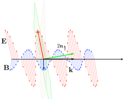
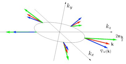
Figure 5: From Ref. Bisio2016 . (Colors online). Left: In a rectilinear polarized electromagnetic wave, the polarization plane (in green) is slightly tilted with respect the plane orthogonal to $\mathbf{k}$ (in gray). Right: vector $2\mathbf{n}_{\tfrac{\mathbf{k}}{2}}$ (in green), which is orthogonal to the polarization plane; wavevector $\mathbf{k}$ (in red) and group velocity (in blue) for the value $|\mathbf{k}|=0.8$ and different directions. Notice that the three vectors are not parallel (the angles between them depend on $\mathbf{k}$).

3.9.2 Vacuum dispersion

According to Eq. (41) the angular frequency of the electromagnetic waves is given by the modified dispersion relation

$$\omega(\mathbf{k})=2|\mathbf{n}_{\tfrac{\mathbf{k}}{2}}|,$$ (47)

which recovers the usual relation $\omega(\mathbf{k})=|\mathbf{k}|$ in the relativistic regime. In a dispersive medium, the speed of light is the group velocity $\nabla_{\mathbf{k}}\omega(\mathbf{k})$ of the electromagnetic waves, and Eq. (47) predict that the vacuum is dispersive, namely the speed of light generally depends on $\mathbf{k}$. Such dispersion phenomenon has been already analyzed in some literature on quantum gravity, where several authors considered how an hypothetical invariant length (corresponding to the Planck scale) could manifest itself in terms of modified dispersion relations ellis1992string ; lukierski1995classical ; Quantidischooft1996 ; amelino2001testable ; PhysRevLett.88.190403 . In these models the $\mathbf{k}$-dependent speed of light $c(\mathbf{k})$, at the leading order in $k:=|\mathbf{k}|$, is expanded as $c(\mathbf{k})\approx 1\pm\xi k^{\alpha}$, where $\xi$ is a numerical factor of the order $1$, while $\alpha$ is an integer. This is exactly what happens in our framework, where the intrinsic discreteness of the quantum cellular automata $A_{\mathbf{k}}^{\pm}$ leads to the dispersion relation of Eq. (47) from which one obtains the following $\mathbf{k}$-dependent speed of light

$$c^{\mp}(\mathbf{k})\approx 1\pm 3\frac{k_{x}k_{y}k_{z}}{|\mathbf{k}|^{2}}\approx 1\pm\tfrac{1}{\sqrt{3}}k.$$ (48)

Eq. (48) is obtained by evaluating the modulus of the group velocity and expanding in powers of $\mathbf{k}$ with the assumption $k_{x}=k_{y}=k_{z}=\tfrac{1}{\sqrt{3}}k$, ($k=|\mathbf{k}|$). Notice that the dispersion is not isotropic, and can also be superluminal, though uniformly bounded PhysRevA.90.062106 by a factor $\sqrt{d}$ (which coincides with the uniform bound of the quasi-isometric embedding). The prediction of dispersive behavior, as for the present automata theory of quantum fields, is especially interesting since it is experimentally falsifiable, and, as mentioned in Subsect. 3.8.3, allows to experimentally set the discreteness scale. In fact, differently to other birefringence effects (Fig.5), the disperision effect, although is extremely small in the relativistic regime, it accumulates and become magnified during a huge time of flight. For example, observations of the arrival times of pulses originated at cosmological distances (such as in some $\gamma$-ray burstsamelino1998tests ; abdo2009limit ; vasileiou2013constraints ; amelino2009prospects ), have sufficient sensitivity to detect corrections to the relativistic dispersion relation of the same order as in Eq. (48).

4 Recovering special relativity in a discrete quantum universe

We have seen how relativistic mechanics, and more precisely free QFT, can be recovered without using any mechanical primitive, and without making any use of special relativity, including the relativity principle itself. However, one may wonder how discreteness can be reconciled with Lorentz transformations, and most importantly, how the relativity principle itself can be restated in purely mathematical terms, without using the notions of space-time and inertial frame. In this section we will see how such goal can be easily accomplished.

The relativity principle is expressed by the statement:

1. Galileo’s Relativity Principle: The physical law is invariant with the inertial frame.

Otherwise stated: the physics that we observe, or, equivalently, its mathematical representation, is independent on the inertial frame that we use.

What is a frame? It is a mathematical representation of physical laws in terms of space and time coordinates. What is special about the inertial frame? A convenient way of answering is the following

1. Inertial frame: a reference frame where energy and momentum are conserved for an isolated system.

When a system is isolated? This is established by the theory. In classical mechanics, a system is isolated if there are no external forces acting on it. In quantum theory a system is isolated when its dynamical evolution is described by a unitary transformation on the system’s Hilbert space. At the very bottom of its notion, the inertial frame is the mathematical representation of the physical law that makes its analytical form the simplest. In classical physics, if we include the Maxwell equations among the invariant physical laws, what we get from Galileo’s principle is Einstein’s special relativity.

The quantum walk/automaton is an isolated system (it evolves unitarily). Mathematically the physical law that brings the information about the constants of the dynamics in terms of their Hilbert eigenspaces is provided by the eigenvalue equation. For the case of virtually Abelian group $G$ (which ultimately leads to physics in Euclidean space) the eigenvalue equation has the general form corresponding to Eqs. (19) and (21)

$$A_{\mathbf{k}}\psi(\omega,\mathbf{k})=e^{i\omega}\psi(\omega,\mathbf{k}),$$ (49)

with the eigenvalues usually collected into $s$ dispersion relations (the two functions $\omega^{\pm}(\mathbf{k})$ for the Weyl quantum walk). This translates into the following re-interpretation of representations of the eigenvalue equation:

1. Quantum-digital inertial frame: Representation in terms of eigen-spaces of the constants of the dynamics of the eigenvalue equation (49).

Using such notion of inertial frame, the principle of relativity is still the Galileo’s principle. The group of transformations that connect different inertial reference frames will be the quantum digital-version of the Poincaré group:

1. Quantum-digital Poincaré group: group of changes of representations in terms of eigenspaces of the dynamical constants that leave the eigenvalue equation (49) invariant.

It is obvious that the changes of representations make a group. Since the constants of dynamics are $\mathbf{k}$ and $\omega^{\pm}$, a change of representation corresponds to an invertible map $k\to k^{\prime}(k)$, where with $k$ we denote the four-vector $k:=(\omega,\mathbf{k})$.

In the following subsection we will see how the inherent discreteness of the algorithmic description leads to distortions of the Lorentz transformations, visible in principle at huge energies. Nevertheless, Einstein’s special relativity is perfectly recovered for $|\mathbf{k}|\ll 1$, namely at energy scales much higher than those ever tested.

On the other hand, as we will see in the following, discreteness has some plus compared to the continuum theory, since it contains the continuum theory as a special regime, and moreover it leads to some additional features with GR flavor: 1) it has a maximal particle mass with physical interpretation in terms of the Planck mass; 2) it leads to a De Sitter invariance (see Subsect. 4.2). And this, in addition to providing its own physical standards for space, time, and mass within a purely mathematical context (Subsect. 3.8.3).

4.1 Quantum-digital Poincaré group and the notion of particle

The eigenvalue equation (49) can now be rewritten in “relativistic notation” as follows

$$n_{\mu}(k)\sigma^{\mu}\psi(k)=0,$$ (50)

upon introducing the four-vectors

$$k=(\omega,\mathbf{k}),\quad n(k)=(\sin\omega,\mathbf{n}(\mathbf{k})),\quad\bm{\sigma}=(I,\mathbf{\sigma}),\quad\mathbf{\sigma}=(\sigma_{x},\sigma_{y},\sigma_{z}),$$ (51)

where the vector $\mathbf{n}(\mathbf{k})$ is defined in Eq. (16), namely

$$\mathbf{n}(\mathbf{k})\cdot\mathbf{\sigma}:=\frac{i}{2}(A_{\mathbf{k}}-A_{\mathbf{k}}^{\dagger}).$$ (52)

As already mentioned, since the constants of dynamics are $\mathbf{k}$ and $\omega^{\pm}$, a change of representation corresponds to a map $k\mapsto k^{\prime}(k)$. Now the principle of relativity corresponds to the requirement that the eigenvalue equation (50) is preserved under a change of representation. This means that the following identity must hold

$$n_{\mu}(k)\sigma^{\mu}=\tilde{\Gamma}^{-1}_{k}\,n_{\mu}(k^{\prime})\sigma^{\mu}\,\Gamma_{k},$$ (53)

where $\Gamma_{k}$, $\tilde{\Gamma}_{k}$ are invertible matrices representing the change of representation.

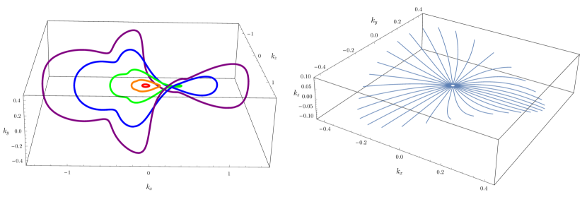
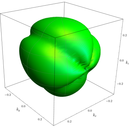
Figure 6: From Ref. lrntz3d . (Colors online). The distortion effects of the Lorentz group in the present quantum walk theory leading to the Weyl quantum field in the relativistic limit. Top left figure: the orbit of the wavevectors $\mathbf{k}=(k_{x},0,0)$, with $k_{x}\in\{.05,.2,.5,1,1.7\}$ under the rotation around the $z$ axis. Top right figure: the orbit of wavevectors with $|\mathbf{k}|=0.01$ for various directions in the $(k_{x},k_{y})$ plane under the boosts with ${\mathbf{\beta}}$ parallel to $\mathbf{k}$ and $|{\mathbf{\beta}}|\in[0,\tanh 4]$. Bottom figure: the orbit of the wavevector $\mathbf{k}=(0.3,0,0)$ under the full rotation group $SO(3)$.

The simplest example of change of observer is the one given by the trivial relabeling $k^{\prime}=k$ and by the matrices $\Gamma_{k}=\tilde{\Gamma}_{k}=e^{i\lambda(\mathbf{k})}$, where $\lambda(\mathbf{k})$ is an arbitrary real function of $\mathbf{k}$. When $\lambda(\mathbf{k})$ is a linear function we recover the usual group of translations. The set of changes of representation $k\mapsto k^{\prime}(k)$ for which Eq. (53) holds are a group, which is the largest group of symmetries of the dynamics. In covariant notation the dispersion relations are rewritten as follows

$$n_{\mu}^{\pm}(k)n^{\mu\pm}(k)=0,$$ (54)

and in the small wave-vector regime one has $n(k)\sim k$, recovering the usual relativistic dispersion relation.

In addition to the neighbour of the wavevector $\mathbf{k_{0}}=(0,0,0)$, the Weyl equations can be recovered from the quantum walk (16) also in the neighborhood of the wavevectors in Eq. (15). The mapping between the vectors $\mathbf{k}_{i}$ exchange chirality of the particle and double the particles to four species in total: two left-handed and two right-handed. In the following we will therefore more generally refer to the relativistic regime as the neighborhoods of the vectors $\{\mathbf{k}_{i}\}_{i=0}^{3}$.

The group of symmetries of the dynamics of the quantum walks (16) contains a nonlinear representation of the Poincaré group, which exactly recovers the usual linear one in the relativistic regime. For any arbitrary non vanishing function $f(k)$ one introduces the four-vector

$$p^{(f)}=\mathcal{D}^{(f)}(k):=f(k)n(k)$$ (55)

and rewrite the eigenvalue equation (50) as follows

$$p^{(f)}_{\mu}\sigma^{\mu}\psi(k)=0.$$ (56)

Upon denoting the usual Lorentz transformation by $L_{\mathbf{\beta}}$ for a suitable $f$ lrntz3d the Brillouin zone splits into four regions $\mathsf{B}_{i}$, $i=1,\ldots,4$ centered around $\mathbf{k}_{i}$ $i=0,\ldots 3$, such that the composition

$$\mathcal{L}^{(f)}_{\mathbf{\beta}}:=\mathcal{D}^{(f)-1}L_{\mathbf{\beta}}\mathcal{D}^{(f)}$$ (57)

is well defined on each region separately. The four invariant regions corresponding to the four different massless Fermionic particles show that the Wigner notion of ”particle” as invariant of the Poincaré group survives in a discrete world. For fixed function $f$ the maps $\mathcal{L}^{(f)}_{\mathbf{\beta}}$ provide a non-linear representation of the Lorentz group amelino2001planck ; amelino2002relativity ; magueijo2002lorentz . In Figs. 6 the orbits of some wavevectors under subgroups of the nonlinear Lorentz group are reported. The distortion effects due to underlying discreteness are evident at large wavevectors and boosts. The relabeling $k\rightarrow k^{\prime}(k)=\mathcal{L}^{(f)}_{\mathbf{\beta}}(k)$ satisfies Eq. (53) with $\Gamma_{k}=\Lambda_{\mathbf{\beta}}$ and $\tilde{\Gamma}_{k}=\tilde{\Lambda}_{\mathbf{\beta}}$ for the right-handed particles, and $\Gamma_{k}=\tilde{\Lambda}_{\mathbf{\beta}}$ and $\tilde{\Gamma}_{k}=\Lambda_{\mathbf{\beta}}$ for the left-handed particles, with $\Lambda_{\mathbf{\beta}}$ and $\tilde{\Lambda}_{\mathbf{\beta}}$ being the $(0,\tfrac{1}{2})$ and $(\tfrac{1}{2},0)$ representation of the Lorentz group, independently on $k$ in each pertaining region.

For varying $f$, one obtains a much larger group, including infinitely many copies of the nonlinear Lorentz one. In the small wave-vector regime the whole group collapses to the usual linear Lorentz group for each particle.

4.2 De Sitter group for nonvanishing mass

Up to now we have analyzed what happens with massless particles. For massive particles described by the Dirac walk (22), the rest-mass $m$ gets involved into the frame transformations, and their group becomes a nonlinear realization of the De Sitter group $SO(1,4)$ with infinite cosmological constant, where the rest mass $m$ of the particle plays the role of the additional coordinate. One recovers the previous nonlinear Lorentz group at the order $\mathcal{O}(m^{2})$.

5 Conclusions and future perspectives: the interacting theory, …, gravity?

The logical connections that have lead us to build up our quantum-walk theory of fields leading to free QFT are summarized in Fig. 7.

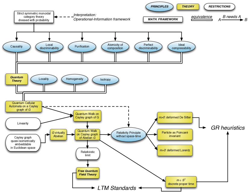
Figure 7: Logical scheme of the derivation from principles of the present quantum-walk theory of fields, with the known free quantum field theory as its relativistic limit. The top six principles from which quantum theory of abstract system is derived are not discussed in the present paper, and can be found in Refs. chiribella2011informational ; QTfromprinciples .

The free relativistic quantum field theory emerges as a special regime (the relativistic regime) of the evolution of countably many Fermionic quantum bits, provided that their unitary interactions satisfy the principles of homogeneity, locality, and isotropy, and with the restrictions of linearity of the evolution and of quasi-isometric embedding of the graph of interaction in an Euclidean space.

We are left now with the not easy task of recovering also the interacting relativistic quantum field theory, where particles are created and annihilated. We will need to devise which additional principles are missing that will lead to the interacting theory, breaking the linearity assumption. This is likely to be related to the nature of a gauge transformation. How can this be restated in terms of a new principle? From the point of view of a free theory, the interaction can be viewed as a violation of homogeneity, corresponding to the presence of another interacting field–namely the gauge-field. The gauge-field can be regarded as a restoration of homogeneity by a higher level homogeneous “meta-law”. For example, one can exploit the arbitrariness of the local bases of the Hilbert block subspaces $\mathbb{C}^{s}$ for the Weyl automata, having the bases dependent on the local value of the wave-function of the gauge automaton made with pairs of entangled Fermions, as for the Maxwell automaton. In order to keep the interaction local, one can consider an on-situ interaction. In such a way one would have a quantum ab initio gauge theory, without the need of artificially quantizing the gauge fields, nor of introducing mechanical Lagrangians. A $d=1$ interacting theory of the kind of a Fermionic Hubbard quantum cellular automaton, has been very recently analytically investigated by the Bethe ansatz Hubbard , and two-particle bound states have been established. It should be emphasized that for $d=3$ just the possibility of recovering QED in the relativistic regime would be very interesting, since it will provide a definite procedure for renormalization. Very interesting will be also the analysis of the full dynamical invariance group, leading also to a nonlinear version of the Poincaré group, with the possibility that this restricts the choice of the function $f$ in Eq. (55). Studying the full symmetry group of the interacting theory will also have the potential of providing additional internal symmetries, e. g. the $SU(3)$ symmetry group of QCD, with the Fermion doubling possibly playing the role in adding physical particles. The mass as a variable quantum observable (as in Subsections 3.8.2 and 4.2) may provide rules about the lifetimes of different species of particles. The additional quasi-static scalar mode entering in the tensor-product of the two Weyl automata that give the Maxwell field in Subsect. 3.9 may turn out to play a role in the interacting theory, e. g. playing the role of a Higg boson providing the mass value, or even being pivotal for gravitation. But for now we are just in the realm of speculations.

What we can say for sure is that it is not just a coincidence that so much physics comes out from so few general principles. How amazing is the whole resulting theory which, in addition to having a complete logical coherence by construction, it also winks at GR through the two nontrivial features of the maximum mass, and the De Sitter invariance. And with special relativity derived without space-time and kinematics, in a fully quantum ab initio theory. So much from so little? This is the power of the new information-theoretical paradigm.

Appendices

Appendix A A very brief historical account

The first very preliminary heuristic ideas about the current quantum cellular automaton/quantum walk theory have been presented in a friendly and open-minded environment at Perimeter Institute in Waterloo in a series of three talks in 2010-11 darianopirsa-GUT1 ; darianopirsa-GUT2 ; darianopirsa-GUT3 . Originally, the idea of foliations over the quantum circuit has been explored, showing how the Lorentz time-dilations and space-contractions emerge by changing the foliation. This work has lead to the analyses of Alessandro Tosini in Refs. d2010space ; d2011emergence and in the conclusive work d2013emergence . However, it was soon realized that the foliation on the quantum circuit explores only the causal connectivity of the automaton, and works in the same way also for a classical circuit, as it happens for random walks in one dimension (see e. g. Ref. stein1996concept ). Moreover, only rational boosts can be used, with the additional artifact that the events have to be coarse-grained in a boost-dependent way, with very different coarse-graining for very close values of the boost. This makes the recovery of the usual Lorentz transformations at large scales practically unfeasible. On the other hand, the first Dirac automaton in one space dimension mauro2012quantum exhibited perfect Lorentz covariance for small wavevectors, which made clear that the quantum nature of the circuit plays a pivotal role in recovering the Lorentz invariance. In the same Ref. mauro2012quantum it also emerged that the Dirac mass has to be upper bounded as a consequence of unitarity.

The idea that so-called “conventional”principles as homogeneity and isotropy may play a special role entered the scene since the very beginning darianopirsa-GUT1 through the connection with the old works of Ignatowsky von1910einige , whereas ideas about how to treat gauge theories emerged already in Ref. darianopirsa-GUT3 . However, the project remained stuck for a couple of years because of two dead ends. First, we were looking to the realization of the quantum cellular automaton in terms of circuit gates, and we much later realized that the problem of connecting the gate realization (socalled Margolus scheme toffoli1987cellular ) to the linear quantum walk was a highly non trivial problem for dimension greater than one. Second, we where considering Jordan-Wigner mappings between local qubits and discrete Fermions darianosaggiatore , generalizing to dimensions $d>1$ what can be done for d=1, and later Tosini realized that for $d>1$ such mapping cannot be done iso-locally IJMP14 ; EPL14 , namely preserving the locality of interactions. Paolo Perinotti, inspired from the work of Bialynicki-Birula bialynicki1994weyl , recognized the first Dirac quantum walks in 2 and 3 dimensions. Later the graph structure of the walk was pointed out to be a Cayley graph of a group by Matt Brin, and the work of the derivation from principles of Weyl and Dirac PhysRevA.90.062106 followed after a Paolo’s nontrivial solution of the unitarity conditions. This was the turning point of the whole program. It was soon recognized that the Maxwell field could be obtained by tensor product of two Weyl, and Alessandro Bisio soon found a way of achieving the photons with entangled pairs of Fermions. We finally realized the pivotal role played by the eigenvalue equation of the quantum in restating the relativity principle and recovering Lorentz covariance, and Bisio found the construction recovering the notion of particle as invariant of the deformed Poincaré group.

Appendix B My encounter with David Ritz Finkelstein

Vieque Island, January 6th 2014: FQXi IV International Conference on The Physics of Information. The conference is very interactive, mostly devoted to debates, round tables, and working groups. Max Tagmark organizes and chaires a morning session made of five-minutes talks. The audience includes distinguished scientists, a unique opportunity for presenting my Templeton project A Quantum-Digital Universe. I want to say many things that I consider very important, and I prepare my talk carefully, measuring the time of each single sentence, and memorizing each single word. The result goes beyond my best expectations, with gratifying comments by a number of scientists, some whom I meet for the first time. But the best that happens is that a beautiful old man, whom I never met before, with a white bear and a hat, literally embraces me with a great smile, and almost with tears in his blue eyes says that I realized one of his dreams. His enthusiasm, so passionate and authentic captures me. I spend most of the following days discussing with him. He invites me to visit him in his home in Atlanta.

I visit David on March 16th and 17th in a weekend during a visit in Boston. His house is beautiful, with large windows opened on a surrounding forest. With his wife Shlomit we have pleasant conversations, some about their past encounter with the Dalai Lama.

David writes a nice dedication on my copy of his last book finkelstein2012quantumc . He then asks me to explain to him the derivation of quantum theory from information-theoretical principles (which I did with my former students Paolo Perinotti and Giulio Chiribella chiribella2011informational : a textbook from Cambridge University Press is now in press QTfromprinciples ). I spend almost the two entire days in front of a small blackboard in David room full of books (see Fig. 8), drawing diagrams and answering to his many questions. His genuine interest will boost my enthusiasm for the years to come.

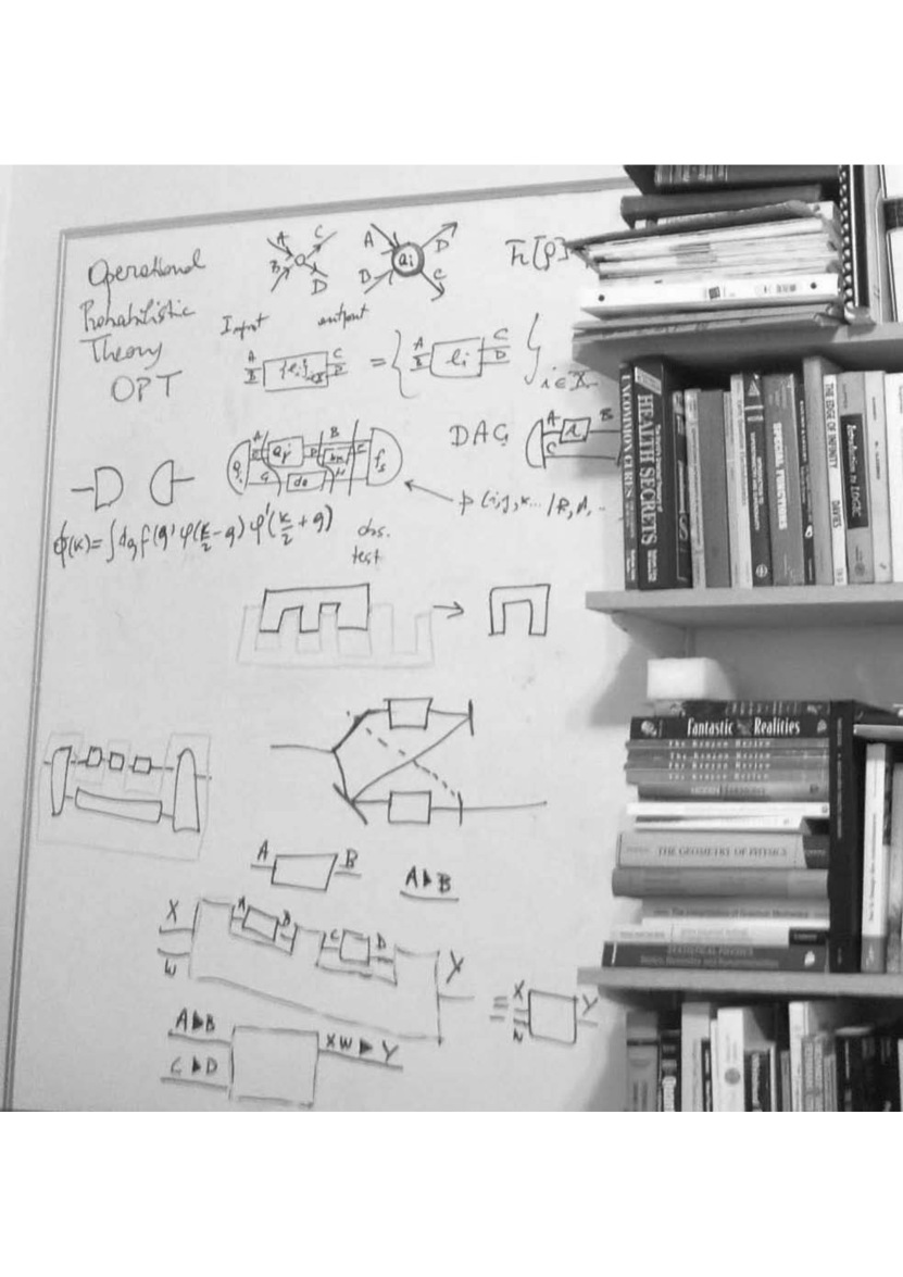
Figure 8: The blackboard in David room, after a day-long tour on the derivation of quantum theory from principles QTfromprinciples . You can notice some diagrams that pertain noncausal variations of quantum theory.

After that visit David and I will continue to exchange emails. David regularly will send to me updates of his work. We promise to exchange visits soon, but unfortunately this will not happen again.

Appendix C My talk at FQXi 2014 verbatim

I’d like to tell you about the astonishing power of taking information more fundamental than matter, the informational paradigm advocated by Wheeler, Feynman, and Seth Lloyd of “the universe as a huge quantum computer”. Quantum Theory is indeed a theory of information, since it can be axiomatically derived from six axioms of pure information-theoretical nature. Five of the postulates are in common with classical information. The one that discriminates between quantum and classical is the principle of conservation of information–technically the purification postulate. Information means describing everything in terms of input-output relations between events/transformations, mathematically associating probabilities to closed circuits between preparations and observations. [Some of the principles are conceptually quite new and interesting, such as the local discriminability one, which in the quantum case reconciles holism with reductionism, with the possibility of achieving complete information by local observation.]

Now these postulates provide only the quantum theory of abstract systems, not the mechanical part of the theory. In order to get this you need to add new principles that lead to quantum field theory, without assuming relativity and space-time. These principles describe the topology of interactions, which determine the flow of information along the circuit. The first of these requirements is that of finite info-density, corresponding to having a numerable set of finite-dimensional quantum systems in interaction. Such principle, along with the assumption of unitarity, locality, homogeneity, isotropy and minimal dimension of the systems in interaction, are equivalent to minimizing the quantum algorithmic complexity of the information processing, reducing the physical law to a bunch of few quantum gates, and leading to a description in terms of a Quantum Cellular Automaton.

Now, it turns out that from these few assumptions only two quantum cellular automata follow that are connected by CPT, and Lorentz covariance is broken. They both converge to the Dirac equation in the relativistic limit of small masses and small wave-vectors. In the ultra-relativistic limit of large wave-vectors or masses (corresponding to a Planck scale) Lorentz covariance becomes only an approximate symmetry, and one has an energy scale and length scale that are invariant in addition to the speed of light, corresponding to the Doubly Special Relativity of Amelino-Camelia/Smolin/Magueijo, with the phenomenon of relative locality, namely that also coincidence in space, not only in time, is observer-dependent. The covariance is given by the group of transformation leaving the dispersion relations of the automaton invariant, and holds for energy-momentum. When you get back to space-time via Fourier, then you recover a space-time of quantum nature, with space-time points in superposition.

The quantum cellular automaton can be regarded as a theory unifying scales ranging from Planck to Fermi. It is interesting to notice that the same quantum cellular automaton also gives the Maxwell field, interestingly in the form of the de Broglie-Fermi neutrino theory of the photon. With the principle of bounded information density, also the Boson becomes an emergent notion, but the relation with Fermions is subtle in terms of localization. The fact that the theory is discrete avoids all problems that plague quantum field theory arising from the continuum, especially the problem of localization, but, most relevant, the theory is quantum ab initio, with no need of quantization rules. And this is the great bonus of taking information as more fundamental than matter.

- (1) G. Chiribella, G.M. D’Ariano, P. Perinotti, Phys. Rev. A 84, 012311 (2011)
- (2) G.M. D’Ariano, G. Chiribella, P. Perinotti, Quantum Theory from First Principles (Cambridge University Press, Cambridge, 2017). In press
- (3) G.M. D’Ariano, P. Perinotti, Phys. Rev. A 90, 062106 (2014)
- (4) A. Bisio, G.M. D’Ariano, A. Tosini, Phys. Rev. A 88, 032301 (2013)
- (5) A. Bisio, G.M. D’Ariano, A. Tosini, Annals of Physics 354, 244 (2015)
- (6) A. Bisio, G.M. D’Ariano, P. Perinotti, Annals of Physics 368, 177 (2016)
- (7) L. Susskind, Journal of Mathematical Physics 36, 6377 (1995)
- (8) R. Bousso, Reviews of Modern Physics 74, 825 (2002)
- (9) J.V. Neumann, Mathematical foundations of quantum mechanics. 2 (Princeton university press, 1955)
- (10) G. Chiribella, G.M. D’Ariano, P. Perinotti, in Quantum Theory: Informational Foundations and Foils, ed. by G. Chiribella, R. Spekkens (Springer, 2016), pp. 165–175
- (11) G.M. D’Ariano, P. Perinotti, Found. Phys. 46, 269 (2016)
- (12) H. Halvorson, R. Clifton, Philosophy of Science 69, 1 (2002)
- (13) M. Kuhlmann, Scientific American 24, 84 (2015)
- (14) A. Bisio, G.M. D’Ariano, P. Perinotti, A. Tosini, Found. Phys. 45, 1137 (2015)
- (15) A. Bisio, G.M. D’Ariano, P. Perinotti, A. Tosini, Found. Phys. 45, 1203 (2015)
- (16) G.M. D’Ariano, Phys. Lett. A 376(5), 697 (2012)
- (17) A. Bisio, G.M. D’Ariano, P. Perinotti, arXiv preprint arXiv:1503.01017v3 (2015)
- (18) G.M. D’Ariano, P. Perinotti, Front. Phys. 12, 120301 (2017). DOI 10.1007/s11467-016-0616-z. Special Topic: Quantum Communication, Measurement, and Computing, in press (arXiv:1608.02004)
- (19) G.M. D’Ariano, M. Erba, P. Perinotti, A. Tosini, arXiv preprint arXiv:1511.03992 (2015)
- (20) A.J. Hey, Feynman and Computation-Exploring the Limits of Computers (Perseus Books, 1998)
- (21) S.B. Bravyi, A.Y. Kitaev, Annals of Physics 298, 210 (2002)
- (22) G.M. D’Ariano, F. Manessi, P. Perinotti, A. Tosini, Int. J. Mod. Phys. A 17, 1430025 (2014)
- (23) G.M. D’Ariano, F. Manessi, P. Perinotti, A. Tosini, Europhysics Letters 107, 20009 (2014)
- (24) R.G. Colodny (ed.), From quarks to quasars: philosophical problems of modern physics (University of Pittsburgh Pre, 1986)
- (25) P. de La Harpe, Topics in geometric group theory (University of Chicago Press, 2000)
- (26) B. Farb, private communication
- (27) C. Drutu, private communication
- (28) R. Tessera, private communication
- (29) G.M. D’Ariano, M. Erba, P. Perinotti, unpublished
- (30) M. Kapovich, unpublished
- (31) G.W. Mackey, American Journal of Mathematics 73, 576 (1951)
- (32) G.W. Mackey, Annals of Mathematics 55, 101 (1952)
- (33) G.W. Mackey, Annals of Mathematics 58, 193 (1953)
- (34) G.M. D’Ariano, N. Mosco, P. Perinotti, A. Tosini, Entropy 18, 228 (2016)
- (35) G.M. D’Ariano, N. Mosco, P. Perinotti, A. Tosini, Phys. Lett. A 378 (2014)
- (36) G.M. D’Ariano, N. Mosco, P. Perinotti, A. Tosini, EPL 109 (2015)
- (37) G.M. D’Ariano, N. Mosco, P. Perinotti, A. Tosini, (2015). Discrete Feynman propagator for the Weyl quantum walk in 3+1 dimensions
- (38) L.H. Kauffman, H.P. Noyes, Physics Letters A 218(3), 139 (1996)
- (39) D.M. Greenberger, Journal of Mathematical Physics 11(8), 2329 (1970)
- (40) J. Ellis, N. Mavromatos, D.V. Nanopoulos, Physics Letters B 293(1), 37 (1992)
- (41) J. Lukierski, H. Ruegg, W.J. Zakrzewski, Annals of Physics 243(1), 90 (1995)
- (42) G. ’t Hooft, Class. Quantum Grav. 13(5), 1023 (1996)
- (43) G. Amelino-Camelia, Physics Letters B 510(1), 255 (2001)
- (44) J. Magueijo, L. Smolin, Phys. Rev. Lett. 88, 190403 (2002)
- (45) G. Amelino-Camelia, J. Ellis, N. Mavromatos, D.V. Nanopoulos, S. Sarkar, Nature 393(6687), 763 (1998)
- (46) A. Abdo, M. Ackermann, M. Ajello, K. Asano, W. Atwood, M. Axelsson, L. Baldini, J. Ballet, G. Barbiellini, M. Baring, et al., Nature 462(7271), 331 (2009)
- (47) V. Vasileiou, A. Jacholkowska, F. Piron, J. Bolmont, C. Couturier, J. Granot, F.W. Stecker, J. Cohen-Tanugi, F. Longo, Physical Review D 87(12), 122001 (2013)
- (48) G. Amelino-Camelia, L. Smolin, Physical Review D 80(8), 084017 (2009)
- (49) A. Bibeau-Delisle, A. Bisio, G.M. D’Ariano, P. Perinotti, A. Tosini, EPL (2015). In press
- (50) A. Bisio, G.M. D’Ariano, P. Perinotti, Phil. Trans. R. Soc. A 374 (2016)
- (51) L. Susskind, Phys. Rev. D 16, 3031 (1977)
- (52) G. Amelino-Camelia, T. Piran, Physical Review D 64(3), 036005 (2001)
- (53) G. Amelino-Camelia, International Journal of Modern Physics D 11(01), 35 (2002)
- (54) J. Magueijo, L. Smolin, Physical Review Letters 88(19), 190403 (2002)
- (55) (2012)
- (56) G.M. D’Ariano, A computational grand-unified theory (2010). URL:http://pirsa.org/10020037
- (57) G.M. D’Ariano, Physics as information: Quantum theory meets relativity (2010). Http://pirsa.org/10110080
- (58) G.M. D’Ariano, A quantum-digital universe (2011). Http://pirsa.org/11050042
- (59) G.M. D’Ariano, in Quantum Theory: Reconsideration of Foundations 5, vol. CP1232 (AIP, 2010), vol. CP1232, p. 3
- (60) G.M. D’Ariano, in Advances in Quantum Theory, vol. CP1327 (AIP, 2011), vol. CP1327, p. 7
- (61) G.M. D’Ariano, in Foundations of Probability and Physics - 6, vol. CP1508 (AIP, 2012), vol. CP1508, p. 146
- (62) G.M. D’Ariano, in Foundations of Probability and Physics - 6, vol. CP1424 (AIP, 2012), vol. CP1424, p. 371
- (63) G.M. D’Ariano, in Quantum Communication, measurement and Computing (QCMC), vol. CP1363 (AIP, 2011), vol. CP1363, p. 63
- (64) G. D’Ariano, FQXi Essay Contest: Is Reality Digital or Analog? (2011)
- (65) G. D’Ariano, FQXi Essay Contest: Questioning the Foundations: Which of Our Basic Physical Assumptions Are Wrong? (2012)
- (66) G. D’Ariano, FQXi Essay Contest: It From Bit or Bit From It? (2013)
- (67) G. D’Ariano, FQXi Essay Contest: Trick or Truth: the Mysterious Connection Between Physics and Mathematics (2013)
- (68) G.M. D’Ariano, Adv. Sci. Lett. 17, 130 (2012)
- (69) G.M. D’Ariano, in Questioning the Foundations of Physics, The Frontiers Collection, ed. by A.A. et al. (Springer, 2015), pp. 165–175
- (70) G.M. D’Ariano, in It From Bit or Bit From It?, The Frontiers Collection, ed. by A.A. et al. (Springer, 2015), pp. 25–35
- (71) G.M. D’Ariano, La Recherche 489, 48 (2014)
- (72) G.M. D’Ariano, A. Tosini, arXiv preprint arXiv:1008.4805 (2010)
- (73) G.M. D’Ariano, A. Tosini, arXiv preprint arXiv:1109.0118 (2011)
- (74) G.M. D’Ariano, A. Tosini, Studies in History and Philosophy of Science Part B: Studies in History and Philosophy of Modern Physics 44(3), 294 (2013)
- (75) I. Stein, The concept of object as the foundation of physics (Peter Lang, 1996)
- (76) W. von Ignatowsky, Verh. Deutsch. Phys. Ges 12, 788 (1910)
- (77) T. Toffoli, N. Margolus, Cellular automata machines (MIT press, 1987)
- (78) G.M. D’Ariano, Il Nuovo Saggiatore 28, 13 (2012)
- (79) I. Bialynicki-Birula, Physical Review D 49(12), 6920 (1994)
- (80) D.R. Finkelstein, Quantum relativity: a synthesis of the ideas of Einstein and Heisenberg (Springer Science & Business Media, 2012)