A Tutorial on Modeling and Analysis of Dynamic Social Networks. Part I

Abstract

In recent years, we have observed a significant trend towards filling the gap between social network analysis and control. This trend was enabled by the introduction of new mathematical models describing dynamics of social groups, the advancement in complex networks theory and multi-agent systems, and the development of modern computational tools for big data analysis. The aim of this tutorial is to highlight a novel chapter of control theory, dealing with applications to social systems, to the attention of the broad research community. This paper is the first part of the tutorial, and it is focused on the most classical models of social dynamics and on their relations to the recent achievements in multi-agent systems.

1 Introduction

The 20th century witnessed a crucial paradigm shift in social and behavioral sciences, which can be described as “moving from the description of social bodies to dynamic problems of changing group life” [1]. Unlike individualistic approaches, focused on individual choices and interests of social actors, the emerging theories dealt with structural properties of social groups, organizations and movements, focusing on social relations (or ties) among their members.

A breakthrough in the analysis of social groups was enabled by introducing a quantitative method for describing social relations, later called sociometry [2, 3]. The pioneering work [2] introduced an important graphical tool of sociogram, that is, “a graph that visualizes the underlying structure of a group and the position each individual has within it” [2]. The works [2, 3] also broadly used the term “network”, meaning a group of individuals that are “bound together” by some long-term relationships. Later, the term social network was coined, which denotes a structure, constituted by social actors (individuals or organizations) and social ties among them. Sociometry has given birth to the interdisciplinary science of Social Network Analysis (SNA) [4, 5, 6, 7], extensively using mathematical methods and algorithmic tools to study structural properties of social networks and social movements [8]. SNA is closely related to economics [9, 10], political studies [11], medicine and health care [12]. The development of SNA has inspired many important concepts of modern network theory  [13, 14, 15] such as e.g. cliques and communities, centrality measures, small-world network, graph’s density and clustering coefficient.

On a parallel line of research, Norbert Wiener introduced the general science of Cybernetics [16, 17] with the objective to unify systems, control and information theory. Wiener believed that this new science should become a powerful tool in studying social processes, arguing that “society can only be understood through a study of the messages and communication facilities which belong to it” [17]. Confirming Wiener’s ideas, the development of social sciences in the 20th century has given birth to a new chapter of sociology, called “sociocybernetics” [18] and led to the increasing comprehension that “the foundational problem of sociology is the coordination and control of social systems” [19]. However, the realm of social systems has remained almost untouched by modern control theory in spite of the tremendous progress in control of complex large-scale systems [20, 21, 22].

The gap between the well-developed theory of SNA and control can be explained by the lack of mathematical models, describing social dynamics, and tools for quantitative analysis and numerical simulation of large-scale social groups. While many natural and engineered networks exhibit “spontaneous order” effects [23] (consensus, synchrony and other regular collective behaviors), social communities are often featured by highly “irregular” and sophisticated dynamics. Opinions of individuals and actions related to them often fail to reach consensus but rather exhibit persistent disagreement, e.g. clustering or cleavage [19]. This requires to develop mathematical models that are sufficiently “rich” to capture the behavior of social actors but are also “simple” enough to be rigorously analyzed. Although various aspects of “social” and “group” dynamics have been studied in the sociological literature [1, 24], mathematical methods of SNA have focused on graph-theoretic properties of social networks, paying much less attention to dynamics over them. The relevant models have been mostly confined to very special processes, such as e.g. random walks, contagion and percolation [14, 15].

The recent years have witnessed an important tendency towards filling the gap between SNA and dynamical systems, giving rise to new theories of Dynamical Social Networks Analysis (DSNA) [25] and temporal or evolutionary networks [26, 27]. Advancements in statistical physics have given rise to a new science of sociodynamics [28, 29], which stipulates analogies between social communities and physical systems. Besides theoretical methods for analysis of complex social processes, software tools for big data analysis have been developed, which enable an investigation of Online Social Networks such as Facebook and Twitter and dynamical processes over them [30].

Without any doubt, applications of multi-agent and networked control to social groups will become a key component of the emerging science on dynamic social networks. Although the models of social processes have been suggested in abundance [31, 29, 32, 33, 19], only a few of them have been rigorously analyzed from the system-theoretic viewpoint. Even less attention has been paid to their experimental validation, which requires to develop rigorous identification methods. A branch of control theory, addressing problems from social and behavioral sciences, is very young, and its contours are still blurred. Without aiming to provide a complete and exhaustive survey of this novel area at its dawn, this tutorial focuses on the most “mature” dynamic models and on the most influential mathematical results, related to them. These models and results are mainly concerned with opinion formation under social influence.

This paper, being the first part of the tutorial, introduces preliminary mathematical concepts and considers the four models of opinion evolution, introduced in 1950-1990s (but rigorously examined only recently): the models by French-DeGroot, Abelson, Friedkin-Johnsen and Taylor. We also discuss the relations between these models and modern multi-agent control, where some of them have been subsequently rediscovered. In the second part of the tutorial more advanced models of opinion evolution, the current trends and novel challenges for systems and control in social sciences will be considered.

The paper is organized as follows. Section 2 introduces some preliminary concepts, regarding multi-agent networks, graphs and matrices. In Section 3 we introduce the French-DeGroot model and discuss its relation to multi-agent consensus. Section 4 introduces a continuous-time counterpart of the French-DeGroot model, proposed by Abelson; in this section the Abelson diversity problem is also discussed. Sections 5 and 6 introduce, respectively, the Taylor and Friedkin-Johnsen models, describing opinion formation in presence of stubborn and prejudiced agents.

2 Opinions, Agents, Graphs and Matrices

In this section, we discuss several important concepts, broadly used throughout the paper.

2.1 Approaches to opinion dynamics modeling

In this tutorial, we primarily deal with models of opinion dynamics. As discussed in [19], individuals’ opinions stand for their cognitive orientations towards some objects (e.g. particular issues, events or other individuals), for instance, displayed attitudes [34, 35, 36] or subjective certainties of belief [37]. Mathematically, opinions are just scalar or vector quantities associated with social actors.

Up to now, system-theoretic studies on opinion dynamics have primarily focused on models with real-valued (“continuous”) opinions, which can attain continuum of values and are treated as some quantities of interest, e.g. subjective probabilities [38, 39]. These models obey systems of ordinary differential or difference equations and can be examined by conventional control-theoretic techniques. A discrete-valued scalar opinion is often associated with some action or decision taken by a social actor, e.g. to support some movement or abstain from it and to vote for or against a bill [29, 40, 41, 42, 43, 44, 45]. A multidimensional discrete-valued opinion may be treated as a set of cultural traits [46]. Analysis of discrete-valued opinion dynamics usually require techniques from advanced probability theory that are mainly beyond the scope of this tutorial.

Models of social dynamics can be divided into two major classes: macroscopic and microscopic models. Macroscopic models of opinion dynamics are similar in spirit to models of continuum mechanics, based on Euler’s formalism; this approach to opinion modeling is also called Eulerian [47, 48] or statistical [40]. Macroscopic models describe how the distribution of opinions (e.g. the vote preferences on some election or referendum) evolves over time. The statistical approach is typically used in “sociodynamics” [28] and evolutionary game theory [49, 9] (where the “opinions” of players stand for their strategies); some of macroscopic models date back to 1930-40s [50, 51].

Microscopic, or agent-based, models of opinion formation describes how opinions of individual social actors, henceforth called agents, evolve. There is an analogy between the microscopic approach, also called aggregative [52], and the Lagrangian formalism in mechanics [47]. Unlike statistical models, adequate for very large groups (mathematically, the number of agents goes to infinity), agent-based models can describe both small-size and large-scale communities.

With the aim to provide a basic introduction to social dynamics modeling and analysis, this tutorial is confined to agent-based models with real-valued scalar and vector opinions, whereas other models are either skipped or mentioned briefly. All the models, considered in this paper, deal with an idealistic closed community, which is neither left by the agents nor can acquire new members. Hence the size of the group, denoted by $n\geq 2$, remains unchanged.

2.2 Basic notions from graph theory

Social interactions among the agents are described by weighted (or valued) directed graphs. We introduce only basic definitions regarding graphs and their properties; a more detailed exposition and examples of specific graphs can be found in textbooks on graph theory, networks or SNA, e.g. [53, 54, 4, 9, 10, 55]. The reader familiar with graph theory and matrix theory may skip reading the remainder of this section.

Henceforth the term “graph” strands for a directed graph (digraph), formally defined as follows.

Definition 1

(Graph) A graph is a pair $\mathcal{G}=(V,E)$, where $V=\{v_{1},\ldots,v_{n}\}$ and $E\subseteq V\times V$ are finite sets. The elements $v_{i}$ are called vertices or nodes of $\mathcal{G}$ and the elements of $E$ are referred to as its edges or arcs.

Connections among the nodes are conveniently encoded by the graph’s adjacency matrix $A=(a_{ij})$. In graph theory, the arc $(i,j)$ usually corresponds to the positive entry $a_{ij}>0$. In multi-agent control [56, 57] and opinion formation modeling it is however convenient to identify the arc $(i,j)$ with the entry $a_{ji}>0$.

Definition 2

(Adjacency matrix) Given a graph $\mathcal{G}=(V,E)$, a nonnegative matrix $A=(a_{ij})_{i,j\in V}$ is adapted to $\mathcal{G}$ or is a weighted adjacency matrix for $\mathcal{G}$ if $(i,j)\in E$ when $a_{ji}>0$ and $(i,j)\not\in E$ otherwise.

Definition 3

(Weighted graph) A weighted graph is a triple $\mathcal{G}=(V,E,A)$, where $(V,E)$ is a graph and $A$ is a weighted adjacency matrix for it.

Any graph $(V,E)$ can be considered as a weighted graph by assigning to it a binary adjacency matrix

$$A=(a_{ij})_{i,j\in V},\quad a_{ij}=\begin{cases}1,\quad(j,i)\in E\\ 0,\quad\text{otherwise}.\end{cases}$$

On the other hand, any nonnegative matrix $A=(a_{ij})_{i,j\in V}$ is adapted to the unique graph $\mathcal{G}[A]=(V,E[A],A)$. Typically, the nodes are in one-to-one correspondence with the agents and $V=\{1,\ldots,n\}$.

Definition 4

(Subgraph) The graph $\mathcal{G}=(V,E)$ contains the graph $\mathcal{G}^{\prime}=(V^{\prime},E^{\prime})$, or $\mathcal{G}^{\prime}$ is a subgraph of $\mathcal{G}$, if $\emptyset\neq V^{\prime}\subseteq V$ and $E^{\prime}\subseteq(V^{\prime}\times V^{\prime})\cap E$.

Simply speaking, the subgraph is obtained from the graph by removing some arcs and some nodes.

Definition 5

(Walk) A walk of length $k$ connecting node $i$ to node $i^{\prime}$ is a sequence of nodes $i_{0},\ldots,i_{k}\in V$, where $i_{0}=i$, $i_{k}=i^{\prime}$ and adjacent nodes are connected by arcs: $(i_{s-1},i_{s})\in E$ for any $s=1,\ldots,k$. A walk from a node to itself is a cycle. A trivial cycle of length $1$ is called a self-loop $(v,v)\in E$. A walk without self-intersections ($i_{p}\neq i_{q}$ for $p\neq q$) is a path.

It can be shown that in a graph with $n$ nodes the shortest walk between two different nodes (if such a walk exists) has the length $\leq n-1$ and the shortest cycle from a node to itself has the length $\leq n$.

Definition 6

(Connectivity) A node connected by walks to all other nodes in a graph is referred to as a root node. A graph is called strongly connected or strong if a walk between any two nodes exists (and hence each node is a root). A graph is quasi-strongly connected or rooted if at least one root exists.

(a)

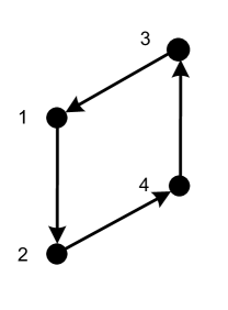
(b)

Figure 1: Examples of graphs: (a) a directed tree with root $4$; (b) a cyclic graph of period $4$

The “minimal” quasi-strongly connected graph is a directed tree (Fig. 1a), that is, a graph with only one root node, from where any other node is reachable via only one walk. A directed spanning tree in a graph $\mathcal{G}$ is a directed tree, contained by the graph $\mathcal{G}$ and including all of its nodes (Fig. 2b). It can be shown [56] that a graph has at least one directed spanning tree if and only if it is quasi-strongly connected. Nodes of a graph without directed spanning tree are covered by several directed trees, or spanning forest [58].

(a)

(b)

Figure 2: A quasi-strongly connected graph (a) and one of its directed spanning trees (b)

Definition 7

(Components) A strong subgraph $\mathcal{G}^{\prime}$ of the graph $\mathcal{G}$ is called a strongly connected (or strong) component, if it is not contained by any larger strong subgraph. A strong component that has no incoming arcs from other components is called closed.

Any node of a graph is contained in one and only one strong component. This component may correspond with the whole graph; this holds if and only if the graph is strong. If the graph is not strongly connected, then it contains two or more strong components, and at least one of them is closed. A graph is quasi-strongly connected if and only if this closed strong component is unique; in this case, any node of this strong component is a root node.

Definition 7 is illustrated by Fig. 3, showing two graphs with the same structure of strong components. The graph in Fig. 3a has the single root node $4$, constituting its own strong component, all other strong components are not closed. The graph in Fig. 3b has two closed strong components $\{4\}$ and $\{5,6,\ldots,10\}$.

(a)

(b)

Figure 3: Strong components of a rooted graph (a) and a graph without roots (b)

2.3 Nonnegative matrices and their graphs

In this subsection we discuss some results from matrix theory, regarding nonnegative matrices [59, 60, 61, 62].

Definition 8

(Irreducibility) A nonnegative matrix $A$ is irreducible if $\mathcal{G}[A]$ is strongly connected.

Theorem 1

(Perron-Frobenius) The spectral radius $\rho(A)\geq 0$ of a nonnegative matrix $A$ is an eigenvalue of $A$, for which a real nonnegative eigenvector exists

$$Av=\rho(A)v\;\;\text{for some}\;\;v=(v_{1},\ldots,v_{n})^{\top}\neq 0,\,v_{i}\geq 0.$$

If $A$ is irreducible, then $\rho(A)$ is a simple eigenvalue and $v$ is strictly positive $v_{i}>0\,\forall i$.

Obviously, Theorem 1 is also applicable to the transposed matrix $A^{\top}$, and thus $A$ also has a left nonnegative eigenvector $w^{\top}$, such that $w^{\top}A=\rho(A)w^{\top}$.

Besides $\rho(A)$, a nonnegative matrix can have other eigenvalues $\lambda$ of maximal modulus $|\lambda|=\rho(A)$. These eigenvalues have the following property [62, Ch.XIII].

Lemma 2

If $A$ is a nonnegative matrix and $\lambda\in\mathbb{C}$ is its eigenvalue with $|\lambda|=\rho(A)$, then the algebraic and geometric multiplicities of $\lambda$ coincide (that is, all Jordan blocks corresponding to $\lambda$ are trivial).

For an irreducible matrix, the eigenvalues of maximal modulus are always simple and have the form $\rho(A)e^{2\pi m\mathrm{\bf i}/h}$, where $h\geq 1$ is some integer and $m=0,1,\ldots,h-1$. This fundamental property is proved e.g. in [60, Sections 8.4 and 8.5] and [61, Section 8.3].

Theorem 3

Let an irreducible matrix $A$ have $h\geq 1$ different eigenvalues $\lambda_{1},\ldots,\lambda_{h}$ on the circle $\{\lambda\in\mathbb{C}:|\lambda|=\rho(A)\}$. Then, the following statements hold:

1. each $\lambda_{i}$ has the algebraic multiplicity $1$;

2. $\{\lambda_{1},\ldots,\lambda_{h}\}$ are roots of the equation $\lambda^{h}=r^{h}$;

3. if $h=1$ then all entries of the matrix $A^{k}$ are strictly positive when $k$ is sufficiently large;

4. if $h>1$, the matrix $A^{k}$ may have positive diagonal entries only when $k$ is a multiple of $h$.

Definition 9

(Primitivity) An irreducible nonnegative matrix $A$ is primitive if $h=1$, i.e. $\lambda=\rho(A)$ is the only eigenvalue of maximal modulus; otherwise, $A$ is called imprimitive or cyclic.

It can be shown via induction on $k=1,2,\ldots$ that if $A$ is a nonnegative matrix and $B=(b_{ij})=A^{k}$, then $b_{ij}>0$ if and only if in $\mathcal{G}[A]$ there exists a walk of length $k$ from $j$ to $i$. In particular, the diagonal entry $(A^{k})_{ii}$ is positive if and only if a cycle of length $k$ from node $i$ to itself exists. Hence, cyclic irreducible matrices correspond to periodic strong graphs.

Definition 10

(Periodicity) A graph is periodic if it has at least one cycle and the length of any cycle is divided by some integer $h>1$. The maximal $h$ with such a property is said to be the period of the graph. Otherwise, a graph is called aperiodic.

The simplest example of a periodic graph is a cyclic graph (Fig. 1b). Any graph with self-loops is aperiodic. Theorem 3 implies the following corollary.

Corollary 4

An irreducible matrix $A$ is primitive if and only if $\mathcal{G}[A]$ is aperiodic. Otherwise, $\mathcal{G}[A]$ is periodic with period $h$, where $h>1$ is the number of eigenvalues of the maximal modulus $\rho(A)$.

Many models of opinion dynamics employ stochastic and substochastic nonnegative matrices.

Definition 11

(Stochasticity and substochasticity) A nonnegative matrix $A$ (not necessarily square) is called stochastic if all its rows sum to $1$ (i.e. $\sum_{j}a_{ij}=1\,\forall i$) and substochastic if the sum of each row is no greater than $1$ (i.e. $\sum_{j}a_{ij}\leq 1\,\forall i$).

The Gershgorin Disc Theorem [60, Ch. 6] implies that $\rho(A)\leq 1$ for any square substochastic matrix $A$. If $A$ is stochastic then $\rho(A)=1$ since $A$ has an eigenvector of ones $\mathbbm{1}\stackrel{{\scriptstyle\Delta}}{{=}}(1,\ldots,1)^{\top}$: $A\mathbbm{1}=\mathbbm{1}$. A substochastic matrix $A$, as shown in [63], either is Schur stable or has a stochastic submatrix $A^{\prime}=(a_{ij})_{i,j\in V^{\prime}}$, where $V^{\prime}\subseteq\{1,\ldots,n\}$; an irreducible substochastic matrix is either stochastic or Schur stable [61, 63].

2.4 M-matrices and Laplacians of weighted graphs

In this subsection we introduce the class of M-matrices [59, 61] that are closely related to nonnegative matrices and have some important properties.

Definition 12

(M-matrix) A square matrix $Z$ is an M-matrix if it admits a decomposition $Z=sI-A$, where $s\geq\rho(A)$ and the matrix $A$ is nonnegative.

For instance, if $A$ is a substochastic matrix then $Z=I-A$ is an M-matrix. Another important class of M-matrices is given by the following lemma.

Lemma 5

Let $Z=(z_{ij})$ satisfies the following two conditions: 1) $z_{ij}\leq 0$ when $i\neq j$; 2) $z_{ii}\geq\sum_{j\neq i}|z_{ij}|$. Then, $Z$ is an M-matrix; precisely, $A=sI-Z$ is nonnegative and $\rho(A)\leq s$ whenever $s\geq\max_{i}z_{ii}$.

Indeed, if $s\geq\max_{i}z_{ii}$ then $A=sI-Z$ is nonnegative and $\rho(A)\leq\max_{i}(s-z_{ii}+\sum_{j\neq i}|z_{ij}|)\leq s$ thanks to the Gershgorin Disc Theorem [60].

Noticing that the eigenvalues of $Z$ and $A$ are in one-to-one correspondence $\lambda\mapsto s-\lambda$ and using Theorem 1 and Lemma 2, one arrives at the following result.

Corollary 6

Any M-matrix $Z=sI-A$ has a real eigenvalue $\lambda_{0}=s-\rho(A)\geq 0$, whose algebraic and geometric multiplicities coincide. For this eigenvalue there exist nonnegative right and left eigenvectors $v$ and $p$: $Zv=\lambda_{0}v$, $p^{\top}Z=\lambda_{0}p^{\top}$. These vectors are positive if the graph $\mathcal{G}[-Z]$ is strongly connected. For any other eigenvalue $\lambda$ one has $\mathop{\rm Re}\nolimits\lambda>\lambda_{0}$, and hence $Z$ is non-singular ($\det Z\neq 0$) if and only if $s>\rho(A)$.

Non-singular $M$-matrices are featured by the following important property [59, 61].

Lemma 7

Let $Z=sI-A$ be a non-singular $M$-matrix, i.e. $s>\rho(A)$. Then $Z^{-1}$ is nonnegative.

An example of a singular M-matrix is the Laplacian (or Kirchhoff) matrix of a weighted graph [64, 54, 65].

Definition 13

(Laplacian) Given a weighted graph $\mathcal{G}=(V,E,A)$, its Laplacian matrix is defined by

$$L[A]=(l_{ij})_{i,j\in V},\;\text{where}\;\;l_{ij}=\begin{cases}-a_{ij},&i\neq j\\ \sum\limits_{j\neq i}a_{ij},&i=j.\end{cases}$$ (1)

The Laplacian is an M-matrix due to Lemma 5. Obviously, $L[A]$ has the eigenvalue $\lambda_{0}=0$ since $L[A]\mathbbm{1}_{n}=0$, where $n$ is the dimension of $A$. The zero eigenvalue is simple if and only if the graph $\mathcal{G}[A]$ has a directed spanning tree (quasi-strongly connected).

Lemma 8

For an arbitrary nonnegative square matrix $A$ the following conditions are equivalent

1. $0$ is an algebraically simple eigenvalue of $L[A]$;

2. if $L[A]v=0,\,v\in\mathbb{R}^{n}$ then $v=c\mathbbm{1}_{n}$ for some $c\in\mathbb{R}$ (e.g. $0$ is a geometrically simple eigenvalue);

3. the graph $\mathcal{G}[A]$ is quasi-strongly connected.

The equivalence of statements 1 and 2 follows from Corollary 6. The equivalence of statements 2 and 3 was in fact proved in [34] and rediscovered in recent papers [66, 67]. A more general relation between the kernel’s dimension $\dim\ker L[A]=n-\mathop{\rm rank}\nolimits L[A]$ and the graph’s structure has been established in [58, 65].

3 The French-DeGroot Opinion Pooling

One of the first agent-based models of opinion formation was proposed by the social psychologist French in his influential paper [68], binding together SNA and systems theory. Along with its generalization, suggested by DeGroot [38] and called “iterative opinion pooling”, this model describes a simple procedure, enabling several rational agents to reach consensus [69, 70, 71]; it may also be considered as an algorithm of non-Bayesian learning [72, 73]. The original goal of French, however, was not to study consensus and learning mechanisms but rather to find a mathematical model for social power [68, 74, 75]. An individual’s social power in the group is his/her ability to control the group’s behavior, indicating thus the centrality of the individual’s node in the social network. French’s work has thus revealed a profound relation between opinion formation and centrality measures.

3.1 The French-DeGroot model of opinion formation

The French-DeGroot model describes a discrete-time process of opinion formation in a group of $n$ agents, whose opinions henceforth are denoted by $x_{1},\ldots,x_{n}$. First we consider the case of scalar opinions $x_{i}\in\mathbb{R}$. The key parameter of the model is a stochastic $n\times n$ matrix of influence weights $W=(w_{ij})$. The influence weights $w_{ij}\geq 0$, where $j=1,\ldots,n$ may be considered as some finite resource, distributed by agent $i$ to self and the other agents. Given a positive influence weight $w_{ij}>0$, agent $j$ is able to influence the opinion of agent $i$ at each step of the opinion iteration; the greater weight is assigned to agent $j$, the stronger is its influence on agent $i$. Mathematically, the vector of opinions $x(k)=(x_{1}(k),\ldots,x_{n}(k))^{\top}$ obeys the equation

$$x(k+1)=Wx(k),\quad k=0,1,\ldots.$$ (2)

which is equivalent to the system of equations

$$x_{i}(k+1)=\sum_{j=1}^{n}w_{ij}x_{j}(k),\,\forall i\quad k=0,1,\ldots.$$ (3)

Hence $w_{ij}$ is the contribution of agent $j$’s opinion at each step of the opinion iteration to the opinion of agent $i$ at its next step. The self-influence weight $w_{ii}\geq 0$ indicates the agent’s openness to the assimilation of the others’ opinions: the agent with $w_{ii}=0$ is open-minded and completely relies on the others’ opinions, whereas the agent with $w_{ii}=1$ (and $w_{ij}=0\,\forall j\neq i$) is a stubborn or zealot agent, “anchored” to its initial opinion $x_{i}(k)\equiv x_{i}(0)$.

More generally, agent’s opinions may be vectors of dimension $m$, conveniently represented by rows $x^{i}=(x_{i1},\ldots,x_{im})$. Stacking these rows on top of one another, one obtains an opinion matrix $X=(x_{il})\in\mathbb{R}^{n\times m}$. The equation (2) should be replaced by

$$X(k+1)=WX(k),\quad k=0,1,\ldots.$$ (4)

Every column $x_{i}(k)=(x_{1i}(k),\ldots,x_{ni}(k))^{\top}\in\mathbb{R}^{n}$ of $X(k)$, obviously, evolves in accordance with (2). Henceforth the model (4) with a general stochastic matrix $W$ is referred to as the French-DeGroot model.

3.2 History of the French-DeGroot model

A special case of the model (2) has been introduced by French in his seminal paper [68]. This paper first introduces a graph $\mathcal{G}$, whose nodes correspond to the agents; it is assumed that each node has a self-loop. An arc $(j,i)$ exists if agent $j$’s opinion is displayed to agent $i$, or $j$ “has power over” $i$. At each stage of the opinion iteration, an agent updates its opinion to the mean value of the opinions, displayed to it, e.g. the weighted graph in Fig. 4 corresponds to the dynamics

$$\begin{bmatrix}x_{1}(k+1)\\ x_{2}(k+1)\\ x_{3}(k+1)\end{bmatrix}=\begin{pmatrix}1/2&1/2&0\\ 1/3&1/3&1/3\\ 0&1/2&1/2\end{pmatrix}\begin{bmatrix}x_{1}(k)\\ x_{2}(k)\\ x_{3}(k)\end{bmatrix}.$$ (5)

Obviously, the French’s model is a special case of equation (2), where the matrix $W$ is adapted to the graph $\mathcal{G}$ and has positive diagonal entries; furthermore, in each row of $W$ all non-zero entries are equal. Hence each agent uniformly distributes influence between itself and the other nodes connected to it.

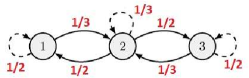
Figure 4: An example of the French model with $n=3$ agents

French formulated without proofs several conditions for reaching a consensus, i.e. the convergence $x_{i}(k)\xrightarrow[k\to\infty]{}x_{*}$ of all opinions to a common “unanimous opinion” [68] that were later corrected and rigorously proved by Harary [76, 53]. His primary interest was, however, to find a quantitative characteristics of the agent’s social power, that is, its ability to influence the group’s collective opinion $x_{*}$ (the formal definition will be given in Subsect. 3.5).

A general model (4), proposed by DeGroot [38], takes its origin in applied statistics and has been suggested as a heuristic procedure to find “consensus of subjective probabilities” [77]. Each of $n$ agents (“experts”) has a vector opinion, standing for an individual (“subjective”) probability distribution of $m$ outcomes in some random experiment; the experts’ goal is to “form a distribution which represents, in some sense, a consensus of individual distributions” [77]. This distribution was defined in [77] as the unique Nash equilibrium [78] in a special non-cooperative “Pari-Mutuel” game (betting on horse races), which can be found by solving a special optimization problem, referred now to as the Eisenberg-Gale convex program [79]. To obtain a simpler algorithm of reaching consensus, a heuristical algorithm was suggested in [80], replacing the convex optimization by a very simple procedure of weighted averaging, or opinion pooling [81]. Developing this approach, the procedure of iterative opinion pooling (4) was suggested in [38]. Unlike [77, 80], the DeGroot procedure was a decentralized algorithm: each agent modifies its opinion independently based on the opinions of several “trusted” individuals, and there may be no agent aware of the opinions of the whole group. Unlike the French model [68], the matrix $W$ can be an arbitrary stochastic matrix and the opinions are vector-valued.

3.3 Algebraic convergence criteria

In this subsection, we discuss convergence properties of the French-DeGroot model (2); the properties for the multidimensional model (4) are the same.

A straightforward computation shows that the dynamics (2) is “non-expansive” in the sense that

$$\begin{gathered}\min_{i}x_{i}(0)\leq\cdots\leq\min_{i}x_{i}(k)\leq\min_{i}x_{i}(k+1),\\ \max_{i}x_{i}(0)\geq\cdots\geq\max_{i}x_{i}(k)\geq\max_{i}x_{i}(k+1)\\ \end{gathered}$$

for any $k=0,1,\ldots$. In particular, the system (2) is always Lyapunov stable, but this stability is not asymptotic since $W$ always has eigenvalue at $1$.

The first question, regarding the model (4), is whether the opinions converge or oscillate. A more specific problem is convergence to a consensus [38].

Definition 14

(Convergence) The model (2) is convergent if for any initial condition $x(0)$ the limit exists

$$x(\infty)=\lim_{k\to\infty}x(k)=\lim_{k\to\infty}W^{k}x(0).$$ (6)

A convergent model reaches a consensus if $x_{1}(\infty)=\ldots=x_{n}(\infty)$ for any initial opinion vector $x(0)$.

The convergence and consensus in the model (2) are equivalent, respectively, to regularity and full regularity of the stochastic matrix $W$.

Definition 15

(Regularity) We call the matrix $W$ regular if the limit $W^{\infty}=\lim\limits_{k\to\infty}W^{k}$ exists and fully regular if, additionally, the rows of $W^{\infty}$ are identical (that is, $W^{\infty}=\mathbbm{1}_{n}p^{\top}_{\infty}$ for some $p_{\infty}\in\mathbb{R}^{n}$).

Lemma 2 entails the following convergence criterion.

Lemma 9

[62, Ch.XIII] The model (2) is convergent (i.e. $W$ is regular) if and only if $\lambda=1$ is the only eigenvalue of $W$ on the unit circle $\{\lambda\in\mathbb{C}:|\lambda|=1\}$. The model (2) reaches consensus (i.e. $W$ is fully regular) if and only if this eigenvalue is simple, i.e. the corresponding eigenspace is spanned by the vector $\mathbbm{1}$.

Using Theorem 3, Lemma 9 implies the equivalence of convergence and consensus when $W$ is irreducible.

Lemma 10

For an irreducible stochastic matrix $W$ the model (2) is convergent if and only if $W$ is primitive, i.e. $W^{k}$ is a positive matrix for large $k$. In this case consensus is also reached.

Since an imprimitive irreducible matrix $W$ has eigenvalues $\{e^{2\pi k\mathrm{\bf i}/h}\}_{k=0}^{h-1}$, where $h>1$, for almost all initial conditions the solution of (2) oscillates.

3.4 Graph-theoretic conditions for convergence

For large-scale social networks, the criterion from Lemma 9 cannot be easily tested. In fact, convergence of the French-DeGroot model (2) does not depend on the weights $w_{ij}$ , but only on the graph $\mathcal{G}[W]$. In this subsection, we discuss graph-theoretic conditions for convergence and consensus. Using Corollary 4, Lemma 10 may be reformulated as follows.

Lemma 11

If the graph $\mathcal{G}=\mathcal{G}[W]$ is strong, then the model (2) reaches a consensus if and only if $\mathcal{G}$ is aperiodic. Otherwise, the model is not convergent and opinions oscillate for almost all $x(0)$.

Considering the general situation, where $\mathcal{G}[W]$ has more than one strong component, one may easily notice that the evolution of the opinions in any closed strong component is independent from the remaining network. Two different closed components obviously cannot reach consensus for a general initial condition.

This implies that for convergence of the opinions it is necessary that all closed strong components are aperiodic. For reaching a consensus the graph $\mathcal{G}[W]$ should have the only closed strong component (i.e. be quasi-strongly connected), which is aperiodic. Both conditions, in fact, appear to be sufficient.

Theorem 12

[86, 10] The model (2) is convergent if and only if all closed strong components in $\mathcal{G}[W]$ are aperiodic. The model (2) reaches a consensus if and only if $\mathcal{G}[W]$ is quasi-strongly connected and the only closed strong component is aperiodic.

As shown in the next subsection, Theorem 12 can be derived from the standard results on the Markov chains convergence [82], using the duality between Markov chains and the French-DeGroot opinion dynamics. Theorem 12 has an important corollary, used in the literature on multi-agent consensus.

Corollary 13

Let the agents’ self-weights be positive $w_{ii}>0\,\forall i$. Then, the model (2) is convergent. It reaches a consensus if and only if $\mathcal{G}[W]$ is quasi-strongly connected (i.e. has a directed spanning tree).

It should be noted that the existence of a directed spanning tree is in general not sufficient for consensus in the case where $W$ has zero diagonal entries. The second part of Corollary 13 was proved in [76] and included, without proof, in [53, Chapter 4]. Numerous extensions of this result to time-varying matrices $W(k)$ [87, 86, 88, 56, 89] and more general nonlinear consensus algorithms [90, 91] have recently been obtained. Some time-varying extensions of the French-DeGroot model, namely, bounded confidence opinion dynamics [92] and dynamics of reflected appraisal [93] will be discussed in Part II of this tutorial.

3.5 The dual Markov chain and social power

Notice that the matrix $W$ may be considered as a matrix of transition probabilities of some Markov chain with $n$ states. Denoting by $p_{i}(t)$ the probability of being at state $i$ at time $t$, the row vector $p^{\top}(t)=(p_{1}(t),\ldots,p_{n}(t))$ obeys the equation

$$p(k+1)^{\top}=p(k)^{\top}W,\quad t=0,1,\ldots$$ (7)

The convergence of (2), that is, regularity of $W$ implies that the probability distribution converges to the limit $p(\infty)^{\top}=\lim_{k\to\infty}p(k)^{\top}=p(0)^{\top}W^{\infty}$. Consensus in (2) implies that $p(\infty)=p_{\infty}$, where $p_{\infty}$ is the vector from Definition 15, i.e. the Markov chain “forgets” its history and convergence to the unique stationary distribution. Such a chain is called regular or ergodic [94, 62]. The closed strong components in $\mathcal{G}[W]$ correspond to essential classes of states, whereas the remaining nodes correspond to inessential (or non-recurrent) states [94]. The standard ergodicity condition is that the essential class is unique and aperiodic, which is in fact equivalent to the second part of Theorem 12. The first part of Theorem 12 states another known fact [94]: the Markov chain always converges to a stationary distribution if and only if all essential classes are aperiodic.

Assuming that $W$ is fully regular, one notices that

$$x(k+1)=W^{k}x(0)\xrightarrow[k\to\infty]{}(p_{\infty}^{\top}x(0))\mathbbm{1}_{n}.$$ (8)

The element $p_{\infty i}$ can thus be treated as a measure of social power of agent $i$, i.e. the weight of its initial opinion $x_{i}(0)$ in the final opinion of the group. The greater this weight is, the more influential is the $i$th individual’s opinion. A more detailed discussion of social power and social influence mechanism is provided in [68, 75]. The social power may be considered as a centrality measure, allowing to identify the most “important” (influential) nodes of a social network. This centrality measure is similar to the eigenvector centrality [95], which is defined as the left eigenvector of the conventional binary adjacency matrix of a graph instead of the “normalized” stochastic adjacency matrix. Usually centrality measures are introduced as functions of the graph topology [96] while their relations to dynamical processes over graphs are not well studied. French’s model of social power introduces a dynamic mechanism of centrality measure and a decentralized algorithm (7) to compute it.

Example 1

Consider the French model with $n=3$ agents (5), corresponding to the graph in Fig. 4. One can expect that the “central” node $2$ corresponds to the most influential agent in the group. This is confirmed by a straightforward computation: solving the system of equations $p_{\infty}^{\top}=p_{\infty}^{\top}W$ and $p_{\infty}^{\top}\mathbbm{1}=1$, one obtains the vector of social powers $p_{\infty}^{\top}=(\tfrac{2}{7},\tfrac{3}{7},\tfrac{2}{7})$.

3.6 Stubborn agents in the French-DeGroot model

Although consensus is a typical behavior of the model (2), there are situations when the opinions do not reach consensus but split into several clusters. One of the reasons for that is the presence of stubborn agents (called also radicals [97] or zealots [98]).

Definition 16

(Stubbornness) An agent is said to be stubborn if its opinion remains unchanged independent of the others’ opinions.

If the opinions obey the model (2) then agent $i$ is stubborn $x_{i}(k)\equiv x_{i}(0)$ if and only if $w_{ii}=1$. Such an agent corresponds to a source node in a graph $\mathcal{G}[W]$, i.e. a node having no incoming arcs but for the self-loop (Fig. 5).

Figure 5: The graph of the French-DeGroot model with two stubborn agents (source nodes) 1 and 3.

Theorem 12 implies that if $\mathcal{G}[W]$ has the only source, being also a root (Fig. 3a), then the opinions reach a consensus (the source node is the only closed strong component of the graph). If more than one stubborn agent exist (i.e. $\mathcal{G}[W]$ has several sources), then consensus among them is, obviously, impossible. Theorem 12 implies, however, that typically the opinions in such a group converge.

Corollary 14

Let the group have $s\geq 1$ stubborn agents, influencing all other individuals (i.e. the set of source nodes is connected by walks to all other nodes of $\mathcal{G}[W]$). Then the model (2) is convergent.

Indeed, source nodes are the only closed strong components of $\mathcal{G}[W]$, which are obviously aperiodic.

In Section 6 it will be shown that under the assumptions of Corollary 14 the final opinion $x(\infty)$ is fully determined by the stubborn agents’ opinions.

Example 2

Consider the French-DeGroot model, corresponding to the weighted graph in Fig. 5

$$\begin{bmatrix}x_{1}(k+1)\\ x_{2}(k+1)\\ x_{3}(k+1)\end{bmatrix}=\begin{pmatrix}1&0&0\\ \frac{1}{3}&\frac{1}{3}&\frac{1}{3}\\ 0&0&1\end{pmatrix}\begin{bmatrix}x_{1}(k)\\ x_{2}(k)\\ x_{3}(k)\end{bmatrix}.$$

It can be shown that the steady opinion vector of this model is $x(\infty)=(x_{1}(0),x_{1}(0)/2+x_{3}(0)/2,x_{3}(0))^{\top}$.

4 Abelson’s Models and Diversity Puzzle

In his influential work [34] Abelson proposed a continuous-time counterpart of the French-DeGroot model (2). Besides this model and its nonlinear extensions, he formulated a key problem in opinion formation modeling, referred to as the community cleavage problem [19] or Abelson’s diversity puzzle [99].

4.1 Abelson’s models of opinion dynamics

To introduce Abelson’s model, we first consider an alternative interpretation of the French-DeGroot model (2). Recalling that $1-w_{ii}=\sum_{j\neq i}w_{ij}$, one has

$$\underbrace{x_{i}(k+1)-x_{i}(k)}_{\Delta x_{i}(k)}=\sum_{j\neq i}\underbrace{w_{ij}[x_{j}(k)-x_{i}(k)]}_{\Delta_{(j)}x_{i}(k)}\quad\forall i.$$ (9)

The experiments with dyadic interactions ($n=2$) show that “the attitude positions of two discussants … move toward each other” [52]. The equation (9) stipulates that this argument holds for simultaneous interactions of multiple agents: adjusting its opinion $x_{i}(k)$ by $\Delta_{(j)}x_{i}(k)$, agent $i$ shifts it towards $x_{j}(k)$ as

$$x_{i}^{\prime}=x_{i}+\Delta_{(j)}x_{i}\Longrightarrow|x_{j}-x_{i}^{\prime}|=(1-w_{ij})|x_{j}-x_{i}|.$$

The increment in the $i$th agent’s opinion $\Delta x_{i}(k)$ is the “resultant” of these simultaneous adjustments.

Supposing that the time elapsed between two steps of the opinion iteration is very small, the model (9) can be replaced by the continuous-time dynamics

$$\dot{x}_{i}(t)=\sum_{j\neq i}a_{ij}(x_{j}(t)-x_{i}(t)),\,i=1,\ldots,n.$$ (10)

Here $A=(a_{ij})$ is a non-negative (but not necessarily stochastic) matrix of infinitesimal influence weights (or “contact rates” [34, 52]). The infinitesimal shift of the $i$th opinion $dx_{i}(t)=\dot{x}_{i}(t)dt$ is the superposition of the infinitesimal’s shifts $a_{ij}(x_{j}(t)-x_{i}(t))dt$ of agent $i$’s towards the influencers. A more general nonlinear mechanism of opinion evolution [34, 52, 35] is

$$\dot{x}_{i}(t)=\sum_{j\neq i}a_{ij}g(x_{i},x_{j})(x_{j}(t)-x_{i}(t))\,\quad\forall i.$$ (11)

Here $g:\mathbb{R}\times\mathbb{R}\to(0;1]$ is a coupling function, describing the complex mechanism of opinion assimilation.

In this section, we mainly deal with the linear Abelson model (10), whose equivalent matrix form is

$$\dot{x}(t)=-L[A]x(t),$$ (12)

where $L[A]$ is the Laplacian matrix (1). Recently the dynamics (12) has been rediscovered in multi-agent control theory [100, 56, 101] as a continuous-time consensus algorithm. We discuss the convergence properties of this model in the next subsection.

4.2 Convergence and consensus conditions

Note that Corollary 6, applied to the M-matrix $L[A]$ and $\lambda_{0}=0$, implies that all Jordan blocks, corresponding to the eigenvalue $\lambda_{0}=0$, are trivial and for any other eigenvalue $\lambda$ of the Laplacian $L[A]$ one has $\mathop{\rm Re}\nolimits\lambda>0$. Thus, the model (12) is Lyapunov stable (yet not asymptotically stable) and, unlike the French-DeGroot model, is always convergent.

Corollary 15

For any nonnegative matrix $A$ the limit $P^{\infty}=\lim\limits_{t\to\infty}e^{-L[A]t}$ exists, and thus the vector of opinions in (12) converges $x(t)\xrightarrow[t\to\infty]{}x^{\infty}=P^{\infty}x(0)$.

The matrix $P^{\infty}$ is a projection operator onto the Laplacian’s null space $\ker L[A]=\{v:L[A]v=0\}$ and is closely related to the graph’s structure [58, 102].

Similar to the discrete-time model (2), the system (12) reaches a consensus if the final opinions coincide $x^{\infty}_{1}=\ldots=x^{\infty}_{n}$ for any initial condition $x(0)$. Obviously, consensus means that $\ker L[A]$ is spanned by the vector $\mathbbm{1}_{n}$, i.e. $P^{\infty}=\mathbbm{1}_{n}p^{\top}_{\infty}$, where $p\in\mathbb{R}^{n}$ is some vector. By noticing that $x=\mathbbm{1}_{n}$ is an equilibrium point, one has $P\mathbbm{1}_{n}=\mathbbm{1}_{n}$ and thus $p^{\top}_{\infty}\mathbbm{1}_{n}=1$. Since $P$ commutes with $L[A]$, it can be easily shown that $p^{\top}_{\infty}L[A]=0$. Recalling that $L[A]$ has a nonnegative left eigenvector $p$ such that $p^{\top}L[A]=0$ due to Corollary 6 and $\dim\ker L[A]=1$, one has $p_{\infty}=cp$, where $c>0$. Combining this with Lemma 8, one obtains the following consensus criterion.

Theorem 16

The linear Abelson model (12) reaches consensus if and only if $\mathcal{G}[A]$ is quasi-strongly connected (i.e. has a directed spanning tree). In this case, the opinions converge to the limit

$$\lim_{t\to\infty}x_{1}(t)=\ldots=\lim_{t\to\infty}x_{n}(t)=p_{\infty}^{\top}x(0),$$

where $p_{\infty}\in\mathbb{R}^{n}$ is the nonnegative vector, uniquely defined by the equations $p_{\infty}^{\top}L[A]=0$ and $p^{\top}_{\infty}\mathbbm{1}_{n}=1$.

Similar to the French-DeGroot model, the vector $p_{\infty}$ may be treated as a vector of the agents’ social powers, or a centrality measure on the nodes of $\mathcal{G}[A]$.

It is remarkable that a crucial part of Theorem 16 was proved by Abelson [34], who called quasi-strongly connected graphs “compact”. Abelson proved that the null space $\ker L[A]$ consists of the vectors $c\mathbbm{1}_{n}$ if and only if the graph is “compact”, i.e. statements 2 and 3 in Lemma 8 are equivalent. He concluded that “compactness” is necessary and sufficient for consensus; the proof, however, was given only for diagonalizable Laplacian matrices. In general, the sufficiency part requires to prove that the zero eigenvalue of $L[A]$ is algebraically simple (statement 1 in Lemma 8). The full proof of Theorem 16 was given only in [66]; the case of strong graph was earlier considered in [100].

As already discussed, the model (12) arises as a “limit” of the French-DeGroot model as the time between consecutive opinion updates becomes negligibly small. The inverse operation of discretization transforms (12) into the French-DeGroot model.

Lemma 17

[66, 56] For any nonnegative matrix $A$ and $\tau>0$ the matrix $W_{\tau}=e^{-\tau L[A]}$ is stochastic, and thus $P^{\infty}=\lim\limits_{\tau\to\infty}W_{\tau}$ from Corollary 15 is stochastic. The matrices $W_{\tau}$ have positive diagonal entries.

Lemma 17 implies that the vectors $\tilde{x}(k)=x(\tau k)$ satisfy a special French-DeGroot model with $W=W_{\tau}$ and allows to derive Theorem 16 from Corollary 13; this lemma can also be used for analysis of time-varying extensions of Abelson’s model [56].

Many results, regarding consensus algorithms over time-varying graphs, have been obtained in [100, 56, 101, 103, 104, 105, 106, 107, 108] and extended to general dynamic agents [56, 57, 109, 110, 111]. More advanced results on nonlinear consensus algorithms [112, 105, 113] allow to examine the nonlinear Abelson model (11) under different assumptions on the coupling function $g(\cdot)$. The statement of Abelson [34, 52] that the model (11) reaches consensus for any function $g(a,b)\in(0;1]$ when $\mathcal{G}[A]$ is “compact” (quasi-strongly connected) is, obviously, incorrect unless additional assumptions are adopted; however, it holds for continuous function $g(a,b)$, as implied by the results of [112, 113].

4.3 The community cleavage problem

Admitting that in general the outcome of consensus is “too strong to be realistic” [52], Abelson formulated a fundamental problem, called the community cleavage problem [19] or Abelson’s diversity puzzle [99]. The informal formulation, stated in [34], was: “Since universal ultimate agreement is an ubiquitous outcome of a very broad class of mathematical models, we are naturally led to inquire what on earth one must assume in order to generate the bimodal outcome of community cleavage studies.” In other words, the reasons for social cleavage, that is, persistent disagreement among the agents’ opinions (e.g. clustering [114]) are to be identified. This requires to find mathematical models of opinion formation that are able to capture the complex behavior of real social groups, yet simple enough to be rigorously examined.

As discussed in Subsect. 3.6, one of the reasons for opinion clustering is the presence of stubborn agents, whose opinions are invariant. In the models (10) and (11), agent $i$ is stubborn if and only if $a_{ij}=0\,\forall j$, corresponding thus to a source node of the graph $\mathcal{G}[A]$. In the next sections we consider more general models with “partially” stubborn, or prejudiced, agents.

5 Cleavage and Prejudices: Taylor’s model

In this section, we consider an extension of the linear Abelson model (10), proposed in [115]. Whereas the French-DeGroot and Abelson models have triggered extensive studies on multi-agent consensus, Taylor’s model in fact has anticipated the recent studies on containment control algorithms [116, 57, 117, 118].

The model from [115], as usual, involves $n$ agents with opinions $x_{1},\ldots,x_{n}\in\mathbb{R}$ and $m\geq 1$ communication sources (such as e.g. mass media), providing static opinions $s_{1},\ldots,s_{m}\in\mathbb{R}$. The agents’ opinions are influenced by these sources, obeying the model

$$\dot{x}_{i}(t)=\sum_{j=1}^{n}a_{ij}(x_{j}(t)-x_{i}(t))+\sum_{k=1}^{m}b_{ik}(s_{k}-x_{i}(t)).$$ (13)

Besides the nonnegative matrix of influence weights $A=(a_{ij})$, the Taylor model (13) involves the non-square $n\times m$ nonnegative matrix $B=(b_{ik})$ of “persuasibility constants” [115], which describe the influence of the communication sources on the agents. Some agents can be free of the external influence $b_{i1}=\ldots=b_{im}=0$, whereas the agents with $\sum_{k=1}^{m}b_{ik}>0$ are influenced by one or several sources. Taylor has shown that the presence of external influence typically causes the cleavage of opinions; moreover, unlike the Abelson model, the system (13) is usually asymptotically stable and converges to the unique equilibrium, determined by $s_{1},\ldots,s_{k}$.

Besides the linear model (13), Taylor [115] considered nonlinear opinion dynamics, which extend (11) and some other models from [34] and are still waiting for a rigorous mathematical examination. These systems are however beyond the scope of this tutorial.

5.1 Equivalent representations of the Taylor model

Note that formally the model (13) may be considered as the Abelson model with $n+k$ agents, where the “virtual” agents $n+1,\ldots,n+k$ are stubborn: $x_{n+i}=s_{i}$ for $i=1,\ldots,k$. Corollary 15 implies that the model (13) is convergent: for any $x(0)$ and $s_{1},\ldots,s_{k}$ there exist the limit $x(\infty)=\lim\limits_{t\to\infty}x(t)$. The converse is also true: for the Abelson model with $k\geq 1$ stubborn agents, their static opinions may be considered as “communication sources” for the others. However, some properties of the system (e.g. stability) are easier to formulate for Taylor’s system (13) than for the augmented Abelson’s model.

Another transformation allows to reduce (13) to a formally less general model, where each agent may have its own “communication source” or prejudice

$$\dot{x}_{i}(t)=\sum_{j=1}^{n}a_{ij}(x_{j}(t)-x_{i}(t))+\gamma_{i}(u_{i}-x_{i}(t))$$ (14)

where $\gamma_{i}\geq 0$. Obviously, (13) reduces to (14), choosing $\gamma_{i}\stackrel{{\scriptstyle\Delta}}{{=}}\sum_{m=1}^{k}b_{im}\geq 0$ and $u_{i}\stackrel{{\scriptstyle\Delta}}{{=}}\gamma_{i}^{-1}\sum_{m=1}^{k}b_{im}s_{m}$ (if $\gamma_{i}=0$, we set $u_{i}=0$ without loss of generality).

Definition 17

(Prejudiced agents) Given a group of $n$ agents, governed by the model (14), we call agent $i$ prejudiced if $\gamma_{i}>0$; the external inputs $u_{i}$ are referred to as the prejudices of corresponding agents.

The prejudice may be considered as some “internal” agent’s opinion, formed by some external factors (as in the Taylor model (13)) or the individual’s personal experience. An agent that is not prejudiced obeys the usual Abelson mechanism (10). A prejudiced agent may be totally closed to the interpersonal influence $a_{ij}=0\,\forall j$; in this case its opinion converges to its prejudice $x_{i}(t)\xrightarrow[t\to\infty]{}u_{i}$ and $\gamma_{i}$ regulates the convergence rate. In the special case where $u_{i}=x_{i}(0)$ such an agent is stubborn since $x_{i}(t)\equiv u_{i}$. The concept of a prejudiced agent is however much more general and allows the agent to be influenced by both its prejudice and the others’ opinions.

5.2 Stability of the Taylor model

In this subsection, we examine asymptotic stability of the Taylor model. Obviously, it suffices to examine only the system (14), to which the original model (13) reduces. Introducing the matrix $\Gamma=\mathop{\rm diag}\nolimits(\gamma_{1},\ldots,\gamma_{n})$, the model (14) is rewritten as

$$\dot{x}(t)=-(L[A]+\Gamma)x(t)+\Gamma u.$$ (15)

To examine the stability properties of (15), we split the agents into two classes. Agent $i$ is said to be P-dependent (prejudice-dependent) if is either prejudiced or influenced by some prejudiced agent $j$ (that is, a walk from $j$ to $i$ exists in the graph $\mathcal{G}[A]$). Otherwise, we call the agent P-independent. Renumbering the agents, we assume that agents $1,\ldots,r\geq 1$ are P-dependent and agents $r+1,\ldots,n$ are P-independent (possibly, $r=n$). Denote the corresponding parts of the opinion vector by, respectively, $x^{1}(t)$ and $x^{2}(t)$. Since P-dependent agents are not connected to P-independent ones, Eq. (15) is decomposed as follows

$$\dot{x}^{1}(t) =-(L^{11}+\Gamma^{11})x^{1}(t)-L^{12}x^{2}(t)+\Gamma^{11}u^{1}$$ (16)

$$\dot{x}^{2}(t) =-L^{22}x^{2}(t).$$ (17)

The matrix $L^{22}$ is Laplacian of size $(n-r)\times(n-r)$, i.e. (17) is the Abelson model. The matrix $L^{11}$ is, in general, not Laplacian; one has $L^{11}\mathbbm{1}_{r}\geq 0$.

Theorem 18

Let the community have $r\geq 1$ P-dependent agents and $n-r\geq 0$ P-independent ones. Then the dynamics of P-dependent agents (16) is asymptotically stable, i.e. the matrix $-(L^{11}+\Gamma^{11})$ is Hurwitz. The vector of their opinions converges to

$$x^{1}(\infty)=M\begin{bmatrix}u^{1}\\ x^{2}(\infty)\end{bmatrix},\;M\stackrel{{\scriptstyle\Delta}}{{=}}(L^{11}+\Gamma^{11})^{-1}\begin{bmatrix}\Gamma^{11}\quad L^{12}\end{bmatrix}.$$ (18)

The matrix $M$ is stochastic, and thus the final opinion of any agent is a convex combination of the prejudices and the final opinions of P-independent agents.

Theorem 18 easily follows from the properties of M-matrices. Using Lemma 5, $L^{11}+\Gamma^{11}$ is proved to be M-matrix. It suffices to show that the corresponding eigenvalue $\lambda_{0}$ from Corollary 6 is positive. Suppose on the contrary that $\lambda_{0}=0$ and let $p$ stand for the nonnegative left eigenvector $p^{\top}(L^{11}+\Gamma^{11})=0$. Multiplying by $\mathbbm{1}_{r}$ and noticing that $L^{11}\mathbbm{1}_{r}\geq 0$, one has $p^{\top}\Gamma^{11}\mathbbm{1}_{r}=0$, that is, $p^{\top}\Gamma^{11}=0$ and $p_{i}=0$ whenever $\gamma_{i}>0$, i.e. $p_{i}=0$ for all prejudiced agents $i$. Since $p^{\top}L^{11}=0$, for any $j$ such that $p_{j}=0$ one has $\sum_{i\neq j}p_{i}a_{ij}=p_{j}\sum_{j\neq i}a_{ji}=0$, i.e. $p_{i}=0$ whenever $a_{ij}>0$. In other words, if node $j$ is connected to node $i$ and $p_{j}=0$ then also $p_{i}=0$. This implies that $p=0$ which contradicts to the choice of $p$. This contradiction shows that $\lambda_{0}>0$ and hence the system (16) is stable, entailing (18). Since $(-L^{12})$ is nonnegative, Lemma 7 implies that the matrix $M$ is also nonnegative. Choosing $u=\mathbbm{1}_{n}$, it is obvious that (14) has an equilibrium $x=\mathbbm{1}_{n}$, which implies that $M\mathbbm{1}_{n}=\mathbbm{1}_{r}$, i.e. $M$ is stochastic, which ends the proof.

Corollary 19

The system (14) is asymptotically stable, i.e. the matrix $-(L[A]+\Gamma)$ is Hurwitz if and only if all agents are P-dependent.

In terms of the original model (13), Corollary 19 can be reformulated as follows: the system (13) is asymptotically stable if and only if any agent is influenced by at least one “communication source”. This influence can be direct (if $\gamma_{i}=\sum_{m=1}^{k}b_{im}>0$) or indirect (through a chain of the other agents).

5.3 The Taylor model and containment control

A multidimensional extension of the Taylor model (13) arises in the containment control problems [116, 57, 117, 118]. The agents stand for mobile robots or vehicles, and the “opinion” $x_{i}\in\mathbb{R}^{d}$ is the position of agent $i$. The “communication sources” $s_{1},\ldots,s_{k}\in\mathbb{R}^{d}$ are the positions of $k$ static leaders. The mobile agents’ goal is to reach the convex hull

$$\mathcal{S}\stackrel{{\scriptstyle\Delta}}{{=}}\left\{\sum_{m=1}^{k}\alpha_{m}s_{m}:\alpha_{m}\geq 0,\sum_{m=1}^{k}\alpha_{m}=1\right\}\subset\mathbb{R}^{d}$$

spanned by the leaders $s_{1},\ldots,s_{k}$. Agent $i$ is directly influenced by the leader $m$ (i.e. $b_{im}>0$) if it can measure its position (in general, none of the agents can observe the whole set $\mathcal{S}$). Similar to the scalar case, such agents can be called “prejudiced”. The other agents can be either “P-dependent” (indirectly influenced by one or several leaders) or “P-independent”.

Theorem 20

The three conditions are equivalent

1. the system (13) is Hurwitz stable;

2. any agent is influenced directly or indirectly by one of the leaders (P-dependent);

3. the mobile agents reach the target convex hull

   $$x_{i}(\infty)\in\mathcal{S}\quad\forall i=1,\ldots,n$$ (19)

   for any positions of the leaders $s_{1},\ldots,s_{k}\in\mathbb{R}^{d}$ and the initial conditions $x_{1}(0),\ldots,x_{n}(0)\in\mathbb{R}^{d}$.

The equivalence $1\Longleftrightarrow 2$ is established by Theorem 18. Obviously, $3\Longrightarrow 1$: choosing $s_{1}=\ldots=s_{k}=0$, one has $\mathcal{S}=\{0\}$ and (19) is the asymptotic stability condition. It remains to prove the implication $1\Longrightarrow 3$. In the scalar case $d=1$ it is immediate from Theorem 18. In general, let $v\in\mathbb{R}^{d}$ and $\tilde{x}_{i}(t)=v^{\top}x_{i}(t)$, $\tilde{s}_{m}=v^{\top}s_{m}$. Then, obviously $\tilde{x}_{i},\tilde{s}_{m}$ obey the scalar model (13) and thus $v^{\top}x_{i}(\infty)=\tilde{x}_{i}(\infty)\geq\min_{m}\tilde{s}_{m}=\min_{m}v^{\top}s_{m}=\min_{s\in\mathcal{S}}v^{\top}s$. Since $v$ is arbitrary, one has $x_{i}(\infty)\in\mathcal{S}$ for any $i$.

In the recent literature on containment control [116, 57, 117, 119, 120] Theorem 20 has been extended in various directions: the leaders may be dynamic (and thus their convex hull is time-varying $\mathcal{S}=\mathcal{S}(t)$), the interaction graph may also be time-varying and the agents may have non-trivial dynamics. Furthermore, the polyhedron $\mathcal{S}$ can be replaced by an arbitrary closed convex set; the relevant problem is sometimes referred to as the target aggregation [121] and is closely related to distributed optimization [122].

6 Friedkin-Johnsen Model

It is a remarkable fact that no discrete-time counterpart of the Taylor model had been suggested till 1990s, when Friedkin and Johnsen [123, 124, 125] introduced a discrete-time modification of the dynamics (14). Unlike many models of opinion formation, proposed in the literature, this model has been experimentally validated for small and medium-size groups, as reported in [125, 126, 127, 19, 93].

Similar to DeGroot’s dynamics (2), the Friedkin-Johnsen model employs a stochastic matrix of social influences $W$, corresponding to the influence graph $\mathcal{G}[W]$. Besides this matrix, a diagonal matrix $\Lambda=\mathop{\rm diag}\nolimits(\lambda_{1},\ldots,\lambda_{n})$ is introduced, where $\lambda_{i}\in[0,1]$ stands for the susceptibility of agent $i$ to the process of social influence. The vector of the agents’ opinions evolves in accordance with

$$x(k+1)=\Lambda Wx(k)+(I-\Lambda)u.$$ (20)

Here $u$ is a constant vector of the agents’ prejudices. The susceptibilities’ complements $1-\lambda_{i}$ play the same role as the coefficients $\gamma_{i}$ in (14); in the case $\Lambda=0$ the model (20) turns into the French-DeGroot model (2). If $1-\lambda_{i}=0$ then agent $i$ is independent of the prejudice vector $u$ and applies the usual French-DeGroot “opinion pooling” rule. When $\lambda_{i}<1$, agent $i$ is “anchored” to its prejudice $u_{i}$ and factors its into any opinion iteration. If $\lambda_{i}=0$ then the $i$th agent’s opinion stabilizes at the first step $x_{i}(k)\equiv u_{i}\,\forall k\geq 1$; such an agent is stubborn $x_{i}(k)\equiv x_{i}(0)$ when $u_{i}=x_{i}(0)$.

In the Friedkin-Johnsen theory [125, 127, 19] it is supposed traditionally that $u=x(0)$, i.e. the prejudices of the agents are their initial opinions. This is explained by the assumption [125] that the individuals prejudices have been formed by some exogenous conditions, which influenced the group in the past; in this sense the vectors of prejudices $u$ and initial opinions $x(0)$ store the information about the group’s history. The assumption $u=x(0)$ in turn motivates to adopt the “coupling condition” $1-\lambda_{i}=w_{ii}$, stating that the levels of agents’ “anchorage” to the initial opinions are determined by their self-confidence weights. At the same time, similar to Taylor’s model, the prejudice may be independent of the initial opinion $x(0)$ and caused by media or some other “communication sources”. For this reason, we do not adopt these coupling conditions in this tutorial, allowing the prejudices and initial opinions to be independent; the same holds for the matrices $\Lambda$ and $W$.

6.1 Convergence and stability conditions

Similar to the Taylor model, a generic Friedkin-Johnsen model is asymptotically stable, i.e. the substochastic matrix $\Lambda W$ is Schur stable $\rho(\Lambda W)<1$. This holds e.g. when $\Lambda<I$ or $\Lambda\neq I$ and $\Lambda W$ is irreducible (since an irreducible substochastic matrix is either stochastic or Schur stable [61]). In this subsection, we give a necessary and sufficient stability condition, similar to Theorem 18 and established in [63]. Henceforth we assume that $\Lambda\neq I_{n}$ since otherwise (20) reduces to the French-DeGroot model (2).

Following Section 5, we call agent $i$ prejudiced if $\lambda_{i}<1$, i.e. the prejudice $u_{i}$ influences its opinion at each step $k$. Agent $i$ is P-dependent if it is prejudiced or influenced by some prejudiced agent $j$, that is, a walk from $j$ to $i$ in the graph $\mathcal{G}[W]$ exists. Otherwise, the agent is P-independent. Renumbering the agents, one may assume that agents $1,\ldots,r$ are P-dependent (where $r\geq 1$), whereas agents $r+1,\ldots,n$ are P-independent (it is possible that $r=n$, i.e. all agents are P-dependent). We denote the corresponding parts of the opinion vector by, respectively, $x_{1}(t)\in\mathbb{R}^{r}$ and $x_{2}(t)\in\mathbb{R}^{n-r}$. Since P-independent agents are, by definition, not prejudiced ($\lambda_{i}=1$), the system (20) is decomposed as follows

$$x_{1}(k+1) =\Lambda^{11}[W^{11}x_{1}(k)+W^{12}x_{2}(k)]+(I-\Lambda^{11})u_{1}$$ (21)

$$x_{2}(k+1) =W^{22}x_{2}(k).$$ (22)

Notice that $W^{22}$ is a stochastic matrix, i.e. the P-independent agents obey the French-DeGroot model.

Theorem 21

Let the community have $r\geq 1$ P-dependent agents and $n-r\geq 0$ P-independent ones. Then, the subsystem (21) is asymptotically stable, i.e. $\Lambda^{11}W^{11}$ is Schur stable $\rho(\Lambda^{11}W^{11})<1$. The model (20) is convergent if and only if $r=n$ or (22) is convergent, i.e. $W^{22}$ is regular. In this case

$$\begin{gathered}x^{1}(\infty)=V\begin{bmatrix}u^{1}\\ x^{2}(\infty)\end{bmatrix},\\ V\stackrel{{\scriptstyle\Delta}}{{=}}(I_{r}-\Lambda^{11}W^{11})^{-1}\begin{bmatrix}I_{r}-\Lambda^{11}&\Lambda^{11}W^{12}\end{bmatrix}.\end{gathered}$$ (23)

The matrix $V$ is stochastic, i.e. the final opinion of any agent is a convex combination of the prejudices and final opinions of P-independent agents.

Below we give the sketch of the proof of Theorem 21, retracing the proof of Theorem 18. An equivalent proof in [63] relies on some properties on substochastic matrices. Suppose on the contrary that $\rho(\Lambda^{11}W^{11})=1$ and let $p\in\mathbb{R}^{r}$ stand for the nonnegative left eigenvector, corresponding to this eigenvalue $p^{\top}\Lambda^{11}W^{11}=p^{\top}$ and such that $p^{\top}\mathbbm{1}_{r}=1$. Since $W^{11}$ is substochastic, one has $p^{\top}\Lambda^{11}\mathbbm{1}_{r}\geq 1$ and thus $p_{i}=0$ when $\lambda_{i}<1$ (i.e. agent $i$ is prejudiced). Recalling that $p$ is a left eigenvector, one has $p_{j}\lambda_{j}=\sum_{i=1}^{r}p_{i}\lambda_{i}w_{ij}$ for any $j=1,\ldots,r$ and thus if $p_{j}=0$ and $w_{ij}>0$ (i.e. $j$ is connected to $i$) then $p_{i}\lambda_{i}=0$, which implies that $p_{i}=0$ (as we have already shown, $\lambda_{i}=0$ entails that $p_{i}=0$). Thus $p=0$, which is a contradiction and thus $\Lambda^{11}W^{11}$ is Schur stable. The second statement and the validity of (23) if (22) converges are now obvious. To prove that $V$ is stochastic, note first that $V\mathbbm{1}_{n}=\mathbbm{1}_{r}$. Indeed, $(I_{r}-\Lambda^{11})\mathbbm{1}_{r}+\Lambda^{11}W^{12}\mathbbm{1}_{n-r}=(I_{r}-\Lambda^{11})\mathbbm{1}_{r}+\Lambda^{11}(\mathbbm{1}_{r}-W^{11}\mathbbm{1}_{r})=(I_{r}-\Lambda^{11}W^{11})\mathbbm{1}_{r}$. On the other hand, $(I_{r}-\Lambda^{11}W^{11})$ is an M-matrix, and thus $V$ is nonnegative thanks to Lemma 7.

Corollary 22

The Friedkin-Johnsen model (20) is asymptotically stable if and only if all agents are P-dependent. Then, $V=(I-\Lambda W)^{-1}(I-\Lambda)$. This holds, in particular, if $\Lambda<I_{n}$ or $\Lambda\neq I_{n}$ and $\mathcal{G}[W]$ is strongly connected ($W$ is irreducible).

Corollary 22 may be transformed into a criterion of Schur stability for substochastic matrices since the matrix $A$ is substochastic if and only if $A=\Lambda W$ with diagonal $\Lambda$ (where $0\leq\Lambda\leq I$) and stochastic $W$. The sufficiency part in Corollary 22 was proved in [128].

Corollary 23

The model (20) converges if and only if $A=\Lambda W$ is regular, i.e. the limit $\lim\limits_{k\to\infty}A^{k}$ exists.

To prove Corollary 23 it remains to notice that $A$ is regular if and only if its submatrix $W^{22}$ from (22) is regular. This result is formulated in [125, 19] without rigorous proof. The property from Corollary 23 is non-trivial since in general the system

$$x(k+1)=Ax(k)+Bu$$

with a regular matrix $A$ and some matrix $B$ is not convergent and may have unbounded solutions, as demonstrated by the counterexample $A=B=I$.

Example 3

This example illustrates the behavior of opinions in the Friedkin-Johnsen model (20) with $n=4$ agents and the matrix of influence weights [125]

$$W=\begin{pmatrix}0.220&0.120&0.360&0.300\\ 0.147&0.215&0.344&0.294\\ 0&0&1&0\\ 0.090&0.178&0.446&0.286\end{pmatrix}.$$ (24)

We put $u=x(0)=[-1,-0.2,0.6,1]^{\top}$ and consider the evolution of opinions for three different matrices $\Lambda$ (Fig. 6): $\Lambda=I$, $\Lambda=I-\mathop{\rm diag}\nolimits(W)$ and $\Lambda=\mathop{\rm diag}\nolimits(1,0,0,1)$. In all cases agent $3$ is stubborn. In the first case the model (20) reduces to the French-DeGroot model, and the opinions reach consensus (Fig. 6a). In the second case (Fig. 6b) agents $1,2,4$ move their opinions towards the stubborn agent $3$’s opinion, however, the visible cleavage of their opinions is observed. In the third case (Fig. 6c) agents $2$ and $3$ are stubborn, and the remaining agents $1$ and $4$ converge to different yet very close opinions, lying between the opinions of the stubborn agents.

(a) $\Lambda=I$

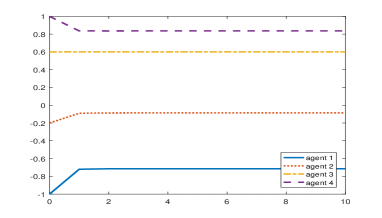
(b) $\Lambda=I-\mathop{\rm diag}\nolimits(W)$

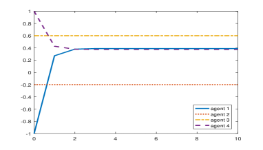
(c) $\Lambda=\mathop{\rm diag}\nolimits(1,0,0,1)$

Figure 6: Opinion dynamics for $W$ from (24) and different $\Lambda$.

6.2 Friedkin’s influence centrality and PageRank

A natural question arises whether the concept of social power, introduced for the French-DeGroot model, can be extended to the model (20). In this subsection, we discuss such an extension, introduced by Friedkin [129, 19] and based on the equality (23). We confine ourselves to the case of asymptotically stable model (20) with the prejudice vector $u=x(0)$, hence $x(\infty)=Vx(0)$, where $V=(I-\Lambda W)^{-1}(I-\Lambda)$.

Recall that the definition of French’s social power assumed that the agents converge to the same consensus opinion $x_{1}(\infty)=\ldots=x_{n}(\infty)$; the social power of agent $i$ is defined as the weight of its initial opinion $x_{i}(0)$ in this final opinion of the group. The Friedkin-Johnsen model provides a generalization of social power of agent $i$ as the mean weight of its initial opinion in determining group members’ final opinions [19]. Mathematically, these mean influence weights are elements of the non-negative vector $c\stackrel{{\scriptstyle\Delta}}{{=}}n^{-1}V^{\top}\mathbbm{1}_{n}$, which satisfies the following equality

$$\bar{x}=\frac{1}{n}\sum_{i=1}^{n}x_{i}(\infty)=\frac{1}{n}\mathbbm{1}_{n}^{\top}Vx(0)=c^{\top}x(0).$$ (25)

Following [129, 19], we call $c_{i}$ the influence centrality of agent $i$. Since $V$ is stochastic, $c^{\top}\mathbbm{1}_{n}=1$. Similar to French’s social power, the influence centrality is generated by an opinion formation mechanism.

Choosing a stochastic matrix $W$, adapted to a given graph $\mathcal{G}$ with $n$ nodes, and some diagonal matrix $\Lambda$, Friedkin’s construction gives a very insightful and broad class of centrality measures. For a fixed $W$, let $\Lambda=\alpha I_{n}$ with $\alpha\in(0,1)$ and consider the corresponding matrix $V_{\alpha}$ and vector $c_{\alpha}$. Obviously, $c_{0}=n^{-1}\mathbbm{1}_{n}$, i.e. the social power is uniformly distributed between all agents. As $\alpha\to 1$, the vector $c_{\alpha}$ converges to French’s social power (when it exists).

Lemma 24

Let $W$ be a fully regular matrix and $p_{\infty}$ stand for the vector of French’s social power, corresponding to the model (2). Then, $p_{\infty}=\lim\limits_{\alpha\to 1-0}c_{\alpha}$.

Indeed, as follows from [63, Eq. (12)] $V_{\alpha}=(1-\alpha)(I-\alpha W)^{-1}\xrightarrow[\alpha\to 1-]{}W^{\infty}$, where $W^{\infty}=\lim\limits_{k\to\infty}W^{k}=\mathbbm{1}_{n}p^{\top}$. Thus $c_{\alpha}=n^{-1}V^{\top}_{\alpha}\mathbbm{1}_{n}\xrightarrow[\alpha\to 1-]{}p_{\infty}$.

The class of Friedkin’s centrality measures $f_{\alpha}$ contains the well-known PageRank [130, 131, 132, 133, 134, 135, 136], proposed originally for ranking webpages in Web search engines and used in scientometrics for journal ranking [133]. The relation between the influence centrality and PageRank, revealed in [137], follows from the construction of PageRank via “random surfing” [131].

Consider a segment of World Wide Web (WWW) with $n$ webpages and a stochastic $n\times n$ hyperlink matrix $W=(w_{ij})$, where $w_{ij}>0$ if and only if a hyperlink leads from the $i$th webpage to the $j$th one. Reaching webpage $i$, the surfer randomly follows one of the hyperlinks on it; the probability to choose the hyperlink leading to webpage $j$ is $w_{ij}$ (the webpage may refer to itself $w_{ii}>0$). Such a process of random surfing is a Markov process; denoting the probability to open webpage $i$ on step $k$ by $p_{i}(k)$, the row vector $p(k)^{\top}=(p_{1}(k),\ldots,p_{n}(k))$ obeys the “dual” French-DeGroot model (7). As discussed in Section 6, if the French social power vector $p_{\infty}$ is well-defined, then the probability distribution $p(k)$ converges to $p_{\infty}$. Since $p_{\infty}^{\top}=p^{\top}W$, the vector $p_{\infty}$ satisfies the natural principle of webpage ranking: a webpage referred by highly ranked webpages should also get a high rank. However, the web graphs are often disconnected, so $W$ may be not fully regular, i.e. the French’s social power may not exist. To avoid this problem, the Markov process of random surfing is modified, allowing the teleportation [131] from each node to a randomly chosen webpage. With probability $m\in(0,1)$, at each step the surfer “gets tired” and opens a random webpage, sampled from the uniform distribution. The Markov chain (7) is replaced by

$$p(k+1)^{\top}=(1-m)p(k)^{\top}W+\frac{m}{n}\mathbbm{1}_{n}^{\top},$$ (26)

which is dual to the Friedkin-Johnsen model (20) with $\Lambda=(1-m)I_{n}$. It can be easily shown that $p(k)^{\top}\to c_{1-m}^{\top}=\frac{m}{n}\mathbbm{1}_{n}^{\top}(1-(1-m)W)^{-1}$. Being a special case of Friedkin’s influence centrality, this limit probability is referred to as PageRank [131, 133] (the Google algorithm [130] used the value $m=0.15$). Another extension of the PageRank centrality, based on the general model (20), has been proposed in [138].

6.3 Alternative interpretations and extensions

Obviously, the French-DeGroot model (2) can be considered as a degenerate case of (20) with $\Lambda=I_{n}$. The French-DeGroot model with stubborn agents, examined in Subsect. 3.6, may be transformed to the more insightful model (20), where $\lambda_{i}=0$ and $u_{i}=x_{i}(0)$ when agent $i$ is stubborn ($w_{ii}=1$) and $\lambda_{i}=1$, $u_{i}=0$ otherwise. Under the assumption of Corollary 14, the system (20) is asymptotically stable and the final opinion vector $x(\infty)=Vu$ is determined by the stubborn agents’ opinions. On the other hand, (20) may be considered as an “augmented” French-DeGroot model with “virtual” $n$ stubborn agents, anchored at $x_{n+i}\equiv u_{i}$ (here $i=1,\ldots,n$).

The model (20) has an elegant game-theoretic interpretation [139, 140]. Suppose that each agent is associated to a cost function $J_{i}(x)=\lambda_{i}\sum_{j=1}^{n}w_{ij}(x_{j}-x_{i})^{2}+(1-\lambda_{i})(x_{i}-u_{i})^{2}$: the first term penalizes the disagreement from the others’ opinions, whereas the other term “anchors” the agent to its prejudice. The update rule (20) implies that each agent $i$ updates its opinion in a way to minimize $J_{i}(x)$, assuming that $x_{j}(k)$, $j\neq k$, are constant. If the system is convergent, the vector $x(\infty)$ stands for the Nash equilibrium [139] in the game, which however does not optimize the overall cost functional $J(x)=\sum_{i}J_{i}(x)$. Some estimates for the ratio $\frac{J(x(\infty))}{\min_{x}J(x)}$ (considered as the “price of anarchy”) are given in [139]. In some special cases the model (20) can also be interpreted in terms of electric circuits [140, 134].

The model (20) with scalar opinions can be extended to $d$-dimensional opinions; similarly to the DeGroot model (4), these opinions can be wrapped into a $n\times d$ matrix $X(k)$, whose $i$th row $x^{i}(k)$ represents the opinion of agent $i$; the multidimensional prejudices are represented by the matrix $U$. The process of opinion formation is thus governed by the model

$$X(k+1)=\Lambda WX(k)+(I-\Lambda)U.$$ (27)

Similar to the multidimensional Taylor model in Subsect. 5.3, the model (27) may be considered as a discrete-time containment control algorithm [141]. An important extension of the model (27), proposed in [63, 142] considers the case where an individual vector-valued opinion represents his/her positions on several interdependent topics (such opinions can stand e.g. for belief systems, obeying some logical constraints [143, 142]). The mutual dependencies between the topics can be described by introducing additional “internal” couplings, described by a stochastic $d\times d$ matrix $C$. The model (27) is replaced by

$$X(k+1)=\Lambda WX(k)C^{\top}+(I-\Lambda)U.$$ (28)

As shown in [63], the stability conditions for (28) remain the same as for the original model (20). In [142] (see also Supplement to this paper) an extension of (28) has been also examined, where agents’ have heterogeneous sets of logical constraints, corresponding to $n$ different coupling matrices $C_{1},\ldots,C_{n}$.

Finally, gossip-based versions of the models (20) and (28) with asynchronous communication have been proposed in [128, 135, 134, 63]; these models will be considered in Part II of this tutorial.

Concluding Remarks and Acknowledgements

In the first part of the tutorial, we have discussed several dynamic models, in continuous and discrete-time, for opinion formation and evolution. A rigorous analysis of the convergence and stability properties of these models is provided, the relations with recent results on multi-agent systems are discussed. Due to the page limit, we do not discuss some important “scalability” issues, regarding the applicability of the models to large-scale social networks. Among such issues are the algorithmic analysis of convergence conditions [144], the models’ convergence rates [145, 146, 140, 147, 148] and experimental validation on big data [149]. An important open problem is to find the relation between the behavior of opinions in the models from Sections 3-6 and the structure of communities or modules in the network’s graph [150].

In the second part of the tutorial, we are going to discuss advanced more advanced models of opinion formation, based on the ideas of bounded confidence [92, 151, 152], antagonistic interactions [153, 154, 155] and asynchronous gossip-based interactions [156, 134]. Future perspectives of systems and control in social and behavioral sciences will also be discussed.

The authors are indebted to Prof. Noah Friedkin, Prof. Francesco Bullo, Dr. Paolo Frasca and the anonymous reviewers for their invaluable comments.

References

- [1] K. Lewin, Frontiers in group dynamics: Concept, method and reality in social science; social equilibria and social change, Human Relations 1 (5) (1947) 5–41.
- [2] J. Moreno, Who Shall Survive? A New Approach to the Problem of Human Interrelations, Nervous and Mental Disease Publishing Co., Washington, D.C., 1934.
- [3] J. Moreno, Sociometry, Experimental Method, and the Science of Society, Beacon House, Ambler, PA, 1951.
- [4] S. Wasserman, K. Faust, Social Network Analysis: Methods and Applications, Cambridge Univ. Press, Cambridge, 1994.
- [5] J. Scott, Social Network Analysis, SAGE Publications, 2000.
- [6] L. Freeman, The Development of Social Network Analysis. A Study in the Sociology of Science, Empirical Press, Vancouver, BC Canada, 2004.
- [7] J. Scott, P. Carrington (Eds.), The SAGE Handbook on Social Network Analysis, SAGE Publications, 2011.
- [8] M. Diani, D. McAdam (Eds.), Social Movements and Networks, Oxford Univ. Press, Oxford, 2003.
- [9] D. Easley, J. Kleinberg, Networks, Crowds and Markets. Reasoning about a Highly Connected World, Cambridge Univ. Press, Cambridge, 2010.
- [10] M. Jackson (Ed.), Social and Economic Networks, Princeton Univ. Press, Princeton and Oxford, 2008.
- [11] D. Knoke, Political Networks. The Structural Perspective, Cambridge Univ. Press, 1993.
- [12] A. O’Malley, P. Marsden, The analysis of social networks, Health Serv. Outcomes Res. Method. 8 (4) (2008) 222–269.
- [13] S. Strogatz, Exploring complex networks, Nature 410 (2001) 268–276.
- [14] M. Newman, The structure and function of complex networks, SIAM Rev. 45 (2) (2003) 167–256.
- [15] M. Newman, A. Barabasi, D. Watts, The Structure and Dynamics of Networks, Princeton Univ. Press, 2006.
- [16] N. Wiener, Cybernetics, or Control and Communications in the Animal and the Machine, Wiley & Sons, New York, 1948.
- [17] N. Wiener, The Human Use of Human Beings: Cybernetics and Society, Houghton Mifflin, New Haven, 1954.
- [18] F. Geyer, The challenge of sociocybernetics, Kybernetes 24 (4) (1995) 6–32.
- [19] N. Friedkin, The problem of social control and coordination of complex systems in sociology: A look at the community cleavage problem, IEEE Control Syst. Mag. 35 (3) (2015) 40–51.
- [20] R. Murray (Ed.), Control in an Information Rich World: Report of the Panel on Future Directions in Control, Dynamics and Systems, SIAM, Philadelphia, PA, 2003.
- [21] T. Samad, A. Annaswamy (Eds.), The Impact of Control Technology. Overview, Success Stories, and Research Challenges, IEEE Control Systems Society, 2011.
- [22] A. Annaswamy, T. Chai, S. Engell, S. Hara, A. Isaksson, P. Khargonekar, F. Lamnabhi-Lagarrigue, R. Murray, H. Nijmeijer, T. Samad, D. Tilbury, P. V. den Hof, Systems & control for the future of humanity. Research agenda: current and future roles, impact and grand challenges, to be published in Annual Reviews in Control.
- [23] S. Strogatz, Sync: The Emerging Science of Spontaneous Order, Hyperion Press, New York, 2003.
- [24] P. Sorokin, Society, Culture, and Personality: Their Structure and Dynamics, a System of General Sociology, Harper & Brothers Publ., New York & London, 1947.
- [25] R. Breiger, K. Carley, P. Pattison (Eds.), Dynamic Social Network Modeling and Analysis: Workshop Summary and Papers, National Acad. Press, Washington, DC, 2003.
- [26] P. Holme, J. Saramäki (Eds.), Temporal Networks, Springer-Verlag, Berlin Heidelberg, 2013.
- [27] C. Aggarwal, K. Subbian, Evolutionary network analysis: A survey, ACM Comput. Surveys 47 (1) (2014) 1–36.
- [28] W. Weidlich, Thirty years of sociodynamics. An integrated strategy of modelling in the social sciences: applications to migration and urban evolution, Chaos, Solitons and Fractals 24 (2005) 45–56.
- [29] C. Castellano, S. Fortunato, V. Loreto, Statistical physics of social dynamics, Rev. Mod. Phys. 81 (2009) 591–646.
- [30] V. Arnaboldi, A. Passarella, M. Conti, R. Dunbar, Online Social Networks. Human Cognitive Constraints in Facebook and Twitter Personal Graphs, Elsevier, New York, NY, 2015.
- [31] W. Mason, F. Conrey, E. Smith, Situating social influence processes: Dynamic, multidirectional flows of influence within social networks, Personal. Soc. Psychol. Rev. 11 (2007) 279–300.
- [32] D. Acemoglu, M. Dahleh, I. Lobel, A. Ozdaglar, Bayesian learning in social networks, Rev. Econom. Studies 78 (4) (2011) 1201–1236.
- [33] H. Xia, H. Wang, Z. Xuan, Opinion dynamics: A multidisciplinary review and perspective on future research, Int. J. Knowledge Systems Sci. 2 (4) (2011) 72–91.
- [34] R. Abelson, Mathematical models of the distribution of attitudes under controversy, in: N. Frederiksen, H. Gulliksen (Eds.), Contributions to Mathematical Psychology, Holt, Rinehart & Winston, Inc, New York, 1964, pp. 142–160.
- [35] J. Hunter, J. Danes, S. Cohen, Mathematical Models of Attitude Change, vol.1, Acad. Press, Inc., 1984.
- [36] S. Kaplowitz, E. Fink, Dynamics of attitude change, in: R. Levine, H. Fitzgerald (Eds.), Analysis of Dynamic Psychological Systems. Vol. 2: Methods and Applications, Plenum Press, New York and London, 1992.
- [37] J. Y. Halpern, The relationship between knowledge, belief, and certainty, Annals of Mathematics and Artificial Intelligence 4 (3) (1991) 301–322.
- [38] M. DeGroot, Reaching a consensus, Journal of the American Statistical Association 69 (1974) 118–121.
- [39] L. Li, A. Scaglione, A. Swami, Q. Zhao, Consensus, polarization and clustering of opinions in social networks, IEEE J. on Selected Areas in Communications 31 (6) (2013) 1072–1083.
- [40] W. Weidlich, The statistical description of polarization phenomena in society, Br. J. Math. Stat. Psychol. 24 (1971) 251–266.
- [41] P. Clifford, A. Sudbury, A model for spatial conflict, Biometrika 60 (3) (1973) 581–588.
- [42] M. Granovetter, Threshold models of collective behavior, Amer. J. Sociology 83 (6) (1978) 1420–1443.
- [43] R. Holley, T. Liggett, Ergodic theorems for weakly interacting infinite systems and the voter model, The Annals of Probability 3 (4) (1975) 643–663.
- [44] K. Sznajd-Weron, J. Sznajd, Opinion evolution in closed community, Int. J. Mod. Phys. C 11 (06) (2000) 1157–1165.
- [45] E. Yildiz, A. Ozdaglar, D. Acemoglu, A. Saberi, A. Scaglione, Binary opinion dynamics with stubborn agents, ACM Transactions on Economics and Computation 1 (4) (2013) article No. 19.
- [46] R. Axelrod, The dissemination of culture: A model with local convergence and global polarization, J. Conflict Resolut. 41 (1997) 203–226.
- [47] C. Canuto, F. Fagnani, P. Tilli, An Eulerian approach to the analysis of Krause’s consensus models, SIAM J. Control Optim. 50 (2012) 243–265.
- [48] A. Mirtabatabaei, P. Jia, F. Bullo, Eulerian opinion dynamics with bounded confidence and exogenous inputs, SIAM J. Appl. Dynam. Syst. 13 (1) (2014) 425–446.
- [49] J. Maynard Smith, Evolution and the Theory of Games, Cambridge Univ. Press, 1982.
- [50] N. Rashevsky, Studies in mathematical theory of human relations, Psychometrika 4 (3) (1939) 221–239.
- [51] N. Rashevsky, Mathematical Theory of Human Relations, Principia Press, Bloomington, 1947.
- [52] R. Abelson, Mathematical models in social psychology, in: L. Berkowitz (Ed.), Advances in Experimental Social Psychology, v. 3, Acad. Press, New York, 1967, pp. 1–49.
- [53] F. Harary, R. Norman, D. Cartwright, Structural Models. An Introduction to the Theory of Directed Graphs, Wiley & Sons, 1965.
- [54] W. T. Tutte, Graph Theory, Addison-Wesley, 1984.
- [55] F. Bullo, Lectures on Network Systems, published online at http://motion.me.ucsb.edu/book-lns, 2016, with contributions by J. Cortes, F. Dorfler, and S. Martinez.
- [56] W. Ren, R. Beard, Distributed Consensus in Multi-Vehicle Cooperative Control: Theory and Applications, Springer-Verlag, London, 2008.
- [57] W. Ren, Y. Cao, Distributed Coordination of Multi-agent Networks, Springer, 2011.
- [58] P. Chebotarev, R. Agaev, Forest matrices around the Laplacian matrix, Linear Algebra Appl. 356 (2002) 253–274.
- [59] A. Berman, R. Plemmons, Nonnegative matrices in the mathematical sciences, Acad. Press, New York, 1979.
- [60] R. Horn, C. Johnson, Matrix Analysis, Cambridge Univ. Press, 1985.
- [61] C. Meyer, Matrix Analysis and Applied Linear Algebra, SIAM, 2000.
- [62] F. Gantmacher, The Theory of Matrices, Vol. 2, AMS Chelsea Publishing, 2000.
- [63] S. Parsegov, A. Proskurnikov, R. Tempo, N. Friedkin, Novel multidimensional models of opinion dynamics in social networks, IEEE Trans. Autom. Control 62 (5) (2017) (published online).
- [64] C. Godsil, G. Royle, Algebraic Graph Theory, Springer-Verlag New York, Inc., 2001.
- [65] R. Agaev, P. Chebotarev, On the spectra of nonsymmetric Laplacian matrices, Linear Algebra Appl. 399 (2005) 157–168.
- [66] W. Ren, R. Beard, Consensus seeking in multiagent systems under dynamically changing interaction topologies, IEEE Trans. Autom. Control 50 (5) (2005) 655–661.
- [67] Z. Lin, B. Francis, M. Maggiore, Necessary and sufficient graphical conditions for formation control of unicycles, IEEE Trans. Autom. Control 50 (1) (2005) 121–127.
- [68] J. French Jr., A formal theory of social power, Physchol. Rev. 63 (1956) 181–194.
- [69] K. Lehrer, When rational disagreement is impossible, Noûs 10 (3) (1976) 327–332.
- [70] C. Wagner, Consensus through respect: A model of rational group decision-making, Philosophical Studies: An International Journal for Philosophy in the Analytic Tradition 34 (4) (1978) 335–349.
- [71] K. Lehrer, C. Wagner, Rational Consensus in Science and Society, D. Reidel Publ., 1981.
- [72] B. Golub, M. O. Jackson, Naive learning in social networks and the wisdom of crowds, American Economic Journal: Microeconomics 2 (1) (2010) 112–149.
- [73] A. Jadbabaie, P. Molavi, A. Sandroni, A. Tahbaz-Salehi, Non-Bayesian social learning, Games and Economic Behavior 76 (2012) 210–225.
- [74] J. French, B. Raven, The bases of social power, in: D. Cartwright (Ed.), Studies in Social Power, Univ. of Michigan Press, Ann Arbor, MI, 1959, pp. 251–260.
- [75] N. Friedkin, A formal theory of social power, J. of Math. Sociology 12 (2) (1986) 103–126.
- [76] F. Harary, A criterion for unanimity in French’s theory of social power, in: D. Cartwright (Ed.), Studies in Social Power, Univ. of Michigan Press, Ann Arbor, MI, 1959, pp. 168–182.
- [77] E. Eisenberg, D. Gale, Consensus of subjective probabilities: the Pari-Mutuel method, The Annals of Math. Stat. 30 (1959) 165–168.
- [78] J. Nash, Non-cooperative games, The Annals of Mathematics 54 (2) (1951) 286–295.
- [79] K. Jain, V. Vazirani, Eisenberg–Gale markets: Algorithms and game-theoretic properties, Games and Economic Behavior 70 (1) (2010) 84–106.
- [80] R. Winkler, The consensus of subjective probability distributions, Management Science 15 (2) (1968) B61–B75.
- [81] M. Stone, The opinion pool, The Annals of Math. Stat. 32 (1961) 1339–1342.
- [82] E. Seneta, Non-Negative Matrices and Markov Chains, 2nd ed., Springer-Verlag, New York, 1981.
- [83] F. Kemeny, J. Snell, Finite Markov Chains, Springer Verlag, New York, Berlin, Heidelberg, Tokyo, 1976.
- [84] J. Wolfowitz, Products of indecomposable, aperiodic, stochastic matrices, Proceedings of Amer. Math. Soc. 15 (1963) 733–737.
- [85] A. Jadbabaie, J. Lin, A. Morse, Coordination of groups of mobile autonomous agents using nearest neighbor rules, IEEE Trans. Autom. Control 48 (6) (2003) 988–1001.
- [86] P. DeMarzo, D. Vayanos, J. Zwiebel, Persuasion bias, social influence, and unidimensional opinions, Quaterly J. Econom. 118 (3) (2003) 909–968.
- [87] J. Tsitsiklis, D. Bertsekas, M. Athans, Distributed asynchronous deterministic and stochastic gradient optimization algorithms, IEEE Trans. Autom. Control 31 (9) (1986) 803–812.
- [88] V. Blondel, J. Hendrickx, A. Olshevsky, J. Tsitsiklis, Convergence in multiagent coordination, consensus, and flocking, in: Proc. IEEE Conf. Decision and Control, 2005, pp. 2996 – 3000.
- [89] M. Cao, A. Morse, B. Anderson, Reaching a consensus in a dynamically changing environment: a graphical approach, SIAM J. Control Optim. 47 (2) (2008) 575–600.
- [90] L. Moreau, Stability of multiagent systems with time-dependent communication links, IEEE Trans. Autom. Control 50 (2) (2005) 169–182.
- [91] D. Angeli, P. Bliman, Stability of leaderless discrete-time multi-agent systems, Math. Control, Signals, Syst. 18 (4) (2006) 293–322.
- [92] R. Hegselmann, U. Krause, Opinion dynamics and bounded confidence models, analysis, and simulation, J. Artifical Societies Social Simul. (JASSS) 5 (3) (2002) 2.
- [93] N. Friedkin, P. Jia, F. Bullo, A theory of the evolution of social power: natural trajectories of interpersonal influence systems along issue sequences, Soc. Science 3 (2016) 444–472.
- [94] J. Seneta, Markov chains, Cambridge Univ. Press, 1998.
- [95] P. Bonacich, P. Lloyd, Eigenvector-like measures of centrality for asymmetric relations, Social Networks 23 (2001) 191–201.
- [96] M. Newman, The structure and function of complex networks, SIAM Rev. 45 (2) (2003) 167–256.
- [97] R. Hegselmann, U. Krause, Opinion dynamics under the influence of radical groups, charismatic leaders and other constant signals: a simple unifying model, Networks and Heterogeneous Media 10 (3) (2015) 477–509.
- [98] N. Masuda, Opinion control in complex networks, New J. Phys. 17 (3) (2015) 033031.
- [99] T. Kurahashi-Nakamura, M. Mäs, J. Lorenz, Robust clustering in generalized bounded confidence models, J. Artificial Societies and Social Simulation 19 (4) (2016) 7.
- [100] R. Olfati-Saber, R. Murray, Consensus problems in networks of agents with switching topology and time-delays, IEEE Trans. Autom. Control 49 (9) (2004) 1520–1533.
- [101] M. Mesbahi, M. Egerstedt, Graph Theoretic Methods in Multiagent Networks, Princeton University Press, Princeton and Oxford, 2010.
- [102] P. Chebotarev, R. Agaev, The forest consensus theorem, IEEE Trans. Autom. Control 59 (9) (2014) 2475–2479.
- [103] L. Moreau, Stability of continuous-time distributed consensus algorithms, in: Proc. IEEE Conf. Decision and Control (CDC 2004), 2004, pp. 3998 – 4003.
- [104] J. Hendrickx, J. Tsitsiklis, Convergence of type-symmetric and cut-balanced consensus seeking systems, IEEE Trans. Autom. Control 58 (1) (2013) 214–218.
- [105] A. Matveev, I. Novinitsyn, A. Proskurnikov, Stability of continuous-time consensus algorithms for switching networks with bidirectional interaction, in: Proc. Europ. Control Conference (ECC), 2013, pp. 1872–1877.
- [106] S. Martin, A. Girard, Continuous-time consensus under persisten connectivity and slow divergence of reciprocal interaction weights, SIAM J. Control. Optim. 51 (3) (2013) 2568–2584.
- [107] S. Martin, J. Hendrickx, Continuous-time consensus under non-instantaneous reciprocity, IEEE Trans. Autom. Control 61 (9) (2016) 2484–2495.
- [108] A. Proskurnikov, A. Matveev, M. Cao, Opinion dynamics in social networks with hostile camps: Consensus vs. polarization, IEEE Trans. Autom. Control 61 (6) (2016) 1524–1536.
- [109] F. Lewis, H. Zhang, K. Hengster-Movris, A. Das, Cooperative Control of Multi-Agent Systems. Optimal and Adaptive Design Approaches, Springer-Verlag, London, 2014.
- [110] A. Proskurnikov, M. Cao, Consensus in multi-agent systems, in: J. Webster (Ed.), Wiley Encyclopedia of Electrical and Electronics Engineering, Wiley & Sons, 2016.
- [111] Z. Li, Z. Duan, G. Chen, L. Huang, Consensus of multiagent systems and synchronization of complex networks: A unified viewpoint, IEEE Trans. on Circuits and Systems - I 57 (1) (2010) 213–224.
- [112] Z. Lin, B. Francis, M. Maggiore, State agreement for continuous-time coupled nonlinear systems, SIAM J. Control Optim. 46 (1) (2007) 288–307.
- [113] U. Münz, A. Papachristodoulou, F. Allgöwer, Consensus in multi-agent systems with coupling delays and switching topology, IEEE Trans. Autom. Control 56 (12) (2011) 2976–2982.
- [114] W. Xia, M. Cao, Clustering in diffusively coupled networks, Automatica 47 (11) (2011) 2395–2405.
- [115] M. Taylor, Towards a mathematical theory of influence and attitude change, Human Relations 21 (2) (1968) 121–139.
- [116] M. Ji, G. Ferrari-Trecate, M. Egerstedt, A. Buffa, Containment control in mobile networks, IEEE Trans. Autom. Control 53 (8) (2008) 1972–1975.
- [117] H. Liu, G. Xie, L. Wang, Necessary and sufficient conditions for containment control of networked multi-agent systems, Automatica 48 (7) (2012) 1415–1422.
- [118] Y. Cao, Consensus of multi-agent systems with state constraints: A unified view of opinion dynamics and containment control, in: Proc. of Amer. Control Conf. (ACC), 2015, pp. 1439–1444.
- [119] Y. Cao, W. Ren, M. Egerstedt, Distributed containment control with multiple stationary or dynamic leaders in fixed and switching directed networks, Automatica 48 (8) (2012) 1586–1597.
- [120] G. Shi, Y. Hong, K. Johansson, Connectivity and set tracking of multi-agent systems guided by multiple moving leaders, IEEE Trans. Autom. Control 57 (2012) 663–676.
- [121] G. Shi, Y. Hong, Global target aggregation and state agreement of nonlinear multi-agent systems with switching topologies, Automatica 45 (5) (2009) 1165–1175.
- [122] G. Shi, K. Johansson, Y. Hong, Reaching an optimal consensus: Dynamical systems that compute intersections of convex sets, IEEE Trans. on Autom. Control 58 (3) (2013) 610–622.
- [123] N. Friedkin, E. Johnsen, Social influence and opinions, J. Math. Sociol. 15 (3-4) (1990) 193–205.
- [124] N. Friedkin, A Structural Theory of Social Influence, Cambridge Univ. Press, New York, 1998.
- [125] N. Friedkin, E. Johnsen, Social influence networks and opinion change, in: S. Thye, E. Lawler, M. Macy, H. Walker (Eds.), Advances in Group Processes, Vol. 16, 1999, pp. 1–29.
- [126] C. Childress, N. Friedkin, Cultural reception and production, Amer. Soc. Rev. 77 (2012) 45–68.
- [127] N. Friedkin, E. Johnsen, Social Influence Network Theory, Cambridge Univ. Press, New York, 2011.
- [128] P. Frasca, C. Ravazzi, R. Tempo, H. Ishii, Gossips and prejudices: Ergodic randomized dynamics in social networks, in: Proc. of IFAC NecSys 2013 Workshop, Koblenz, Germany, 2013, pp. 212–219.
- [129] N. Friedkin, Theoretical foundations for centrality measures, Amer. J. Sociology 96 (6) (1991) 1478–1504.
- [130] S. Brin, L. Page, The anatomy of a large-scale hypertextual Web search engine, Computer Networks and ISDN Systems archive 30 (1998) 107–117.
- [131] P. Boldi, M. Santini, S. Vigna, PageRank: Functional dependencies, ACM Trans. Inform. Syst. 27 (4) (2009) 1–23.
- [132] H. Ishii, R. Tempo, Distributed randomized algorithms for the PageRank computation, IEEE Trans. Autom. Control 55 (9) (2010) 1987–2002.
- [133] H. Ishii, R. Tempo, The PageRank problem, multi-agent consensus and Web aggregation: A systems and control viewpoint, IEEE Control Syst. Mag. 34 (3) (2014) 34–53.
- [134] P. Frasca, H. Ishii, C. Ravazzi, R. Tempo, Distributed randomized algorithms for opinion formation, centrality computation and power systems estimation: A tutorial overview, Europ. J. Control 24 (7) (2015) 2–13.
- [135] C. Ravazzi, P. Frasca, R. Tempo, H. Ishii, Ergodic randomized algorithms and dynamics over networks, IEEE Trans. Control of Network Syst. 2 (1) (2015) 78–87.
- [136] K. You, R. Tempo, L. Qiu, Distributed algorithms for computation of centrality measures in complex networks, IEEE Trans. Autom. Control (published online).
- [137] N. Friedkin, E. Johnsen, Two steps to obfuscation, Social Networks 39 (2014) 12–13.
- [138] A. Proskurnikov, R. Tempo, M. Cao, PageRank and opinion dynamics: Missing links and extensions, in: Proc. of IEEE Conf. Norbert Wiener in the 21st Century, Melbourne, 2016, pp. 12–17.
- [139] D. Bindel, J. Kleinberg, S. Oren, How bad is forming your own opinion?, in: Proc. of IEEE Symp. on Foundations of Computer Science, 2011, pp. 57–66.
- [140] J. Ghaderi, R. Srikant, Opinion dynamics in social networks with stubborn agents: Equilibrium and convergence rate, Automatica 50 (12) (2014) 3209–3215.
- [141] X. Mu, Z. Yang, Containment control of discrete-time general linear multi-agent systems under dynamic digraph based on trajectory analysis, Neurocomputing 171 (2016) 1655–1660.
- [142] N. Friedkin, A. Proskurnikov, R. Tempo, S. Parsegov, Network science on belief system dynamics under logic constraints, Science 354 (6310) (2016) 321–326.
- [143] P. Converse, The nature of belief systems in mass publics, in: D. Apter (Ed.), Ideology and Discontent, Free Press, New York, 1964, pp. 206–261.
- [144] J. Jarvis, D. Shier, Graph-theoretic analysis of finite Markov chains, in: D. Shier, K. Wallenius (Eds.), Applied Mathematical Modeling: A Multidisciplinary Approach, Chapman & Hall/CRC, 2000.
- [145] M. Cao, A. Morse, B. Anderson, Reaching a consensus in a dynamically changing environment: convergence rates, measurement delays, and asynchronous events, SIAM J. Control Optim. 47 (2) (2008) 601–623.
- [146] A. Olshevsky, J. Tsitsiklis, Convergence speed in distributed consensus and averaging, SIAM Rev. 53 (4) (2011) 747–772.
- [147] M. Pirani, S. Sundaram, On the smallest eigenvalue of grounded Laplacian matrices, IEEE Trans. Autom. Control 61 (2) (2016) 509–514.
- [148] A. Proskurnikov, R. Tempo, M. Cao, N. Friedkin, Opinion evolution under time-varying social influence with individual prejudices: from consensus to disagreement, in: Proc. of IFAC World Congress, Toulouse, France, 2017.
- [149] C. Vande Kerckhove, S. Martin, P. Gend, P. Rentfrow, J. Hendrickx, V. Blondel, Modelling influence and opinion evolution in online collective behaviour, PLoS One 11 (6) (2016) e0157685.
- [150] S. Fortunato, Community detection in graphs, Physics Reports 486 (3–5) (2010) 75–174.
- [151] V. Blondel, J. Hendrickx, J. Tsitsiklis, Continuous-time average-preserving opinion dynamics with opinion-dependent communications, SIAM J. Control Optim. 48 (2010) 5214–5240.
- [152] I. C. Morarescu, A. Girard, Opinion dynamics with decaying confidence: Application to community detection in graphs, IEEE Transactions on Automatic Control 56 (8) (2011) 1862–1873.
- [153] C. Altafini, Dynamics of opinion forming in structurally balanced social networks, PLoS ONE 7 (6) (2012) e38135.
- [154] C. Altafini, Consensus problems on networks with antagonistic interactions, IEEE Trans. Autom. Control 58 (4) (2013) 935–946.
- [155] G. Shi, A. Proutiere, M. Johansson, J. Baras, K. Johansson, The evolution of beliefs over signed social networks, Oper. Res. 64 (3) (2016) 585–604.
- [156] G. Deffuant, D. Neau, F. Amblard, G. Weisbuch, Mixing beliefs among interacting agents, Advances in Complex Systems 3 (2000) 87–98.