West University of Timişoara
Department of Physics

MASTER THESIS

SUPERVISOR,
Lect.dr. NICOLAEVICI NISTOR

AUTHOR,
AMBRUŞ VICTOR EUGEN

Timişoara
2010

West University of Timişoara
Department of Physics

PARTICLE PRODUCTION IN
A ROBERTSON-WALKER SPACE
WITH A DE SITTER PHASE
OF FINITE EXTENSION

SUPERVISOR,
Lect.dr. NICOLAEVICI NISTOR

AUTHOR,
AMBRUŞ VICTOR EUGEN

Timişoara
2010

Abstract

We investigate the phenomenon of particle production in a Friedmann-Robertson-Walker universe which contains a phase of de Sitter expansion for a finite interval, outside which it reduces to the flat Minkowski spacetime. We compute the particle number density for a massive scalar and a spinorial field and point out differences between the two cases. We find that the resulting particle density approaches a constant value at the scale of the Hubble time and that for a certain choice of the parameters the spectrum is precisely thermal for the spinorial field, and almost thermal for the scalar field.

Contents

1. 1 Introduction
2. 2 Quantum fields on curved spaces
   1. 2.1 Friedmann-Robertson-Walker spaces
   2. 2.2 Quantization procedure
      1. 2.2.1 The Klein-Gordon field
      2. 2.2.2 The Dirac field
   3. 2.3 Particle production
      1. 2.3.1 The Klein-Gordon field
      2. 2.3.2 The Dirac field
3. 3 The free field equation on de Sitter space-time
   1. 3.1 The Klein-Gordon field
   2. 3.2 The Dirac field
   3. 3.3 The Minkowski solutions
4. 4 Creation of massive scalar particles
   1. 4.1 Bogoliubov coefficients
      1. 4.1.1 de Sitter in and out modes
      2. 4.1.2 Mode mixing and density of created particles
      3. 4.1.3 Particle production of conformal massless scalar particles
      4. 4.1.4 Graphical analysis
   2. 4.2 Asymptotic analysis
      1. 4.2.1 Large momentum $p\gg\omega$
      2. 4.2.2 Low momentum $q\ll\omega$
      3. 4.2.3 Middle region $p\ll\omega\ll q$
      4. 4.2.4 The number of created particles
      5. 4.2.5 Graphical comparison to the exact solution
5. 5 Creation of spinorial particles
   1. 5.1 Bogoliubov coefficients
      1. 5.1.1 de Sitter in and out modes
      2. 5.1.2 Mode mixing and density of created particles
      3. 5.1.3 Production of massless Dirac particles
      4. 5.1.4 Graphical analysis
   2. 5.2 Asymptotic analysis
      1. 5.2.1 Large momentum $p\gg\omega$
      2. 5.2.2 Low momentum $q\ll\omega$
      3. 5.2.3 Middle region $p\ll\omega\ll q$
      4. 5.2.4 Resonances
      5. 5.2.5 The number of created particles
      6. 5.2.6 Graphical comparison to the exact solution
6. 6 Conclusion
7. A Properties of Hankel functions
   1. A.1 Differential equation
   2. A.2 Asymptotic forms
   3. A.3 Hankel functions for the de Sitter scalar field
   4. A.4 Hankel functions for the de Sitter spinorial field
8. B Pauli spinors
   1. B.1 Spinor construction
   2. B.2 Behaviour under parity transformations
   3. B.3 Relation between $\xi$ and $\eta$

Chapter 1 Introduction

The keywords describing this thesis are: quantum fields on curved spaces, de Sitter solutions, Bogoliubov transformation, particle production by the coupling with the gravitational field.

Quantum fields on curved spaces are the generalization of the Minkowski quantum theory of fields. The general approach is to consider the space curvature as a background field, described by the metric tensor, which obeys the classical (i.e. not quantum) Einstein field equations. This approach suffers from a number of drawbacks, but it is nevertheless a bold step forward towards the grand unification of all known interactions and the quantization of the gravitational field. History tells us that a new theory is validated against results which are considered as classical. This pseudo-quantum treatment of quantum fields on a curved background provide a good way to produce some classical results.

Working in a background gravitational field is all but easy. With very few exceptions, there are no known analytical solutions to the resulting field equations. One of these exceptions is the de Sitter spacetime, which describes a Friedmann-Robertson-Walker Universe undergoing an exponential expansion [book:MTW, book:birrell_davies].

Even though solutions to field equations might be derived in an external gravitational field, the quantum theory built on them is not as natural and intuitive as it is on Minkowski. For example, the Poincaré invariance of the Minkowski space and of the field equations automatically ensures the existence of “positive” and “negative” frequency states. However, a different choice of coordinate system (e.g. the spherical one), or the coordinates of a non-inertial observer (e.g. the Rindler coordinates) can also be used to define particle states, which might not have the same physical meaning as the former. The accelerated observer detects particles as if he would have been submerged in a thermal bath of temperature related to his own acceleration [book:birrell_davies].

We shall circumvent the more philosophical issues regarding particle states definition and interpretation, and instead consider the space to have only a finite region of a de Sitter expansion phase, outside which the space is flat (see Figure 1.1).

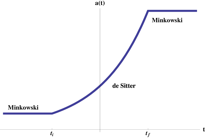
Figure 1.1: The scale factor for the FRW space under consideration

Particle states are only defined on the flat regions of space. The method we employ is to let the in vacuum state evolve through the de Sitter phase, and compute the expectation value of the particle number or the energy density operator in the out region. Poincaré invariance guarantees there is no particle production on the Minkowski regions. This phenomenon takes place only on the de Sitter phase. The particle and anti-particle modes used to construct the solution on de Sitter space are used merely as mathematical tools that allow us to propagate the in modes, and do not receive any physical interpretation as to their particle content. These key ingredients are summarized in Table 2.1.

The purpose of this thesis is to evaluate the density of created particles with given momentum in a unit volume of the out space for a massive scalar and a spinorial field. We find that there is a cutoff for particles with momentum higher than the expansion factor. Using the spectral density we also evaluate the particle number density (per unit volume), and the energy density. We show that the particle number density approaches a constant value as the expansion time approaches the Hubble time, and it increases with the expansion factor and with the mass of the created particles. The energy density is finite only for the case of a conformally coupled massive scalar field, in all other cases (including the spinorial field), it has a logarithmic divergence. It also increases with the expansion factor, and exhibits a higher order increase with respect to the particle mass.

The thesis is structured as follows: chapter 2 presents the spacetime under investigation, after which we recall the basics of the quantization procedure on curved background and the formalism for the description of the particle production phenomenon. A key ingredient in the calculation are the free field equation solutions (the quantum modes), which we present in chapter 3.

Our main result is contained in chapter 4 and chapter 5, where we explicitly obtain the expression for the number density of the created particles. These chapters follow a common pattern for the investigation of scalar and spinorial particle production respectively. Each consists of two sections, the first gives the analytical solution in terms of Hankel functions while the second applies approximation formulas to extract information on the particle production phenomenon. The results obtained are accompanied by a set of figures.

We summarize our results and present our conclusions in chapter 6, where we also point out possibilities for further development.

We have provided Appendix A as a small reference regarding Hankel functions. Appendix B gives insight on the underworks of the Pauli spinors which occur in the polarized solutions of the Dirac equation.

Chapter 2 Quantum fields on curved spaces

This section summarizes the framework and main results needed for the development of the thesis. We assume the reader to be familiar with the quantum theory of free fields and general relativity (good books include [book:itzykson_zuber, book:bjorken_drell, book:MTW, book:wald]). In section 2.1 we present the space-time under consideration and list the results from general relativity which we shall use in subsequent chapters. In section 2.2 we introduce the general formalism for the construction of a quantum field theory on an arbitrary space-time, following the method of [book:birrell_davies]. Other introductory texts include [ebook:ford, ebook:jacobson]. For an introduction to the vierbein formalism, used for the generalization of the Dirac field to curved spaces, the reader can consult [art:cota_external_symm, art:cota_polarized_fermions]. For a modern analysis on the construction of a meaningful symmetric divergenceless stress-energy tensor, we refer to [art:forger_romer].

2.1 Friedmann-Robertson-Walker spaces

The Friedmann-Robertson-Walker space is a spatially isotropic and homogeneous spacetime described by the metric

$$ds^{2}=dt^{2}-a^{2}(t)\boldsymbol{dx}^{2},$$ (2.1.1)

where $a(t)$ is known as the scale factor. Such a space undergous a dilation (or contraction) of distances by the factor $a(t)$. Two special cases of the FRW space are the Minkowski space, which corresponds to

$$a(t)=\text{const},$$ (2.1.2)

and the de Sitter space, which corresponds to

$$a(t)=e^{\omega t}.$$ (2.1.3)

The expansion parameter $\omega$ is also known as the Hubble expansion rate $H$, and the hubble time is defined as $1/H$.

The space we will work with is a FRW space consisting of three regions, as illustrated in Figure 1.1. The continuity of the metric tensor requests $a(t)$ to be a continuous function of $t$, which leads to a line element of the following form:

1. Minkowski in region, $t<t_{i}$:

   $$ds^{2}=dt^{2}-\boldsymbol{dx}_{i}\quad,\quad\boldsymbol{x}_{i}=e^{\omega t_{i}}\boldsymbol{x}$$ (2.1.4a)

2. de Sitter expansion phase, $t_{i}<t<t_{f}$:

   $$ds^{2}=dt^{2}-\boldsymbol{dx}^{2}$$ (2.1.4b)

3. Minkowski in region, $t>t_{f}$:

   $$ds^{2}=dt^{2}-\boldsymbol{dx}_{f}\quad,\quad\boldsymbol{x}_{f}=e^{\omega t_{f}}\boldsymbol{x}$$ (2.1.4c)

We shall refer to $t_{i}$ as the “initial time”, to $t_{f}$ as the “final time” and to $\Delta t=t_{f}-t_{i}$ as the “expansion time”. Note that the effect of the expansion of space is to increase the physical distances, which in turn produces a redshift in particle wavelengths. We shall use “physical quantities” (e.g. physical length, physical momentum) to refer to the results of measurements performed by an observer in a Minkowski region. For example, the momentum operator for the out region is

$$\boldsymbol{P}^{\text{out}}=-i\nabla_{f}=-ie^{-\omega t_{f}}\nabla.$$ (2.1.5)

This is the natural definition of the momentum operator associated with the Killing vector of unit length which generates space translations. The length of the Killing vector is evaluated using the Minkowski metric

$$\eta_{\mu\nu}=\text{diag}(1,-1,-1,-1),$$ (2.1.6)

used for the construction of the line element (2.1.4c). Similarly, the momentum operator for the in region is naturally defined as

$$\boldsymbol{P}^{\text{in}}=-ie^{-\omega t_{i}}\nabla.$$

This establishes the relation between the momentum operators measuring physical momenta in the in and out regions:

$$\boldsymbol{P}^{\text{out}}=e^{-\omega(t_{f}-t_{i})}\boldsymbol{P}^{\text{in}}.$$ (2.1.7)

Particles which have a measured momentum of $p$ in the out region had a measured momentum of

$$\boldsymbol{q}={\boldsymbol{p}}e^{\omega\Delta t}$$ (2.1.8)

in the in region. In terms of the de Sitter momentum ${\boldsymbol{p}}_{\text{dS}}$, given by the Killing vector $-i\partial_{i}$, we have

$$\boldsymbol{q}={\boldsymbol{p}}_{\text{dS}}e^{-\omega t_{i}},\qquad{\boldsymbol{p}}={\boldsymbol{p}}_{\text{dS}}e^{-\omega t_{f}}.$$ (2.1.9)

	in	de Sitter phase	out
time span	$t<t_{i}$	$t_{i}<t<t_{f}$	$t_{f}<t$
$ds^{2}$	$dt^{2}-e^{2\omega t_{i}}\boldsymbol{dx}^{2}$	$dt^{2}-e^{2\omega t}\boldsymbol{dx}^{2}$	$dt^{2}-e^{2\omega t_{f}}\boldsymbol{dx}^{2}$
physical coordinates	$\boldsymbol{x}_{i}=\boldsymbol{x}e^{\omega t_{i}}$	$\boldsymbol{x}e^{\omega t}$	$\boldsymbol{x}_{f}=\boldsymbol{x}e^{\omega t_{f}}$
physical momenta	$q=p_{\text{dS}}e^{-\omega t_{i}}$	$p_{\text{dS}}e^{-\omega t}$	$p=p_{\text{dS}}e^{-\omega t_{f}}$

Table 2.1: summary of the studied space-time

An important feature of FRW spaces is that the metric is conformal with the Minkowski metric, allowing to be cast in the form

$$ds^{2}=a^{2}(\eta)(d\eta^{2}-\boldsymbol{dx}^{2}),\qquad\eta=\int\frac{dt}{a(t)},$$ (2.1.10)

where $\eta$ is called the conformal time. We recall that a conformal transformation may be described by

$$g_{\mu\nu}\mapsto\overline{g}_{\mu\nu}=\Omega^{2}(x)g_{\mu\nu}.$$ (2.1.11)

As the metric undergoes this transformation, all metric-dependent quantities (the connection coefficients, Riemann tensor, curvature) transform in a non-trivial way. In particular, the transformation law for the four-dimensional d’Alembert operator is:

$$\left(\Box+\frac{1}{6}R\right)\phi\mapsto\left(\overline{\Box}+\frac{1}{6}\overline{R}\right)\overline{\phi}\quad,\quad\overline{\phi}(x)=\frac{1}{\Omega}\phi(x).$$ (2.1.12)

All barred quantities are evaluated using the conformally transformed metric (2.1.11). The generally covariant d’Alembert operator on a curved space is

$$\Box\phi=g^{\mu\nu}\nabla_{\mu}\nabla_{\nu}\phi=\frac{1}{\sqrt{-g}}\partial_{\mu}\left(\sqrt{-g}g^{\mu\nu}\partial_{\nu}\phi\right),\qquad g=\det(g_{\mu\nu}).$$ (2.1.13)

This result is of special interest for the theory of scalar fields on curved spaces, described by the lagrangian (2.2.8). If the coupling parameter is set to $\xi=1/6$ (conformal coupling), the massless scalar field obeys a conformal field equation, and thus the solutions are proportional to the Minkowski ones.

The connection coefficients in a coordinate basis $\partial_{\mu}$, also known as Christofell symbols, are defined as

$$\Gamma\indices{{}^{\lambda}_{\mu}{}_{\nu}}=\frac{1}{2}g^{\lambda\kappa}\left(g_{\kappa\mu,\nu}+g_{\kappa\nu,\mu}-g_{\mu\nu,\kappa}\right).$$ (2.1.14)

We shall use these in the construction of the covariant derivative appearing in the d’Alembert operator (2.1.13). In a FRW space of line element (2.1.1) the Christofell symbols are

$$\Gamma\indices{{}^{t}_{i}{}_{j}}=a(t)a^{\prime}(t)\delta_{ij},\qquad\Gamma\indices{{}^{i}_{t}{}_{j}}=\frac{a^{\prime}(t)}{a(t)}\delta\indices{{}^{i}_{j}}.$$ (2.1.15)

The prime denotes differentiation with respect to the argument. In the conformal chart $(\eta,\boldsymbol{x})$, which we shall use in chapter 3, these coefficients read

$$\Gamma\indices{{}^{\eta}_{\eta}{}_{\eta}}=\frac{a^{\prime}(\eta)}{a(\eta)},\qquad\Gamma\indices{{}^{\eta}_{i}{}_{j}}=\frac{a^{\prime}(\eta)}{a(\eta)}\delta_{ij},\qquad\Gamma\indices{{}^{i}_{\eta}{}_{j}}=\frac{a^{\prime}(\eta)}{a(\eta)}\delta\indices{{}^{i}_{j}}.$$ (2.1.16)

The Ricci scalar (the curvature) is given by

$$R=R\indices{{}^{\nu}_{\nu}}=R\indices{{}^{\mu}{}^{\nu}_{\mu}{}_{\nu}}=-6\frac{a^{\prime\prime}}{a}-6\left(\frac{a^{\prime}}{a}\right)^{2}.$$ (2.1.17)

The Minkowski metric $\eta_{\mu\nu}$ (2.1.6) is point-independent ($a(t)=\text{const}$), thus the Christofell symbols (2.1.15) and the Ricci curvature (2.1.17) vanish. In particular, the d’Alembert operator (2.1.13) is the wave operator

$$\Box=\partial_{t}^{2}-\Delta,\qquad\Delta=\sum_{i=1}^{3}\partial^{2}_{i},$$ (2.1.18)

with $\Delta$ being the Laplace operator, acting on all space components. Care must be taken when reading the space coordinates of the Minkowski in and out regions, among which we shall distinguish by appending a subscript _i or _f.

Let us now focus on our case of interest, i.e. that of the de Sitter space (2.1.4b) with the scale factor $a(t)=e^{\omega t}$. The conformal time (2.1.10) is easily integrated to yield

$$\eta=-\frac{1}{\omega}e^{-\omega t},$$ (2.1.19a)

therefore $$a(\eta)=-1/\omega\eta$$. Substituting in (2.1.10), the conformal line element reads

$$ds^{2}=\frac{1}{\omega^{2}\eta^{2}}(d\eta^{2}-\boldsymbol{dx}^{2}).$$ (2.1.19b)

The connection coefficients in this chart are

$$\Gamma\indices{{}^{\eta}_{\eta}{}_{\eta}}=-\frac{1}{\eta},\qquad\Gamma\indices{{}^{\eta}_{i}{}_{j}}=-\frac{1}{\eta}\delta_{ij},\qquad\Gamma\indices{{}^{i}_{\eta}{}_{j}}=-\frac{1}{\eta}\delta\indices{{}^{i}_{j}},$$ (2.1.20)

and the d’Alembert operator is

$$\Box\phi=(\omega^{2}\eta^{2})\left(\partial_{\eta}^{2}-2/\eta\partial_{\eta}-\Delta\right)\phi.$$ (2.1.21)

The Ricci scalar reads

$$R=12\omega^{2}.$$ (2.1.22)

2.2 Quantization procedure

One of the main ingredients in the construction of the quantum field theory in Minkowski spoace is the requirement of Poincaré invariance. In particular, the invariance to time translations allow for the construction of positive and negative frequency modes, which naturally define particle and anti-particle states. This invariance is not guaranteed in general relativity, where the choice of particle states is echivocal. Poincaré inertial observers all agree on the definitions of particles. On the other hand, only a special class of freely falling observers will register the same particle content in a given quantum states.

Following the development in [book:birrell_davies], we shall restrict ourselves to $C^{\infty}$ 4-dimensional, globally hyperbolic, pseudo-Riemannian manifolds. The differentiability conditions ensure the existence of differential equations and the global hyperbolicity ensures the existence of Cauchy hypersurfaces.

The formalism of quantum field theory is generalized to curved spacetime in a straightforward way, but the physical interpretation is not. Except for some cases such as static spacetimes, the physical interpretation of particle states is ambiguous.

In this section we shall outline the general framework of a quantum theory of fields in a background gravitational field, and apply it to general FRW spaces, discussed in section 2.1.

2.2.1 The Klein-Gordon field

The generally covariant action for a charged scalar field is

$$\mathcal{S}[\phi]=\int d^{4}x\sqrt{-g}\left\{g^{\mu\nu}\nabla_{\mu}\phi^{\dagger}(x)\nabla_{\nu}\phi(x)-(m^{2}+\xi R(x))\phi^{\dagger}(x)\phi(x)\right\},$$ (2.2.1a)

and the corresponding field equation is

$$(\Box+m^{2}+\xi R(x))\phi(x)=0\quad,\quad\Box\phi(x)=g^{\mu\nu}\nabla_{\mu}\nabla_{\nu}\phi(x)$$ (2.2.1b)

The most frequently considered values for the coupling parameter are $\xi=0$ (minimal coupling) and $\xi=\nicefrac{{1}}{{6}}$ (conformal coupling). Although the natural coupling to the gravitational field is the minimal one, we shall keep $\xi$ arbitrary when developing the theory. As we shall see, the conformal coupling will emerge as a case of special interest, not only because for this choice the particle production ceasses when the scalar field is massless (see subsection 4.1.3), but also because the energy density of the created particles is at a minimum (see, for example, subsection 4.2.1).

The $\mathcal{U}(1)$ invariance of the action assures the conserved current density

$$\mathfrak{j}^{\mu}=i\sqrt{-g}\,g^{\mu\nu}(\phi^{\dagger}(x)\overleftrightarrow{\partial_{\nu}}\phi(x))\quad,\quad\partial_{\mu}\mathfrak{j}^{\mu}=0,$$ (2.2.2)

and the corresponding current vector

$$j^{\mu}=ig^{\mu\nu}(\phi^{\dagger}(x)\overleftrightarrow{\partial_{\nu}}\phi(x))\quad,\quad\nabla_{\mu}j^{\mu}=0,$$ (2.2.3)

where the bilateral derivative is

$$f\overleftrightarrow{\partial_{\mu}}g=f\partial_{\mu}g-g\partial_{\mu}f.$$ (2.2.4)

The conserved charge follows from (2.2.2)

$$Q=\int j^{\mu}d\Sigma_{\mu},$$ (2.2.5)

where the integral extends over a Cauchy surface. The result is independent of the choice of surface. If we pick $x^{0}$ to be the temporal coordinate, the integral (2.2.5) reads

$$Q=i\int d^{3}x\sqrt{-g}\,g^{\mu 0}(\phi^{\dagger}(x)\overleftrightarrow{\partial_{\mu}}\phi(x)),\qquad\partial_{0}Q=0.$$ (2.2.6)

This suggests to introduce the scalar product

$$\mathinner{\langle{f_{1}},{f_{2}}\rangle}=i\int d^{3}x\sqrt{-g}g^{\mu 0}(f_{1}^{\dagger}(x)\overleftrightarrow{\partial_{\mu}}f_{2}(x)),\qquad\partial_{0}\mathinner{\langle{f_{1}},{f_{2}}\rangle}=0,$$ (2.2.7)

which can be easily shown to be independent of time if and only if $f_{1}(x),f_{2}(x)$ are solutions to the Klein-Gordon equation [ebook:ford]. In the discussion above we referred to a charged scalar field only for establishing the form of the scalar product (2.2.7). In our investigation we shall restrict to the case of an uncharged field (the difference is unessential) for which the Lagrangian density reads

$$\mathcal{L}(\phi,\partial_{\mu}\phi)=\sqrt{-g}\left\{g^{\mu\nu}\frac{1}{2}\nabla_{\mu}\phi(x)\nabla_{\nu}\phi(x)-\frac{1}{2}(m^{2}+\xi R(x))\phi^{2}(x)\right\}.$$ (2.2.8)

The resulting field equation is identical to (2.2.1b), for which the same scalar product (2.2.7) can be introduced.

The conjugate momentum is defined as the derivative of the Lagrangian density (2.2.8) with respect to the time derivative of the field

$$\pi(x)=\frac{\partial\mathcal{L}}{\partial\partial_{0}\phi(x)}=\sqrt{-g}g^{\mu 0}\nabla_{\mu}\phi(x).$$ (2.2.9)

The quantization of the field is achieved by imposing the canonical commutation rules:

$$\mathinner{\left[{\phi(t,\boldsymbol{x})},{\phi(t,\boldsymbol{x}^{\prime})}\right]}=\mathinner{\left[{\pi(t,\boldsymbol{x})},{\pi(t,\boldsymbol{x}^{\prime})}\right]}=0$$ (2.2.10a)

$$\mathinner{\left[{\phi(t,\boldsymbol{x})},{\pi(t,\boldsymbol{x}^{\prime})}\right]}=i\delta^{3}(\boldsymbol{x}-\boldsymbol{x}^{\prime})$$ (2.2.10b)

The field equation is linear, and therefore admits a complete set of solutions, with respect to which the field $\phi(x)$ can be expanded:

$$\phi(x)=\sum_{i}\left(a_{i}f_{i}(x)+a_{i}^{\dagger}f^{*}_{i}(x)\right)$$ (2.2.11)

Since we have a well defined scalar product, we require these modes to satisfy the orthonormalization condition

$$\mathinner{\langle{f_{i}},{f_{j}}\rangle}=\delta_{ij},\qquad\mathinner{\langle{f_{i}},{f_{j}^{*}}\rangle}=0,\qquad\mathinner{\langle{f_{i}^{*}},{f_{j}^{*}}\rangle}=-\delta_{ij}.$$ (2.2.12)

Using the canonical commutation rules (2.2.10) and the completeness relation

$$i\sum_{i}\sqrt{-g}g^{\mu 0}\left(f_{i}^{*}(t,\boldsymbol{x}^{\prime})\partial_{\mu}f_{i}(t,\boldsymbol{x})-f_{i}(x)\partial_{\mu}f^{*}_{i}(t,\boldsymbol{x}^{\prime})\right)=\delta^{3}(\boldsymbol{x}-\boldsymbol{x}^{\prime})$$ (2.2.13)

we arrive at

$$\mathinner{\left[{a^{\phantom{\dagger}}_{i}},{a^{\phantom{\dagger}}_{j}}\right]}=0,\qquad\mathinner{\left[{a^{\dagger}_{i}},{a^{\dagger}_{j}}\right]}=0,\qquad\mathinner{\left[{a_{i}},{a^{\dagger}_{j}}\right]}=\delta_{ij}.$$ (2.2.14)

These operators can be obtained by taking the scalar product between the corresponding mode and the field operator

$$a_{i}=\mathinner{\langle{f_{i}},{\phi}\rangle},\qquad a^{\dagger}_{j}=-\mathinner{\langle{f_{j}^{*}},{\phi}\rangle}.$$ (2.2.15)

The Fock space can be constructed by defining a vacuum (or no-particle) state such that

$$a_{i}\ket{0}=0,\qquad\braket{0}{0}=1.$$ (2.2.16)

With respect to this state, we call $a_{i}$ annihilation operators and $a^{\dagger}_{j}$ creation operators. The former operators annihilate quanta in mode $f_{i}$, while the latter creates quanta in mode $f_{j}$. From the vacuum state, succesive application of the creation operators $a^{\dagger}_{j}$ generates the particle states. The operator that counts the number of particles in a given state is the particle number operator given by

$$N_{i}=a^{\dagger}_{i}a_{i}.$$ (2.2.17)

Finally, the symmetric, divergence-less stress-energy tensor is obtained with the general prescription

$$T_{\mu\nu}=\frac{2}{\sqrt{-g}}\frac{\delta\mathcal{L}}{\delta g^{\mu\nu}}.$$ (2.2.18)

The Lagrangian density (2.2.8) depends on the metric through $\sqrt{-g}$ and through the derivative term. The variation of the latter with respect to the metric is $\sim\nabla_{\mu}\phi\nabla_{\nu}\phi$, while the former’s variation is given by

$$\frac{\delta\sqrt{-g}}{\delta g^{\mu\nu}}=-g_{\mu\nu}\frac{\sqrt{-g}}{2},$$ (2.2.19)

and thus we arrive at

$$T_{\mu\nu}=\nabla_{\mu}\phi\nabla_{\nu}\phi-g_{\mu\nu}\frac{\mathcal{L}}{\sqrt{-g}},$$ (2.2.20)

$$\frac{\mathcal{L}}{\sqrt{-g}}=\frac{1}{2}\left(g^{\mu\nu}\nabla_{\mu}\phi(x)\nabla_{\nu}\phi(x)-(m^{2}+\xi R(x))\phi^{2}(x)\right).$$

There is a problem with this tensor: the energy density of the vacuum state is infinite. However, we are only interested in energy differences, therefore we shall substract the vacuum expectation value and define the new tensor as the normally ordered (Wick ordered) stress-energy tensor:

$$:T_{\mu\nu}:=T_{\mu\nu}-\braket{0}{T_{\mu\nu}}{0}.$$ (2.2.21)

In terms of creation and annihilation operators we have

$$:T_{\mu\nu}:=\sum_{i,j}\left\{a_{i}a_{j}(\partial_{\mu}f_{i}\partial_{\nu}f_{j}-g_{\mu\nu}\mathcal{L}(f_{i},f_{j}))+a^{\dagger}_{i}a^{\dagger}_{j}(\partial_{\mu}f^{*}_{i}\partial_{\nu}f^{*}_{j}-g_{\mu\nu}\mathcal{L}(f^{*}_{i},f^{*}_{j}))\right.\\ \left.+a^{\dagger}_{j}a_{i}(\partial_{\mu}f_{i}\partial_{\nu}f^{*}_{j}+\partial_{\nu}f_{i}\partial_{\mu}f^{*}_{j}-g_{\mu\nu}\mathcal{L}(f_{i},f^{*}_{j}))\right\},$$ (2.2.22)

where $\mathcal{L}(f_{i},f_{j})$ is the bilinear form

$$\mathcal{L}(f_{i},f_{j})=\frac{1}{2}\left(g^{\mu\nu}\partial_{\mu}f_{i}\partial_{\nu}f_{j}-(m^{2}+\xi R(x))f_{i}f_{j}\right).$$ (2.2.23)

2.2.2 The Dirac field

Fields with non-zero spin require multi-component wavefunctions to describe the extra degrees of freedom. In Minkowski space-time these components correspond naturally to the cartesian coordinate system. In curved spaces, things tend to become ambiguous because of the requirement of invariance with respect to general coordinate transformations. Further, because the metric is not necessarily homogeneous, there must be a mechanism that decouples the field and the equation it obeys from the specific choice of coordinates. This is achieved by working in natural frames, described by the frame vectors $\{e_{{\hat{\alpha}}}\}$ and the coframe 1-forms $\{\omega^{{\hat{\beta}}}\}$. The hatted indices refer to components with respect to this basis, while unhatted ones refer to components in an holonomic reference frame, e.g. $e_{{\hat{\alpha}}}=e_{{\hat{\alpha}}}^{\mu}\partial_{\mu}$, $\omega^{{\hat{\alpha}}}=\omega^{{\hat{\alpha}}}_{\mu}dx^{\mu}$. The coframe 1-forms are defined such that

$$g_{\mu\nu}=\eta_{{\hat{\alpha}}{\hat{\beta}}}\omega^{{\hat{\alpha}}}_{\mu}\omega^{{\hat{\beta}}}_{\nu}\quad,\quad g=\eta_{{\hat{\alpha}}{\hat{\beta}}}\omega^{{\hat{\alpha}}}\otimes\omega^{{\hat{\beta}}},$$ (2.2.24a)

where $$\eta_{{\hat{\alpha}}{\hat{\beta}}}={\rm diag}(1,-1,-1,-1)$$ is the Minkowski metric. The corresponding frame vectors are chosen such that

$$\omega^{{\hat{\alpha}}}_{\mu}e^{\mu}_{{\hat{\beta}}}=\delta\indices{{}^{{\hat{\alpha}}}_{{\hat{\beta}}}},\qquad e^{\mu}_{{\hat{\beta}}}\omega^{{\hat{\beta}}}_{\nu}=\delta\indices{{}^{\mu}_{\nu}}.$$ (2.2.24b)

The frame plays the same rôle with respect to the inverse of the metric tensor $$g^{-1} g$$ as the coframe plays with respect :

$$g^{\mu\nu}=\eta^{{\hat{\alpha}}{\hat{\beta}}}e^{\mu}_{{\hat{\alpha}}}e^{\nu}_{{\hat{\beta}}}.$$ (2.2.24c)

Any vector $$x=x^{\mu}\partial_{\mu} x=x^{{\hat{\alpha}}}e_{{\hat{\alpha}}}$$ can be written in terms of the tetrad frame vectors as , with the components given by:

$$x^{{\hat{\alpha}}}=x^{\mu}\omega^{{\hat{\alpha}}}_{\mu}.$$ (2.2.24d)

The tetrad description has the advantage that the hatted components of vectors do not change on a change of coordinates. The Lagrangian density for the Dirac field is

$$\mathcal{L}(x)=\sqrt{-g}\left\{\frac{i}{2}\left(\overline{\psi}\gamma^{{\hat{\alpha}}}D_{{\hat{\alpha}}}\psi-\overline{D_{{\hat{\alpha}}}\psi}\gamma^{{\hat{\alpha}}}\psi\right)-m\overline{\psi}\psi\right\},$$ (2.2.25a)

and the corresponding field equation is

$$(i\gamma^{{\hat{\alpha}}}D_{\hat{\alpha}}-m)\psi(x)=0.$$ (2.2.25b)

The vierbein formalism comes into play when defining the $\gamma$ matrices. Similar to the Minkowski theory, these are matrices with the anticommuting property

$$\mathinner{\left\{{\gamma^{{\hat{\alpha}}}},{\gamma^{{\hat{\beta}}}}\right\}}=2\eta^{{\hat{\alpha}}{\hat{\beta}}}.$$ (2.2.26)

The coordinate dependence is contained in the covariant derivative

$$D_{{\hat{\alpha}}}=e^{\mu}_{\hat{\alpha}}\partial_{\mu}+\frac{1}{2}\Gamma_{{\hat{\beta}}{\hat{\gamma}}{\hat{\alpha}}}D(\Sigma^{{\hat{\beta}}{\hat{\gamma}}}).$$ (2.2.27)

The connection coefficients with hatted indices are the equivalent of the Christofell symbol (2.1.14), considered in a natural frame, and are defined as

$$\nabla_{{\hat{\beta}}}e_{{\hat{\alpha}}}=\Gamma\indices{{}^{\hat{\gamma}}_{\hat{\alpha}}{}_{\hat{\beta}}}e_{{\hat{\gamma}}},\qquad\Gamma_{{\hat{\alpha}}{\hat{\beta}}{\hat{\gamma}}}=\frac{1}{2}\left(c_{{\hat{\alpha}}{\hat{\beta}}{\hat{\gamma}}}+c_{{\hat{\alpha}}{\hat{\gamma}}{\hat{\beta}}}-c_{{\hat{\beta}}{\hat{\gamma}}{\hat{\alpha}}}\right).$$ (2.2.28)

These coefficients can be computed using the Cartan coefficients $c_{{\hat{\alpha}}{\hat{\beta}}{\hat{\gamma}}}$ defined as

$$\mathinner{\left[{e_{\hat{\alpha}}},{e_{\hat{\beta}}}\right]}=c\indices{{}_{\hat{\alpha}}{}_{\hat{\beta}}^{\hat{\gamma}}}e_{{\hat{\gamma}}},\qquad\mathinner{\left[{e_{\hat{\alpha}}},{e_{\hat{\beta}}}\right]}^{\mu}=e^{\nu}_{\hat{\alpha}}\partial_{\nu}e^{\mu}_{\hat{\beta}}-e^{\nu}_{\hat{\beta}}\partial_{\nu}e^{\mu}_{\hat{\alpha}}.$$ (2.2.29)

The antiadjoint generators for the spinorial representation of the Lorentz transformation are

$$D(\Sigma_{{\hat{\alpha}}{\hat{\beta}}})=\frac{1}{4}\mathinner{\left[{\gamma_{{\hat{\alpha}}}},{\gamma_{{\hat{\beta}}}}\right]},$$ (2.2.30a)

corresponding to the anti-hermitian generator of the definition representation of the Lorentz group

$$\left(\Sigma_{{\hat{\alpha}}{\hat{\beta}}}\right)\indices{{}^{\hat{\gamma}}_{\hat{\rho}}}=\delta\indices{{}^{\hat{\gamma}}_{\hat{\alpha}}}\eta_{{\hat{\beta}}{\hat{\rho}}}-\delta\indices{{}^{\hat{\gamma}}_{\hat{\beta}}}\eta_{{\hat{\alpha}}{\hat{\rho}}},$$ (2.2.30b)

which obey the commutation rules

$$\mathinner{\left[{D(\Sigma_{{\hat{\alpha}}{\hat{\beta}}})},{D(\Sigma_{{\hat{\gamma}}{\hat{\rho}}})}\right]}=D(\Sigma_{{\hat{\alpha}}{\hat{\gamma}}})\eta_{{\hat{\beta}}{\hat{\rho}}}-D(\Sigma_{{\hat{\alpha}}{\hat{\rho}}})\eta_{{\hat{\beta}}{\hat{\gamma}}}-D(\Sigma_{{\hat{\beta}}{\hat{\gamma}}})\eta_{{\hat{\alpha}}{\hat{\rho}}}+D(\Sigma_{{\hat{\beta}}{\hat{\rho}}})\eta_{{\hat{\alpha}}{\hat{\gamma}}}.$$ (2.2.30c)

The covariant derivative (2.2.27) ensures the covariance of the lagrangian density and of the field equation on an arbitrary change of coordinates and of the tetrad vectors. Similar to the scalar case, there is a $\mathcal{U}(1)$ symmetry of the Lagrangian (2.2.25a) which assures the conserved current vector

$$j^{\mu}(x)=e^{\mu}_{{\hat{\alpha}}}\overline{\psi}(x)\gamma^{{\hat{\alpha}}}\psi(x),\qquad\nabla_{\mu}j^{\mu}=0.$$ (2.2.31)

The time-independent charge associated with this current is

$$Q=\int d^{3}x\sqrt{-g}e^{0}_{{\hat{\alpha}}}\overline{\psi}(x)\gamma^{{\hat{\alpha}}}\psi(x),\qquad\partial_{0}Q=0.$$ (2.2.32)

The scalar product

$$\mathinner{\langle{\psi},{\chi}\rangle}=\int d^{3}x\sqrt{-g}e^{0}_{{\hat{\alpha}}}\overline{\psi}(x)\gamma^{{\hat{\alpha}}}\chi(x)\quad,\quad\partial_{0}\mathinner{\langle{\psi},{\chi}\rangle}=0$$ (2.2.33)

is well defined since it is time-independent. The choice of conjugate momenta corresponding to the field components $\psi_{a}$ (latin indices from the beginning of the alphabet will label spinorial indices) is not straightforward because the lagrangian density is 0 when the fields obey the field equations. The traditional choice for the momenta corresponding to the field $\psi$ (written in spinorial form) is

$$\pi(x)=\sqrt{-g}e^{0}_{{\hat{\alpha}}}\overline{\psi}\gamma^{{\hat{\alpha}}}$$ (2.2.34)

The quantization for half-integer spin fields (fermions) is performed by imposing the anti-commutation rules

$$\mathinner{\left\{{\psi_{a}(t,\boldsymbol{x})},{\psi_{b}(t,\boldsymbol{x}^{\prime})}\right\}}=\mathinner{\left\{{\pi_{a}(t,\boldsymbol{x})},{\pi_{b}(t,\boldsymbol{x}^{\prime})}\right\}}=0$$ (2.2.35a)

$$\mathinner{\left\{{\psi_{a}(t,\boldsymbol{x})},{\pi_{b}(t,\boldsymbol{x}^{\prime})}\right\}}=\delta_{ab}\delta^{3}(\boldsymbol{x}-\boldsymbol{x}^{\prime})$$ (2.2.35b)

The Dirac field equation (2.2.25b) is linear, therefore we can expand the field operator $\psi(x)$ in terms of a complete set of solutions (modes):

$$\psi(x)=\sum_{i}\left(b_{i}u_{i}+d_{i}^{\dagger}v_{i}\right)$$ (2.2.36)

The set of modes must be orthonormal, e.g.

$$\mathinner{\langle{u_{i}},{u_{j}}\rangle}=\delta_{ij}\quad,\quad\mathinner{\langle{v_{i}},{v_{j}}\rangle}=\delta_{ij},\qquad\mathinner{\langle{u_{i}},{v_{j}}\rangle}=0,$$ (2.2.37)

and complete,

$$\sum_{i}\sqrt{-g}e^{0}_{{\hat{\alpha}}}\left(u_{ia}(t,\boldsymbol{x})(\overline{u}_{i}(t,\boldsymbol{x}^{\prime})\gamma^{{\hat{\alpha}}})_{b}+v_{ia}(t,\boldsymbol{x})(\overline{v}_{i}(t,\boldsymbol{x}^{\prime})\gamma^{{\hat{\alpha}}})_{b}\right)=\delta_{ab}\delta^{3}(\boldsymbol{x}-\boldsymbol{x}^{\prime}).$$ (2.2.38)

These properties entail the anticommutation relations for the operators $b_{i}$ and $d_{i}^{\dagger}$

$$\mathinner{\left\{{b_{i}},{b^{\dagger}_{j}}\right\}}=\delta_{ij},\qquad\mathinner{\left\{{d_{i}},{d^{\dagger}_{j}}\right\}}=\delta_{ij}.$$ (2.2.39)

The operators $b_{i}^{\dagger}$ ($b_{i}$) create (annihilate) particles corresponding to the modes $u_{i}$, while $d_{j}^{\dagger}$ ($d_{j}$) are the corresponding anti-particle operators, which create (destroy) anti-particles corresponding to the modes $v_{j}$. These operators can be expressed as scalar products between the corresponding modes and the field:

$$b_{i}=\mathinner{\langle{u_{i}},{\psi}\rangle},\qquad d^{\dagger}_{j}=\mathinner{\langle{v_{j}},{\psi}\rangle}.$$ (2.2.40)

The construction of the Fock space is identical to the scalar case (2.2.16). The particle number operator, whose expectation value gives the number of particles in a given state, is defined as the sum of both particles and anti-particles:

$$N_{i}=b^{\dagger}_{i}b_{i}+d^{\dagger}_{i}d_{i}$$ (2.2.41)

The stress-energy tensor, defined by (2.2.18), is more easily computed by noting that

$$\frac{\delta\mathcal{L}}{\delta e^{\lambda}_{\hat{\alpha}}}=\frac{\delta\mathcal{L}}{\delta g^{\mu\nu}}\frac{\delta g^{\mu\nu}}{\delta e^{\lambda}_{\hat{\alpha}}}$$

The last term can be computed using (2.2.24c) to yield

$$\frac{\delta g^{\mu\nu}}{\delta e^{\lambda}_{\hat{\alpha}}}=\eta^{{\hat{\alpha}}{\hat{\beta}}}(e^{\mu}_{\hat{\beta}}\delta\indices{{}^{\nu}_{\lambda}}+e^{\nu}_{\hat{\beta}}\delta\indices{{}^{\mu}_{\lambda}})$$

This expression is symmetric in the indices $\mu,\nu$, and can easily be inverted, thus

$$T_{\mu\nu}=\frac{1}{\sqrt{-g}}\frac{\delta\mathcal{L}}{\delta e^{\mu}_{\hat{\alpha}}}\eta_{{\hat{\alpha}}{\hat{\beta}}}\omega^{{\hat{\beta}}}_{\nu}$$ (2.2.42)

Applying this result to the Dirac lagrangian density (2.2.25a), we get the stress-energy tensor for the Dirac field:

$$T_{\mu\nu}=\frac{i}{4}\left(\overline{\psi}\gamma_{\nu}\overleftrightarrow{D}_{\mu}\psi+\overline{\psi}\gamma_{\mu}\overleftrightarrow{D}_{\nu}\psi\right)$$ (2.2.43)

Only the fields $\psi$ and $\overline{\psi}$ are differentiated, and when differentiating the $\overline{\psi}$ field, the bar also runs over the derivative (2.2.27). The term $g_{\mu\nu}\mathcal{L}$ was omitted since the Lagrangian density vanishes when $\psi$ is a solution to the Dirac equation.

2.3 Particle production

The coupling of a quantum field with a time-dependent background gravitational field gives rise to an interaction, similar to the effect of coupling to a classical time-dependent electric field. This interaction can feed energy into the field, which in turn can manifest as the phenomenon of spontaneous particle creation from an initial vacuum. The formalism employed for the analysis of the particle production process is that of the Bogoliubov transformations. Let us assume that the field is in the vacuum state before the initial time $t_{i}$ (up to where the space is identical to the Minkowski space). We let this state evolve subject to the interaction with the gravitational field. At a future time $t_{f}$ we perform a measurement of particle numbers in this state. If the result is non-zero, then the interaction has produced particles. There is one problem with this approach: due to the non-unique definition of a particle, one might fool himself by detecting particles because of a, say, specific reference frame change. This is indeed the case in general relativity, where the lack of a general symmetry, like the Poincaré invariance in Minkowski, prevents us to define a vacuum state on which all freely falling observers would agree.

To obtain a more objective probe of the state of a field one must construct locally-defined quantities, such as expectation values of tensors (e.g., $T_{\mu\nu}$), which assume a particular value at the point $x$ of spacetime. The stress-tensor is objective in the sense that, for a fixed state $\ket{\psi}$, the results of different measuring devices can be related in the familiar fashion by the usual tensor transformation. For example, if $\Braket{\psi}{T_{\mu\nu}(x)}{\psi}=0$ for one observer, it will vanish for all observers. This is in contrast to the particle concept, where one observer may detect no particles while another may disagree [book:birrell_davies].

However, many problems arise when one tries to define a stress-energy tensor that is not infinite, but we shall sweep these issues under the rug by computing energy differences only, and noticing wether they are null or not. The Bogoliubov formalism is slightly different for the scalar field and the spinorial one, because of the different definition of scalar products, and therefore must be discussed separately.

2.3.1 The Klein-Gordon field

The field $\phi(x)$ can be expressed in terms of any complete set of solutions. The Klein-Gordon equation (2.2.1b) is linear, thus any solution of the equation can be expressed in terms of a complete set. Let $\{f^{\rm in}_{i},f^{\textrm{in}*}_{i}\}$ be the complete orthonormal set of modes describing the in particle states:

$$\phi(x)=\sum_{i}\left(f^{\rm in}_{i}a_{\rm in}(i)+f^{\textrm{in}*}_{i}a_{\rm in}^{\dagger}(i)\right),$$ (2.3.1a)

$$\mathinner{\langle{f^{\rm in}_{i}},{f^{\rm in}_{j}}\rangle}=\delta_{ij},\qquad\mathinner{\langle{f^{\textrm{in}*}_{i}},{f^{\textrm{in}*}_{j}}\rangle}=-\delta_{ij},\qquad\mathinner{\langle{f^{\rm in}_{i}},{f^{\textrm{in}*}_{j}}\rangle}=0.$$ (2.3.1b)

Simliarly, let $\{f^{\rm out}_{i},f^{\textrm{out}*}_{i}\}$ describe out particle states:

$$\phi(x)=\sum_{j}\left(f^{\rm out}_{j}a_{\rm out}(j)+f^{\textrm{out}*}_{j}a_{\rm out}^{\dagger}(j)\right),$$ (2.3.2a)

$$\mathinner{\langle{f^{\rm out}_{i}},{f^{\rm out}_{j}}\rangle}=\delta_{ij},\qquad\mathinner{\langle{f^{\textrm{out}*}_{i}},{f^{\textrm{out}*}_{j}}\rangle}=-\delta_{ij},\qquad\mathinner{\langle{f^{\rm out}_{i}},{f^{\textrm{out}*}_{j}}\rangle}=0.$$ (2.3.2b)

The out modes can be expressed in terms of the in modes using Bogoliubov coefficients:

$$f^{\rm out}_{i}=\sum_{j}\left(\alpha_{ij}f^{\rm in}_{j}+\beta_{ij}f^{\textrm{in}*}_{j}\right),$$ (2.3.3a)

$$\alpha_{ij}=\mathinner{\langle{f^{\rm in}_{j}},{f^{\rm out}_{i}}\rangle},\qquad\beta_{ij}=-\mathinner{\langle{f^{\textrm{in}*}_{j}},{f^{\rm out}_{i}}\rangle}.$$ (2.3.3b)

The orthonormalization of the in and out modes imply the following orthonormalization condition for the Bogoliubov coefficients:

$$\sum_{k}\left(\alpha^{*}_{ik}\alpha_{jk}-\beta^{*}_{ik}\beta_{jk}\right)=\delta_{ij},\qquad\sum_{k}\left(-\alpha_{ik}\beta_{jk}+\beta_{ik}\alpha_{jk}\right)=0.$$ (2.3.4)

Further manipulations of the scalar products defined by (2.2.7) give the relations

$$\alpha^{*}_{ij}=\mathinner{\langle{f^{\rm out}_{i}},{f^{\rm in}_{j}}\rangle},\qquad\beta_{ij}=\mathinner{\langle{f^{\textrm{out}*}_{i}},{f^{\rm in}_{j}}\rangle},$$

which are useful for the inverse of the transformation (2.3.3a):

$$f^{\rm in}_{j}=\sum_{i}\left(\alpha^{*}_{ij}f^{\rm out}_{i}-\beta^{*}_{ij}f^{\textrm{out}*}_{i}\right).$$ (2.3.5)

By expressing the in modes in terms of the out modes using (2.3.3a) in the field expansion (2.3.1) and equating with (2.3.2), we can express the operators $a_{\rm out},a_{\rm out}^{\dagger}$ in terms of the in operators:

$$a_{\rm in}(j) =\sum_{i}\left(\alpha_{ij}a_{\rm out}(i)+\beta_{ij}^{*}a_{\rm out}^{\dagger}(i)\right), a_{\rm out}(i) =\sum_{j}\left(\alpha^{*}_{ij}a_{\rm in}(j)-\beta^{*}_{ij}a_{\rm in}^{\dagger}(j)\right),$$ (2.3.6a)

$$a_{\rm in}^{\dagger}(j) =\sum_{i}\left(\beta_{ij}a_{\rm out}(i)+\alpha_{ij}^{*}a_{\rm out}^{\dagger}(i)\right), a_{\rm out}^{\dagger}(i) =\sum_{j}\left(-\beta_{ij}a_{\rm in}(j)+\alpha_{ij}a_{\rm in}^{\dagger}(j)\right).$$ (2.3.6b)

If the mean value of the out number operator (2.2.17) in the in vacuum state, given by

$$n_{i}=\braket{0_{\rm in}}{N^{\rm out}_{i}}{0_{\rm in}}=\sum_{k}\left|\beta_{ik}\right|^{2},$$ (2.3.7)

is nonzero, then particle creation occured between the in and out states. The mean value for other products of creation and annihilation operators are

$$\braket{0_{\rm in}}{a_{\rm out}(i)a_{\rm out}(j)}{0_{\rm in}}=-\sum_{k}\alpha^{*}_{ik}\beta^{*}_{jk},$$ (2.3.8a)

$$\braket{0_{\rm in}}{a_{\rm out}^{\dagger}(i)a_{\rm out}^{\dagger}(j)}{0_{\rm in}}=-\sum_{k}\beta_{ik}\alpha_{jk},$$ (2.3.8b)

$$\braket{0_{\rm in}}{a_{\rm out}^{\dagger}(i)a_{\rm out}(j)}{0_{\rm in}}=\sum_{k}\beta_{ik}\beta^{*}_{jk}.$$ (2.3.8c)

These are useful when evaluating the expectation value of the out stress-energy tensor (2.2.22) in the in vacuum state:

$$\braket{0_{\rm in}}{:T^{\rm out}_{\mu\nu}(x):}{0_{\rm in}}=\\ \sum_{i,j,k}\left\{-\alpha^{*}_{ik}\beta^{*}_{jk}(\partial_{\mu}f_{i}\partial_{\nu}f_{j}-g_{\mu\nu}\mathcal{L}(f_{i},f_{j}))-\beta_{ik}\alpha_{jk}(\partial_{\mu}f^{*}_{i}\partial_{\nu}f^{*}_{j}-g_{\mu\nu}\mathcal{L}(f^{*}_{i},f^{*}_{j}))\right.\\ \left.+\beta^{*}_{ik}\beta_{jk}(\partial_{\mu}f_{i}\partial_{\nu}f^{*}_{j}+\partial_{\nu}f_{i}\partial_{\mu}f^{*}_{j}-g_{\mu\nu}\mathcal{L}(f_{i},f^{*}_{j}))\right\}.$$ (2.3.9)

2.3.2 The Dirac field

Similarly to the case of the scalar field described in subsection 2.3.1, the field $\psi$ is expanded in terms of in and out modes, presumed to be orthonormal. The Bogoliubov coefficients are slightly different, as can be seen by writing the out modes in terms of the in ones:

$$U^{\rm out}_{i}=\sum_{j}\left(\alpha_{ij}U^{\rm in}_{j}+\beta_{ij}V^{\rm in}_{j}\right),\qquad V^{\rm out}_{i}=\sum_{j}\left(\beta^{*}_{ij}U^{\rm in}_{j}+\alpha^{*}_{ij}V^{\rm in}_{j}\right),$$ (2.3.10a)

$$\alpha_{ij}=\mathinner{\langle{U^{\rm in}_{j}},{U^{\rm out}_{i}}\rangle},\qquad\beta_{ij}=\mathinner{\langle{V^{\rm in}_{j}},{U^{\rm out}_{i}}\rangle}.$$ (2.3.10b)

There is a sign difference for the $\beta$ coefficient compared to (2.3.5), which becomes manifest in the orthonormalization condition:

$$\sum_{k}\left(\alpha^{*}_{ik}\alpha_{jk}+\beta^{*}_{ik}\beta_{jk}\right)=\delta_{ij},\qquad\sum_{k}\left(\alpha_{ik}\beta_{jk}+\beta_{ik}\alpha_{jk}\right)=0$$ (2.3.11)

The inverse transformation of (2.3.10) is

$$U^{\rm in}_{j}=\sum_{i}\left(\alpha^{*}_{ij}U^{\rm out}_{i}+\beta_{ij}V^{\rm out}_{i}\right),\qquad V^{\rm in}_{j}=\sum_{i}\left(\beta^{*}_{ij}U^{\rm out}_{i}+\alpha_{ij}V^{\rm out}_{i}\right)$$ (2.3.12a)

The same coefficients link the in creation and annihilation operators to the out ones:

$$b_{\rm in}(j) =\sum_{i}\left(\alpha_{ij}b_{\rm out}(i)+\beta_{ij}^{*}d_{\rm out}^{\dagger}(i)\right), b_{\rm in}^{\dagger}(j) =\sum_{i}\left(\alpha^{*}_{ij}b_{\rm out}^{\dagger}(i)+\beta_{ij}d_{\rm out}(i)\right),$$ (2.3.13a)

$$d_{\rm in}^{\dagger}(j) =\sum_{i}\left(\beta_{ij}b_{\rm out}(i)+\alpha^{*}_{ij}d_{\rm out}^{\dagger}(i)\right), d_{\rm in}(j) =\sum_{i}\left(\beta^{*}_{ij}b_{\rm out}^{\dagger}(i)+\alpha_{ij}d_{\rm out}(i)\right).$$ (2.3.13b)

The inverse equations follow:

$$b_{\rm out}(i) =\sum_{j}\left(\alpha^{*}_{ij}b_{\rm in}(j)+\beta^{*}_{ij}d_{\rm in}^{\dagger}(j)\right), b_{\rm out}^{\dagger}(i) =\sum_{j}\left(\alpha_{ij}b_{\rm in}^{\dagger}(j)+\beta_{ij}d_{\rm in}(j)\right),$$ (2.3.13c)

$$d_{\rm out}^{\dagger}(i) =\sum_{j}\left(\beta_{ij}b_{\rm in}(j)+\alpha_{ij}d_{\rm in}^{\dagger}(j)\right), d_{\rm out}(i) =\sum_{j}\left(\beta^{*}_{ij}b_{\rm in}^{\dagger}(j)+\alpha^{*}_{ij}d_{\rm in}(j)\right).$$ (2.3.13d)

The expectation value for the particle number (2.2.41) in the in vacuum state is twice the one for the (uncharged) scalar field (2.3.7):

$$n_{i}=\braket{0_{\rm in}}{N^{\rm out}_{i}}{0_{\rm in}}=2\sum_{k}\left|\beta_{ik}\right|^{2}$$ (2.3.14)

The mean value for other products of creation and annihilation operators are

$$\braket{0_{\rm in}}{d_{\rm out}(i)b_{\rm out}(j)}{0_{\rm in}} =\sum_{k}\alpha^{*}_{ik}\beta_{jk},$$ (2.3.15a)

$$\braket{0_{\rm in}}{b_{\rm out}^{\dagger}(i)d_{\rm out}^{\dagger}(j)}{0_{\rm in}} =\sum_{k}\beta^{*}_{ik}\alpha_{jk},$$ (2.3.15b)

$$\braket{0_{\rm in}}{b_{\rm out}^{\dagger}(i)b_{\rm out}(j)}{0_{\rm in}} =\sum_{k}\beta^{*}_{ik}\beta_{jk},$$ (2.3.15c)

$$\braket{0_{\rm in}}{d_{\rm out}^{\dagger}(i)_{\rm out}(j)}{0_{\rm in}} =\sum_{k}\beta^{*}_{ik}\beta_{jk}.$$ (2.3.15d)

Chapter 3 The free field equation on de Sitter space-time

The equations for the free Klein-Gordon (2.2.1b) and Dirac (2.2.25b) fields are linear in the field, thus the solutions form a linear vector space. The construction of a basis in a vector space can be done by choosing a set of commuting conserved operators, and solve the corresponding eigenvalue problems. This produces a set of labels, which we have collectively denoted by the subscripts ${}_{i},{}_{j}$ in the preceding section. After applying these labels to the modes, the field equation simplifies, ideally to an algebraic relation between the labels (as in the Minkowski case), or if the set of operators was not complete, to a simpler differential equation.

On the de Sitter space with line element (2.1.1), we recognize the rotational and translational symmetry familiar from the Minkowski theory. Since the field equations are invariant on such transformations, we conclude the momentum operators $P_{i}=-i\partial_{i}$ and angular mometum operators $J_{ij}=x^{i}P_{j}-x^{j}P_{i}+S_{ij}$, with $S_{ij}$ being the spin generators from the Minkowski theory, are both conserved and useful for the construction of modes. A thorough discution on symmetries on the de Sitter space are given in [art:cota_external_symm, art:cota_polarized_fermions, art:cota_kg].

In the construction of the solution to the Klein-Gordon field we shall follow the work of [art:cota_kg], but other good references are [book:birrell_davies, art:haro_elizade]. The construction of polarized fermions solutions to the Dirac equation follows [art:cota_polarized_fermions], but the reader could also refer to [art:haro_elizade].

3.1 The Klein-Gordon field

For the most part of the derivation we will work on the conformal chart (2.1.10). The scalar product in this chart is given by

$$\mathinner{\langle{f},{g}\rangle}=i\int d^{3}x(-\omega\eta)^{-2}(f^{*}(\eta,\boldsymbol{x})\overleftrightarrow{\partial_{\eta}}g(\eta,\boldsymbol{x})),$$ (3.1.1a)

while in the FRW chart it reads

$$\mathinner{\langle{f},{g}\rangle}=i\int d^{3}xe^{3\omega t}(f^{*}(t,\boldsymbol{x})\overleftrightarrow{\partial_{t}}g(t,\boldsymbol{x})).$$ (3.1.1b)

The equation (2.2.1b) in conformal coordinates translates to

$$\omega^{2}\left(\eta^{2}\partial_{\eta}^{2}-2\eta\partial_{\eta}-\eta^{2}\Delta+\frac{m^{2}}{\omega^{2}}+12\xi\right)\phi(x)=0,$$ (3.1.2)

where we have used (2.1.21) for the d’Alembert operator and (2.1.22) for the Ricci scalar. If $m=0$ and $\xi=1/6$, the equation is conformal to the Minkowski case for $\phi/(-\omega\eta)$ (see (2.1.12)). We note that for a change of function

$$F(\eta)=\eta^{\alpha}f(\eta),$$ (3.1.3a)

the derivative terms change as

$$\eta\frac{d}{d\eta}F(\eta) =\eta^{\alpha}(\alpha f(\eta)+\eta f^{\prime}(\eta)),$$ (3.1.3b)

$$\eta^{2}\frac{d^{2}}{d\eta^{2}}F(\eta) =\eta^{\alpha}(\alpha(\alpha-1)f(\eta)+2\alpha\eta f^{\prime}(\eta)+\eta^{2}f^{\prime\prime}(\eta)),$$ (3.1.3c)

Primes denote differentiation with respect to the argument. If we let $\alpha=1$, equation (3.1.2) writes

$$\left(\eta^{2}\partial_{\eta}^{2}-\eta^{2}\Delta+\frac{m^{2}}{\omega^{2}}+12(\xi-1/6)\right)\frac{\phi(x)}{-\omega\eta}=0$$ (3.1.4)

For $m=0$ and $\xi=1/6$, this equation reduces to the equation for a massless scalar field in flat spacetime. Thanks to the space translation symmetry, we can construct the solutions as eigenfunctions of the momentum operator $P_{i}=-i\partial_{i}$ such that

$$P_{i}f_{{\boldsymbol{p}}}(x)=p^{i}f_{{\boldsymbol{p}}}(x),$$ (3.1.5)

i.e. the $\boldsymbol{x}$ dependence is in a plane wave factor $\sim e^{i{\boldsymbol{p}}\boldsymbol{x}}$. Thus we introduce

$$f_{{\boldsymbol{p}}}(x)=\frac{1}{(2\pi)^{\frac{3}{2}}}(-\omega\eta)\varphi_{p}(\eta)e^{i{\boldsymbol{p}}\boldsymbol{x}}.$$ (3.1.6)

We note that the orthonormalization condition (2.2.12) translates to a Wronskian condition on $\varphi_{p}$:

$$\mathinner{\langle{f_{{\boldsymbol{p}^{\prime}}}},{f_{{\boldsymbol{p}}}}\rangle}=iW(\varphi^{*}_{p}(\eta),\varphi_{p}(\eta))\delta^{3}({\boldsymbol{p}}-{\boldsymbol{p}^{\prime}}),\qquad W(\varphi^{*}_{p}(\eta),\varphi_{p}(\eta))=-i.$$ (3.1.7)

The Wronskian of two functions is defined as

$$W\left(f(z),g(z)\right)=f(z)g^{\prime}(z)-f^{\prime}(z)g(z).$$ (3.1.8)

The equation (3.1.4) reads

$$\left(\eta^{2}\frac{d^{2}}{d\eta^{2}}+\eta^{2}p^{2}+\frac{m^{2}}{\omega^{2}}+12(\xi-1/6)\right)\varphi_{{\boldsymbol{p}}}(\eta)=0,$$ (3.1.9)

where we have introduced

$$p=\left|{\boldsymbol{p}}\right|=\sqrt{{\boldsymbol{p}}^{2}}$$ (3.1.10)

for the length of the vector ${\boldsymbol{p}}$. This is the equation of a harmonic oscillator of variable frequency. The solution of this equation can be expressed in terms of Hankel functions (see Appendix A). Note that the argument of the Hankel function is $z=-\eta p$, with $z>0$. After a function change (3.1.3) with $\alpha=1/2$ we arrive at the Bessel equation:

$$\left(z^{2}\frac{d^{2}}{dz^{2}}+z\frac{d}{dz}+z^{2}+\frac{m^{2}}{\omega^{2}}+12(\xi-1/6)-1/4\right)\frac{\varphi_{{\boldsymbol{p}}}(z)}{\sqrt{z}}=0$$

We define

$$M^{2}=\frac{m^{2}}{\omega^{2}}+12(\xi-\frac{1}{6}),\qquad\mu=\frac{1}{4}-M^{2},$$ (3.1.11)

and write the solution as

$$\varphi_{{\boldsymbol{p}}}(\eta)=\mathcal{N}\sqrt{-p\eta}Z_{\nu}(-p\eta),\qquad\nu=\sqrt{\left|\mu\right|},$$ (3.1.12)

where $Z_{\nu}$ is given by

$$Z_{\nu}(z)=\begin{cases}\phantom{e^{-\pi\nu/2}}{H^{(1)}_{\nu}}(z)&\mu>0\\ e^{-\pi\nu/2}{H^{(1)}_{i\nu}}(z)&\mu<0\end{cases},\qquad Z_{\nu}^{*}(z)=\begin{cases}\phantom{e^{\pi\nu/2}}{H^{(2)}_{\nu}}(z)&\mu>0\\ e^{\pi\nu/2}{H^{(2)}_{i\nu}}(z)&\mu<0\end{cases}.$$ (3.1.13)

More insight on this particular choice of solution is provided in section A.3. Using the wronskian relation (A.3.1), we can determine the normalization constant $\mathcal{N}$ from the normalization condition (3.1.7):

$$\mathcal{N}=\sqrt{\frac{\pi}{4p}}$$

The result, written in the FRW chart, is

$$\varphi_{p}(t)=\sqrt{\frac{\pi}{4\omega}}e^{-\frac{1}{2}\omega t}Z_{\nu}\left(\frac{p}{\omega}e^{-\omega t}\right)$$ (3.1.14)

Thus the plane wave solution (3.1.6) reads:

$$f^{\rm dS}_{{\boldsymbol{p}}}(t,\boldsymbol{x})=\frac{1}{(2\pi)^{3/2}}\sqrt{\frac{\pi}{4\omega}}e^{-\frac{3}{2}\omega t}Z_{\nu}\left(\frac{p}{\omega}e^{-\omega t}\right)e^{i{\boldsymbol{p}}\boldsymbol{x}}$$ (3.1.15)

Together with their complex conjugates, these solutions form a complete set with respect to which the field can be expanded in the usual way:

$$\phi(x)=\int d^{3}x\left(f_{{\boldsymbol{p}}}^{\textrm{dS}}(t,\boldsymbol{x})a_{\rm dS}(t,\boldsymbol{x})+f_{{\boldsymbol{p}}}^{\textrm{dS}\,*}(t,\boldsymbol{x})a^{\dagger}_{\rm dS}(t,\boldsymbol{x})\right),$$ (3.1.16)

where $a_{\rm dS}(t,\boldsymbol{x}),a^{\dagger}_{\rm dS}(t,\boldsymbol{x})$ are the destruction and creation operators corresponding to the modes $f_{{\boldsymbol{p}}}^{\textrm{dS}}(t,\boldsymbol{x})$. The superscript ${\rm dS}$ is used to distinguish between the solutions in this standard set and other combinations we shall use to define other particle states.

3.2 The Dirac field

As with the previous case, we will work in the conformal chart (2.1.10). The scalar product in this chart is given by

$$\mathinner{\langle{\psi},{\chi}\rangle}=\int d^{3}xe^{3\omega t}\,\overline{\psi}(t,\boldsymbol{x})\gamma^{0}\chi(t,\boldsymbol{x}),$$ (3.2.1a)

while in the FRW chart it reads

$$\mathinner{\langle{\psi},{\chi}\rangle}=i\int d^{3}x(-\omega\eta)^{-3}\,\overline{\psi}(\eta,\boldsymbol{x})\gamma^{0}\chi(\eta,\boldsymbol{x})$$ (3.2.1b)

The field equation is expressed in terms of the tetrad frame vectors (2.2.24c) and of the connection coefficient (2.2.27). We choose the following tetrad vectors:

$$e_{\hat{\eta}}=(-\omega\eta)\partial_{\eta},\qquad e_{\hat{i}}=(-\omega\eta)\partial_{i}.$$ (3.2.2)

The corresponding Cartan coefficients (2.2.29) evaluate to:

$$c_{\hat{\eta}\hat{i}\hat{j}}=-\omega\eta_{\hat{i}\hat{j}}.$$ (3.2.3)

The corresponding connection coefficients (2.2.28) follow:

$$\Gamma_{\hat{\eta}\hat{i}\hat{j}}=-\omega\eta_{\hat{i}\hat{j}}.$$ (3.2.4)

Note the $\eta$ followed by hatted indices refers to the Minkowski metric (2.1.6). All unlisted coefficients vanish. Substituting this result in (2.2.27), we evalute the covariant derivative (2.2.27):

$$D_{\hat{\eta}}=(-\omega\eta)\partial_{\eta},\qquad D_{\hat{i}}=(-\omega\eta)\partial_{i}-\omega\eta_{\hat{i}\hat{j}}D(\Sigma^{\hat{0}\hat{j}}).$$ (3.2.5)

The Dirac equation (2.2.25b) reads

$$\left((-\omega\eta)(i\gamma^{\hat{0}}\partial_{\eta}+i\gamma^{\hat{i}}\partial_{i})+\frac{3i\omega}{2}\gamma^{\hat{0}}-m\right)\psi(x)=0.$$ (3.2.6)

Using the general prescription (3.1.3), we can eliminate the free $\gamma^{\hat{0}}$ term by using $\alpha=3/2$:

$$\left((-\omega\eta)(i\gamma^{\hat{0}}\partial_{\eta}-\gamma^{\hat{i}}P_{i})-m\right)\frac{\psi(x)}{(-\omega\eta)^{\frac{3}{2}}}=0.$$ (3.2.7)

As with the scalar case, the equation is invariant to space translations and rotations. Moreover, because of the spin degree of freedom, we can also use the helicity operator $W=D(\boldsymbol{S})\boldsymbol{P}$ (the time component of the Pauli-Lubanski vector operator), along with the momentum operator $P_{i}=-i\partial_{i}$ to label the resulting modes:

$$P_{i}U_{{\boldsymbol{p}},\lambda}(\eta,\boldsymbol{x}) =\phantom{-}p^{i}U_{{\boldsymbol{p}},\lambda}(\eta,\boldsymbol{x}) WU_{{\boldsymbol{p}},\lambda}(\eta,\boldsymbol{x}) =p\lambda U_{{\boldsymbol{p}},\lambda}(\eta,\boldsymbol{x})$$ (3.2.8a)

$$P_{i}V_{{\boldsymbol{p}},\lambda}(\eta,\boldsymbol{x}) =-p^{i}V_{{\boldsymbol{p}},\lambda}(\eta,\boldsymbol{x}) WV_{{\boldsymbol{p}},\lambda}(\eta,\boldsymbol{x}) =p\lambda V_{{\boldsymbol{p}},\lambda}(\eta,\boldsymbol{x})$$ (3.2.8b)

In analogy with the scalar case (3.1.6), we choose

$$U_{{\boldsymbol{p}},\lambda}(\eta,\boldsymbol{x}) =\frac{1}{(2\pi)^{3/2}}(-\omega\eta)^{3/2}u(\eta,{\boldsymbol{p}},\lambda)e^{i{\boldsymbol{p}}\boldsymbol{x}},$$ (3.2.9a)

$$V_{{\boldsymbol{p}},\lambda}(\eta,\boldsymbol{x}) =\frac{1}{(2\pi)^{3/2}}(-\omega\eta)^{3/2}v(\eta,{\boldsymbol{p}},\lambda)e^{-i{\boldsymbol{p}}\boldsymbol{x}}.$$ (3.2.9b)

The $V$ spinors are connected to the $U$ spinors through the familiar charge conjugation operation

$$V_{{\boldsymbol{p}},\lambda}(\eta,\boldsymbol{x})=C\overline{U}^{T}_{{\boldsymbol{p}},\lambda}(\eta,\boldsymbol{x}),\qquad C=i\gamma^{2}\gamma^{0}.$$ (3.2.10)

The explicit form of a solution depends on our choice of $\gamma$ matrices. Throughout this paper we shall work in the Dirac representation:

$$\gamma^{\hat{0}}=\begin{pmatrix}1&0\\ 0&-1\end{pmatrix},\qquad\gamma^{\hat{i}}=\begin{pmatrix}0&\sigma_{i}\\ -\sigma_{i}&0\end{pmatrix}.$$ (3.2.11)

The elements indicated are $2\times 2$ matrices, and $\sigma_{i}$ are the Pauli matrices (B.1.1). In this representation, the charge conjugation operator (3.2.10) relating particle wavefunctions to anti-particle wavefunctions is

$$C=\begin{pmatrix}0&-i\sigma_{2}\\ -i\sigma_{2}&0\end{pmatrix}.$$ (3.2.12a)

The spin generators $$D(S_{i})=i\varepsilon_{ijk}D(\Sigma^{jk})$$ are diagonal:

$$D(S_{i})=\frac{1}{2}\begin{pmatrix}\sigma_{i}&0\\ 0&\sigma_{i}\end{pmatrix},$$ (3.2.12b)

and so the helicity operator $$W$$ is

$$W=\frac{1}{2}\begin{pmatrix}\boldsymbol{\sigma}\cdot\boldsymbol{P}&0\\ 0&\boldsymbol{\sigma}\cdot\boldsymbol{P}\end{pmatrix}.$$ (3.2.12c)

This operator is block-diagonal, therefore we can write the four-component Dirac spinor part of the solutions (3.2.9) as

$$u(t,{\boldsymbol{p}},\lambda)=\begin{pmatrix}f(t,{\boldsymbol{p}},\lambda)\xi_{\lambda}({\boldsymbol{p}})\\ g(t,{\boldsymbol{p}},\lambda)\xi_{\lambda}({\boldsymbol{p}})\end{pmatrix}\quad,\quad v(t,{\boldsymbol{p}},\lambda)=\begin{pmatrix}g^{*}(t,{\boldsymbol{p}},\lambda)\eta_{\lambda}({\boldsymbol{p}})\\ -f^{*}(t,{\boldsymbol{p}},\lambda)\eta_{\lambda}({\boldsymbol{p}})\end{pmatrix},$$ (3.2.13a)

where $$f g \xi \eta$$ and are scalar functions and and are two-component Pauli spinors satisfying the eigenvalue equations

$${\boldsymbol{p}}\boldsymbol{\sigma}\xi_{\lambda}({\boldsymbol{p}})=2p\lambda\xi_{\lambda}({\boldsymbol{p}}),\qquad{\boldsymbol{p}}\boldsymbol{\sigma}\eta_{\lambda}({\boldsymbol{p}})=-2p\lambda\eta_{\lambda}({\boldsymbol{p}}).$$ (3.2.13b)

These spinors are related through the charge conjugation operation (3.2.10)

$$\eta_{\lambda}({\boldsymbol{p}})=i\sigma_{2}\xi^{*}_{\lambda}({\boldsymbol{p}}).$$ (3.2.13c)

The explicit construction and some properties of these spinors are derived in Appendix B. For the purpose of this section we will only use the orthogonality relations (B.1.15) and (B.3.4), with which we can evaluate the scalar product (3.2.1b) as a normalization condition for the functions $f$ and $g$:

$$\left|f(t,{\boldsymbol{p}},\lambda)\right|^{2}+\left|g(t,{\boldsymbol{p}},\lambda)\right|^{2}=1.$$ (3.2.14)

To determine these functions we write the spinorial equation (3.2.7) for the $U$ spinor (3.2.9a):

$$\left(i\gamma^{\hat{0}}\eta\frac{d}{d\eta}-\eta{\boldsymbol{p}}\boldsymbol{\hat{\gamma}}+k\right)\begin{pmatrix}f\xi_{\lambda}({\boldsymbol{p}})\\ g\xi_{\lambda}({\boldsymbol{p}})\end{pmatrix}=0,\qquad k=\frac{m}{\omega}.$$

This is a coupled system of differential equations:

$$\begin{split}2\lambda p\eta g&=\left(i\eta\frac{d}{d\eta}+k\right)f,\\ 2\lambda p\eta f&=\left(i\eta\frac{d}{d\eta}-k\right)g.\end{split}$$ (3.2.15)

Combining the two equations, we arrive at a second order differential equation for $f$:

$$\left(\eta^{2}\frac{d^{2}}{d\eta^{2}}+k^{2}+ik+p^{2}\eta^{2}\right)f=0.$$

By making a function change (3.1.3) with $\alpha=1/2$, and a change of variable $z=-p\eta$, the above equation becomes

$$\left(z^{2}\frac{d^{2}}{dz^{2}}+z\frac{d}{dz}+z^{2}-(1/2-ik)^{2}\right)\frac{f}{\sqrt{z}}=0,$$ (3.2.16)

which is the equation for a Bessel function of order $\nu_{-}=\nicefrac{{1}}{{2}}-ik$ (A.1.1), thus the solution is

$$f(\eta,p,\lambda)=i\mathcal{N}\sqrt{-p\eta}{H^{(1)}_{\nu_{-}}}(-p\eta).$$ (3.2.17)

$f$ is chosen such that the solution of the massless case will reduce to the Minkowski case, since in this case the field equation is conformally Minkowski. We refer the reader to section A.4 for further insight. The function $g$ follows from (3.2.15):

$$g=\frac{2i\lambda\mathcal{N}}{p\eta}\sqrt{-p\eta}\left(i\nu_{-}{H^{(1)}_{\nu_{-}}}(-p\eta)-ip\eta{H^{(1)}_{\nu_{-}}}^{\prime}(-p\eta)\right).$$

Replacing the derivative of the Hankel function using (A.4.3a), we obtain

$$g(\eta,p,\lambda)=2i\lambda\mathcal{N}\sqrt{-p\eta}e^{-\pi k}{H^{(1)}_{\nu_{+}}}(-p\eta).$$ (3.2.18)

The normalization constant follows from the normalization condition (3.2.14):

$$\mathcal{N}=\sqrt{\frac{\pi}{4}}e^{\pi k/2},$$

derived using (A.4.2) for the complex conjugate of the Hankel functions and the identity (A.4.4). We list the solutions in the FRW chart, in the form (3.2.9):

$$u(t,{\boldsymbol{p}},\lambda)=i\sqrt{\frac{\pi p}{4\omega}}e^{-\frac{1}{2}\omega t}\left(\begin{matrix}\phantom{2\lambda}e^{\pi k/2}{H^{(1)}_{\nu_{-}}}\left(\frac{p}{\omega}e^{-\omega t}\right)\xi_{\lambda}({\boldsymbol{p}})\vskip 3.0pt plus 1.0pt minus 1.0pt\\ 2\lambda e^{-\pi k/2}{H^{(1)}_{\nu_{+}}}\left(\frac{p}{\omega}e^{-\omega t}\right)\xi_{\lambda}({\boldsymbol{p}})\end{matrix}\right),$$ (3.2.19a)

$$v(t,{\boldsymbol{p}},\lambda)=i\sqrt{\frac{\pi p}{4\omega}}e^{-\frac{1}{2}\omega t}\left(\begin{matrix}-2\lambda e^{-\pi k/2}{H^{(2)}_{\nu_{-}}}\left(\frac{p}{\omega}e^{-\omega t}\right)\eta_{\lambda}({\boldsymbol{p}})\vskip 3.0pt plus 1.0pt minus 1.0pt\\ \phantom{-2\lambda}e^{\pi k/2}{H^{(2)}_{\nu_{+}}}\left(\frac{p}{\omega}e^{-\omega t}\right)\eta_{\lambda}({\boldsymbol{p}})\end{matrix}\right),$$ (3.2.19b)

$$\overline{u}(t,{\boldsymbol{p}},\lambda)\gamma^{\hat{0}}u(t,{\boldsymbol{p}},\lambda^{\prime})=\delta_{\lambda\lambda^{\prime}},\qquad\overline{v}(t,{\boldsymbol{p}},\lambda)\gamma^{\hat{0}}v(t,{\boldsymbol{p}},\lambda^{\prime})=\delta_{\lambda\lambda^{\prime}},$$ (3.2.19c)

and thus

$$U_{{\boldsymbol{p}},\lambda}^{\textrm{dS}}(t,\boldsymbol{x})=\frac{i}{(2\pi)^{3/2}}\sqrt{\frac{\pi p}{4\omega}}e^{-2\omega t}\left(\begin{matrix}\phantom{2\lambda}e^{\pi k/2}{H^{(1)}_{\nu_{-}}}\left(\frac{p}{\omega}e^{-\omega t}\right)\xi_{\lambda}({\boldsymbol{p}})\vskip 3.0pt plus 1.0pt minus 1.0pt\\ 2\lambda e^{-\pi k/2}{H^{(1)}_{\nu_{+}}}\left(\frac{p}{\omega}e^{-\omega t}\right)\xi_{\lambda}({\boldsymbol{p}})\end{matrix}\right)e^{i{\boldsymbol{p}}\boldsymbol{x}},$$ (3.2.20a)

$$V_{{\boldsymbol{p}},\lambda}^{\textrm{dS}}(t,\boldsymbol{x})=\frac{i}{(2\pi)^{3/2}}\sqrt{\frac{\pi p}{4\omega}}e^{-2\omega t}\left(\begin{matrix}-2\lambda e^{-\pi k/2}{H^{(2)}_{\nu_{-}}}\left(\frac{p}{\omega}e^{-\omega t}\right)\eta_{\lambda}({\boldsymbol{p}})\vskip 3.0pt plus 1.0pt minus 1.0pt\\ \phantom{-2\lambda}e^{\pi k/2}{H^{(2)}_{\nu_{+}}}\left(\frac{p}{\omega}e^{-\omega t}\right)\eta_{\lambda}({\boldsymbol{p}})\end{matrix}\right)e^{-i{\boldsymbol{p}}\boldsymbol{x}},$$ (3.2.20b)

$$\mathinner{\langle{U_{{\boldsymbol{p}},\lambda}^{\textrm{dS}}},{U_{{\boldsymbol{p}^{\prime}},\lambda^{\prime}}^{\textrm{dS}}}\rangle}=\delta_{\lambda\lambda^{\prime}}\delta^{3}(\boldsymbol{x}-\boldsymbol{x}^{\prime}),\qquad\mathinner{\langle{V_{{\boldsymbol{p}},\lambda}^{\textrm{dS}}},{V_{{\boldsymbol{p}^{\prime}},\lambda^{\prime}}^{\textrm{dS}}}\rangle}=\delta_{\lambda\lambda^{\prime}}\delta^{3}(\boldsymbol{x}-\boldsymbol{x}^{\prime}).$$ (3.2.20c)

3.3 The Minkowski solutions

As immediate from the line element (2.1.4), there is an essential difference between the initial (in) and the final (out) Minkowski spaces: the out distances are dilated by a factor $e^{\omega(t_{f}-t_{i})}$. The usual plane wave solutions are constructed with respect to these coordinates, and the mode labels will refer to the physical momentum. The killing vectors of unit norm associated to the translational symmetry which define the hamiltonian and the momentum are:

$$H^{\rm in} =i\frac{\partial}{\partial t}, P^{\rm in}_{j} =-i\frac{\partial}{\partial x^{j}_{i}}, \boldsymbol{x}_{i} =e^{\omega t_{i}}\boldsymbol{x},$$ (3.3.1)

$$H^{\rm out} =i\frac{\partial}{\partial t}, P^{\rm out}_{j} =-i\frac{\partial}{\partial x^{j}_{f}}, \boldsymbol{x}_{f} =e^{\omega t_{f}}\boldsymbol{x}.$$ (3.3.2)

For the scalar field, the out modes are

$$f_{{\boldsymbol{p}}}^{\textrm{$\text{M}_{f}$}}(t,\boldsymbol{x}_{f})=\frac{1}{\sqrt{2E(2\pi)^{3}}}e^{-iEt+i{\boldsymbol{p}}\boldsymbol{x}_{f}},\qquad E=\sqrt{m^{2}+{\boldsymbol{p}}^{2}},$$ (3.3.3)

and obey the equation

$$\left(\frac{d^{2}}{dt^{2}}-{\boldsymbol{p}}^{2}+m^{2}\right)f_{{\boldsymbol{p}}}^{\textrm{$\text{M}_{f}$}}(t,\boldsymbol{x}_{f})=0$$ (3.3.4)

These modes are orthonormal with respect to the scalar product

$$\mathinner{\langle{f},{g}\rangle}=i\int d^{3}x_{f}f^{*}(t,\boldsymbol{x}_{f})\overleftrightarrow{\partial_{t}}g(t,\boldsymbol{x}_{f})$$ (3.3.5)

These functions have a phase factor $e^{-i{\boldsymbol{p}}\boldsymbol{x}_{f}}$, while de Sitter modes have phase factors $e^{\pm i{\boldsymbol{p}}\boldsymbol{x}}$. We shall use ${\boldsymbol{p}}$ for the physical momentum as measured in the out state, and $\boldsymbol{q}$ for the corresponding physical momentum measured in the in state. The corresponding de Sitter momenta are

$$p_{i}=qe^{\omega t_{i}},\qquad p_{f}=pe^{\omega t_{f}}$$ (3.3.6)

As the particle propagates through the expansion phase, its momentum, defined with respect to the de Sitter momentum operator $-i\partial_{j}$, is conserved, and thus $p_{i}=p_{f}$, which implies that

$$q=pe^{\omega(t_{f}-t_{i})},$$

as discussed in section 2.1. When we write the Minkowski modes as functions of the de Sitter coordinate $\boldsymbol{x}$ (rather than $\boldsymbol{x}_{f}$), the dilation factor shifts to the momentum:

$$f_{{\boldsymbol{p}}}^{\textrm{$\text{M}_{f}$}}(t,\boldsymbol{x})=\frac{1}{\sqrt{2E(2\pi)^{3}}}e^{-iEt+i{\boldsymbol{p}}_{f}\boldsymbol{x}}\quad,\quad{\boldsymbol{p}}_{f}={\boldsymbol{p}}e^{\omega t_{f}}$$ (3.3.7)

Simliarly, the Dirac Minkowski solutions in the out region are

$$\begin{split}U_{{\boldsymbol{p}},\lambda}^{\textrm{$\text{M}_{f}$}}(t,\boldsymbol{x})&=\frac{1}{(2\pi)^{3/2}}\sqrt{\frac{m}{E}}\left(\begin{matrix}\frac{p}{\sqrt{2m(E-m)}}\xi_{\lambda}({\boldsymbol{p}})\vskip 3.0pt plus 1.0pt minus 1.0pt\\ 2\lambda\sqrt{\frac{E-m}{2m}}\xi_{\lambda}({\boldsymbol{p}})\end{matrix}\right)e^{-iEt+i{\boldsymbol{p}}_{f}\boldsymbol{x}}\\ V_{{\boldsymbol{p}},\lambda}^{\textrm{$\text{M}_{f}$}}(t,\boldsymbol{x})&=\frac{1}{(2\pi)^{3/2}}\sqrt{\frac{m}{E}}\left(\begin{matrix}2\lambda\sqrt{\frac{E-m}{2m}}\eta_{\lambda}({\boldsymbol{p}})\vskip 3.0pt plus 1.0pt minus 1.0pt\\ -\frac{p}{\sqrt{2m(E-m)}}\eta_{\lambda}({\boldsymbol{p}})\end{matrix}\right)e^{iEt-i{\boldsymbol{p}}_{f}\boldsymbol{x}}\end{split}$$ (3.3.8)

and satisfy the equation

$$\left(i\gamma^{0}\partial_{t}-{\boldsymbol{p}}\boldsymbol{\gamma}-m\right)U_{{\boldsymbol{p}},\lambda}^{\textrm{$\text{M}_{f}$}}(t,\boldsymbol{x})=0$$ (3.3.9)

These modes obey orthonormalization conditions with respect to the scalar product

$$\mathinner{\langle{\psi},{\chi}\rangle}=\int d^{3}x\overline{\psi}(t,\boldsymbol{x})\gamma^{0}\chi(t,\boldsymbol{x})$$ (3.3.10)

Similar relations can be written for the in modes.

Chapter 4 Creation of massive scalar particles

Having established our notations and the necessary formalism, we shall delve into the analysis of the production of scalar particles. Important results shall be followed by graphical illustrations.

The preferred type of plots is the lin-log plot ($\left|\beta(p)\right|^{2}$ as a function of $\ln p$), with a few log-log plots necessary to capture the hyperbolic character of the low-mass Klein-Gordon field ($\mu>0$) (this distinction shall become clear in the development of this chapter).

All graphical representations follow the following conventions: exact solutions are ploted in blue, red and green colors while asymptotic forms are plotted in black. Most images contain multiple plots, which are distinguished through a number representing the parameter ($\omega,m$ or $t_{f}$) that differs for each curve. Dashed lines indicate “transition” points between the three relevant regions, i.e. $q=\omega$ and $p=\omega$. The parameter $t_{i}$ is fixed at $t_{i}=0$ because $\left|\beta(p)\right|^{2}$ depends only on the difference $\Delta t=t_{f}-t_{i}$. We shall refer to this difference both by $\Delta t$ and by $t_{f}$. The images were obtained using Mathematica 7.0.

In the first section we derive the analytical formula for the $\beta$ Bogoliubov coefficient, expressed in terms of Hankel functions. We use this formula to show that there is no particle production when the field is conformal (conformal coupling and no mass). This section ends with some figures depicting $\left|\beta(p)\right|^{2}$, which we shall use for orientation in the asymptotic analysis. This will be the subject of section 4.2, where we investigate the form of $\left|\beta(p)\right|^{2}$ in regions where asymptotic analysis is valid. This enables us to define an approximation of $\left|\beta(p)\right|^{2}$ which we shall plot at the end of the section for comparison with the exact form $\left|\beta(p)\right|^{2}$. The asymptotic forms are used to evaluate the particle number density $n(\boldsymbol{x})$ (density of created particles per unit volume), and the results are compare with numerical integration in subsection 4.2.5.

4.1 Bogoliubov coefficients

Particle states with a well defined energy exist only in the flat regions of space (see Figure 1.1). During the expansion phase, such states undergo a non-trivial evolution dictated by the corresponding field equation on de Sitter space time, which has the effect of mixing particle and anti-particle states.

We shall use the de Sitter and Minkowski solutions derived in chapter 3 for the continuation of particle states through the expansion phase, discussed in subsection 4.1.1. To these modes we shall apply the Bogoliubov transformation formalism of section 2.3, and we shall compute the Bogoliubov coefficients in section 4.1.

4.1.1 de Sitter in and out modes

We have constructed the momentum base solutions to the Klein-Gordon and Dirac equations, both on de Sitter and on Minkowski spaces (see chapter 3). In this section we will describe a method of continuing modes from the Minkowski flat regions of space into the de Sitter expanding phase. This is done by constructing a linear combination of de Sitter modes (3.1.15), (3.2.20) such that the Minkowski mode entering the de Sitter expansion phase is continuous, with its first derivative continuous, at the junction:

$$f^{\rm out}_{{\boldsymbol{p}}}(t,\boldsymbol{x})=\left\{\begin{aligned} &f_{{\boldsymbol{p}}}^{\textrm{$\text{M}_{f}$}}(t,\boldsymbol{x})&t_{f}<&t,\\ &A(p,t_{f})f_{{\boldsymbol{p}}_{f}}^{\textrm{dS}}(t,\boldsymbol{x})+B(p,t_{f})f_{-{\boldsymbol{p}}_{f}}^{\textrm{dS}\,*}(t,\boldsymbol{x})&t_{i}<&t<t_{f},\\ &e^{\frac{3}{2}(t_{f}-t_{i})}\left(\alpha(p)f_{\boldsymbol{q}}^{\textrm{$\text{M}_{i}$}}(t,\boldsymbol{x})+\beta(p)f_{-\boldsymbol{q}}^{\textrm{$\text{M}_{i}$}\,*}(t,\boldsymbol{x})\right)&&t<t_{i},\end{aligned}\right.$$ (4.1.1)

$${\boldsymbol{p}}_{f}={\boldsymbol{p}}e^{\omega t_{f}},\qquad\boldsymbol{q}={\boldsymbol{p}}e^{\omega(t_{f}-t_{i})}.$$

The Minkowski modes of momentum ${\boldsymbol{p}}$ are matched by de Sitter modes of momentum ${\boldsymbol{p}}_{f}={\boldsymbol{p}}e^{\omega t_{f}}$, since de Sitter wavelengths are increased as the space expands. This can be checked by applying the de Sitter momentum operator $-i\partial_{i}$ on both the Minkowski mode and on the de Sitter combination and equating the two eigenvalues.

The continuity at the two junction points unambiguously define the matching coefficients $A(p,t_{f}),B(p,t_{f})$ and the Bogoliubov coefficients $\alpha(p,t_{i},t_{f}),\beta(p,t_{i},t_{f})$ These coefficients describe the mode mixing which occures during the expansion phase, as described in section 2.3. Of the two coefficients, $\beta$ will be extensively analysed in the following sections and chapters.

Using the same notations, a similar definition can be written for the in modes:

$$f_{\boldsymbol{q}}^{\textrm{in}}(t,\boldsymbol{x})=\left\{\begin{aligned} &f_{\boldsymbol{q}}^{\textrm{$\text{M}_{i}$}}(t,\boldsymbol{x})&&t<t_{i},\\ &A(q,t_{i})f_{{\boldsymbol{p}}_{f}}^{\textrm{dS}}(t,\boldsymbol{x})+B(q,t_{i})f_{-{\boldsymbol{p}}_{f}}^{\textrm{dS}\,*}(t,\boldsymbol{x})&t_{i}<&t<t_{f},\\ &e^{\frac{3}{2}(t_{f}-t_{i})}\left(\alpha(p)f_{{\boldsymbol{p}}}^{\textrm{$\text{M}_{f}$}}(t,\boldsymbol{x})+\beta(p)f_{-{\boldsymbol{p}}}^{\textrm{$\text{M}_{f}$}\,*}(t,\boldsymbol{x})\right)&t_{f}<&t.\end{aligned}\right.$$ (4.1.2)

The Klein-Gordon equation is a second order differential equation, and therefore it requires initial values for both the solution and its derivative. Before applying the continuity conditions described in (4.1.1), we first note that the de Sitter Klein-Gordon equation for $\varphi(t)\sim\phi(t)e^{\omega t}$ (3.1.9) reduces to the Minkowski Klein-Gordon equation (3.3.7) if the expansion factor is constant (i.e. $-\omega\eta=e^{-\omega t}=\text{const}$). Therefore, the continuity conditions shall be applyied for the $e^{\omega t}\phi(t,\boldsymbol{x})$ part of the modes rather than for the mode itself. An incorrect junction conditions leads to unphysical results, such as infinite density of created particles. Thus we require

$$f_{{\boldsymbol{p}}}^{\textrm{f}}(t_{f},\boldsymbol{x}) =f_{{\boldsymbol{p}}}^{\textrm{out}}(t_{f},\boldsymbol{x}),$$ (4.1.3a)

$$\left(\frac{\partial_{t}e^{\omega t}f_{{\boldsymbol{p}}}^{\textrm{f}}(t_{f},\boldsymbol{x})}{e^{\omega t}}\right)_{t=t_{f}}\mspace{-20.0mu} =\left(\frac{\partial f_{{\boldsymbol{p}}}^{\textrm{out}}(t_{f},\boldsymbol{x})}{\partial t}\right)_{t=t_{f}}.$$ (4.1.3b)

Substituting the coefficients from (4.1.1) we arrive at the system of equations:

$$A(p,t_{f})f_{{\boldsymbol{p}}_{f}}^{\textrm{dS}}(t_{f},\boldsymbol{x})+B(p,t_{f})f_{-{\boldsymbol{p}}_{f}}^{\textrm{dS}\,*}(t_{f},\boldsymbol{x}) =f_{{\boldsymbol{p}}}^{\textrm{$\text{M}_{f}$}}(t_{f},\boldsymbol{x}),$$ (4.1.4a)

$$A(p,t_{f})\left(\frac{\partial_{t}e^{\omega t}f_{{\boldsymbol{p}}_{f}}^{\textrm{dS}}(t,\boldsymbol{x})}{e^{\omega t}}\right)_{t=t_{f}}\mspace{-20.0mu}+B(p,t_{f})\left(\frac{\partial_{t}e^{\omega t}f_{-{\boldsymbol{p}}_{f}}^{\textrm{dS}\,*}(t,\boldsymbol{x})}{e^{\omega t}}\right)_{t=t_{f}}\mspace{-20.0mu} =\left(\frac{\partial f_{{\boldsymbol{p}}}^{\textrm{$\text{M}_{f}$}}}{\partial t}\right)_{t=t_{f}}.$$ (4.1.4b)

Substituting (3.3.7) for $f^{\text{M}_{f}}$ and (3.1.15) for $f_{{\boldsymbol{p}}_{f}}^{\textrm{dS}}$, and using $p_{f}=p\exp{\omega t_{f}}$, we arrive at the equivalent matrix equation

$$\begin{pmatrix}Z_{\nu}\left(\frac{p}{\omega}\right)&Z^{*}_{\nu}\left(\frac{p}{\omega}\right)\vskip 3.0pt plus 1.0pt minus 1.0pt\\ \frac{1}{2}Z_{\nu}\left(\frac{p}{\omega}\right)+\frac{p}{\omega}Z^{\,\prime}_{\nu}\left(\frac{p}{\omega}\right)&\frac{1}{2}Z^{*}_{\nu}\left(\frac{p}{\omega}\right)+\frac{p}{\omega}Z^{*\,\prime}_{\nu}\left(\frac{p}{\omega}\right)\end{pmatrix}\begin{pmatrix}A(p,t_{f})\vskip 3.0pt plus 1.0pt minus 1.0pt\\ B(p,t_{f})\end{pmatrix}=\\ \sqrt{\frac{2\omega}{\pi E_{p}}}e^{-iE_{p}t_{f}+\frac{3}{2}\omega t_{f}}\begin{pmatrix}1\vskip 3.0pt plus 1.0pt minus 1.0pt\\ i\end{pmatrix}.$$ (4.1.5)

The determinant of the matrix in the LHS can be computed using the Wronskian of the $Z$ functions (A.3.1), and we find

$$A(p,t_{f}) =\phantom{-}\sqrt{\frac{\pi E_{p}}{8\omega}}e^{-iE_{p}t_{f}+\frac{3}{2}\omega t_{f}}\left\{\left(1+\frac{i\omega}{2E_{p}}\right)Z_{\nu}^{*}\left(\frac{p}{\omega}\right)+\frac{ip}{E_{p}}Z_{\nu}^{\prime\,*}\left(\frac{p}{\omega}\right)\right\},$$ (4.1.6a)

$$B(p,t_{f}) =-\sqrt{\frac{\pi E_{p}}{8\omega}}e^{-iE_{p}t_{f}+\frac{3}{2}\omega t_{f}}\left\{\left(1+\frac{i\omega}{2E_{p}}\right)Z_{\nu}\left(\frac{p}{\omega}\right)+\frac{ip}{E_{p}}Z_{\nu}^{\prime}\left(\frac{p}{\omega}\right)\right\}.$$ (4.1.6b)

Using the same wronskian relation, we arrive at the normalization relation

$$\left|A(p,t_{f})\right|^{2}-\left|B(p,t_{f})\right|^{2}=e^{3\omega t_{f}},$$ (4.1.7)

and thus the modes are orthonormal throughout all space, both in the expansion phase, with respect to the de Sitter scalar product (3.1.1b) and on the Minkowski region with respect to the scalar product (3.3.5):

$$\mathinner{\langle{f^{\rm out}_{{\boldsymbol{p}^{\prime}}}},{f^{\rm out}_{{\boldsymbol{p}}}}\rangle}=\delta^{3}({\boldsymbol{p}}-{\boldsymbol{p}^{\prime}}),$$

since

$$\delta^{3}({\boldsymbol{p}}_{f}-{\boldsymbol{p}}_{f}^{\prime})=e^{-3\omega t_{f}}\delta^{3}({\boldsymbol{p}}-{\boldsymbol{p}^{\prime}}).$$

It is convenient to define a new set of coefficients normalized to unity:

$$\tilde{A}(p,t_{f})=e^{-\frac{3}{2}\omega t}A(p,t_{f}),\qquad\tilde{B}(p,t_{f})=e^{-\frac{3}{2}\omega t}B(p,t_{f}).$$ (4.1.8)

One might argue about the junction continuity condition for the derivative (4.1.3b). We note that if we had chosen the continuity of $a^{1-\alpha}(t)\phi(t)$ instead of $a(t)\phi(t)$, the resulting $A$ and $B$ coefficients would have had a similar form, with the following replacement:

$$\frac{i\omega}{2E_{p}}\rightarrow(1+2\alpha)\frac{i\omega}{2E_{p}}.$$ (4.1.9)

As will be shown in subsection 4.2.1, the supplimentary term produces a leading term of order $1/p^{2}$ in the ultraviolet region, which makes the volumic density of produced particles $n(x)$ an infinite number, since the particle number spectral density $n_{p}$ approaches a constant value.

4.1.2 Mode mixing and density of created particles

In this section we apply the general theory of Bogoliubov transformation outlined in section 2.3 to the case in which mode mixing occurs only for a certain label, selected through delta functions.

We have previously determined coefficients $A$ and $B$ such that

$$f^{\rm out}_{{\boldsymbol{p}}}(t,\boldsymbol{x})=A(p,t_{f})f_{{\boldsymbol{p}}_{f}}^{\textrm{dS}}(t,\boldsymbol{x})+B(p,t_{f})f_{-{\boldsymbol{p}}_{f}}^{\textrm{dS}\,*}(t,\boldsymbol{x}).$$ (4.1.10a)

The same procedure applies in defining in modes:

$$f_{{\boldsymbol{p}}}^{\textrm{in}}(t,\boldsymbol{x}) =A(p,t_{i})f_{{\boldsymbol{p}}_{i}}^{\textrm{dS}}(t,\boldsymbol{x})+B(p,t_{i})f_{-{\boldsymbol{p}}_{i}}^{\textrm{dS}\,*}(t,\boldsymbol{x}),$$ (4.1.10b)

$$f_{-{\boldsymbol{p}}}^{\textrm{in}\,*}(t,\boldsymbol{x}) =B^{*}(p,t_{i})f_{{\boldsymbol{p}}_{i}}^{\textrm{dS}}(t,\boldsymbol{x})+A^{*}(p,t_{i})f_{-{\boldsymbol{p}}_{i}}^{\textrm{dS}\,*}(t,\boldsymbol{x}).$$ (4.1.10c)

Now we must use the Bogoliubov coefficients (2.3.3a) to link the two sets:

$$f^{\rm out}_{{\boldsymbol{p}}}(t,\boldsymbol{x})=\int d^{3}p^{\prime}\left\{\alpha({\boldsymbol{p}},{\boldsymbol{p}^{\prime}})f_{{\boldsymbol{p}^{\prime}}}^{\textrm{in}}(t,\boldsymbol{x})+\beta({\boldsymbol{p}},-{\boldsymbol{p}^{\prime}})f_{-{\boldsymbol{p}^{\prime}}}^{\textrm{in}\,*}(t,\boldsymbol{x})\right\}.$$

The Bogoliubov coefficients are readily evaluated as scalar products between the in particle and anti-particle modes and the out particle modes:

$$\alpha({\boldsymbol{p}},{\boldsymbol{p}^{\prime}}) =e^{-3\omega t_{i}}\delta^{3}({\boldsymbol{p}^{\prime}}-\boldsymbol{q})\left(A^{*}(q,t_{i})A(p,t_{f})-B^{*}(q,t_{i})B(p,t_{f})\right),$$ (4.1.11a)

$$\beta({\boldsymbol{p}},-{\boldsymbol{p}^{\prime}}) =e^{-3\omega t_{i}}\delta^{3}({\boldsymbol{p}^{\prime}}-\boldsymbol{q})\left(A(q,t_{i})B(p,t_{f})-B(q,t_{i})A(p,t_{f})\right).$$ (4.1.11b)

The in momentum $\boldsymbol{q}={\boldsymbol{p}}e^{\omega(t_{f}-t_{i})}$ corresponds to the out momentum ${\boldsymbol{p}}$, in accord with the dilation of wavelengths occuring in the expansion phase. The minus sign of the coefficient $B$ appeared because the scalar product of anti-particle modes is negative. It is convenient to define two reduced Bogoliubov coefficients:

$$\alpha({\boldsymbol{p}},{\boldsymbol{p}^{\prime}}) =e^{\frac{3}{2}\omega(t_{f}-t_{i})}\delta^{3}({\boldsymbol{p}^{\prime}}-\boldsymbol{q})\alpha(p),$$ (4.1.12a)

$$\beta({\boldsymbol{p}},-{\boldsymbol{p}^{\prime}}) =e^{\frac{3}{2}\omega(t_{f}-t_{i})}\delta^{3}({\boldsymbol{p}^{\prime}}-\boldsymbol{q})\beta(p).$$ (4.1.12b)

explicitly given by

$$\alpha(p) =\tilde{A}^{*}(q,t_{i})\tilde{A}(p,t_{f})-\tilde{B}^{*}(q,t_{i})\tilde{B}(p,t_{f}),$$ (4.1.12c)

$$\beta(p) =\tilde{A}(q,t_{i})\tilde{B}(p,t_{f})-\tilde{B}(q,t_{i})\tilde{A}(p,t_{f}).$$ (4.1.12d)

such that the following normalization condition is obeyed:

$$\left|\alpha(p)\right|^{2}-\left|\beta(p)\right|^{2}=1.$$ (4.1.12e)

This is just the normalization condition (2.2.12), while the orthogonality relation is automatically fulfilled. The out one-particle operators are expressed as

$$a_{\rm out}({\boldsymbol{p}}) =e^{\frac{3}{2}\omega(t_{f}-t_{i})}\left(\alpha^{*}(p)a_{\rm in}(\boldsymbol{q})-\beta^{*}(p)a_{\rm in}^{\dagger}(-\boldsymbol{q})\right),$$ (4.1.13a)

$$a_{\rm out}^{\dagger}({\boldsymbol{p}}) =e^{\frac{3}{2}\omega(t_{f}-t_{i})}\left(-\beta(p)a_{\rm in}(-\boldsymbol{q})+\alpha(p)a_{\rm in}^{\dagger}(\boldsymbol{q})\right),$$ (4.1.13b)

and the expectation value of these operators in the in vacuum state is

$$\braket{0_{\rm in}}{a_{\rm out}({\boldsymbol{p}})a_{\rm out}({\boldsymbol{p}^{\prime}})}{0_{\rm in}} =-\alpha^{*}(p)\beta^{*}(p)\delta^{3}({\boldsymbol{p}}+{\boldsymbol{p}^{\prime}}),$$ (4.1.14a)

$$\braket{0_{\rm in}}{a_{\rm out}^{\dagger}({\boldsymbol{p}})a_{\rm out}^{\dagger}({\boldsymbol{p}^{\prime}})}{0_{\rm in}} =-\beta(p)\alpha(p)\delta^{3}({\boldsymbol{p}}+{\boldsymbol{p}^{\prime}}),$$ (4.1.14b)

$$\braket{0_{\rm in}}{a_{\rm out}({\boldsymbol{p}})a_{\rm out}^{\dagger}({\boldsymbol{p}^{\prime}})}{0_{\rm in}} =\left|\alpha(p)\right|^{2}\delta^{3}({\boldsymbol{p}}-{\boldsymbol{p}^{\prime}}),$$ (4.1.14c)

$$\braket{0_{\rm in}}{a_{\rm out}^{\dagger}({\boldsymbol{p}})a_{\rm out}({\boldsymbol{p}^{\prime}})}{0_{\rm in}} =\left|\beta(p)\right|^{2}\delta^{3}({\boldsymbol{p}}-{\boldsymbol{p}^{\prime}}).$$ (4.1.14d)

With these expectation values we can evaluate the particle number density (2.3.7)

$$n_{{\boldsymbol{p}}}=\left|\beta(p)\right|^{2}\delta^{3}({\boldsymbol{p}}-{\boldsymbol{p}}).$$ (4.1.15)

The delta function in the RHS can be regarded as the volume of the infinite space

$$V=\int d^{3}xe^{i\boldsymbol{x}({\boldsymbol{p}}-{\boldsymbol{p}})}=(2\pi)^{3}\delta^{3}({\boldsymbol{p}}-{\boldsymbol{p}}),$$ (4.1.16)

therefore we can consider the volumic particle density

$$n_{{\boldsymbol{p}}}(\boldsymbol{x})=\frac{1}{(2\pi)^{3}}\left|\beta(p)\right|^{2}.$$ (4.1.17)

In order to evaluate the number of particles with the magnitude of the momentum $p$, we integrate away the spherical coordinates and arrive at

$$n_{p}(\boldsymbol{x})=\frac{p^{2}}{2\pi^{2}}\left|\beta(p)\right|^{2}.$$ (4.1.18)

This is in agreement with the expectation value of the energy component of the (Minkowski) stress-energy tensor, normally ordered with respect to the out vacuum:

$$:T^{\rm out}_{\mu\nu}(x):=T_{\mu\nu}(x)-\braket{0_{\rm out}}{T_{\mu\nu}(x)}{0_{\rm out}},$$ (4.1.19)

which evaluates to

$$\braket{0_{\rm in}}{:T^{\rm out}_{\mu\nu}(x):}{0_{\rm in}}=\int\frac{d^{3}p}{(2\pi)^{3}}\\ \left\{\left(\frac{p_{\mu}\tilde{p}_{\nu}}{E}-\eta_{\mu\nu}E\right)\frac{1}{2}\left(\alpha^{*}(p)\beta^{*}(p)e^{-2iEt}+\alpha(p)\beta(p)e^{2iEt}\right)+\left|\beta(p)\right|^{2}\frac{p_{\mu}p_{\nu}}{E_{p}}\right\},$$ (4.1.20)

with $\widetilde{p}^{\mu}=(E_{p},-{\boldsymbol{p}})$, from which we read the expectation value for the energy

$$\braket{0_{\rm in}}{:T^{\rm out}_{00}(x):}{0_{\rm in}}=\mathcal{E}(\boldsymbol{x})=\int\frac{d^{3}p}{(2\pi)^{3}}E_{p}\left|\beta(p)\right|^{2}.$$ (4.1.21)

The energy spectral density follows:

$$\mathcal{E}_{p}=\frac{p^{2}}{2\pi^{2}}E_{p}\left|\beta(p)\right|^{2}.$$ (4.1.22)

The pressure can also be read from the stress-energy tensor:

$$\braket{0_{\rm in}}{:T^{\rm out}_{ij}(x):}{0_{\rm in}}=-\delta_{ij}\int\frac{d^{3}p}{(2\pi)^{3}}\frac{{\boldsymbol{p}}^{2}}{3E_{p}}\times\\ \left\{\left(1-\frac{3E^{2}}{{\boldsymbol{p}}^{2}}\right)\frac{1}{2}\left(\alpha^{*}(p)\beta^{*}(p)e^{-2iEt}+\alpha(p)\beta(p)e^{2iEt}\right)-\left|\beta(p)\right|^{2}\right\}.$$ (4.1.23)

By substituting (4.1.6) for $A$ and $B$ in the formula for $\beta(p)$ (4.1.12d), we arrive at the following expression:

$$\beta(p)=-\frac{\pi}{8\omega}\sqrt{E_{q}E_{p}}e^{-i(E_{q}t_{i}+E_{p}t_{f})}\times\\ \left\{\left[\left(\frac{\omega}{2E_{q}}+\frac{\omega}{2E_{p}}\right)Z_{1}(p,q)+\frac{q}{E_{q}}Z_{2}(p,q)+\frac{p}{E_{p}}Z_{3}(p,q)\right]+\right.\\ \left.i\left[\left(1-\frac{\omega^{2}}{4E_{q}E_{p}}\right)(-Z_{1}(p,q))+\frac{\omega}{2E_{q}E_{p}}\left(qZ_{2}(p,q)+pZ_{3}(p,q)\right)+\frac{qp}{E_{q}E_{p}}Z_{4}(p,q)\right]\right\}.$$ (4.1.24)

We have introduced the notation $E_{p}$ for the Minkowski energy of a particle of mass $m$ and momentum $p$

$$E_{p}=E(p)=\sqrt{m^{2}+{\boldsymbol{p}}^{2}},$$ (4.1.25)

and the functions $Z_{i}$ are given by:

$$Z_{1}(q,p)=i\left(Z_{\nu}^{*}\left(\frac{q}{\omega}\right)Z_{\nu}\left(\frac{p}{\omega}\right)-Z_{\nu}\left(\frac{q}{\omega}\right)Z_{\nu}^{*}\left(\frac{p}{\omega}\right)\right)$$ (4.1.26a)

$$Z_{2}(q,p)=i\left(Z_{\nu}^{*\prime}\left(\frac{q}{\omega}\right)Z_{\nu}\left(\frac{p}{\omega}\right)-Z^{\prime}_{\nu}\left(\frac{q}{\omega}\right)Z_{\nu}^{*}\left(\frac{p}{\omega}\right)\right)$$ (4.1.26b)

$$Z_{3}(q,p)=i\left(Z_{\nu}^{*}\left(\frac{q}{\omega}\right)Z_{\nu}^{\prime}\left(\frac{p}{\omega}\right)-Z_{\nu}\left(\frac{q}{\omega}\right)Z_{\nu}^{*\prime}\left(\frac{p}{\omega}\right)\right)$$ (4.1.26c)

$$Z_{4}(q,p)=i\left(Z_{\nu}^{*\prime}\left(\frac{q}{\omega}\right)Z^{\prime}_{\nu}\left(\frac{p}{\omega}\right)-Z^{\prime}_{\nu}\left(\frac{q}{\omega}\right)Z_{\nu}^{*\prime}\left(\frac{p}{\omega}\right)\right)$$ (4.1.26d)

All $Z_{i}(q,p)$ are real, and as a consequence of the odd behaviour of $\beta(p)$ under $p\leftrightarrow q$, we have

$$Z_{1}(p,q)=-Z_{1}(q,p),$$

$$Z_{4}(p,q)=-Z_{4}(q,p),$$

$$Z_{2}(p,q)=-Z_{3}(q,p).$$

We note that the first group of terms is real, while the second is imaginary, for all (positive or negative) values of $M^{2}$, since the normalization constant $e^{\pm\pi\nu/2}$ appearing in (3.1.13) vanishes in products of the form $Z_{\nu}(z_{1})Z^{*}_{\nu}(z_{2})$. We find that, except for a wronskian produced by the term $Z_{1}Z_{4}-Z_{2}Z_{3}$, squaring this coefficient brings little analytical improvement.

Apart from the leading phase $e^{-iE_{q}t_{i}-iE_{p}t_{f}}$, $\beta$ only depends on the expansion time $\Delta t=t_{f}-t_{i}$, through $q=pe^{\omega\Delta t}$. From this we conlcude that the particle production phenomenon is invariant to translations in time and depends only on the relative inflation of space rather than on independent in and out states.

4.1.3 Particle production of conformal massless scalar particles

The $\beta$ coefficient determined in the previous section describes the phenomenon of particle production through the coupling between scalar or spinorial fields and the gravitational field. If the field equations are conformal to the Minkowski equations (albeit expressed in conformal time), there should be no mode mixing, since the de Sitter modes are related to the Minkowski ones through a conformal transformation. This is indeed the case, and we prove it by analysing the massless case of the conformally coupled scalar field.

In the conformally coupled massless case we have $\mu^{2}=1/4$, as given by (3.1.11), and thus $\nu=1/2$ is the order of the Hankel functions $Z_{\nu}(z)={H^{(1)}_{1/2}}(z)$. The explicit form of this Hankel function is given in the appendix by (A.1.16). In order to evaluate the coefficients $\tilde{A}(p,t),\tilde{B}(p,t)$, we must compute the derivative of this function:

$${H^{(1)}_{1/2}}^{\prime}(z)=\left(1+\frac{i}{2z}\right)\sqrt{\frac{2}{\pi z}}e^{iz},\qquad{H^{(2)}_{1/2}}^{\prime}(z)=\left(1-\frac{i}{2z}\right)\sqrt{\frac{2}{\pi z}}e^{-iz}$$

Substituting in (4.1.6) we arrive at

$$\tilde{A}(p,t)=ie^{-ipt-ip/\omega},\qquad\tilde{B}(p,t)=0,$$ (4.1.27a)

$$\beta(p)=0.$$ (4.1.27b)

If the field is not conformally coupled, the result is non-zero.

4.1.4 Graphical analysis

In this subsection we illustrate the exact analytical solution for $\left|\beta(p)\right|^{2}$ obtained by squaring (4.1.24). We anticipate some of the results of the next section when analysing the figures.

The two different regimes corresponding to $\mu>0$ (hyperbolic) and $\mu<0$ (trigonometric) require two sets of graphs because of the difference in order of magnitude in the middle and low momentum regions.

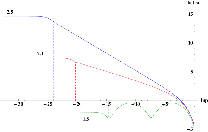
Figure 4.1: log-log plot of $\ln\left|\beta(p)\right|^{2}$ against $\ln p$ at $m=1$, $t_{i}=0$, $t_{f}=10$ and $\omega={\color[rgb]{0,0,1}{2.5}},{\color[rgb]{1,0,0}{2.1}},{\color[rgb]{0,1,0}{1.5}}$

The hyperbolic $\mu>0$ regime is shown in log-log plots of $\ln\left|\beta(p)\right|^{2}$ against $\ln p$ in Figure 4.1 and Figure 4.2. The first figure presents three curves for different values of the expansion parameter while the second uses different $t_{f}$. The values for the other parameters involved are $m=1$ and $t_{i}=0$ with $t_{f}=10$ for the first figure and $\omega=1.0$ for the second. We draw the conclusion that the value of $\left|\beta(p)\right|^{2}$ in the region $q\ll\omega$ (delimited by the dashed line) increases exponentially with both $\omega$ and $t_{f}$ (more precisely, with the expansion time), and is independent of $p$. In subsection 4.2.2 we prove that this value is proportional to $\sinh{\nu\omega\Delta t}$ (4.2.21). The oscillations of the green curve $\omega=1.5$ in the former figure are characteristic to the trigonometric regime (4.2.31), while the declining lines are characteristic to the factor $(2\omega/p)^{2\nu}$ of the hyperbolic regime (4.2.26). From the latter figure we conclude that the middle region $p\ll\omega\ll q$ is independent on the expansion time $t_{f}$, as shown in subsection 4.2.3.

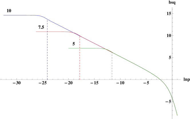
Figure 4.2: log-log plot $t_{f}={\color[rgb]{0,0,1}{10.0}},{\color[rgb]{1,0,0}{7.5}},{\color[rgb]{0,1,0}{5.0}}$

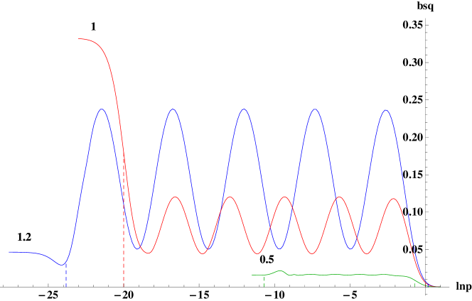
Figure 4.3: lin-log plot $\omega={\color[rgb]{0,0,1}{1.2}},{\color[rgb]{1,0,0}{1.0}},{\color[rgb]{0,1,0}{0.5}}$

Similar figures represent the trigonometric regime, Figure 4.3 for different expansion factors and Figure 4.4 for three different values of $t_{f}$. The parameters used are $m=1$, $t_{i}=0$, $t_{f}=20$ for the former and $\omega=1.0$ for the latter figure. The second figure confirms the result that the middle region is independent of the expansion time. Unlike the hyperbolic case, the value of $\left|\beta(p)\right|^{2}$ in the region $q\ll\omega$ oscillates according to a factor $\sin{\nu\omega\Delta t}$ given in (4.2.21). In the middle region we observ oscillations of constant amplitude about a constant value, which we find to be $m/2\omega\nu(\coth{\pi\nu}-\nu\omega/m)$. Both this value and the amplitude of the oscillations decrease as $\omega$ decreases ($\nu$ increases), the oscillations having a dampening factor proportional to $(\sinh{\pi\nu})^{-1}$ (see (4.2.30)).

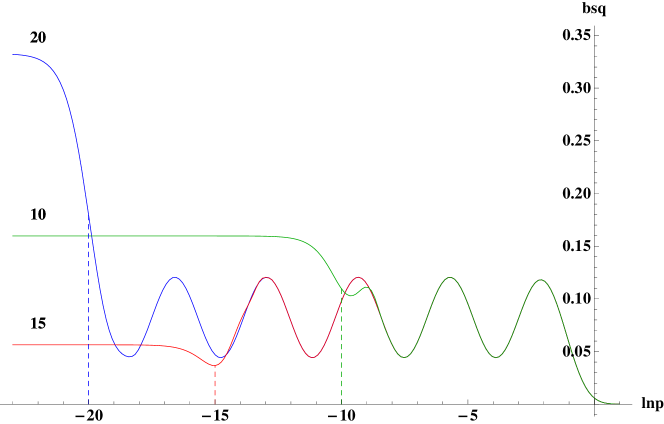
Figure 4.4: lin-log plot $t_{f}={\color[rgb]{0,0,1}{20.0}},{\color[rgb]{1,0,0}{15.0}},{\color[rgb]{0,1,0}{10.0}}$

The fast decline in the ultraviolet region is given by a factor $1/p^{6}$. We illustrate this behaviour in Figure 4.5 where we represent $p^{6}\left|\beta(p)\right|^{2}$ against $\ln p$ for different values of $\omega$, using $m=1,t_{i}=0$ and $t_{f}=10$. The exact solution is checked against the asymptotic value $m^{4}\omega^{2}/16$, and we observe an excellent agreement for sufficiently large $p$.

Figure 4.5: lin-log plot $\omega={\color[rgb]{0,0,1}{1.5}},{\color[rgb]{1,0,0}{1.2}},{\color[rgb]{0,1,0}{0.9}}$

4.2 Asymptotic analysis of the particle density

Before delving into any algebra presented in this chapter, we recommend the reader to carefully read through Appendix A for insight in Hankel functions and their asymptotic forms. We recall some of the notation used throughout this section:

$$M=m+12\omega(\xi-1/6),\qquad\mu^{2}=1/4-M^{2},\qquad\nu=\sqrt{\left|\mu\right|}q,$$

$$Z_{\nu}\left(\frac{p}{\omega}\right)\text{ is given in \eqref{eq:kg_Z_def}},\qquad\beta(p)\text{ is given in \eqref{eq:kg_betaAB}},\qquad Z_{i}(q,p)\text{ defined in \eqref{eq:kg_beta_Z}},$$

$$\Gamma(p,q)=(2\omega/\sqrt{pq})^{\nu}\Gamma(\nu),\qquad\Gamma_{\pm}(p,q)=(2\omega/\sqrt{pq})^{\pm i\nu}\Gamma(\pm i\nu)$$

4.2.1 Large momentum $p\gg\omega$

The first trial of our theory of particle creation is to have a sufficiently fast decay in the ultraviolet region for the particle number density. Since $n_{p}\sim p^{2}\left|\beta(p)\right|^{2}$, we require $\beta(p)$ to decay faster than $p^{3/2}$. Furthermore, the energy density must also go to $0$, therefore we require $\beta(p)$ to decay faster than $p^{2}$.

Although a conformally coupled scalar field satisfies the above requirements, a non-conformally coupled scalar field (and the spinorial field) have a leading term of order $1/p^{2}$, which makes the energy density infinite. Nevertheless, the total number of particles is finite and approaches a constant value for increasing expansion times.

We point out in this subsection that the behaviour of $\left|\beta\right|^{2}$ in the ultraviolet region is, for a conformally coupled scalar field, of order $1/p^{6}$, while for any other coupling it is of order $1/p^{4}$.

First we shall perform a quick analysis on the behaviour of the coefficients $\tilde{A}$ and $\tilde{B}$ defined by (4.1.8) for large values of $p$. In order to estimate their order of magnitude, we will use the zeroth order approximation of the Hankel functions (A.2.3):

$$\left|\tilde{A}(p,t)\right|^{2} \xrightarrow[p\rightarrow\infty]{}\frac{E_{p}}{4p}\left(\left(1+\frac{p}{E_{p}}\right)^{2}+\frac{\omega^{2}}{4E_{p}^{2}}\right),$$ (4.2.1a)

$$\left|\tilde{B}(p,t)\right|^{2} \xrightarrow[p\rightarrow\infty]{}\frac{E_{p}}{4p}\left(\left(1-\frac{p}{E_{p}}\right)^{2}+\frac{\omega^{2}}{4E_{p}^{2}}\right).$$ (4.2.1b)

We see that $A(p,t)$ approaches unity as $p\rightarrow E_{p}$, while $B$ is at most of the order of $p^{-1}$. In order to accurately capture the behaviour of the $\beta$ coefficient for large $p$, we must expand up to order $1/p^{3}$. We shall use Hankel’s expansion given in the appendix (A.2.5). We note that the terms $Z_{i}$ given by (4.1.26) take the following form:

$$Z_{i}(q,p)=\frac{4\omega}{\pi\sqrt{pq}}\left(\cos\frac{q-p}{\omega}C_{i}(q,p)+\sin\frac{q-p}{\omega}S_{i}(q,p)\right).$$ (4.2.2)

For brevity, we shall omit the arguments $(q,p)$ from the functions $C_{i},S_{i}$, which evaluate to:

$$C_{1} =\phantom{-}Q_{q}P_{p}-P_{q}Q_{p}, S_{1} =\phantom{-}P_{q}P_{p}+Q_{q}Q_{p},$$ (4.2.3a)

$$C_{2} =\phantom{-}R_{q}P_{p}+S_{q}Q_{p}, S_{2} =\phantom{-}R_{q}Q_{p}-S_{q}P_{p},$$ (4.2.3b)

$$C_{3} =-P_{q}R_{p}-Q_{q}S_{p}, S_{3} =-P_{q}S_{p}+Q_{q}R_{p},$$ (4.2.3c)

$$C_{4} =-R_{q}S_{p}+S_{q}R_{p}, S_{4} =\phantom{-}R_{q}R_{p}+S_{q}S_{p}.$$ (4.2.3d)

The polynomials $Q,P,R,S$ are given in the appendix by (A.2.5c),(A.2.5d),(A.2.6c),(A.2.6d). We have used the notation $P_{q}=P(\sqrt{\mu},q/\omega)$. Note that the order of the Hankel functions in $Z_{\nu}$ is imaginary for negative $\mu$, in accord with our definition (3.1.13). However, the polynomials are written using $\mu$, and not $\sqrt{\mu}$, thus $C_{i}$ and $S_{i}$ are all real functions. Because the Minkowski energies $E_{p},E_{q}$ can be expanded in a power series as

$$\frac{1}{E_{p}}=\frac{1}{p}\left(1-\frac{m^{2}}{2p^{2}}+\mathcal{O}(p^{-4})\right),$$

it would not be correct to speak of orders of $p$ when analysing $\beta$. Instead, since the terms coming from the Hankel functions are of the form $\omega/p$, we will discuss the coefficient in orders of $\omega$, such that

$$\beta(p)=-\sqrt{\frac{E_{p}E_{q}}{4pq}}e^{-i(E_{q}t_{i}+E_{p}t_{f})}\sum_{n=0}^{\infty}\Omega^{(n)}(q,p)\omega^{n},$$ (4.2.4)

with $\sqrt{\mu}$ being treated as independent of $\omega$. The coefficients $\Omega^{(n)}$, up to order $3$, are given by

$$\Omega^{(0)}(q,p) =\frac{2}{m^{2}}\mathcal{C}(q,p)+\mathcal{O}(p^{-4}),$$ (4.2.5a)

$$\omega\Omega^{(1)}(q,p) =\frac{i\omega m^{2}(4\mu-1)}{16}\left(\frac{1}{p}-\frac{1}{q}\right)\mathcal{C}(q,p)+\mathcal{O}(p^{-5}),$$ (4.2.5b)

$$\omega^{2}\Omega^{(2)}(q,p) =\frac{\omega^{2}(4\mu-1)}{8}\mathcal{C}(q,p)+\mathcal{O}(p^{-4}),$$ (4.2.5c)

$$\omega^{3}\Omega^{(3)}(q,p) =\frac{i\omega^{3}(4\mu-1)^{2}}{64}\left(\frac{1}{p}-\frac{1}{q}\right)\mathcal{C}(q,p)-\frac{i\omega^{3}(4\mu-1)}{8}\times$$

$$\left(\cos\frac{q-p}{\omega}\left(\frac{1}{p^{3}}-\frac{1}{q^{3}}\right)-i\sin\frac{q-p}{\omega}\left(\frac{1}{p^{3}}+\frac{1}{q^{3}}\right)\right)+\mathcal{O}(p^{-5}).$$ (4.2.5d)

The reccurent term is

$$\mathcal{C}(q,p)=\cos\frac{q-p}{\omega}\left(\frac{1}{p^{2}}-\frac{1}{q^{2}}\right)-i\sin\frac{q-p}{\omega}\left(\frac{1}{p^{2}}+\frac{1}{q^{2}}\right).$$ (4.2.5e)

The term $\mu-1/4=-m^{2}/\omega^{2}-12(\xi-1/6)$ magically appears in every term of the expansion, since all higher orders of the polynomials $P,Q,R,S$ share a $4\mu-1$ in their numerator. In the conformally coupled massles case, this term is zero, and thus $\beta$ is 0, as expected (no particle creation for a conformal field).

What is indeed extraordinary is that the leading term in the conformally coupled case $\xi=1/6$ is of order $p^{-3}$, while in any other coupling (including the minimal coupling $\xi=0$), it is of order $p^{-2}$:

$$\beta(p)=\omega^{2}\frac{E_{p}E_{q}}{4pq}e^{-i(E_{q}t_{i}+E_{p}t_{f})}\bigg{\{}12(\xi-1/6)(\mathcal{C}(q,p)+\mathcal{O}(p^{-3}))-\\ i\omega\left(\frac{m^{2}}{\omega^{2}}+12(\xi-1/6)\right)\left(\cos\frac{q-p}{\omega}\left(\frac{1}{p^{3}}-\frac{1}{q^{3}}\right)-i\sin\frac{q-p}{\omega}\left(\frac{1}{p^{3}}+\frac{1}{q^{3}}\right)\right)\\ +\mathcal{O}(p^{-4})\bigg{\}}.$$ (4.2.6)

The square of this coefficient, in the minimally coupled case, is

$$\left|\beta(p)\right|^{2}_{\xi=0}\xrightarrow[p\gg\omega]{}\frac{\omega^{4}}{2p^{4}}e^{-2\omega(t_{f}-t_{i})}\left(\cosh{2\omega\Delta t}-\cos\frac{2(q-p)}{\omega}\right).$$ (4.2.7)

In the conformally coupled case we have

$$\left|\beta(p)\right|^{2}_{\xi=1/6}\xrightarrow[p\gg\omega]{}\frac{m^{4}\omega^{2}}{8p^{6}}e^{-3\omega(t_{f}-t_{i})}\left(\cosh{3\omega\Delta t}-\cos\frac{2(q-p)}{\omega}\right).$$ (4.2.8)

With $\Delta t=t_{f}-t_{i}$ being the total time of expansion. In the limit of large expansion times, we can neglect the cosine term while the hyperbolic cosine can be replaced by $1/2$:

$$\left|\beta(p)\right|^{2}_{\xi=0} \xrightarrow[t_{f}\gg t_{i}]{}\frac{\omega^{4}}{4p^{4}},$$ (4.2.9)

$$\left|\beta(p)\right|^{2}_{\xi=1/6} \xrightarrow[t_{f}\gg t_{i}]{}\frac{m^{4}\omega^{2}}{16p^{6}}.$$ (4.2.10)

For future reference we shall denote the coefficient of the conformally coupled scalar field by

$$\left|\beta(p)\right|^{2}_{l}\equiv\frac{m^{4}\omega^{2}}{16p^{6}}.$$ (4.2.11)

A short note about different junction conditions: if we choose not to impose continuity on $e^{\omega t}f_{{\boldsymbol{p}}}^{\rm dS}$, but on a different function $e^{\omega t(1-\alpha)}f_{{\boldsymbol{p}}}^{\rm dS}$, then the $\beta$ coefficient will have a leading term of order $p^{-1}$,

$$\Omega^{(1)}(q,p)=i\alpha\omega\left(\cos{\frac{q-p}{\omega}}\left(\frac{1}{p}-\frac{1}{q}\right)-i\sin\frac{q-p}{\omega}\left(\frac{1}{p}+\frac{1}{q}\right)\right),$$ (4.2.12)

which has the effect of producing an infinite number of particles per unit volume of space, since the spectral density of particles approaches a constant in the ultraviolet region:

$$n_{p}(x)\xrightarrow[t_{f}\gg t_{i}]{}\frac{\alpha^{2}\omega^{2}}{8\pi^{2}}.$$ (4.2.13)

We note that this result is independent of the choice of the coupling $\xi$ with the gravitational field.

4.2.2 Low momentum $q\ll\omega$

In this section we point out that the particle number density approaches a constant value in the infrared region, meaning low energy modes are equally populated by the expansion of space.

In order to investigate the infrared asymptotic behaviour of $\beta$ we need to consider the approximation $q\ll\omega$. We will approximate the Hankel functions in (4.1.26) with their asymptotic forms for small values of the argument given by (A.2.1), and their derivatives with (A.2.2). Note that since the order of the functions is $\sqrt{\mu}$ with an unbounded $\mu$, we cannot restrict ourselves to the term $2/z$ since there is a significant contribution comming from $z/2$ if the power $\sqrt{\mu}$ is not real.

In this approximation, the real terms $Z_{i}$ given by (4.1.26) read

$$Z_{1} =\phantom{-}\frac{4}{\pi\sqrt{\mu}}\sinh{\sqrt{\mu}\omega\Delta t}, Z_{2} =\phantom{-}\frac{4\omega}{q\pi}\cosh{\sqrt{\mu}\omega\Delta t},$$ (4.2.14a)

$$Z_{4} =-\frac{4\sqrt{\mu}\omega^{2}}{\pi pq}\sinh{\sqrt{\mu}\omega\Delta t}, Z_{3} =-\frac{4\omega}{p\pi}\cosh{\sqrt{\mu}\omega\Delta t}.$$ (4.2.14b)

With this we evaluate the $\beta$ coefficient to

$$\beta(p)\xrightarrow[q\ll\omega]{}-\frac{\sinh{\sqrt{\mu}\omega\Delta t}}{2\sqrt{\mu}}e^{-i(E_{q}t_{i}+E_{p}t_{f})}\times\\ \left\{\frac{1}{2}\left(\sqrt{\frac{E_{q}}{E_{p}}}+\sqrt{\frac{E_{p}}{E_{q}}}\right)+\sqrt{\mu}\coth{\sqrt{\mu}\omega\Delta t}\left(\sqrt{\frac{E_{p}}{E_{q}}}-\sqrt{\frac{E_{q}}{E_{p}}}\right)+\right.\\ \left.i\frac{\sqrt{E_{p}E_{q}}}{\omega}\left(-1+\frac{m^{2}}{E_{p}E_{q}}+\frac{12\omega^{2}}{E_{p}E_{q}}\left(\xi-1/6\right)\right)\right\}.$$ (4.2.15)

Since we have not retained any powers of $p$ in the above approximation, we shall replace $E_{p}$ and $E_{q}$ with $m$. Higher order terms will not contribute correctly, because we have suppressed potentially balancing terms. Using $1/4-\mu=m^{2}/\omega^{2}+12(\xi-1/6)$ we arrive at the following form for the $\beta$ coefficient:

$$\beta(p)\xrightarrow[q\ll\omega]{}-\frac{\sinh{\sqrt{\mu}\omega\Delta t}}{2\sqrt{\mu}}e^{-i(E_{q}t_{i}+E_{p}t_{f})}\left(1-12i\left(\xi-1/6\right)\right).$$ (4.2.16)

Again, in the conformally coupled case the production of particles is at a minimum. We give the two values for the square of $\beta$ in the minimally and conformally coupled cases:

$$\left|\beta(p)\right|^{2}_{\xi=0} \xrightarrow[q\ll\omega]{}\frac{5\sinh^{2}{\sqrt{\mu}\omega\Delta t}}{16\mu},$$ (4.2.17)

$$\left|\beta(p)\right|^{2}_{\xi=1/6} \xrightarrow[q\ll\omega]{}\frac{\sinh^{2}{\sqrt{\mu}\omega\Delta t}}{4\mu}.$$ (4.2.18)

We identify two different regimes: if $\mu=1/4-m^{2}/\omega^{2}-12\xi+2$ is pozitive (small mass or large expansion rate), $\beta$ increases exponentially as the expansion rate increases. In the case $\mu<0$, the hyperbolic functions turn into trigonometric ones, and $\left|\beta(p)\right|^{2}$ oscillates as the expansion time increases. The massless case is not correctly captured by this approximation, since we have replaced $E_{p}$ and $E_{q}$ by $m$, and neglected the difference $E_{p}-E_{q}$. If we neglect terms of order $p$ in (4.2.15) we obtain

$$\beta(p)_{\begin{subarray}{c}\xi=1/6\\ m=0\end{subarray}}\xrightarrow[q\ll\omega]{}0.$$ (4.2.19)

The equality is not exact (as shown in subsection 4.1.3) because of an inaccurate treatment of higher order terms in the approximation used. We note that if the massless field is not conformally coupled, $\beta(p)$ is infinite for $p\rightarrow 0$ because of the coefficient of $\xi-1/6$:

$$\beta(p)\xrightarrow[\begin{subarray}{c}q\ll\omega\\ m=0\end{subarray}]{}-\frac{\sinh{\sqrt{\mu}\omega\Delta t}}{2\sqrt{\mu}}e^{-i(E_{q}t_{i}+E_{p}t_{f})}\frac{12i\omega}{\sqrt{qp}}\left(\xi-1/6\right)+\mathcal{O}(p^{0}).$$ (4.2.20)

We denote the asymptotic form of $\left|\beta(p)\right|^{2}$ in the conformally coupled case by

$$\left|\beta(p)\right|^{2}_{s}=\frac{\sinh^{2}{\sqrt{\mu}\omega\Delta t}}{4\mu}.$$ (4.2.21)

4.2.3 Middle region $p\ll\omega\ll q$

The ubiquitous thermal spectrum of the particle density created by the de Sitter space is not recovered. Not only does it not emerge for large $\omega$, but even when $\omega$ is sufficiently small, there is a polynomial correction to the thermal Bose-Einstein distribution, which is dominant for large masses (small expansion parameter).

In the middle region we shall use the small argument approximation for the Hankel functions of argument $p/\omega$, and the large argument approximation for those of $q/\omega$. We shall use first order approximations, and we shall substitute directly in the expressions for the $A,B$ coefficients (4.1.6), because the asymmetry of the approximations for $p$ and $q$ makes the use of the general formula for $\beta$ (4.1.24) unnecessarily cumbersome.

In subsection 4.2.1 we have investigated the behaviour of the coefficient $A$ and $B$ for large values of the argument, and have concluded that the $B(q,t)$ coefficient drops like $1/q$ (4.2.1). Since the domain of interest is for increasing values of $p$ (and $q$), we shall not delve on accurate representations of the small momentum domain, and instead use the approximation $B(q,t)\simeq 0$. Therefore $\beta$ reduces to

$$\beta(p)\xrightarrow[p\ll\omega\ll q]{}\tilde{A}(q,t_{i})\tilde{B}(p,t_{f}).$$

Substituting (4.2.1a) for $\tilde{A}(q,t_{i})$, and computing $\tilde{B}(p,t_{f})$ by substituting (A.2.1) and (A.2.2) for the Hankel functions and their derivatives, we arrive at

$$\beta(p)\xrightarrow[p\ll\omega\ll q]{}-\sqrt{\frac{\pi E_{p}E_{q}}{8\omega q}}e^{-i(E_{q}t_{i}+E_{p}t_{f})}e^{-i\frac{q}{\omega}+\frac{i\pi\sqrt{\mu}}{2}+\frac{i\pi}{4}}\left\{\left(\frac{2\omega}{p}\right)^{\sqrt{\mu}}\frac{\Gamma(\sqrt{\mu})}{i\pi}\left(1-\frac{i\nu\omega}{E_{p}}+\frac{i\omega}{2E_{p}}\right)+\right.\\ \left.\left(\frac{p}{2\omega}\right)^{\sqrt{\mu}}\frac{1+i\cot{\pi\sqrt{\mu}}}{\sqrt{\mu}\Gamma(\sqrt{\mu})}\left(1+\frac{i\nu\omega}{E_{p}}+\frac{i\omega}{2E_{p}}\right)\right\}.$$ (4.2.22)

In order to compute $\left|\beta(p)\right|^{2}$ we must consider separately the cases $\mu>0$ and $\mu<0$. If $\mu>0$ (thus $\sqrt{\mu}$ is real), we have $\sqrt{\mu}=\nu$ and the dominant term is $1/p^{\nu}$. Although we can discard the higher order terms for the purpose of this analysis, they are not negligible near the region $p\sim\omega$, important for the analysis of the total number of created particles. Moreover, the free term uncovers a thermal factor corresponding to an imaginary energy. We write the square of (4.2.22) in this approximation:

$$\left|\beta(p)\right|^{2}_{\mu>0}\xrightarrow[p\ll\omega\ll q]{}\frac{E_{p}E_{q}}{2\omega\nu q}\left(\cot{\pi\nu}\left(\frac{1}{2}+\frac{M^{2}}{2E_{p}^{2}}\right)+\frac{\nu\omega}{E_{p}}\right)+\frac{\omega E_{q}}{8\pi E_{p}q}\Bigg{\{}\\ \Gamma(p,p)\left(\frac{E_{p}^{2}}{\omega^{2}}+\left(\frac{1}{2}-\nu\right)^{2}\right)+\frac{\pi^{2}}{\nu^{2}\sin^{2}{\pi\nu}\Gamma^{2}(p,p)}\left(\frac{E_{p}^{2}}{\omega^{2}}+\left(\frac{1}{2}+\nu\right)^{2}\right)\Bigg{\}}.$$ (4.2.23)

We have used the notation

$$\Gamma(q,p)=\left(\frac{2\omega}{\sqrt{qp}}\right)^{\nu}\Gamma(\nu).$$ (4.2.24)

In the region where $E_{p}\sim m$, and for a conformally coupled scalar field ($M=m$), the first term takes the form

$$-\frac{m}{2\omega\nu}\left(\cot{\pi\nu}+\frac{\nu\omega}{m}\right).$$

Assuming that a Taylor series expansion for $\nu$ about $\omega/m=0$ makes sens (which it doesn’t, since the case $\mu>0$ implies $m/\omega<1/2$), and ignoring the apparent complex (i.e. non-real) nature of the result, this term gives a thermal factor (plus a polynomial correction):

$$\frac{1}{e^{2\pi i\nu}-1}+\frac{\omega^{2}}{16m^{2}}-\frac{\omega^{2}}{8m^{2}}\frac{1}{e^{2\pi i\nu}-1}+\mathcal{O}\left(\frac{\omega^{4}}{m^{4}}\right).$$ (4.2.25)

We note that this factor contributes significant corrections for $\nu\lesssim 1/4$, and in the region $p\sim\omega$, therefore we shall include it in the final form:

$$\left|\beta(p)\right|^{2}_{\begin{subarray}{c}\xi=1/6\\ \mu>0\end{subarray}}\xrightarrow[p\ll\omega\ll q]{}\left|\beta(p)\right|^{2}_{m}=-\frac{m}{2\omega\nu}\left(\cot{\pi\nu}+\frac{\omega\nu}{m}\right)+\frac{\omega}{8\pi m}\Bigg{\{}\\ \Gamma^{2}(p,p)\left(\frac{m^{2}}{\omega^{2}}+\left(\frac{1}{2}-\nu\right)^{2}\right)+\frac{\pi^{2}}{\nu^{2}\sin^{2}{\pi\nu}\Gamma^{2}(p,p)}\left(\frac{m^{2}}{\omega^{2}}+\left(\frac{1}{2}+\nu\right)^{2}\right)\Bigg{\}}.$$ (4.2.26)

Let us turn to the case $\mu<0$, $\sqrt{\mu}=i\nu$. In the square of $\beta$ we shall encounter an approximately constat term which will give the thermal character about which a second term oscillates, whose amplitude decreases as the expansion factor decreases, or the mass increases. Using

$$\left|\Gamma(i\nu)\right|^{2}=\frac{\pi}{\nu\sinh{\pi\nu}},$$

the constant term writes

$$T_{c}=\frac{E_{p}}{4\nu\omega}\left(\coth{\pi\nu}\left(1+\frac{M^{2}}{E_{p}^{2}}\right)-\frac{2\nu\omega}{E_{p}}+\dots\right).$$

while the oscillating term is

$$T_{o}=\frac{E_{p}}{8\pi\omega}\left\{\left(1-\frac{M^{2}}{E_{p}^{2}}+\frac{\omega^{2}}{2E_{p}^{2}}\right)\left(\Gamma_{+}^{2}(p,p)+\Gamma_{-}^{2}(p,p)\right)-\frac{i\omega^{2}\nu}{E_{p}^{2}}\left(\Gamma_{+}^{2}(p,p)-\Gamma_{-}^{2}(p,p)\right)\right\}.$$

We have used the notation

$$\Gamma_{\pm}(p,q)=\left(\frac{2\omega}{\sqrt{pq}}\right)^{\pm i\nu}\Gamma(\pm i\nu)\,,\,\Gamma_{+}^{*}(p,q)=\Gamma_{-}(p,q)\,,\,\left|\Gamma_{+}(p,q)\right|^{2}=\frac{\pi}{\nu\sinh{\pi\nu}}.$$ (4.2.27)

In the conformally coupled case, we make the approximation $E_{p}\simeq M=m$, and obtain:

$$T_{c} =\frac{m}{2\nu\omega}\left(\coth{\pi\nu}-\frac{\nu\omega}{m}\right),$$

$$T_{o} =\frac{\omega}{16\pi m}\left\{\left(\Gamma_{+}^{2}(p,p)+\Gamma_{-}^{2}(p,p)\right)-2i\nu\left(\Gamma_{+}^{2}(p,p)-\Gamma_{-}^{2}(p,p)\right)\right\}.$$

For large masses (or small expansion factors), we can obtain a term resembling the Bose-Einstein distribution function, by expanding $\nu$ in a power series about $\omega/m=0$:

$$T_{c}=\frac{1}{e^{2\pi\nu}-1}+\frac{\omega^{2}}{16m^{2}}+\mathcal{O}\left(\frac{\omega^{4}}{m^{4}}\right).$$ (4.2.28)

However, this distribution does not have the characteristic of a Bose-Einstein decaying exponential, since for large $m$ the polynomial term is dominant.

In order to determine the amplitude of the oscillatory term $T_{o}$ we define $\theta_{\Gamma}$ such that

$$\Gamma_{\pm}(p,p)^{2}=\frac{\pi}{\nu\sinh{\pi\nu}}e^{2i\theta_{\Gamma}},$$ (4.2.29)

since $\left|\Gamma_{+}(p,p)\right|^{2}=\pi/\nu\sinh{\pi\nu}$. In this notation, the oscillatory term writes

$$T_{o}=\frac{1}{4\nu\sinh{\pi\nu}}\left(\frac{1}{\sqrt{1+4\nu^{2}}}\cos{2\theta_{\Gamma}}+\frac{2\nu}{\sqrt{1+4\nu^{2}}}\sin{2\theta_{\Gamma}}\right).$$ (4.2.30)

This term exponentially approaches $0$ with increasing $\nu$, but becomes large at $\nu\rightarrow 0$ (the result is not accurate for $\nu=0$ since the expansion we used for low arguments is not valid for Hankel functions of order $0$). We shall keep the oscillatory term in the final form of $\left|\beta(p)\right|^{2}$:

$$\qquad\left|\beta(p)\right|^{2}_{\begin{subarray}{c}\xi=1/6\\ \mu<0\end{subarray}}\xrightarrow[p\ll\omega\ll q]{}\left|\beta(p)\right|^{2}_{m}=\frac{m}{2\omega\nu}\left(\coth{\pi\nu}-\frac{\nu\omega}{m}\right)+\\ \frac{\omega}{8\pi m}\left\{\frac{1}{2}\left(\Gamma_{+}^{2}(p,p)+\Gamma_{-}^{2}(p,p)\right)-i\nu\left(\Gamma_{+}^{2}(p,p)-\Gamma_{-}^{2}(p,p)\right)\right\}.\qquad$$ (4.2.31)

The behaviour of $\left|\beta(p)\right|^{2}$ in the middle region $p\ll\omega\ll q$ is unrelated to $t_{i},t_{f}$.

4.2.4 The number of created particles

The asymptotic analysis of the previous section enables us to approximate $\left|\beta(p)\right|^{2}$ to a good degree of accuracy on the entire domain $p\in[0,\infty)$. However, even though the approximation approaches the form of the exact solution, the function $p^{2}\left|\beta(p)\right|^{2}$ is notably different because the relevant region of integration is near $p\sim\omega$, where none of the above approximations are valid.

The difficult part in obtaining integrals of $\left|\beta(p)\right|^{2}$ is choosing the right ranges for the asymptotic forms. The delicate areas are the borders of the asymptotic regions, namely $q\sim\omega$ and $p\sim\omega$. The solution is to define

$$\left|\beta(p)\right|^{2}_{as}=\begin{cases}\left|\beta(p)\right|^{2}_{s}&q<\omega,\\ \left|\beta(p)\right|^{2}_{m}&\omega<q\text{ and }p<p_{\nu},\\ \left|\beta(p)\right|^{2}_{l}&p>p_{\nu}.\end{cases}$$ (4.2.32)

The choice for the first branch is natural, since $\left|\beta(p)\right|^{2}_{s}$ is constant (see (4.2.21)), and $\left|\beta(p)\right|^{2}_{m}$ is either decreasing (in the hyperbolic case, see (4.2.26)) or oscillating about a constant value (in the trigonometric case, see (4.2.31)), therefore there is no risc of having the asymptotic form increase too much. Inevitably, there will be a region where this approximation is not accurate. On the other hand, the choice of the second point $p_{\nu}$ is not straightforward. Although the asymptotic form for large arguments $\left|\beta(p)\right|^{2}_{l}$ given by (4.2.11) is monotonic and decreasing, it approaches infinity as $p$ approaches $0$, while $\left|\beta(p)\right|^{2}_{m}$ goes to large values when $p>\omega$. In order to solve this difficulty we choose $p_{\nu}$ such that

$$\left|\beta(p)\right|^{2}_{m}(p_{\nu})=\left|\beta(p)\right|^{2}_{l}(p_{\nu}).$$ (4.2.33)

We have to analyze both the hyperbolic and the trigonometric case. Unfortunately, the complex behaviour of $\left|\beta(p)\right|^{2}_{m}$ outside the scope of their definition ($p\sim\omega$) makes the equation (4.2.33) unsolvable. In the hyperbolic case we choose, by trial and error, $p_{\nu}=\sqrt{2m\omega/3}$. For the trigonometric case we consider the constant term minus the amplitude of the oscillations (since $\left|\beta(p)\right|^{2}$ is decreasing below this value at a fast rate), and arrive at

$$p_{\nu}=\begin{cases}\sqrt{2m\omega/3}&\mu>0,\\ {\displaystyle\sqrt{\frac{m\omega}{2}}\nu^{1/6}(\coth{\pi\nu}-\frac{\omega\nu}{m}-\frac{\omega}{2m\sinh{\pi\nu}})^{-1/6}}&\mu<0.\end{cases}$$ (4.2.34)

We write the particle number space density as the integral of the particle number density with magnitude $p$ given in Equation 4.1.18, which we split according to the piecewise definition of our asymptotic form (4.2.32):

$$n(\boldsymbol{x})=\frac{1}{2\pi^{2}}\left(I_{s}+I_{m}+I_{l}\right),$$

$$I_{s}=\int_{0}^{q=\omega}dp\,p^{2}\left|\beta(p)\right|^{2}_{s},\qquad I_{m}=\int_{q=\omega}^{p=p_{\nu}}dp\,p^{2}\left|\beta(p)\right|^{2}_{m},\qquad I_{l}=\int_{p_{\nu}}^{\infty}p^{2}\left|\beta(p)\right|^{2}_{l}.$$

We have used $q=\omega$ as a shorthand for $p=\omega e^{-\omega\Delta t}$. $I_{s}$ and $I_{l}$ evaluate to

$$I_{s}=\frac{\sinh^{2}{\sqrt{\mu}\omega\Delta t}}{12\mu}\omega^{3}e^{-3\omega\Delta t},\qquad I_{l}=\frac{m^{4}\omega^{2}}{48}\frac{1}{p_{\nu}^{3}}.$$ (4.2.35)

In the middle region we need to integrate $\Gamma^{\pm 2}(p,p)$ (defined by (4.2.24) for the hyperbolic case) and $\Gamma^{2}_{\pm}(p,p)$ (defined by (4.2.27) for the trigonometric case), for which we find the results:

$$\int_{q=\omega}^{p=p_{\nu}}dp\,p^{2}\Gamma^{\pm 2}(p,p) =\frac{1}{3\mp 2\nu}\left(p_{\nu}^{3}\Gamma^{\pm 2}(p_{\nu},p_{\nu})-\omega^{3}e^{-3\omega\Delta t}\Gamma^{\pm 2}(\omega e^{-\omega\Delta t},\omega e^{-\omega\Delta t})\right),$$

$$\int_{q=\omega}^{p=p_{\nu}}dp\,p^{2}\Gamma^{2}_{\pm}(p,p) =\frac{1}{3\mp 2i\nu}\left(p_{\nu}^{3}\Gamma^{2}_{\pm}(p_{\nu},p_{\nu})-\omega^{3}e^{-3\omega\Delta t}\Gamma^{2}_{\pm}(\omega e^{-\omega\Delta t},\omega e^{-\omega\Delta t})\right).$$

After neglecting the terms $e^{-\omega\Delta t}$, we arrive at

$$n^{\text{hyp}}(\boldsymbol{x})=\frac{1}{2\pi^{2}}\Bigg{\{}\frac{m^{4}\omega^{2}}{48p_{\nu}^{3}}-\frac{mp_{\nu}^{3}}{6\omega\nu}\left(\cot{\pi\nu+\omega\nu/m}\right)+\\ \frac{\omega p_{\nu}^{3}}{8\pi m}\left[\frac{\Gamma^{2}(p_{\nu},p_{\nu})}{3-2\nu}\left(m^{2}/\omega^{2}+\left(1/2-\nu\right)^{2}\right)+\frac{\pi^{2}}{\nu^{2}\sin^{2}{\pi\nu}}\frac{\Gamma^{-2}(p_{\nu},p_{\nu})}{3+2\nu}\left(m^{2}/\omega^{2}+\left(1/2+\nu\right)^{2}\right)\right]\Bigg{\}},\\ n^{\text{trig}}(\boldsymbol{x})=\frac{1}{2\pi^{2}}\Bigg{\{}\frac{m^{4}\omega^{2}}{48p_{\nu}^{3}}+\frac{mp_{\nu}^{3}}{6\omega\nu}\left(\coth{\pi\nu}-\omega\nu/m\right)+\\ \frac{\omega p_{\nu}^{3}}{8\pi m}\left[\Gamma^{2}_{+}(p_{\nu},p_{\nu})\frac{1/2-i\nu}{3-2i\nu}+\Gamma^{2}_{-}(p_{\nu},p_{\nu})\frac{1/2+i\nu}{3+2i\nu}\right]\Bigg{\}}.$$ (4.2.36)

We conclude that if the time interval $\Delta t=t_{f}-t_{i}$ is sufficiently large the particle number density approaches a constant value. In order to understand the dependence on $m$ and $\omega$, which is highly dependent on the choice of $p_{\nu}$, we take the extreme cases $m/\omega\rightarrow 0$ (hyperbolic regime), and $\omega/m\rightarrow 0$ (trigonometric regime).

In the first case we can approximate $\nu=1/2$ and get

$$n^{\text{hyp}}(\boldsymbol{x})\xrightarrow[m/\omega\rightarrow 0]{}\frac{1}{2\pi^{2}}\left\{\frac{m\omega^{2}}{36}-\frac{\sqrt{6}}{27}(m\omega)^{3/2}+\frac{\omega m^{2}}{12}+\frac{\sqrt{6}}{64}m^{2}(m\omega)^{1/2}\right\}.$$ (4.2.37)

The leading term is quadratic in $\omega^{2}$, but it becomes dominant only for large $\omega/m$. Since $m$ appears in each of the above terms, we conclude that there is no particle production in the masless case:

$$n^{\text{hyp}}(\boldsymbol{x})\xrightarrow[m=0]{}0.$$ (4.2.38)

The asymptotic $m$ dependence can be investigated by letting $\omega/m\rightarrow 0$ (trigonometric regime). In this limit we can use:

$$\nu\simeq\frac{m}{\omega}\left(1-\frac{\omega^{2}}{8m^{2}}\right),\qquad\frac{1}{\nu}\simeq\frac{\omega}{m}\left(1+\frac{\omega^{2}}{8m^{2}}\right),\qquad\coth{\pi\nu}\simeq 1,$$

$$\sinh{\pi\nu}\simeq e^{\pi\nu},\qquad\Gamma_{\pm}^{2}(p_{\nu},p_{\nu})=\frac{1}{\nu\sinh{\pi\nu}}e^{\pm 2i\theta_{\Gamma}}\simeq 0$$

$$p_{\nu}\simeq\sqrt{\frac{m\omega}{2}}(1/\nu-\omega/m)^{-1/6}\simeq m$$

With which we get

$$n^{\text{trig}}(\boldsymbol{x})\xrightarrow[\omega/m\rightarrow 0]{}\frac{m\omega^{2}}{48\pi^{2}}.$$ (4.2.39)

This dependency is similar to that for large $\omega/m$, up to a factor $3/2$. We emphasize again that these results depend strongly on the choice of $p_{\nu}$, which we have chosen rather empirically in the hyperbolic case. This term becomes quickly dominant and reproduces remarkably well the exact result. From the above formula we can conclude that there is no particle production for $\omega=0$:

$$n^{\text{trig}}(\boldsymbol{x})\xrightarrow[\omega=0]{}0.$$ (4.2.40)

4.2.5 Graphical comparison to the exact solution

The piecewise definition of the asymptotic form of $\left|\beta(p)\right|^{2}$ (4.2.32) can be used to approximate $\left|\beta(p)\right|^{2}$ on the entire domain $p\in[0,\infty)$. This approximate form can be used for the computation of the particle number density $n(\boldsymbol{x})$. However, we expect some differences to occur because of the inaccuracy of the approximation near the delimiters $q\sim\omega$ and $p\sim\omega$.

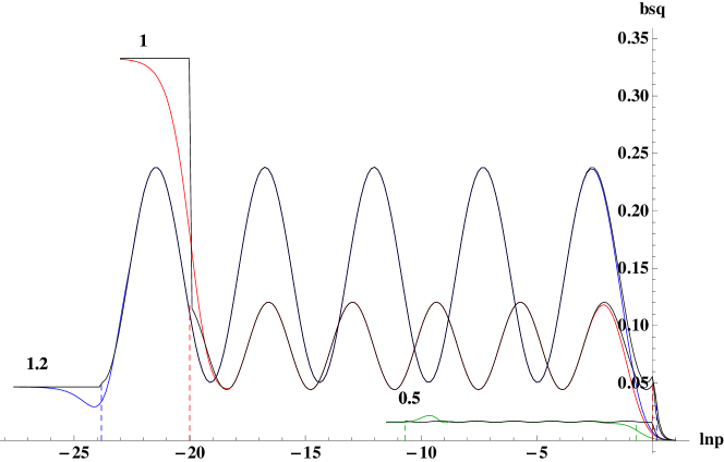
Figure 4.6: lin-log plot $\omega={\color[rgb]{0,0,1}{1.2}},{\color[rgb]{1,0,0}{1.0}},{\color[rgb]{0,1,0}{0.5}}$

The overlap between the analytical solution and the corresponding asymptotic forms is given in Figure 4.6 (compare to Figure 4.3) and Figure 4.7(compare to Figure 4.1). The most striking disagreement is near $q\lesssim\omega$ (before the dashed lines), where the asymptotic form for low arguments is no longer accurate. There is another disagreement near $p\sim\omega$, where the asymptotic forms corresponding to large $p$ and small $p$ respectivelly start to increase (the former like $1/p^{6}$), while $\left|\beta(p)\right|^{2}$ enters a decline.

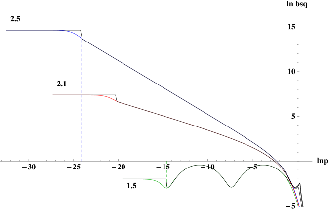
Figure 4.7: log-log plot $\omega={\color[rgb]{0,0,1}{2.5}},{\color[rgb]{1,0,0}{2.1}},{\color[rgb]{0,1,0}{1.5}}$

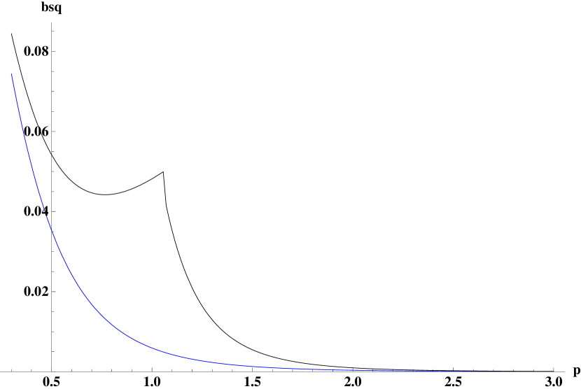
Figure 4.8: lin-lin plot $m=\omega=1$

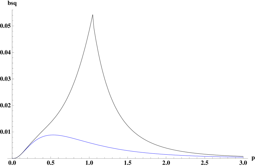
Figure 4.9: lin-lin plot of $p^{2}\left|\beta(p)\right|^{2}$ against $p$ for $m=\omega=1$

The inaccuracy of the asymptotic forms is depicted in Figure 4.9 at the level of $\left|\beta(p)\right|^{2}$ and in Figure 4.9 at the level of $p^{2}\left|\beta(p)\right|^{2}$.

The resulting total number of particles,

$$n(\boldsymbol{x})=\int_{0}^{\infty}\frac{p^{2}}{2\pi^{2}}\left|\beta(p)\right|^{2},$$

is a function of $m$ and $\omega$, irrespective of the expansion time (in the limit $q\gg p$). Our asymptotic analysis provides a good approximation of this number, up to an almost constant proportionality factor caused by the difference between the exact solution and the asymptotic form depicted in Figure 4.9. This can be seen by the plot in Figure 4.10, where we show the result of the numerical integration $\ln n(\boldsymbol{x})$ as a function of $m$, at $t_{i}=0$, $t_{f}=10$ and $\omega=1.0$, compared with our asymptotic form, from which we approximate this factor by $3.5$. In subsequent plots we shall divide the asymptotic results by this factor. There is a very small discontinuity occuring at $\mu=0$ because of the discontinuity in $p_{\nu}$ and because of the piecewise definition we have employed.

Figure 4.10: $\ln n(\boldsymbol{x})$ as a function of the particle mass $m$ at $\omega=1$

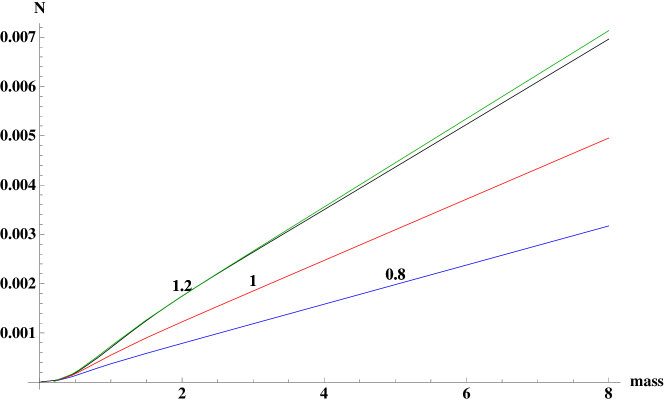
Figure 4.11: $n(\boldsymbol{x})$ as a function of the particle mass $m$ for $\omega={\color[rgb]{0,0,1}{0.8}},{\color[rgb]{1,0,0}{1.0}},{\color[rgb]{0,1,0}{1.2}}$ (asymptotic solution is divided by $3.5$)

It is remarkable that we obtain a very good agreement with the exact solution. In Figure 4.11 we show the particle number density $n(\boldsymbol{x})$ as a function of the particle mass for different $\omega$, and in Figure 4.12 we plot against $\omega$ for different $m$. The other parameters are $t_{i}=0$ and $t_{f}=10$.

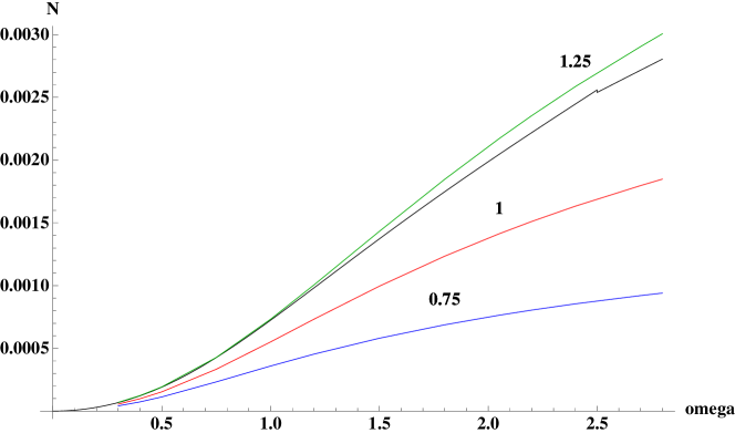
Figure 4.12: $n(\boldsymbol{x})$ as a function of the expansion factor $\omega$ for $m={\color[rgb]{0,0,1}{0.75}},{\color[rgb]{1,0,0}{1.00}},{\color[rgb]{0,1,0}{1.25}}$ (asymptotic solution is divided by $3.5$)

Finally, the energy density $\mathcal{E}(\boldsymbol{x})$ is shown in Figure 4.14 as a function of $m$ and in Figure 4.14 with respect to $\omega$.

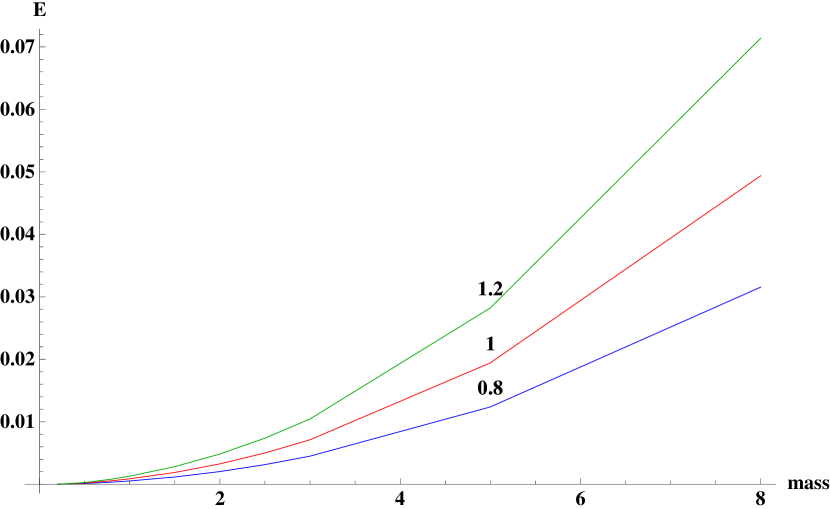
Figure 4.13: $\mathcal{E}(\boldsymbol{x})$ as a function of the mass $m$ for $\omega={\color[rgb]{0,0,1}{0.8}},{\color[rgb]{1,0,0}{1.0}},{\color[rgb]{0,1,0}{1.2}}$

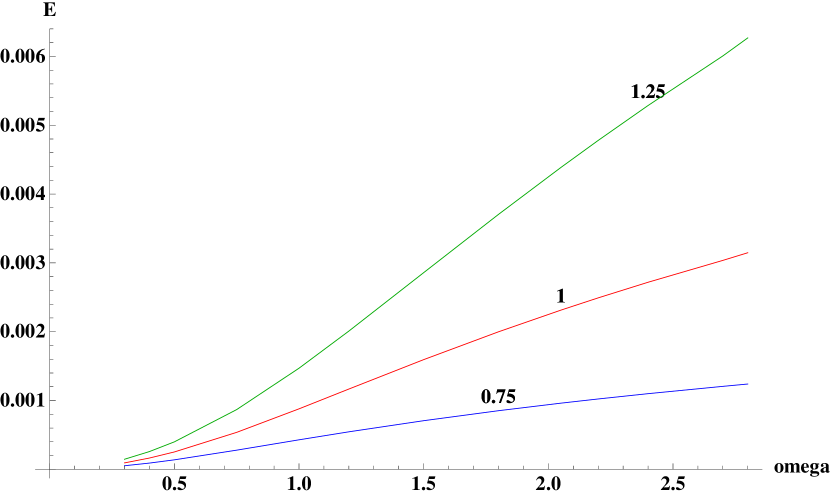
Figure 4.14: $\mathcal{E}(\boldsymbol{x})$ as a function of the expansion factor $\omega$ for $m={\color[rgb]{0,0,1}{0.75}},{\color[rgb]{1,0,0}{1.00}},{\color[rgb]{0,1,0}{1.25}}$

We conclude that the particle number density does not depend on the expansion time $t_{f}-t_{i}$ as long as the latter is sufficiently large ($\omega\Delta t>1$). There is linear increase with the particle mass (4.2.39), and a quadratic increase with the expansion factor (4.2.37). The energy density $\mathcal{E}(\boldsymbol{x})$ exhibits a similar increase with the expansion factor, but the $m$ dependence is more pronounced, and looks quadratic.

Chapter 5 Creation of spinorial particles

5.1 Bogoliubov coefficients

We follow the procedure of section 4.1 for the continuation of Minkowski modes from the out (in) region through the de Sitter expansion phase in the in (out) region.

5.1.1 de Sitter in and out modes

The Dirac equation, being a first order differential equation, requires only one initial value equation to completely determine a mode. However, since the modes are spinors, there are actually two independent equations, one for the upper spinor and one for the lower one. The junction equation is

$$U^{\rm out}_{{\boldsymbol{p}},\lambda}(t_{f},\boldsymbol{x})=U^{\text{M}_{f}}_{{\boldsymbol{p}},\lambda}(t_{f},\boldsymbol{x}),$$ (5.1.1)

with $U^{\rm out}$ given as a linear combination of de Sitter solutions, with the coefficients determined by

$$A(p,t_{f})U_{{\boldsymbol{p}}_{f},\lambda}^{\textrm{dS}}(t_{f},\boldsymbol{x})+B(p,t_{f})V_{-{\boldsymbol{p}}_{f},\lambda}^{\textrm{dS}}(t_{f},\boldsymbol{x})=U_{{\boldsymbol{p}},\lambda}^{\textrm{$\text{M}_{f}$}}(t_{f},\boldsymbol{x}).$$ (5.1.2)

The de Sitter spinors can be read from (3.2.20) and the Minkowski ones from (3.3.8). Using the connection between the Pauli spinors (B.3.3), we can cast the above relation in matrix form:

$$\qquad\begin{pmatrix}ie^{\pi k/2}{H^{(1)}_{\nu_{-}}}\left(\frac{p}{\omega}\right)&-e^{-\pi k/2}{H^{(2)}_{\nu_{-}}}\left(\frac{p}{\omega}\right)\vskip 3.0pt plus 1.0pt minus 1.0pt\\ ie^{-\pi k/2}{H^{(1)}_{\nu_{+}}}\left(\frac{p}{\omega}\right)&e^{\pi k/2}{H^{(2)}_{\nu_{+}}}\left(\frac{p}{\omega}\right)\end{pmatrix}\begin{pmatrix}A(p,t_{f})\vskip 3.0pt plus 1.0pt minus 1.0pt\\ B(p,t_{f})\end{pmatrix}=\\ \sqrt{\frac{2\omega}{\pi p}}e^{-iE(p)t_{f}+\frac{3}{2}\omega t_{f}}\begin{pmatrix}\sqrt{1+m/E}\vskip 3.0pt plus 1.0pt minus 1.0pt\\ \sqrt{1-m/E}\end{pmatrix}.\qquad$$ (5.1.3)

The determinant of the matrix in the LHS can be computed using the identity (A.4.4), and we find

$$A(p,t_{f})= -i\sqrt{\frac{\pi p}{8\omega}}e^{-iE(p)t_{f}+\frac{3}{2}\omega t_{f}}$$

$$\qquad\times\left\{\sqrt{1+\frac{m}{E}}e^{\pi k/2}{H^{(2)}_{\nu_{+}}}\left(\frac{p}{\omega}\right)+\sqrt{1-\frac{m}{E}}e^{-\pi k/2}{H^{(2)}_{\nu_{-}}}\left(\frac{p}{\omega}\right)\right\},$$ (5.1.4a)

$$B(p,t_{f})= -\phantom{i}\sqrt{\frac{\pi p}{8\omega}}e^{-iE(p)t_{f}+\frac{3}{2}\omega t_{f}}$$

$$\qquad\times\left\{\sqrt{1+\frac{m}{E}}e^{-\pi k/2}{H^{(1)}_{\nu_{+}}}\left(\frac{p}{\omega}\right)-\sqrt{1-\frac{m}{E}}e^{\pi k/2}{H^{(1)}_{\nu_{-}}}\left(\frac{p}{\omega}\right)\right\}.$$ (5.1.4b)

Using the same identity, we arrive at the normalization relation

$$\left|A(p,t_{f})\right|^{2}+\left|B(p,t_{f})\right|^{2}=e^{3\omega t_{f}},$$ (5.1.5)

and thus the modes are orthonormal throughout all space, both in the expansion phase, with respect to the de Sitter scalar product (3.2.1a) and on the Minkowski region with respect to the scalar product (3.3.10):

$$\mathinner{\langle{U^{\rm f}_{{\boldsymbol{p}^{\prime}},\lambda^{\prime}}},{U^{\rm f}_{{\boldsymbol{p}},\lambda}}\rangle}=\delta_{\lambda\lambda^{\prime}}\delta^{3}({\boldsymbol{p}}-{\boldsymbol{p}^{\prime}}).$$

Note the sign difference between (5.1.5) and the scalar case (4.1.7). In analogy with the scalar case, we define a new pair of coefficients normalized to unity:

$$\tilde{A}(p,t_{f})=e^{-\frac{3}{2}\omega t}A(p,t_{f})\quad,\quad\tilde{B}(p,t_{f})=e^{-\frac{3}{2}\omega t}B(p,t_{f}).$$ (5.1.6)

The Bogoliubov coefficients will be determined in the following section.

5.1.2 Mode mixing and density of created particles

In this section we apply the general theory of Bogoliubov transformation outlined in subsection 2.3.2.

The difference between fermionic and bosonic fields has already been pointed out by the different normalizations of the Bogoliubov coefficients (compare (2.3.4) to (2.3.11)). While the $-$ sign appeared for the scalar field from scalar products of the form $\mathinner{\langle{f^{*}_{\boldsymbol{p}}},{f^{*}_{\boldsymbol{p}^{\prime}}}\rangle}$, the polarized solutions to the Dirac equation have a peculiar behaviour to rotations of the label ${\boldsymbol{p}}$ in the sense that $U_{-(-{\boldsymbol{p}}),\lambda}=-U_{{\boldsymbol{p}},\lambda}$. This produces the $-$ signs required for the theory to be valid.

Similar to the scalar case, we have determined coefficients $A$ and $B$ such that

$$U_{{\boldsymbol{p}},\lambda}^{\textrm{out}}(t,\boldsymbol{x})=A(p,t_{f})U_{{\boldsymbol{p}}_{f},\lambda}^{\textrm{dS}}(t,\boldsymbol{x})+B(p,t_{f})V_{-{\boldsymbol{p}}_{f},\lambda}^{\textrm{dS}}(t,\boldsymbol{x}).$$ (5.1.7a)

The same procedure applies in defining in modes, except when expressing $$V_{-{\boldsymbol{p}},\lambda}^{\textrm{in}}$$:

$$U_{{\boldsymbol{p}},\lambda}^{\textrm{in}}(t,\boldsymbol{x}) =A(p,t_{i})U_{{\boldsymbol{p}}_{i},\lambda}^{\textrm{dS}}(t,\boldsymbol{x})+B(p,t_{i})V_{-{\boldsymbol{p}}_{i},\lambda}^{\textrm{dS}}(t,\boldsymbol{x}),$$ (5.1.7b)

$$V_{-{\boldsymbol{p}},\lambda}^{\textrm{in}}(t,\boldsymbol{x}) =-B^{*}(p,t_{i})U_{{\boldsymbol{p}}_{i},\lambda}^{\textrm{dS}}(t,\boldsymbol{x})+A^{*}(p,t_{i})V_{-{\boldsymbol{p}}_{i},\lambda}^{\textrm{dS}}(t,\boldsymbol{x}).$$ (5.1.7c)

The $-$ sign next to $B^{*}$ appeared because we did a full rotation of the label of the spinor $V$. The effect of such a rotation manifests on the level of the Pauli 2-component spinors $\xi$ and $\eta$ that make up the Dirac spinors $U$ and $V$, as discussed in Appendix B:

$$U_{-(-{\boldsymbol{p}}),\lambda}(t,\boldsymbol{x}) =-U_{{\boldsymbol{p}},\lambda}(t,\boldsymbol{x}),$$

$${\boldsymbol{p}}=(p,\theta,\varphi)\quad ,\quad-{\boldsymbol{p}}=(p,\pi-\theta,\varphi+\pi)$$

The full rotation has the effect of adding $2\pi$ to the angle $\varphi$, which produces the $-$ sign. The Bogoliubov coefficients (2.3.12a) are defined in a simlar way to the scalar case:

$$U_{{\boldsymbol{p}},\lambda}^{\textrm{out}}(t,\boldsymbol{x})=\sum_{\lambda^{\prime}}\int d^{3}p^{\prime}\left\{\alpha_{\lambda\lambda^{\prime}}({\boldsymbol{p}},{\boldsymbol{p}^{\prime}})U_{{\boldsymbol{p}^{\prime}},\lambda^{\prime}}^{\textrm{in}}(t,\boldsymbol{x})+\beta_{\lambda\lambda^{\prime}}({\boldsymbol{p}},-{\boldsymbol{p}^{\prime}})V_{-{\boldsymbol{p}^{\prime}},\lambda^{\prime}}^{\textrm{in}}(t,\boldsymbol{x})\right\}.$$ (5.1.8)

The $\beta$ coefficients come from scalar products between Dirac spinors:

$$\beta_{\lambda\lambda^{\prime}}({\boldsymbol{p}^{\prime}},-{\boldsymbol{p}})=\mathinner{\langle{V_{-\boldsymbol{q},\lambda}^{\textrm{i}}},{U_{{\boldsymbol{p}^{\prime}},\lambda^{\prime}}^{\textrm{f}}}\rangle}.$$ (5.1.9)

It follows that

$$\beta_{\lambda\lambda^{\prime}}({\boldsymbol{p}^{\prime}},-(-{\boldsymbol{p}}))=-\beta_{\lambda\lambda^{\prime}}({\boldsymbol{p}^{\prime}},{\boldsymbol{p}}),\qquad\beta_{\lambda\lambda^{\prime}}(-(-{\boldsymbol{p}^{\prime}}),{\boldsymbol{p}}))=-\beta_{\lambda\lambda^{\prime}}({\boldsymbol{p}^{\prime}},{\boldsymbol{p}}),$$ (5.1.10)

and furthermore, since $\beta_{\lambda\lambda^{\prime}}({\boldsymbol{p}^{\prime}},-{\boldsymbol{p}})=\beta_{\lambda\lambda^{\prime}}(-{\boldsymbol{p}^{\prime}},-(-{\boldsymbol{p}}))$, we have

$$\beta_{\lambda\lambda^{\prime}}({\boldsymbol{p}^{\prime}},-{\boldsymbol{p}})=-\beta_{\lambda\lambda^{\prime}}(-{\boldsymbol{p}^{\prime}},{\boldsymbol{p}}).$$ (5.1.11)

The Bogoliubov coefficients are expressed in terms of reduced coefficients,

$$\alpha_{\lambda\lambda^{\prime}}({\boldsymbol{p}},{\boldsymbol{p}^{\prime}}) =e^{\frac{3}{2}\omega(t_{f}-t_{i})}\delta_{\lambda\lambda^{\prime}}\delta^{3}({\boldsymbol{p}^{\prime}}-\boldsymbol{q})\alpha(p),$$ (5.1.12a)

$$\beta_{\lambda\lambda^{\prime}}({\boldsymbol{p}},-{\boldsymbol{p}^{\prime}}) =e^{\frac{3}{2}\omega(t_{f}-t_{i})}\delta_{\lambda\lambda^{\prime}}\delta^{3}({\boldsymbol{p}^{\prime}}-\boldsymbol{q})\beta(p),$$ (5.1.12b)

explicitly given by

$$\alpha(p) =\tilde{A}^{*}(q,t_{i})\tilde{A}(p,t_{f})+\tilde{B}^{*}(q,t_{i})\tilde{B}(p,t_{f}),$$ (5.1.12c)

$$\beta(p) =\tilde{A}(q,t_{i})\tilde{B}(p,t_{f})-\tilde{B}(q,t_{i})\tilde{A}(p,t_{f}),$$ (5.1.12d)

such that the following normalization condition is obeyed:

$$\left|\alpha(p)\right|^{2}+\left|\beta(p)\right|^{2}=1.$$ (5.1.12e)

This states that the particle number density, which is proportional to $\left|\beta(p)\right|^{2}$, cannot exceed 1. This is not the case for the scalar field, where the Bogoliubov coefficients can be arbitrarily large.

In order to understand the orthogonality relation (2.2.37), we must make use yet again of the spinorial characteristics of the Dirac solutions. The condition reduces to

$$\beta_{{\lambda\lambda^{\prime}}}({\boldsymbol{p}^{\prime}},\boldsymbol{q})+\beta_{{\lambda\lambda^{\prime}}}({\boldsymbol{p}},\boldsymbol{q}^{\prime})=0.$$ (5.1.13)

The first term is proportional to

$$q^{2}\delta(q-q^{\prime})\delta(\pi-\theta-\theta^{\prime})\delta(\varphi^{\prime}-\varphi-\pi),$$ (5.1.14)

while the second term is proportional to

$$q^{2}\delta(q-q^{\prime})\delta(\pi-\theta-\theta^{\prime})\delta(\varphi-\varphi^{\prime}-\pi).$$ (5.1.15)

There is a difference between the $\varphi$ delta functions: If the argument of the first delta function is $0$, then the argument of the second one is $-2\pi$, and thus one of the spinors gets shifted by $2\pi$ in the second term. Similar considerations apply if the second delta has null argument. Therefore, a $-$ sign will accompany one and only one of the $\beta$ coefficients above, and thus the orthogonality relations are automatically satisfied.

We can readily express the out one-particle operators with the coefficients introduced in this chapter. In order to see that our results do indeed follow from the general discussion in section 2.3, we will use the expressions (2.3.13)

$$b_{\rm out}({\boldsymbol{p}},\lambda) =e^{\frac{3}{2}\omega(t_{f}-t_{i})}\left(\alpha^{*}(p)b_{\rm in}(\boldsymbol{q},\lambda)+\beta^{*}(p)d_{\rm in}^{\dagger}(-\boldsymbol{q},\lambda)\right),$$ (5.1.16a)

$$d_{\rm out}^{\dagger}({\boldsymbol{p}},\lambda) =e^{\frac{3}{2}\omega(t_{f}-t_{i})}\left(-\beta(p)b_{\rm in}(-\boldsymbol{q},\lambda)+\alpha(p)d_{\rm in}^{\dagger}(\boldsymbol{q},\lambda)\right).$$ (5.1.16b)

The expectation value of these operators in the in vacuum state is

$$\braket{0_{\rm in}}{d_{\rm out}({\boldsymbol{p}})b_{\rm out}({\boldsymbol{p}^{\prime}})}{0_{\rm in}} =\alpha^{*}(p)\beta^{*}(p)\delta^{3}({\boldsymbol{p}}+{\boldsymbol{p}^{\prime}}),$$ (5.1.17a)

$$\braket{0_{\rm in}}{b_{\rm out}^{\dagger}({\boldsymbol{p}})d_{\rm out}^{\dagger}({\boldsymbol{p}^{\prime}})}{0_{\rm in}} =-\beta(p)\alpha(p)\delta^{3}({\boldsymbol{p}}+{\boldsymbol{p}^{\prime}}),$$ (5.1.17b)

$$\braket{0_{\rm in}}{b_{\rm out}^{\dagger}({\boldsymbol{p}})b_{\rm out}({\boldsymbol{p}^{\prime}})}{0_{\rm in}} =\left|\beta(p)\right|^{2}\delta^{3}({\boldsymbol{p}}-{\boldsymbol{p}^{\prime}}),$$ (5.1.17c)

$$\braket{0_{\rm in}}{d_{\rm out}^{\dagger}({\boldsymbol{p}})d_{\rm out}({\boldsymbol{p}^{\prime}})}{0_{\rm in}} =\left|\beta(p)\right|^{2}\delta^{3}({\boldsymbol{p}}-{\boldsymbol{p}^{\prime}}).$$ (5.1.17d)

With these expectation values we can evaluate the particle number density (2.3.14)

$$n_{{\boldsymbol{p}}}=2\sum_{\lambda}\left|\beta(p)\right|^{2}\delta^{3}({\boldsymbol{p}}-{\boldsymbol{p}}).$$ (5.1.18)

There is an extra factor of $4$ compared to the scalar case (4.1.15), comming from the two different polarizations and the two particle types (particle and antiparticle). The volumic particle density is

$$n_{{\boldsymbol{p}}}(\boldsymbol{x})=\frac{4}{(2\pi)^{3}}\left|\beta(p)\right|^{2}.$$ (5.1.19)

In order to evaluate the number of particles with the magnitude of the momentum $p$, we integrate away the spherical coordinates and arrive at

$$n_{p}(\boldsymbol{x})=\frac{2p^{2}}{\pi^{2}}\left|\beta(p)\right|^{2}.$$ (5.1.20)

The expectation value for the stress-tensor is given by:

$$\braket{0_{\rm in}}{:T^{\rm out}_{00}(x):}{0_{\rm in}} =\mathcal{E}(\boldsymbol{x})=\int\frac{d^{3}p}{2\pi^{3}}E(p)\left|\beta(p)\right|^{2},$$ (5.1.21a)

$$\braket{0_{\rm in}}{:T^{\rm out}_{ij}(x):}{0_{\rm in}} =\delta_{ij}\int\frac{d^{3}p}{2\pi^{3}}\frac{{\boldsymbol{p}}^{2}}{3E(p)}\left\{\left|\beta(p)\right|^{2}+\frac{m}{2ip}\left(\alpha^{*}(p)\beta^{*}(p)e^{-2iEt}-\alpha(p)\beta(p)e^{2iEt}\right)\right\}.$$ (5.1.21b)

The ^out label indicates that the normal ordering has been done with respect to the ${\rm out}$ vacuum. We shall refer to the spectral energy density through the following notation:

$$\mathcal{E}_{p}=\frac{2p^{2}}{\pi^{2}}E(p)\left|\beta(p)\right|^{2}.$$ (5.1.22)

By substituting (5.1.4) for $A$ and $B$ in the formula for $\beta(p)$ (5.1.12d), we arrive at the following expression:

$$\beta(p)=i\frac{\pi}{8\omega}\sqrt{qp}e^{-i(E_{q}t_{i}+E_{p}t_{f})}\times\\ \left\{\epsilon^{+}_{q}\epsilon^{+}_{p}H_{1}(q,p)+\epsilon^{-}_{q}\epsilon^{-}_{p}H_{1}^{*}(q,p)-\epsilon^{+}_{q}\epsilon^{-}_{p}H_{2}(q,p)+\epsilon^{-}_{q}\epsilon^{+}_{p}H_{2}^{*}(q,p)\right\},$$ (5.1.23)

where we have used $\epsilon^{\pm}_{q}=\sqrt{1\pm m/E_{q}},E_{q}=\sqrt{m^{2}+\boldsymbol{q}^{2}}$ being the Minkowski energy of a particle of mass $m$ and momentum $\boldsymbol{q}$, and

$$H_{1}(q,p) =\phantom{e^{\pi k}}{H^{(2)}_{\nu_{+}}}(q){H^{(1)}_{\nu_{+}}}(p)-\phantom{e^{-\pi k}}{H^{(1)}_{\nu_{+}}}(q){H^{(2)}_{\nu_{+}}}(p),$$ (5.1.24a)

$$H_{2}(q,p) =e^{\pi k}{H^{(2)}_{\nu_{+}}}(q){H^{(1)}_{\nu_{-}}}(p)+e^{-\pi k}{H^{(1)}_{\nu_{+}}}(q){H^{(2)}_{\nu_{-}}}(p).$$ (5.1.24b)

with $k=m/\omega$ and $\nu_{\pm}=1/2\pm ik$. An important conclusion can be drawn from (5.1.23): except for the leading phase factor (which has no effect on $\left|\beta(p)\right|^{2}$), there is no dependency on $t_{i}$ and $t_{f}$ independently, only on $\Delta t=t_{f}-t_{i}$ (through $q$). We shall take advantage of this by setting $t_{i}=0$.

In the squared form of $\beta$, the square-root terms $\epsilon^{\pm}_{p}$ simplify according to the following realtions:

$$\epsilon^{+}_{p}\epsilon^{-}_{p}=p/E_{p},\qquad\epsilon^{\pm}_{p}\epsilon^{\pm}_{p}=1\pm m/E_{p}.$$ (5.1.25)

By using the identity (A.4.4), we arrive at the result

$$\left|H_{1}(q,p\right|^{2}+\left|H_{2}(q,p)\right|^{2}=\frac{16\omega^{2}}{\pi^{2}pq},$$

with which we evaluate $\left|\beta\right|^{2}$ to

$$\left|\beta(p)\right|^{2}=\frac{1}{2}+\frac{\pi^{2}qp}{32E_{q}E_{p}}\left\{k^{2}\mathcal{H}_{1}(q,p)+k\frac{q}{\omega}\mathcal{H}_{2}(q,p)-k\frac{p}{\omega}\mathcal{H}_{3}(q,p)+\frac{qp}{\omega^{2}}\mathcal{H}_{4}(q,p)\right\}.$$ (5.1.26)

$\mathcal{H}_{i}(q,p)$ are expressed using the functions $H_{i}(q,p)$ defined in (5.1.24):

$$\mathcal{H}_{1}=\left|H_{1}\right|^{2}-\left|H_{2}\right|^{2},\qquad\mathcal{H}_{2}=H_{1}H_{2}+H_{1}^{*}H_{2}^{*},\qquad\mathcal{H}_{3}=H^{*}_{1}H_{2}+H_{1}H_{2}^{*},$$ (5.1.27a)

$$\mathcal{H}_{4}=\frac{1}{2}\left(H_{1}^{2}+H_{1}^{*\,2}-(H_{2}^{2}+H_{2}^{*\,2})\right).$$ (5.1.27b)

Every function $\mathcal{H}_{i},H_{i}$ is understood to take the arguments $(q,p)$. We emphasize that $\left|\beta(p)\right|^{2}$ only depends on $\Delta t=t_{f}-t_{i}$, and from (5.1.12d) it follows that $\left|\beta(p)\right|^{2}$ vanishes for $t_{i}=t_{f}$.

5.1.3 Production of massless Dirac particles

We have shown that there is no particle production for a conformally coupled massless scalar field in subsection 4.1.3. In this section we shall prove the same result for the massless fermionic field.

The orders $\nu_{\pm}$ of the Hankel functions reduce to $1/2$ for $m=0$. The computation of the coefficients $\tilde{A},\tilde{B}$ is straightforward from (5.1.4):

$$\tilde{A}(p,t)=-i\sqrt{\frac{\pi p}{2\omega}}e^{-ipt}{H^{(2)}_{1/2}}\left(\frac{p}{\omega}\right),\qquad\tilde{B}(p,t)=0,$$ (5.1.28a)

$$\beta(p)=0.$$ (5.1.28b)

5.1.4 Graphical analysis

Before embarking for the asymptotic analysis of the analytical solution (4.1.24), we take a short survey of its form. When commenting the spectra, we shall use some results in anticipation.

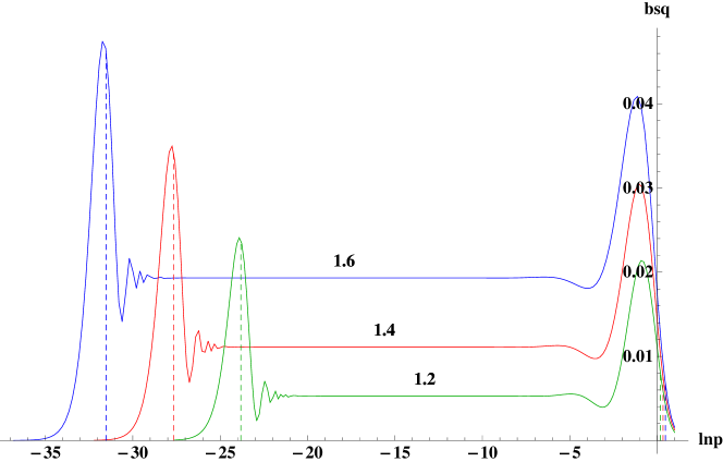
Figure 5.1: The exact solution $\left|\beta(p)\right|^{2}$ plotted against $\ln p$ for $m=1$, $t_{i}=0$, $t_{f}=20$ and $\omega={\color[rgb]{0,0,1}{1.6}},{\color[rgb]{1,0,0}{1.4}},{\color[rgb]{0,1,0}{1.2}}$.

The exact form of $\left|\beta(p)\right|^{2}$ is depicted in Figure 5.1 and Figure 5.2. The first figure shows $\left|\beta(p)\right|^{2}$ for three values of $\omega$, while the second uses three values of $t_{f}$. The rest of the parameters have the values $m=1$, $t_{i}=0$, $t_{f}=10$ and $\omega=1.5$.

These pictures show three regions of interest, corresponding to three different regimes:

1. $q\ll\omega$: $\left|\beta(p)\right|^{2}$ goes to $0$ as $pq$, as we shall prove in (5.2.10)

2. $p\gg\omega$: $\left|\beta(p)\right|^{2}$ goes to $0$ as $1/p^{4}$, (see (5.2.7))

3. $p\ll\omega\ll q$: $\left|\beta(p)\right|^{2}$ is remarcably well described by a constant value which we find to be a Fermi-Dirac distribution function, $(1+e^{2\pi m/\omega})^{-1}$ (5.2.13).

These regions are delimited by two resonances which occur roughly at $q\sim\omega$ and $p\sim\omega$.

Figure 5.2 shows three plots of different $t_{f}$, having the same parameters $m=1$, $t_{i}=0$ and $\omega=1.5$. The middle plateau and the second resonance overlap. This independence on the expansion time $\Delta t=t_{f}-t_{i}$ will be uncovered by the asymptotic analysis.

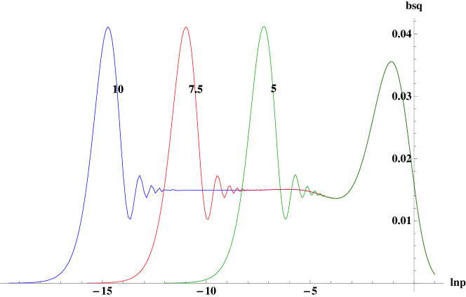
Figure 5.2: $\left|\beta(p)\right|^{2}$ plotted against $\ln p$ for $m=1$, $t_{i}=0$, $\omega=1.5$ and $t_{f}={\color[rgb]{0,0,1}{10}},{\color[rgb]{1,0,0}{7.5}},{\color[rgb]{0,1,0}{5.0}}$.

The large momentum region is investigated in Figure 5.4, where we show that $p^{4}\left|\beta(p)\right|^{2}$ approaches the value $m^{2}\omega^{2}/16$, indicated by black lines. This behaviour guarantees a finite number of particles per unit volume, since $n_{p}\sim p^{2}\left|\beta(p)\right|^{2}$. However, the volumic density of the energy $\mathcal{E}(\boldsymbol{x})$ (5.1.21a) has a logarithmic divergence. The spectral energy density $\mathcal{E}_{p}$ is plotted in Figure 5.4.

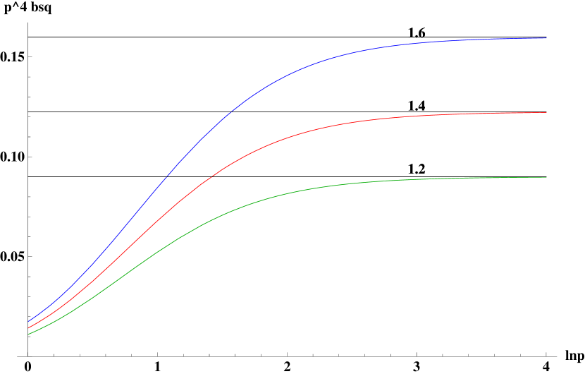
Figure 5.3: The particle number density $n_{p}=p^{2}\left|\beta(p)\right|^{2}$ is represented against $\ln p$ for $m=1$,$t_{i}=0$, $t_{f}=10$, $\omega={\color[rgb]{0,0,1}{1.6}},{\color[rgb]{1,0,0}{1.4}},{\color[rgb]{0,1,0}{1.2}}$.

Figure 5.4: the energy density $p^{2}E_{p}\left|\beta(p)\right|^{2}$ is plotted against $\ln p$ for $m=1$, $t_{i}=0$, $t_{f}=10$, $\omega={\color[rgb]{0,0,1}{1.6}},{\color[rgb]{1,0,0}{1.4}},{\color[rgb]{0,1,0}{1.2}}$.

5.2 Asymptotic analysis of the particle density

The analysis mainly involves the use of approximation formulas for the Hankel functions, given in Appendix A. Some of the more frequent notation used in this section are given below.

$$k=m/\omega,\qquad\nu_{\pm}=1/2\pm ik,\qquad\epsilon^{\pm}_{p}=(1\pm m/E_{p})^{1/2}$$

$$\Gamma_{\pm}(q,p)\text{ is defined in \eqref{eq:def_gammapm}},\quad\beta(p)\text{ is given in \eqref{eq:dirac_betaAB}},\quad H_{i}(q,p)\text{ are given by \eqref{eq:dirac_beta_H}}$$

We assume the reader has gone through section 4.2, and omit explanatory text that would otherwise be repeated.

5.2.1 Large momentum $p\gg\omega$

We find that $\left|\beta(p)\right|^{2}$ drops like $1/p^{4}$, which gives a logarithmic divergency of the energy of the created particles. This divergency might be explained by the sudden transition between the Minkowski and de Sitter phases. The analysis is done using the same method used in the scalar case: we substitute Hankel’s expansion (A.2.5) for the Hankel functions in the terms (5.1.24), for which we employ a similar notation:

$$H_{i}(q,p)=\frac{4\omega}{\pi\sqrt{pq}}\left(\cos\frac{q-p}{\omega}C_{i}(q,p)+\sin\frac{q-p}{\omega}S_{i}(q,p)\right)$$ (5.2.1)

with the functions $C_{i},P_{i}$ given by

$$C_{1} =\phantom{-}i\left(P^{+}_{q}Q^{+}_{p}-Q^{+}_{q}P^{+}_{p}\right) C_{2} =P^{+}_{q}P^{-}_{p}+Q^{+}_{q}Q^{+}_{p}$$ (5.2.2a)

$$S_{1} =-i\left(P^{+}_{q}P^{+}_{p}+Q^{+}_{q}Q^{+}_{p}\right) S_{2} =P^{+}_{q}Q^{-}_{p}-Q^{+}_{q}P^{-}_{p}$$ (5.2.2b)

The polynomials $Q,P$ are given by (A.2.5c),(A.2.5d). The notation $P^{\pm}_{p}$ stands for $P(\nu_{\pm},p/\omega)$. Contrary to the scalar case, the $C_{i},S_{i}$ functions are not real. We proceed in a similar fashion and express $\beta$ as a power series in $\omega$, keeping $\nu_{\pm}$ independent:

$$\beta(p)=\frac{i}{2}e^{-i(E_{q}t_{i}+E_{p}t_{f})}\sum_{n=0}^{\infty}\Omega^{(n)}(q,p)\omega^{n}$$ (5.2.3)

We shall retain terms up to $\omega^{2}$:

$$\Omega^{(0)}(q,p) =\cos\frac{q-p}{\omega}\mathcal{E}^{-++-}_{-}-i\sin\frac{q-p}{\omega}\mathcal{E}^{++--}_{-}$$

$$\Omega^{(1)}(q,p) =-\frac{ikm}{2}\left(\frac{1}{p}-\frac{1}{q}\right)\left(\cos\frac{q-p}{\omega}\mathcal{E}^{++--}_{-}-i\sin\frac{q-p}{\omega}\mathcal{E}^{-++-}_{-}\right)$$

$$-\frac{m}{2}\mathcal{E}^{++--}_{+}\left(\cos\frac{q-p}{\omega}\left(\frac{1}{p}-\frac{1}{q}\right)-i\sin\frac{q-p}{\omega}\left(\frac{1}{p}+\frac{1}{q}\right)\right)$$

$$\Omega^{(2)}(q,p) =-\frac{ik(k^{2}+1)}{4}\left\{\cos\frac{q-p}{\omega}\left(\frac{ik}{2}\left(\frac{1}{p}-\frac{1}{q}\right)^{2}\mathcal{E}^{++--}_{-}-\left(\frac{1}{p^{2}}-\frac{1}{q^{2}}\right)\mathcal{E}^{+--+}\right)\right.$$

$$\left.+i\sin\frac{q-p}{\omega}\left(\frac{1}{p^{2}}+\frac{1}{q^{2}}\right)\left(\frac{ik}{2}\mathcal{E}^{++--}_{-}+\mathcal{E}^{++--}_{+}\right)\right\}$$

$$+\frac{ik^{2}}{4qp}\sin\frac{q-p}{\omega}\left((1-k^{2})\mathcal{E}^{++--}_{-}+2ik\mathcal{E}^{++--}_{+}\right)$$

The terms $\mathcal{E}^{++--}_{-}$ stand for

$$\mathcal{E}^{rslm}_{\pm}=\epsilon^{r}_{q}\epsilon^{s}_{p}\pm\epsilon^{l}_{q}\epsilon^{m}_{p}\quad,\quad r,s,l,m\in\{-,+\}$$ (5.2.4)

We have used $4\nu_{\pm}^{2}-1=4ik(ik\pm 1)$, etc. The terms $\epsilon^{\pm}_{p}$ can be expressed in powers of $p$ as

$$\epsilon^{\pm}_{p}=1\pm\frac{m}{2E_{p}}+\frac{m^{2}}{8E_{p}^{2}}+\mathcal{O}(p^{-3}),$$

and so the $\Omega$ terms simplify to

$$\Omega^{(0)}(q,p) =m\mathcal{C}_{-}(q,p)+\mathcal{O}(p^{-3})$$ (5.2.5a)

$$\omega\Omega^{(1)}(q,p) =-\frac{ikm^{2}}{2}\left(\frac{1}{p}-\frac{1}{q}\right)\mathcal{C}_{+}(q,p)-m\mathcal{C}_{-}(q,p)+\mathcal{O}(p^{-3})$$ (5.2.5b)

$$\omega^{2}\Omega^{(2)}(q,p) =-\frac{im\omega(k^{2}+1)}{2}\left(\frac{1}{p}-\frac{1}{q}\right)\mathcal{C}_{+}(q,p)+\frac{m\omega}{qp}\sin\frac{q-p}{\omega}+\mathcal{O}(p^{-3})$$ (5.2.5c)

The recurrent terms are

$$\mathcal{C}_{\pm}(q,p)=\cos\frac{q-p}{\omega}\left(\frac{1}{p}\pm\frac{1}{q}\right)-i\sin\frac{q-p}{\omega}\left(\frac{1}{p}\mp\frac{1}{q}\right)$$ (5.2.5d)

We have used $k=m/\omega$. Summing the contributions, we are left with a leading term of order $1/p^{2}$, and thus we express $\beta$ as

$$\beta(p)=-\frac{m\omega}{4}e^{-i(E_{q}t_{i}+E_{p}t_{f})}\times\\ \left\{\cos\frac{q-p}{\omega}\left(\frac{1}{p^{2}}-\frac{1}{q^{2}}\right)-i\sin\frac{q-p}{\omega}\left(\frac{1}{p^{2}}+\frac{1}{q^{2}}\right)+\mathcal{O}(p^{-3})\right\}$$ (5.2.6)

All higher order terms contain $4\nu_{\pm}^{2}-1$, which is proportional to the mass of the field, and thus we confirm the result that there is no particle creation in the massless case (derived in subsection 4.1.3). For the case of sufficiently large expansion time $\Delta t=t_{f}-t_{i}$ we approximate the square of $\beta$ with $\left|\beta(p)\right|^{2}_{l}$ defined by

$$\left|\beta(p)\right|^{2}_{l}\xrightarrow[t_{f}\gg t_{i}]{}\frac{m^{2}\omega^{2}}{16p^{4}}$$ (5.2.7)

Although this dependency guarantees a finite total number of particles, this is not so with the total energy, which diverges.

5.2.2 Low momentum $q\ll\omega$

While a constant number of scalar particles are created in the low momentum region, the number of spinorial particles approaches $0$ as $p^{2}$.

In the limit $p\ll 0,q\ll 0$ we shall use the approximation (A.4.5) for the Hankel functions appearing in (5.1.24). The computation of $H_{2}$ is more demanding since the Hankel functions involved have different orders $\nu_{\pm}$. Nevertheless, it requires no special tricks, and the result is:

$$H_{1}(q,p) =\frac{4\sinh{\omega\Delta t\nu_{+}}}{i\pi\nu_{+}}$$ (5.2.8)

$$H_{2}(q,p) =\frac{2}{\pi\cosh{\pi k}}\sinh(\pi k-im\Delta t)\left(\sqrt{\frac{4\omega^{2}}{pq}}-\frac{1}{\left|\nu_{+}\right|^{2}}\sqrt{\frac{qp}{4\omega^{2}}}\right)+$$

$$\qquad\frac{2i}{\pi^{2}}\cosh{\frac{1}{2}\omega\Delta t}\left(\Gamma_{+}^{2}(q,p)/\nu_{-}-\Gamma_{-}^{2}(q,p)/\nu_{+}\right)$$ (5.2.9)

The square of $\beta$ is needlessly cumbersome to compute. We shall approximate the square roots appearing in (5.1.23) through $\epsilon^{\pm}_{p},\epsilon^{\pm}_{q}$ by their series expansion about $p/m=0$, ignoring terms of order $\mathcal{O}(p^{2})$:

$$\epsilon_{q}^{-}\epsilon_{p}^{-} \sim\frac{pq}{2m^{2}}\simeq 0 \epsilon_{q}^{+}\epsilon_{p}^{+} \simeq\sqrt{2}$$

$$\epsilon_{q}^{-}\epsilon_{p}^{+} \simeq\frac{q}{m} \epsilon_{q}^{+}\epsilon_{p}^{-} \simeq\frac{p}{m}$$

Substituting the above in the expression for $\beta$, we arrive at

$$\beta(p)\xrightarrow[q\ll 0]{}e^{-i(E_{q}t_{i}+E_{p}t_{f})}\frac{\sqrt{qp}}{m}\left\{\frac{\sinh{\omega\Delta t\nu_{+}}}{\nu_{+}}+\right.\\ \left.\frac{i}{2k\cosh{\pi k}}\left(e^{\omega\Delta t/2}\sinh(\pi k+im\Delta t)-e^{-\omega\Delta t/2}\sinh(\pi k-im\Delta t)\right)+\mathcal{O}(p^{2})\right\}$$ (5.2.10)

We have dropped a term of order $\mathcal{O}(p^{2})$. Therefore $\left|\beta(p)\right|^{2}$ goes to $0$ as $p^{2}$ for $q\ll\omega$.

5.2.3 Middle region $p\ll\omega\ll q$

The thermal spectrum of particle density not recovered in the scalar case emerges for the Dirac field in the middle region, subject to the constraint $p\ll m$. The flat plateau is given by a Fermi-Dirac distribution law of temperature $T=\omega/2\pi$, for the energy $E=m$.

Applying the same reasoning outlined in subsection 4.2.3, we use the first order approximation for large arguments of the Hankel functions entering in the coefficients $A,B$ of argument $q$, and thus arrive at

$$\tilde{A}(q,t_{i})\simeq-iE^{-iE_{q}t_{i}-iq/\omega+3i\pi/4}\quad,\quad\tilde{B}(q,t_{i})\simeq 0$$ (5.2.11)

Thus the $\beta$ coefficient reduces to

$$\beta(p)\xrightarrow[p\ll\omega\ll q]{}\tilde{B}(p,t_{f})$$ (5.2.12)

For a quick derivation of the thermal behaviour of $\left|\beta(p)\right|^{2}$, we may proceed by using only the term of order $p^{-1/2}$ in the expansion (A.4.5a), by which $\tilde{B}$ evaluates to

$$\tilde{B}(p,t_{f})\xrightarrow[p\ll\omega\ll q]{}\frac{i}{\sqrt{4\pi}}e^{-iE_{p}t_{f}}\left(\epsilon^{+}_{p}e^{-\pi k/2}\Gamma_{+}(p,p)-\epsilon^{-}_{p}e^{\pi k/2}\Gamma_{-}(p,p)\right)$$

and the square is

$$\left|\tilde{B}(p,t_{f})\right|^{2}\xrightarrow[p\ll\omega\ll q]{}\frac{1}{2}\left(1-\frac{m}{E_{p}}\tanh{\pi k}\right)-\frac{p}{4\pi E_{p}}\left(\Gamma_{+}^{2}(p,p)+\Gamma_{-}^{2}(p,p)\right)$$

The second term is at most $\pi^{2}/\cosh^{2}{\pi k}$, and is negligible for large enough mass or small enough expansion factor, but it becomes important as we depart from these conditions. However, this is not the “right” first order correction to $\left|\beta(p)\right|^{2}$, as we shall point out later in this section. The term $m/E_{p}$ can be expanded about $p/m=0$, and we arrive at

$$\left|\beta(p)\right|^{2}\xrightarrow[p\ll\omega\ll q]{}\frac{1}{e^{2\pi m/\omega}+1}+\mathcal{O}\left(p/m\right)$$ (5.2.13)

This resembles a Fermi-Dirac distribution function, if we let the energy equal $m$ (just as in our approximation), and interpret $\omega/2\pi$ as the temperature. This function approximates remarcably well the middle region where the condition $p\ll\omega\ll q$ is valid. However, the extreme regions of this plateau present two maxima that are highly pronounced when $\omega$ is small. In an attempt to approach this behaviour we consider both terms in the expansion (A.4.5a). Note that in this approximation the identity (A.4.4) is no longer valid. It is more convenient to first square $\tilde{B}(p,t_{f})$ and then apply the expansion of the Hankel functions:

$$\left|B(p,t_{f})\right|=\frac{\pi p}{8\omega}\left\{\mathcal{H}_{1}(p)-\frac{m}{E_{p}}\mathcal{H}_{2}(p)-\frac{p}{E_{p}}\mathcal{H}_{3}(p)\right\},$$

with the terms $\mathcal{H}_{i}$ given by

$$\mathcal{H}_{1}(p) =e^{\pi k}{H^{(2)}_{\nu_{+}}}{H^{(1)}_{\nu_{-}}}+e^{-\pi k}{H^{(2)}_{\nu_{-}}}{H^{(1)}_{\nu_{+}}}$$

$$\mathcal{H}_{2}(p) =e^{\pi k}{H^{(2)}_{\nu_{+}}}{H^{(1)}_{\nu_{-}}}-e^{-\pi k}{H^{(2)}_{\nu_{-}}}{H^{(1)}_{\nu_{+}}}$$

$$\mathcal{H}_{3}(p) =\phantom{e^{\pi k}}{H^{(2)}_{\nu_{+}}}{H^{(1)}_{\nu_{+}}}+\phantom{e^{-\pi k}}{H^{(2)}_{\nu_{-}}}{H^{(1)}_{\nu_{-}}}$$

Every Hankel function is understood to take the argument $p/\omega$. These functions evaluate to

$$\mathcal{H}_{1}(p) =\frac{4\omega}{\pi p}+\frac{p}{\omega\pi\left|\nu_{+}\right|^{2}}$$

$$\mathcal{H}_{2}(p) =-\frac{4\omega}{\pi p}\tanh{\pi k}+\frac{2}{i\pi^{2}}\left(\Gamma^{2}_{+}(p,p)/\nu_{-}-\Gamma^{2}_{-}/\nu_{+}\right)+\frac{p}{\pi\omega\left|\nu_{+}\right|^{2}}\tanh{\pi k}+\mathcal{O}(p^{2})$$

$$\mathcal{H}_{3}(p) =\frac{2\omega}{\pi^{2}p}\left(\Gamma^{2}_{+}(p,p)+\Gamma^{2}_{-}(p,p)\right)+\frac{4k}{\pi\left|\nu_{+}\right|^{2}}\tanh{\pi k}+\frac{p}{2\omega\pi^{2}}\left(\Gamma^{2}_{+}(p,p)/\nu_{-}^{2}+\Gamma^{2}_{-}(p,p)/\nu_{+}^{2}\right)$$

Since we are also interested in the behaviour of $\left|\beta(p)\right|^{2}$ near $p\sim\omega$, we cannot replace $E_{p}$ by $m$, and thus we settle to:

$$\left|\beta(p)\right|^{2}\xrightarrow[p\ll\omega\ll q]{}\left|\beta(p)\right|^{2}_{m}=\frac{1}{2}\left(1-\frac{m}{E_{p}}\tanh{\pi k}\right)-\frac{p}{8\pi E_{p}}\left(\Gamma^{2}_{+}(p,p)/\nu_{-}+\Gamma^{2}_{-}(p,p)/\nu_{+}\right)+\\ \frac{p^{2}}{8\omega^{2}\left|\nu_{+}\right|^{2}}\left(1-\frac{3m}{E_{p}}\tanh{\pi k}\right)-\frac{p^{3}}{16\pi\omega^{2}E_{p}}\left(\Gamma^{2}_{+}(p,p)/\nu^{2}_{-}+\Gamma^{2}_{-}(p,p)/\nu^{2}_{+}\right)+\dots$$ (5.2.14)

Note however that this expansion is not correct in the third order, but nevertheless it approaches the form of the exact solution better than if we would have omitted this contribution. There is no reference to the times $t_{i},t_{f}$, which means the form of $\left|\beta(p)\right|^{2}$ in the middle region is independent of the expansion time.

5.2.4 Resonances

There are three distinct regions of interest, for both the spinorial and the scalar case, separated by points situated roughly at $p\sim\omega$ and $q\sim\omega$. We have studied the asymptotic behaviour in these three regions in the preceding sections. This section is devoted to the analytical investigation of the pronounced maxima of produced fermions which occur at these points.

The analysis starts with the explicit form of $\left|\beta(p)\right|^{2}$, given in Equation 5.1.26. The extrema can be identified by setting $d\left|\beta(p)\right|^{2}/dp=0$. Since the functions $\mathcal{H}_{i}$ (defined by (5.1.27)) employed in the expression for $\left|\beta\right|^{2}$ have an explicit dependence on $q$ and $p$, we write the total derivative with respect to $p$ as

$$\frac{d}{dp}\mathcal{H}_{i}(q,p)=\left(\frac{\partial\mathcal{H}_{i}}{\partial p}\right)_{q}+\left(\frac{\partial\mathcal{H}_{i}}{\partial q}\right)_{p}$$

First we compute the derivatives of the coefficients of $\mathcal{H}_{i}$:

$$\frac{d}{dp}p =1 \frac{d}{dp}q =\frac{q}{p} \frac{d}{dp}qp =2q$$ (5.2.15a)

$$\frac{d}{dp}\frac{p}{E_{p}} =\frac{m^{2}}{E_{p}^{3}} \frac{d}{dp}\frac{q}{E_{q}} =\frac{qm^{2}}{pE_{q}^{3}} \frac{d}{dp}\frac{qp}{E_{q}E_{p}} =\frac{m^{2}q}{E_{q}E_{p}}\left(\frac{1}{E_{p}^{2}}+\frac{1}{E_{q}^{2}}\right)$$ (5.2.15b)

Next, we compute the derivatives of $H_{i}(q,p)$ (defined in (5.1.24)):

$$\frac{d}{dp}H_{1}(q,p) =\frac{i}{\omega p}\left(pH_{2}-qH_{2}^{*}\right)-\frac{2ik}{p}H_{1}-\frac{1}{p}H_{1}$$ (5.2.16a)

$$\frac{d}{dp}H_{2}(q,p) =\frac{i}{\omega p}\left(pH_{1}+qH_{1}^{*}\right)-\frac{1}{p}H_{2}$$ (5.2.16b)

With these we compute the derivatives of $\mathcal{H}_{i}$:

$$\frac{d}{dp}\mathcal{H}_{1}(q,p) =\frac{2i}{\omega}\left(H_{1}^{*}H_{2}-H_{1}H_{2}^{*}\right)-\frac{2iq}{\omega p}\left(H_{1}^{*}H_{2}^{*}-H_{1}H_{2}\right)-\frac{2}{p}\mathcal{H}_{1}$$ (5.2.17a)

$$\frac{d}{dp}\mathcal{H}_{2}(q,p) =\frac{i}{\omega}\left(H_{1}^{2}-H_{1}^{*\,2}+H_{2}^{2}-H_{2}^{*\,2}\right)+\frac{2ik}{p}\left(H_{1}^{*}H_{2}^{*}-H_{1}H_{2}\right)-\frac{2}{p}\mathcal{H}_{2}$$ (5.2.17b)

$$\frac{d}{dp}\mathcal{H}_{3}(q,p) =-\frac{iq}{\omega p}\left(H_{1}^{2}-H_{1}^{*\,2}-H_{2}^{2}+H_{2}^{*\,2}\right)+\frac{2ik}{p}\left(H_{1}^{*}H_{2}-H_{1}H_{2}^{*}\right)-\frac{2}{p}\mathcal{H}_{3}$$ (5.2.17c)

$$\frac{d}{dp}\mathcal{H}_{4}(q,p) =-\frac{2ik}{p}\left(H_{1}^{2}-H_{1}^{*\,2}\right)-\frac{2}{p}\mathcal{H}_{4}$$ (5.2.17d)

These derivatives satisfy the remarcable property

$$k^{2}\frac{d}{dp}\mathcal{H}_{1}(q,p)+k\frac{q}{\omega}\frac{d}{dp}\mathcal{H}_{2}(q,p)-k\frac{p}{\omega}\frac{d}{dp}\mathcal{H}_{3}(q,p)+\frac{qp}{\omega^{2}}\frac{d}{dp}\mathcal{H}_{4}(q,p)=\\ -\frac{2}{p}\left\{k^{2}\mathcal{H}_{1}(q,p)+k\frac{q}{\omega}\mathcal{H}_{2}(q,p)-k\frac{p}{\omega}\mathcal{H}_{3}(q,p)+\frac{qp}{\omega^{2}}\mathcal{H}_{4}(q,p)\right\}$$ (5.2.17e)

Using these results, the derivative of $\left|\beta\right|^{2}$ yields:

$$\frac{d}{dp}\left|\beta(p)\right|^{2}=\frac{\pi^{2}q}{32E_{q}E_{p}}\left\{-k^{2}\left(\frac{q^{2}}{E_{q}^{2}}+\frac{p^{2}}{E_{p}^{2}}\right)\mathcal{H}_{1}+\right.\\ \left.\left(1-\frac{q^{2}}{E_{q}^{2}}-\frac{p^{2}}{E_{p}^{2}}\right)\left(\frac{kq}{\omega}\mathcal{H}_{2}-\frac{kp}{\omega}\mathcal{H}_{3}\right)+qpk^{2}\left(\frac{1}{E_{q}^{2}}+\frac{1}{E_{p}^{2}}\right)\mathcal{H}_{4}\right\}$$ (5.2.18)

In the following subsections we shall work in the asymptotic cases $q\sim\omega\gg p$ and $p\sim\omega\ll q$, near the points where we hope to uncover the observed maxima.

First maximum $q\sim\omega\gg p$

We shall approximate the Hankel functions of argument $p/\omega$ with the first term in (A.4.5). In this approximation, all $\mathcal{H}_{i}$ functions are of order $1/p$, allowing us to eliminate terms with coefficients of order $p$ in (5.2.18):

$$\frac{d}{dp}\left|\beta(p)\right|^{2}\xrightarrow[p\rightarrow 0]{}\frac{\pi^{2}k^{2}q^{2}}{32E_{q}^{3}}\left(-\frac{q}{m}\mathcal{H}_{1}+\mathcal{H}_{2}\right)$$ (5.2.19)

The equation which determines the point of extremum is

$$\frac{q}{m}\mathcal{H}_{1}(q,p)=\mathcal{H}_{2}(q,p)$$ (5.2.20)

The functions $\mathcal{H}_{i}$ take the form

$$\mathcal{H}_{1}(q,p)\xrightarrow[p\rightarrow 0]{}-\frac{4\omega}{\pi p\cosh{\pi k}}\left\{\sinh{\pi k}\left(e^{\pi k}{H^{(2)}_{\nu_{+}}}{H^{(1)}_{\nu_{-}}}-e^{-\pi k}{H^{(2)}_{\nu_{-}}}{H^{(1)}_{\nu_{+}}}\right)-\right.\\ \left.\left({H^{(2)}_{\nu_{+}}}{H^{(2)}_{\nu_{-}}}+{H^{(1)}_{\nu_{+}}}{H^{(1)}_{\nu_{-}}}\right)\right\}$$ (5.2.21)

$$\mathcal{H}_{2}(q,p)\xrightarrow[p\rightarrow 0]{}-\frac{4\omega}{\pi p\cosh{\pi k}}\left\{\sinh{\pi k}\left({H^{(2)}_{\nu_{+}}}{H^{(1)}_{\nu_{+}}}+{H^{(2)}_{\nu_{-}}}{H^{(1)}_{\nu_{-}}}\right)+\phantom{\frac{1}{2}}\right.\\ \left.\frac{1}{2}e^{\pi k}\left({H^{(2)}_{\nu_{+}}}^{2}+{H^{(1)}_{\nu_{-}}}^{2}\right)-\frac{1}{2}e^{-\pi k}\left({H^{(2)}_{\nu_{-}}}^{2}+{H^{(1)}_{\nu_{+}}}^{2}\right)\right\}$$

The Hankel functions in the right-hand-side of the above expressions take the argument $q/\omega$. These forms are rather cumbersome to work with. Nevertheless, we find that the results obtained for large $\omega$ ($\nu_{\pm}\rightarrow 1/2$) give reasonably good predictions. In this limit, equation (5.2.20) takes the form

$$\sinh{\pi k}\left(1-\frac{q}{m}\sinh{\pi k}\right)=\left(\frac{q}{m}+\sinh{\pi k}\right)\cos{\frac{2q}{\omega}}$$

In the limit of large $\omega$, we can substitute $\sinh{\pi k}$ with $\pi k$, and thus we arrive at

$$p_{\text{max}}=\frac{\pi\omega}{4}e^{-\omega(t_{f}-t_{i})}$$ (5.2.22)

This formula becomes a good prediction only for $\omega>m$, but the predicted value falls farther away as we depart from this condition. Note that this value depends on the difference $t_{f}-t_{i}$.

Second maximum $p\sim\omega\ll q$

Although the position of the maximum situated at $q\sim\omega$ is given by a simple relation (5.2.22), we were unable to find a similar one for the maximum at $p\sim\omega$. However, we can extract several conclusions out of the asymptotic form of the equation which gives the point. In the region $p\sim\omega$, we can consider $q$ as infinitely large, and approximate the Hankel functions of argument $q/\omega$ with the asymptotic forms (A.2.3). In this approximation, all $\mathcal{H}_{i}$ functions are of order $1/q$, and thus we shall retain only the highest order in $q$ from (5.2.18):

$$\frac{d}{dp}\left|\beta(p)\right|^{2}\xrightarrow[q\rightarrow\infty]{}\frac{\pi^{2}k^{2}qp}{32E_{p}^{3}}\left(-\frac{p}{m}\mathcal{H}_{2}+\mathcal{H}_{4}\right)$$ (5.2.23)

The equation which determines the point of extremum is

$$\frac{p}{m}\mathcal{H}_{2}(q,p)=\mathcal{H}_{4}(q,p)$$ (5.2.24)

This is very similar to equation (5.2.20), which determines the point of maximum at $q\sim\omega$. We proceed in a similar fashion, and evaluate the functions $\mathcal{H}_{i}$:

$$\mathcal{H}_{2}(q,p) \xrightarrow[q\rightarrow\infty]{}-\frac{4\omega}{\pi q}\left(e^{\pi k}{H^{(2)}_{\nu_{+}}}{H^{(1)}_{\nu_{-}}}-e^{-\pi k}{H^{(2)}_{\nu_{-}}}{H^{(1)}_{\nu_{+}}}\right)$$ (5.2.25a)

$$\mathcal{H}_{4}(q,p) \xrightarrow[q\rightarrow\infty]{}-\frac{4\omega}{\pi q}\left({H^{(2)}_{\nu_{+}}}{H^{(1)}_{\nu_{+}}}+{H^{(2)}_{\nu_{-}}}{H^{(1)}_{\nu_{-}}}\right)$$ (5.2.25b)

It is understood that the Hankel functions take the argument $p/\omega$. This gives accurate results as long as we have corresponding numerical software to solve the equation (5.2.24).

Taking the limit $\omega\rightarrow\infty$ (with $m$ finite) simplifies (5.2.25) to

$$\mathcal{H}_{2}(q,p)\xrightarrow[\begin{subarray}{c}q\rightarrow\infty\\ m\ll\omega\end{subarray}]{}-\frac{16\omega^{2}}{\pi^{q}p}\sinh{\pi k}\quad,\quad\mathcal{H}_{4}(q,p)\xrightarrow[\begin{subarray}{c}q\rightarrow\infty\\ m\ll\omega\end{subarray}]{}-\frac{16\omega^{2}}{\pi^{q}p}$$ (5.2.26)

This predicts the maximum at

$$p_{\text{max}}=\frac{\omega}{\pi}$$ (5.2.27)

This result is not accurate, since for increasing $\omega$ it predicts a shift to the right for the point of maximum, which contravenes numerical results by which we find that the point actually shifts to the left. However, there is one important conclusion to be drawn: the position of the maximum does not depend on $t_{i}$ nor on $t_{f}$, as long as $t_{f}-t_{i}$ is sufficiently large to regard $q/\omega$ as approaching infinity.

A further approximation can be done by assuming that $p/\omega<1$ (which is not true for small masses). In this case we substitute (A.4.5) in (5.2.25) and arrive at

$$\mathcal{H}_{2} \xrightarrow[\begin{subarray}{c}q\rightarrow\infty\\ p\ll\omega\end{subarray}]{}-\frac{4\omega}{\pi^{2}q}\left\{\left(\frac{4\omega}{p}-\frac{p}{\omega\left|\nu_{+}\right|^{2}}\right)\tanh{\pi k}+\frac{2i}{\pi}\left(\frac{\Gamma_{+}^{2}(p,p)}{\nu_{-}}-\frac{\Gamma_{-}^{2}(p,p)}{\nu_{+}}\right)\right\}$$

$$\mathcal{H}_{4} \xrightarrow[\begin{subarray}{c}q\rightarrow\infty\\ p\ll\omega\end{subarray}]{}-\frac{4\omega}{\pi^{3}q}\left\{\frac{2\omega}{p}\left(\Gamma_{+}^{2}(p,p)+\Gamma_{-}^{2}(p,p)\right)+\frac{p}{2\omega}\left(\frac{\Gamma_{+}^{2}(p,p)}{\nu_{-}^{2}}+\frac{\Gamma_{-}^{2}(p,p)}{\nu_{+}^{2}}\right)+\frac{4\pi k}{\left|\nu_{+}\right|^{2}}\tanh{\pi k}\right\}$$

Substituting in (5.2.23), the derivative of $\left|\beta\right|^{2}$ follows:

$$\frac{d}{dp}\left|\beta(p)\right|^{2}\xrightarrow[\begin{subarray}{c}q\rightarrow\infty\\ p\ll\omega\end{subarray}]{}\frac{m^{2}}{8E_{p}^{3}}\left\{-\frac{2}{\pi}\left(\Gamma_{+}^{2}(p,p)+\Gamma_{-}^{2}(p,p)\right)+\frac{\tanh{\pi k}}{k\left|\nu_{+}\right|^{2}}\frac{p}{\omega}+\right.\\ \left.\left(\frac{i}{k\pi}\left(\frac{\Gamma_{+}^{2}(p,p)}{\nu_{-}^{2}}-\frac{\Gamma_{-}^{2}(p,p)}{\nu_{+}^{2}}\right)+\frac{3}{2\pi}\left(\frac{\Gamma_{+}^{2}(p,p)}{\nu_{-}^{2}}+\frac{\Gamma_{-}^{2}(p,p)}{\nu_{+}^{2}}\right)\right)\frac{p^{2}}{\omega^{2}}-\frac{\tanh{\pi k}}{k\left|\nu_{+}\right|^{2}}\frac{p^{3}}{\omega^{3}}\right\}$$ (5.2.28)

Analytically, nothing much is gained because of the presence of the functions $\Gamma_{\pm}(p,p)$ (defined by (A.4.6)). However, if the ratio $\omega/m$ is not less than $1/2$, we obtain good predictions for the position of the maximum. If $m$ is increased, the point of maximum becomes larger than $\omega$, and the approximation $p\ll\omega$ is no longer valid. This region is not accessible by this method.

5.2.5 The number of created particles

Because the asymptotic form for the middle region $p\ll\omega\ll q$ contains $E_{p}$, which cannot be replaced by a series expansion in powers of $p$. Such an expansion departs too much from the exact solution. A second difficulty is related to the choice of the value $p_{\nu}$ at which the transition between the middle and the large asymptotic forms is to be made. Because the “order 0” term in (5.2.14) contains the energy $E_{p}$, it is difficult to solve the equation $\left|\beta(p)\right|^{2}_{l}(p_{\nu})=\left|\beta(p)\right|^{2}_{m}(p_{\nu})$ even in the first order. We propose, as in the scalar case, to have $p_{\nu}$ determined numerically, such that the equation is satisfied. The transition between $\left|\beta(p)\right|^{2}_{s}$ and $\left|\beta(p)\right|^{2}_{m}$ will be done at $q=\omega e^{-\omega/2}$, because the asymptotic form for small $p$ exhibits a violent increase, following the increase in $\left|\beta(p)\right|^{2}$ (corresponding to the appearence of the first resonance at $q=\pi\omega/4$, given by (5.2.22)).

$$\left|\beta(p)\right|^{2}_{as}=\begin{cases}\left|\beta(p)\right|^{2}_{s}&q<\omega e^{-\omega/2}\\ \left|\beta(p)\right|^{2}_{m}&\omega e^{-\omega/2}<q\text{and}p<p_{\nu}\\ \left|\beta(p)\right|^{2}_{l}&p>p_{\nu}\end{cases},$$ (5.2.29)

$$\left|\beta(p)\right|^{2}_{l}(p_{\nu})=\left|\beta(p)\right|^{2}_{m}(p_{\nu}).$$ (5.2.30)

Performing the integral of $\left|\beta(p)\right|^{2}_{m}$ brings little insight because of the terms containing products of $\Gamma_{\pm}(p,p)/E_{p}$, which give integrals of the form

$$\int\frac{x^{a}}{\sqrt{x^{2}+1}}dx=\frac{x^{a+1}}{a+1}{}_{2}F_{1}\left(\frac{1+a}{2},\frac{1}{2};1+\frac{1+a}{2};-x^{2}\right).$$ (5.2.31)

For numerical values of the number of particles we rely on numerical computation results, which we shall present in the following subsection.

5.2.6 Graphical comparison to the exact solution

In the following we shall present graphical illustrations of the results of the previous subsections. We begin by representing the middle region (Figure 5.5) through a plot of $\left|\beta(p)\right|^{2}$ for large $\omega$. The plateau is described by a Fermi-Dirac distribution function $(e^{2\pi k}+1)^{-1}$ (5.2.13), represented in dark colour.

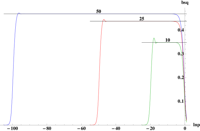
Figure 5.5: $\left|\beta(p)\right|^{2}$ represented against $\ln p$ for $\omega={\color[rgb]{0,0,1}{50}},{\color[rgb]{1,0,0}{25}},{\color[rgb]{0,1,0}{10}}$. The dark horizontal lines represent the Fermi-Dirac distribution function of temperature $\omega/2\pi$ and energy $m$.

The low-energy resonance, given by $q=\pi\omega/4$ (5.2.22) are indicated through blue dots in Figure 5.6. The formula used is not accurate for $\omega<1.5$, in which case the points have a tendency to shift left. But for high $\omega$, the approximation becomes reliable.

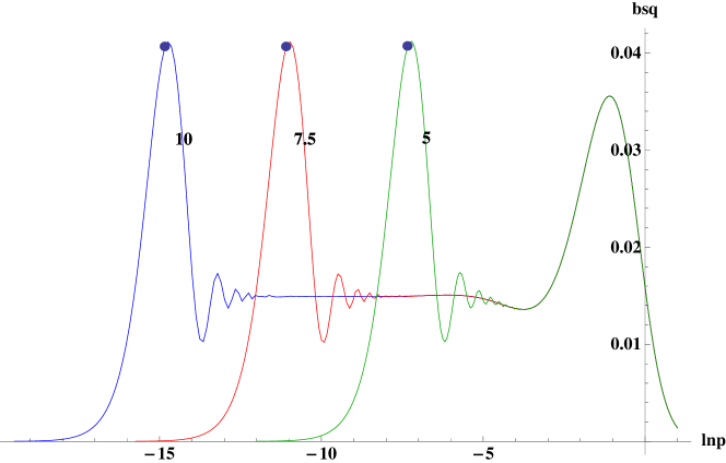
Figure 5.6: $\left|\beta(p)\right|^{2}$ plotted against $\ln p$ for $m=1$, $t_{i}=0$, $\omega=1.5$ and $t_{f}={\color[rgb]{0,0,1}{10}},{\color[rgb]{1,0,0}{7.5}},{\color[rgb]{0,1,0}{5.0}}$. Blue dots indicate the predicted points of maxima.

The asymptotic form $\eqref{eq:dirac_bsqas}$ is compared with the exact solution in Figure 5.7. The first maximum is not well captured, and there are (important) differences near $p\sim\omega$.

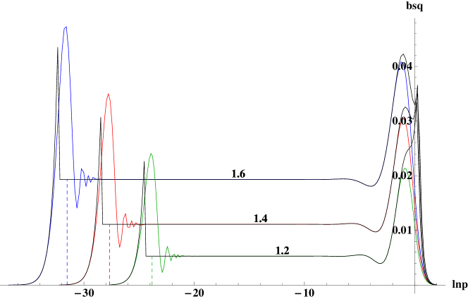
Figure 5.7: lin-log plot $\omega={\color[rgb]{0,0,1}{50}},{\color[rgb]{1,0,0}{25}},{\color[rgb]{0,1,0}{10}}$

The value $p_{\nu}$ at which the transition between the middle and the large asymptotic forms occurs has been numerically computed using (5.2.30). We give the dependency of $p_{\nu}$ on $m$ (Figure 5.9) and on $\omega$ (Figure 5.9).

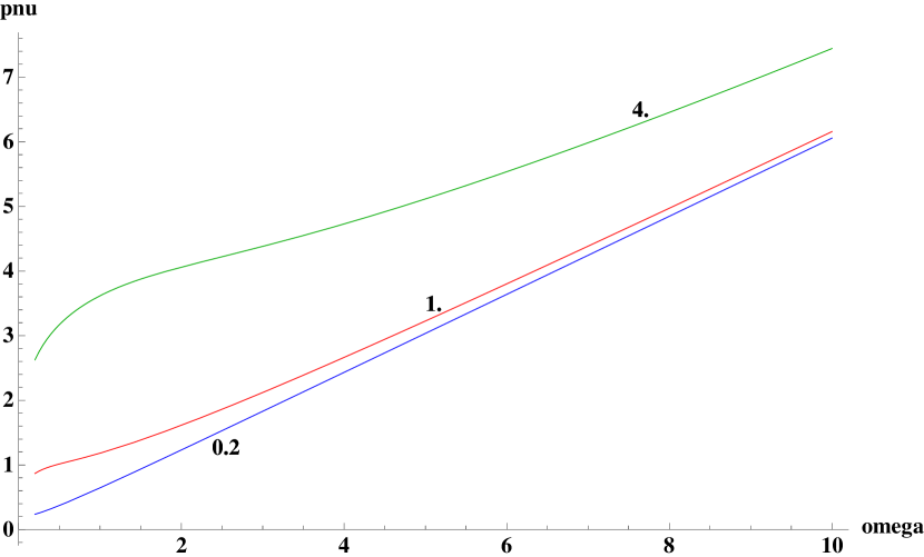
Figure 5.8: $p_{\nu}$ plotted against $\omega$ for $m={\color[rgb]{0,0,1}{0.2}},{\color[rgb]{1,0,0}{1}},{\color[rgb]{0,1,0}{4}}$.

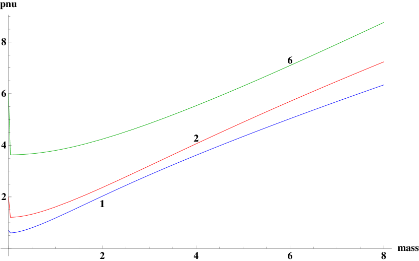
Figure 5.9: $p_{\nu}$ plotted against $m$ for $\omega={\color[rgb]{0,0,1}{1}},{\color[rgb]{1,0,0}{2}},{\color[rgb]{0,1,0}{6}}$.

We show in more detail the amount of displacement between the asymptotic form and the exact solution near $p\sim\omega$ for $\left|\beta(p)\right|^{2}$ (Figure 5.11) and for the particle number density $2/\pi^{2}p^{2}\left|\beta(p)\right|^{2}$ (Figure 5.11).

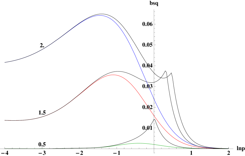
Figure 5.10: The dark lines represent $\left|\beta(p)\right|^{2}_{as}$, which we compare to $\left|\beta(p)\right|^{2}$ for $\omega={\color[rgb]{0,0,1}{2}},{\color[rgb]{1,0,0}{1.5}},{\color[rgb]{0,1,0}{0.5}}$.

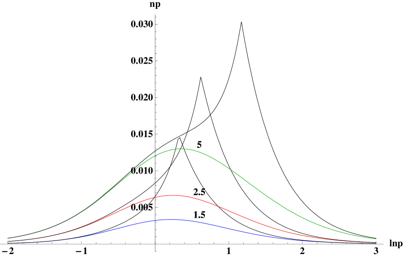
Figure 5.11: The asymptotic form of $n_{p}$ (plotted in black) is compared to the exact $n_{p}$ at $\omega={\color[rgb]{0,0,1}{1.5}},{\color[rgb]{1,0,0}{2.5}},{\color[rgb]{0,1,0}{5}}$.

Next we turn our attention to the particle number volumic density:

$$n(\boldsymbol{x})=\int_{0}^{\infty}\frac{2}{\pi^{2}}p^{2}\,\left|\beta(p)\right|^{2}.$$

The displacement between the asymptotic form and the exact solution causes an increase in the asymptotic particle number density by a factor. This factor can be read off from the logarithmic plot in Figure 5.12, where we show the result of the numerical integration $\ln n(\boldsymbol{x})$ as a function of $m$, at $t_{i}=0$, $t_{f}=10$ and $\omega=1.0$. We find that by dividing the asymptotic value through $1.8$ the two curves overlap on most of the domain.

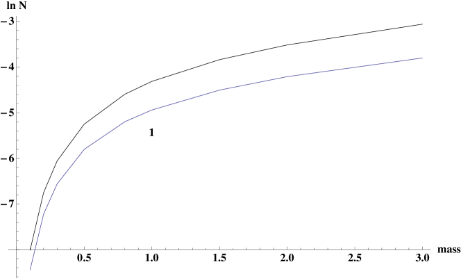
Figure 5.12: $\ln n(\boldsymbol{x})$ as a function of the particle mass $m$ at $\omega=1$. The blue curve represents the exact solution, while the asymptotic one is reprezented using dark colour.

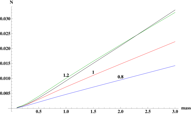
Figure 5.13: $n(\boldsymbol{x})$ as a function of the particle mass $m$ for $\omega={\color[rgb]{0,0,1}{0.8}},{\color[rgb]{1,0,0}{1.0}},{\color[rgb]{0,1,0}{1.2}}$ (the asymptotic solution, plotted in dark colour, is divided by $2.0$)

In Figure 5.13 we show the particle number density $n(\boldsymbol{x})$ as a function of the particle mass for different $\omega$, and in Figure 4.12 we plot against $\omega$ for different $m$. The other parameters are $t_{i}=0$ and $t_{f}=10$.

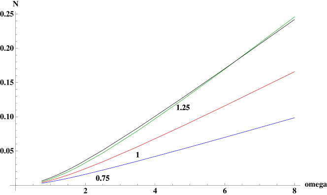
Figure 5.14: $n(\boldsymbol{x})$ as a function of the expansion factor $\omega$ for $m={\color[rgb]{0,0,1}{0.75}},{\color[rgb]{1,0,0}{1.00}},{\color[rgb]{0,1,0}{1.25}}$ (asymptotic solution is divided by $1.5$)

We conclude that there is no dependency on the expansion time $t_{f}$, as long as $\omega\Delta t>1$. There is a monotonic increase of $n(\boldsymbol{x})$ for increasing $m$ and $\omega$, and we expect it to approach $0$ as $m\rightarrow 0$ or $\omega\rightarrow 0$. Unfortunately, numerical limitations prevent us from exploring the behaviour of $\left|\beta(p)\right|^{2}$ for small $\omega$ or for large $m$, and the numerical integration fails to converge when using large $\omega$. Because of the logarithmic divergence of $p^{3}\left|\beta(p)\right|^{2}$, the volumic density of energy is infinite. A possible explanation for this is that the sudden change in the metric, happening in an infinitely short time, produces an infinite amount of energy.

Chapter 6 Conclusion

In this chapter we summarize our results and point out possibilities for further development.

We have investigated the phenomenon of particle production by a time-dependent gravitational field of finite extension. In the following we shall present our results sepparatelly for the scalar and the spinorial field.

A common result, which we have confirmed in subsection 4.1.3 and subsection 5.1.3, is that there is no particle production for conformal fields (i.e. conformally coupled massless scalar field, and massless spinorial field).

In both cases we identify three different regimes. We shall refer to the region $q\ll\omega$ as the low momentum (or far infrared) region, to $p\ll\omega\ll q$ as the middle region and to the region $\omega\ll p$ as the large momentum (ultraviolet) region.

The quantity $\left|\beta(p)\right|^{2}$ and all subsequent quantities derived from it ($n(\boldsymbol{x})$, $\mathcal{E}(\boldsymbol{x})$) depend only on the time extension of the expansion phase $\Delta t=t_{f}-t_{i}$. For $\Delta t$ of the order of the Hubble time $1/\omega$, quantities of the form $p^{a}\left|\beta(p)\right|^{2}$ (a = 2,3) approach a constant form, and quantities resulting from integration ($n(\boldsymbol{x})$, $\mathcal{E}(\boldsymbol{x})$) become independent of $\Delta t$.

For the scalar field, we have identified two regimes, corresponding to the positiveness of $\mu=1/4-m^{2}/\omega^{2}-12(\xi-1/6)$. We shall refer to the regime corresponding to $\mu>0$ as hyperbolic, and to $\mu<0$ as trigonometric.

In the low-momentum limit $\left|\beta(p)\right|^{2}$ approaches a constant value, which increases exponentially with the time extension $\Delta t$ and the expansion factor $\omega$ in the hyperbolic regime, following the hyperbolic sine law (4.2.21). If $\mu<0$, the argument of the hyperbolic sine is imaginary, and we uncover an oscillatory behaviour.

There is a transition occuring in the middle region. There is a rapid descent from the high value attained in the hyperbolic case, following a power law $(2\omega/p)^{2\nu}$ (4.2.26). In the trigonometric regime, $\left|\beta(p)\right|^{2}$ oscillates around a constant term with a roughly constant amplitude. The constant term resembles a Bose-Einstein distribution function, but we find a polynomial correction of order $\omega^{2}/m^{2}$, which eliminates the strong suppresion characteristic to thermal distributions (4.2.31), and the exact form does not diverge near $\nu=0$, where the approximation is not valid.

In the large-momentum limit we find that $\left|\beta(p)\right|^{2}$ goes to $0$ as $1/p^{n}$, with $n=6$ for the conformal case and $n=4$ for any other case. This assures a finite particle density $n(\boldsymbol{x})$, but the energy exhibits a logarithmic divergence when using non-conformal coupling. In the following we shall refer only to the conformally coupled case.

The particle number density $n(\boldsymbol{x})$ grows linearly with the particle mass $m$ (4.2.39) and quadratically with the expansion parameter $\omega$ (4.2.37). We have derived an asymptotic form for $n(\boldsymbol{x})$, but cannot confirm its validity in the high $\omega$ or high $m$ limits because of insuficient accuracy of the numerical methods used in evaluating the exact solution. The energy has a stronger increase with $m$.

In the low momentum limit of the spinorial case, $\left|\beta(p)\right|^{2}$ goes to $0$ as $p^{2}$ (5.2.10).

The middle region is a plateau which follows a Fermi-Dirac distribution law in the approximation $p\ll\omega$ and $m/\omega\ll 1$. The temperature is equal to $\omega/2\pi$ and the particle energy is $m$ (5.2.13).

For large momentum, $\left|\beta(p)\right|^{2}$ goes to $0$ as $1/p^{4}$, which ensures a finite particle number density $n(\boldsymbol{x})$, but gives a logarithmic divergence for the energy $\mathcal{E}(\boldsymbol{x})$.

The particle number density increases roughly linear with the mass of the particles (see Figure 5.13) and with the expansion factor (see Figure 5.14). Asymptotic analysis revealed a quadratic increase of the number density for large enough values of the expansion factors, but this prediction could not be verified because of numerical instability.

The logarithmic divergence of the energy for the non-conformally coupled scalar and spinorial fields may be attributed to the unphysical instantaneous transition between the Minkowski flat regions and the de Sitter expansion phase.

Further analysis can be made on the Dirac field asymptotic forms, especially to the integrals for the particle number density and the energy density. Some discussion is needed to clarify the nature of the divergence of the energy. The constant value it approaches in the conformally coupled scalar case suggests a comparison between our result and the Friedmann equations of the de Sitter space. Our work has laid the basis for the investigation of particle production in external gauge fields (e.g. a Coulomb field).

Appendix A Properties of Hankel functions

This appendix is intended to provide a reference for the properties of the Hankel functions required for the development of this paper.

A.1 Differential equation

In this section we present the construction of the Hankel functions as well as some important relations between them. The Hankel functions are solutions to the Bessel equation [bookpart:smirnov_bess]:

$$\left(z^{2}\frac{d^{2}}{dz^{2}}+z\frac{d}{dz}+(z^{2}-\nu^{2})\right)Z_{p}(z)=0.$$ (A.1.1)

The series solutions to the above equation are the Bessel functions of order $\pm\nu$:

$$J_{\pm\nu}(z)=\left(\frac{z}{2}\right)^{\pm\nu}\sum_{k=0}^{\infty}\frac{(-1)^{k}}{k!\Gamma{k\pm\nu+1}}\left(\frac{z}{2}\right)^{2k}.$$ (A.1.2)

The complex conjugate passes onto the order and the argument:

$$J_{\nu}(z)^{*}=J_{\nu^{*}}(z^{*}).$$ (A.1.3)

The wronskian [bookpart:watson_wronsk] of the Bessel functions of opposite order is:

$$W(J_{-\nu},J_{\nu})=\frac{\mathcal{C}}{z}=\frac{2\sin{\nu\pi}}{\pi z}.$$ (A.1.4)

The two solutions of order $\nu$ and $-\nu$ are linearly independent when $\nu$ is not an integer (because the wronskian is non-zero). When $\nu=n$ is an integer, the two functions are linearly dependent, since they are related by

$$J_{-n}(z)=(-1)^{n}J_{n}(z).$$ (A.1.5)

Bessel functions of the second kind, or Neumann functions, can be constructed using $J_{\pm\nu}$:

$$N_{\nu}(z)=\frac{J_{\nu}(z)\cos{\nu\pi}-J_{-\nu}(z)}{\sin{\nu\pi}}.$$ (A.1.6)

Using (A.1.3), we see that the complex conjugate passes onto the order and the argument:

$$N_{\nu}(z)^{*}=N_{\nu^{*}}(z^{*}).$$ (A.1.7)

The wronskian of Neumann functions of opposite order follows:

$$W(N_{-\nu},N_{\nu})=\frac{-2\cos^{2}{\pi\nu}+2}{\pi z\sin{\pi\nu}}=\frac{2\sin{\nu\pi}}{\pi z}.$$ (A.1.8)

The wronskian with the bessel function of the same order is

$$W(J_{\nu},N_{\nu})=W(J_{-\nu},J_{\nu})/\sin{\nu\pi}=\frac{2}{\pi z}.$$ (A.1.9)

Therefore, the two functions are always linearly independent.

The wronskian with the bessel function of opposite order is

$$W(J_{-\nu},N_{\nu})=W(J_{-\nu},J_{\nu})\cos{\nu\pi}/\sin{\nu\pi}=\frac{2\cos{\nu\pi}}{\pi z}.$$ (A.1.10)

Bessel functions of the third kind [book:jackson], or Hankel functions are constructed with these two linear independent solutions:

$${H^{(1)}_{\nu}}(z) =J_{\nu}(z)+iN_{\nu}(z)$$ Hankel function of the first kind (A.1.11a)

$${H^{(2)}_{\nu}}(z) =J_{\nu}(z)-iN_{\nu}(z)$$ Hankel function of the second kind (A.1.11b)

The wronskian of the two kinds of Hankel functions is

$$W({H^{(1)}_{\nu}},{H^{(2)}_{\nu}})=-2iW(J_{\nu},N_{\nu})=-\frac{4i}{\pi z}.$$ (A.1.12)

Complex conjugation passes to the order and argument and switches between the two kinds of Hankel functions:

$${H^{(1)}_{\nu}}(z)^{*}={H^{(2)}_{\nu^{*}}}(z^{*}),\qquad{H^{(2)}_{\nu}}(z)^{*}={H^{(1)}_{\nu^{*}}}(z^{*}).$$ (A.1.13)

Replacing the Neumann function (A.1.6) in (A.1.11) we obtain an alternative form for the Hankel functions:

$${H^{(1)}_{\nu}}(z)=\frac{i}{\sin{\nu\pi}}\left(J_{\nu}(z)e^{-i\nu\pi}-J_{-\nu}(z)\right),\qquad{H^{(2)}_{\nu}}(z)=\frac{-i}{\sin{\nu\pi}}\left(J_{\nu}(z)e^{i\nu\pi}-J_{-\nu}(z)\right).$$

From this form we can read the connection between ${H^{(1,2)}_{-\nu}}$ and ${H^{(1,2)}_{\nu}}$:

$${H^{(1)}_{-\nu}}(z)=e^{i\nu\pi}{H^{(1)}_{\nu}}(z),\qquad{H^{(2)}_{-\nu}}(z)=e^{-i\nu\pi}{H^{(2)}_{\nu}}(z).$$ (A.1.14)

Denoting by $\Omega_{\nu}$ any of the Bessel functions introduced so far, the following relations stand:

$$\Omega_{\nu-1}(z)+\Omega_{\nu+1}(z)=\frac{2\nu}{z}\Omega_{\nu}(z),$$ (A.1.15a)

$$\Omega_{\nu-1}(z)-\Omega_{\nu+1}(z)=2\Omega^{\prime}_{\nu}(z),$$ (A.1.15b)

$$\Omega^{\prime}_{\nu}(z)=\Omega_{\nu-1}(z)-\frac{\nu}{z}\Omega_{\nu}(z),$$ (A.1.15c)

$$\Omega^{\prime}_{\nu}(z)=-\Omega_{\nu+1}(z)+\frac{\nu}{z}\Omega_{\nu}(z).$$ (A.1.15d)

A common example of Hankel functions is that of order $\nu=1/2$:

$${H^{(1)}_{1/2}} =-i\sqrt{\frac{2}{\pi z}}e^{iz},$$ (A.1.16a)

$${H^{(2)}_{1/2}} =\phantom{-}i\sqrt{\frac{2}{\pi z}}e^{-iz}.$$ (A.1.16b)

A.2 Asymptotic forms

In this section we give the asymptotic forms for small and large values of the argument, corresponding to the Hankel functions and their derivatives.

For small values of the argument we have [bookpart:zwillinger_bessel]:

$${H^{(1)}_{\nu}}(z) =\phantom{-}\left(\frac{2}{z}\right)^{\nu}\frac{\Gamma(\nu)}{i\pi}+\left(\frac{z}{2}\right)^{\nu}\frac{1+i\cot(\pi\nu)}{\Gamma(1+\nu)}+\mathcal{O}(z^{2\pm\nu}),$$ (A.2.1a)

$${H^{(2)}_{\nu}}(z) =-\left(\frac{2}{z}\right)^{\nu}\frac{\Gamma(\nu)}{i\pi}+\left(\frac{z}{2}\right)^{\nu}\frac{1-i\cot(\pi\nu)}{\Gamma(1+\nu)}+\mathcal{O}(z^{2\pm\nu}).$$ (A.2.1b)

The derivatives of the Hankel functions can be approximated by:

$${H^{(1)}_{\nu}}(z)^{\prime} =-\frac{\nu}{z}\left(\phantom{-}\left(\frac{2}{z}\right)^{\nu}\frac{\Gamma(\nu)}{i\pi}-\left(\frac{z}{2}\right)^{\nu}\frac{1+i\cot(\pi\nu)}{\Gamma(1+\nu)}\right)+\mathcal{O}(z^{2\pm\nu}),$$ (A.2.2a)

$${H^{(2)}_{\nu}}(z)^{\prime} =-\frac{\nu}{z}\left(-\left(\frac{2}{z}\right)^{\nu}\frac{\Gamma(\nu)}{i\pi}-\left(\frac{z}{2}\right)^{\nu}\frac{1-i\cot(\pi\nu)}{\Gamma(1+\nu)}\right)+\mathcal{O}(z^{2\pm\nu}).$$ (A.2.2b)

For large values of the argument we can use [book:abramowitzstegun]:

$${H^{(1)}_{\nu}}(z) =\sqrt{\frac{2}{\pi z}}e^{i(z-\nu\pi/2-\pi/4)}\left(1+\mathcal{O}(z^{-1})\right),$$ (A.2.3a)

$${H^{(2)}_{\nu}}(z) =\sqrt{\frac{2}{\pi z}}e^{-i(z-\nu\pi/2-\pi/4)}\left(1+\mathcal{O}(z^{-1})\right).$$ (A.2.3b)

The derivatives of the Hankel functions are simply

$${H^{(1)}_{\nu}}(z)^{\prime} =i\sqrt{\frac{2}{\pi z}}e^{i(z-\nu\pi/2-\pi/4)}\left(1+\mathcal{O}(z^{-1})\right),$$ (A.2.4a)

$${H^{(2)}_{\nu}}(z)^{\prime} =-i\sqrt{\frac{2}{\pi z}}e^{i(z-\nu\pi/2-\pi/4)}\left(1+\mathcal{O}(z^{-1})\right).$$ (A.2.4b)

Hankel’s expansion is given by:

$${H^{(1)}_{\nu}}(z) =\sqrt{\frac{2}{\pi z}}(P(\nu,z)+iQ(\nu,z))e^{i\chi},$$ (A.2.5a)

$${H^{(2)}_{\nu}}(z) =\sqrt{\frac{2}{\pi z}}(P(\nu,z)-iQ(\nu,z))e^{-i\chi},$$ (A.2.5b)

with

$$P(\nu,z) \xrightarrow[z\rightarrow\infty]{}\sum_{k=0}^{\infty}(-1)^{k}\frac{(\nu,2k)}{(2z)^{2k}}$$

$$=1-\frac{(\mu-1)(\mu-9)}{2!(8z)^{2}}+\frac{(\mu-1)(\mu-9)(\mu-25)(\mu-49)}{4!(8z)^{4}}+\mathcal{O}(z^{-6}),$$ (A.2.5c)

$$Q(\nu,z) \xrightarrow[z\rightarrow\infty]{}\sum_{k=0}^{\infty}(-1)^{k}\frac{(\nu,2k+1)}{(2z)^{2k+1}}$$

$$=\frac{\mu-1}{8z}-\frac{(\mu-1)(\mu-9)(\mu-25)}{3!(8z)^{3}}++\mathcal{O}(z^{-5}),$$ (A.2.5d)

$$(\alpha,n) =-\frac{(n-1/2)^{2}-\alpha^{2}}{n}(\alpha,n-1),\qquad(\alpha,0)=1,$$

$$\chi =z-\frac{\pi\nu}{2}-\frac{\pi}{4},$$

$$\mu =4\nu^{2}.$$

Hankel’s expansion for the derivatives is:

$${H^{(1)}_{\nu}}^{\prime}(z) =i\sqrt{\frac{2}{\pi z}}(R(\nu,z)+iS(\nu,z))e^{i\chi},$$ (A.2.6a)

$${H^{(2)}_{\nu}}^{\prime}(z) =-i\sqrt{\frac{2}{\pi z}}(R(\nu,z)-iS(\nu,z))e^{-i\chi},$$ (A.2.6b)

with

$$R(\nu,z) \xrightarrow[z\rightarrow\infty]{}\sum_{k=0}^{\infty}(-1)^{k}\frac{4\nu^{2}+16k^{2}-1}{4\nu^{2}-(4k-1)^{2}}\frac{(\nu,2k)}{(2z)^{2k}}$$

$$=1-\frac{(\mu-1)(\mu+15)}{2!(8z)^{2}}+\mathcal{O}(z^{-4}),$$ (A.2.6c)

$$S(\nu,z) \xrightarrow[z\rightarrow\infty]{}\sum_{k=0}^{\infty}(-1)^{k}\frac{4\nu^{2}+4(2k+1)^{2}-1}{4\nu^{2}-(4k+1)^{2}}\frac{(\nu,2k+1)}{(2z)^{2k+1}}$$

$$=\frac{\mu+3}{8z}-\frac{(\mu-1)(\mu-9)(\mu+35)}{3!(8z)^{3}}+\mathcal{O}(z^{-5}).$$ (A.2.6d)

A.3 Hankel functions for the de Sitter scalar field

Here we give some useful insight on the Hankel functions employed in the development of the scalar theory on de Sitter space.

The solution to the scalar field equation (3.1.13) is chosen such that in the conformally coupled massless case ($\mu=1/4$) it approaches the Minkowski plane-wave solution. Indeed, the Hankel function of order $\nu=1/2$, given by (A.1.16a), has the exponential form we are looking for:

$$\varphi_{p}(\eta)\sim_{\begin{subarray}{c}m=0\\ \xi=1/6\end{subarray}}e^{-ip\eta}.$$

The complex conjugate of $Z_{\nu}(z)$ is

$$Z^{*}_{\nu}(z)=\begin{cases}{H^{(2)}_{\nu}}(z)&\mu>0,\\ e^{-\frac{\pi\nu}{2}}{H^{(2)}_{-i\nu}}(z)&\mu<0.\end{cases}$$

The imaginary argument flipped sign. We can use (A.1.14) to get the sign back:

$$Z^{*}_{\nu}(z)=\begin{cases}{H^{(2)}_{\nu}}(z)&\mu>0,\\ e^{\frac{\pi\nu}{2}}{H^{(2)}_{i\nu}}(z)&\mu<0.\end{cases}$$

which is just what (3.1.13) states. It is important to note that the Wronskian of $Z_{\nu}$ and $Z^{*}_{\nu}$ is the same in both branches, irrespective of the value of $M^{2}$, and is given by (A.1.12):

$$W(Z_{\nu}(z),Z^{*}_{\nu}(z))=-\frac{4i}{\pi z}.$$ (A.3.1)

Although the normalization factor is dependent on the value of $\mu$, it cancels in products of the form $Z_{\nu}Z^{*}_{\nu}$.

A.4 Hankel functions for the de Sitter spinorial field

In this section we briefly discuss the Hankel functions used for the construction of the solutions to the Dirac equation on de Sitter space (2.2.25b), which are written in terms of Hankel functions ${H^{(1/2)}_{\nu_{\pm}}}(z)$, with $\nu_{\pm}=\nicefrac{{1}}{{2}}\pm k$ and $z=-p\eta$. In the massless limit, the Dirac equation field is conformal to the Minkowski case and the solutions (3.2.20a) reduce to

$$U_{{\boldsymbol{p}},\lambda}(\eta,\boldsymbol{x})\xrightarrow[m\rightarrow 0]{}\frac{1}{(2\pi)^{3/2}\sqrt{2}}(-\omega\eta)^{3/2}\begin{pmatrix}\xi_{\lambda}({\boldsymbol{p}})\\ 2\lambda\xi_{\lambda}({\boldsymbol{p}})\end{pmatrix}e^{-ip\eta+i{\boldsymbol{p}}\boldsymbol{x}}.$$ (A.4.1)

Up to a factor $(-\omega\eta)^{3/2}$, this is the polarized plane wave solution on the Minkowski space.

Under complex conjugation, the Hankel functions change order and kind:

$${H^{(1)}_{\nu_{\pm}}}^{*}(z)={H^{(2)}_{\nu_{\mp}}}(z).$$ (A.4.2)

Using (A.1.15c), (A.1.14) and $-\nu_{\pm}=1-\nu_{\mp}$ we find:

$${H^{(1)}_{\nu_{\pm}}}^{\prime}(z) =\phantom{-}ie^{\pm\pi k}{H^{(1)}_{\nu_{\mp}}}(z)-\frac{\nu_{\pm}}{z}{H^{(1)}_{\nu_{\pm}}}(z),$$ (A.4.3a)

$${H^{(2)}_{\nu_{\pm}}}^{\prime}(z) =-ie^{\mp\pi k}{H^{(2)}_{\nu_{\mp}}}(z)-\frac{\nu_{\pm}}{z}{H^{(2)}_{\nu_{\pm}}}(z).$$ (A.4.3b)

Replacing this in the wronskian (A.1.12) we find

$$iW({H^{(1)}_{\nu_{-}}},{H^{(2)}_{\nu_{-}}})=e^{\pi k}{H^{(2)}_{\nu_{+}}}(z){H^{(1)}_{\nu_{-}}}(z)+e^{-\pi k}{H^{(2)}_{\nu_{-}}}(z){H^{(1)}_{\nu_{+}}}(z),$$

and we arrive at the identity [art:cota_polarized_fermions]:

$$e^{\pi k}{H^{(2)}_{\nu_{+}}}(z){H^{(1)}_{\nu_{-}}}(z)+e^{-\pi k}{H^{(2)}_{\nu_{-}}}(z){H^{(1)}_{\nu_{+}}}(z)=\frac{4}{\pi z}.$$ (A.4.4)

Because the order is $\nu_{\pm}=1/2\pm ik$, the small argument approximation (A.2.1) is

$${H^{(1)}_{\nu_{\pm}}}\left(\frac{p}{\omega}\right) \xrightarrow[z\rightarrow 0]{}\phantom{-}\sqrt{\frac{2\omega}{p}}\frac{1}{i\pi}\Gamma_{\pm}(p,p)+\sqrt{\frac{p}{2\omega}}\frac{e^{\pm\pi k}}{\pi\nu_{\pm}}\Gamma_{\mp}(p,p),$$ (A.4.5a)

$${H^{(2)}_{\nu_{\pm}}}\left(\frac{p}{\omega}\right) \xrightarrow[z\rightarrow 0]{}-\sqrt{\frac{2\omega}{p}}\frac{1}{i\pi}\Gamma_{\pm}(p,p)+\sqrt{\frac{p}{2\omega}}\frac{e^{\mp\pi k}}{\pi\nu_{\pm}}\Gamma_{\mp}(p,p).$$ (A.4.5b)

The shorthand notation $\Gamma_{\pm}(p,q)$ stands for

$$\Gamma_{\pm}(p,q)=\left(\frac{2\omega}{\sqrt{pq}}\right)^{\pm ik}\Gamma(\nu_{\pm}),\qquad\Gamma_{+}^{*}(p,q)=\Gamma_{-}(p,q)\quad,\quad\left|\Gamma_{\pm}(p,q)\right|^{2}=\frac{\pi}{\cosh{\pi k}}.$$ (A.4.6)

We have used the identity

$$\Gamma(x)\Gamma(1-x)=\frac{\pi}{\sin{\pi x}}.$$ (A.4.7)

Appendix B Pauli spinors

B.1 Spinor construction

The Pauli spinors are two-component eigenvectors of the Pauli matrices:

$$\sigma_{1}=\begin{pmatrix}0&1\\ 1&0\end{pmatrix},\qquad\sigma_{2}=\begin{pmatrix}0&-i\\ i&0\end{pmatrix},\qquad\sigma_{3}=\begin{pmatrix}1&0\\ 0&-1\end{pmatrix}.$$ (B.1.1)

These matrices have the following (anti)-commutation rules:

$$\mathinner{\left\{{\sigma_{i}},{\sigma_{j}}\right\}}=2\delta_{ij},\qquad\mathinner{\left[{\sigma_{i}},{\sigma_{j}}\right]}=2i\varepsilon_{ijk}\sigma_{k}.$$ (B.1.2)

The goal of this section is to construct the Pauli spinors $\xi_{\lambda}({\boldsymbol{p}})$ and $\eta_{\lambda}({\boldsymbol{p}})$ defined by (3.2.13b). Let $\boldsymbol{n}={\boldsymbol{p}}/p$ be the unit vector along ${\boldsymbol{p}}$. The eigenvalue equations for $\xi$ and $\eta$ are

$$\boldsymbol{n}\cdot\boldsymbol{\sigma}\xi_{\lambda}(\boldsymbol{n})=2\lambda\xi_{\lambda}(\boldsymbol{n}),\qquad\boldsymbol{n}\cdot\boldsymbol{\sigma}\eta_{\lambda}(\boldsymbol{n})=-2\lambda\eta_{\lambda}(\boldsymbol{n}).$$ (B.1.3)

First, we solve the equation for $\boldsymbol{n}=(0,0,1)$. If we denote $\xi_{\lambda}(\boldsymbol{e}_{3})=(\xi^{1}_{\lambda},\xi^{2}_{\lambda})^{\rm T}$, we arrive at the equation

$$(1-2\lambda)\xi^{1}_{\lambda}=0,\qquad(1+2\lambda)\xi^{2}_{\lambda}=0.$$

From this we conclude that $\lambda=\pm 1/2$, so $1-4\lambda^{2}=(1-2\lambda)(1+2\lambda)=0$. This gives the natural solution for $\xi$ (and $\eta$ through (3.2.13c)):

$$\xi_{\lambda}(\boldsymbol{e}_{3})=\begin{pmatrix}\frac{1}{2}+\lambda\\ \frac{1}{2}-\lambda\end{pmatrix},\qquad\eta_{\lambda}(\boldsymbol{e}_{3})=\begin{pmatrix}\frac{1}{2}-\lambda\\ -\frac{1}{2}-\lambda\end{pmatrix}.$$ (B.1.4)

Explicitly, the spinors have the following form:

$$\begin{array}[]{c|cc}&\xi_{\lambda}(\boldsymbol{e}_{3})&\eta_{\lambda}(\boldsymbol{e}_{3})\\ \hline\cr\lambda=\frac{1}{2}&\begin{pmatrix}1\\ 0\end{pmatrix}&\begin{pmatrix}0\\ -1\end{pmatrix}\vskip 3.0pt plus 1.0pt minus 1.0pt\\ \lambda=-\frac{1}{2}&\begin{pmatrix}0\\ 1\end{pmatrix}&\begin{pmatrix}1\\ 0\end{pmatrix}\end{array}$$ (B.1.5)

These spinors are already orthonormal in the sense that

$$\xi_{\lambda}^{\dagger}(\boldsymbol{e}_{3})\xi_{\lambda^{\prime}}(\boldsymbol{e}_{3})=\delta_{\lambda\lambda^{\prime}},\qquad\eta_{\lambda}^{\dagger}(\boldsymbol{e}_{3})\eta_{\lambda^{\prime}}(\boldsymbol{e}_{3})=\delta_{\lambda\lambda^{\prime}}.$$ (B.1.6)

The spinors corresponding to arbitrary orientations $\boldsymbol{n}$ can be constructed from the above by using the spinorial representation of the $SU(2)$ group, $D_{\boldsymbol{n}}(\theta)=\exp(-i\boldsymbol{n}\boldsymbol{\sigma}/2)$. We shall use the Euler angles parametrization of the rotation group:

$$R(\alpha,\beta,\gamma)=R_{3}(\alpha)R_{2}(\beta)R_{3}(\gamma).$$

$R$ stands for the standard $3$-dimensional representation of the rotation group, and $D(R)$ is the spinorial representation of the rotation $R$. The subscripts of the form $i$ denote rotations about the $i$ coordinate axis. The rotation which brings a vector on the third axis given by spherical coordinates $\theta=0,\varphi=0$ to an arbitrary position $\boldsymbol{n}(\theta,\varphi)$ is $R(\varphi,\theta,0)$, and thus we expect that the eigenvector of the operator $\boldsymbol{n}\cdot\boldsymbol{\sigma}$ is given by

$$\boldsymbol{n}\boldsymbol{\sigma}\xi_{\lambda}(\boldsymbol{n})=2\lambda\xi_{\lambda}(\boldsymbol{n}),\qquad\xi_{\lambda}(\boldsymbol{n})=D_{3}(\varphi)D_{2}(\theta)\xi_{\lambda}(\boldsymbol{e}_{3}).$$

We can prove the validity of this construction by considering the action of the rotation $D(\varphi,\theta,0)$ over the eigenvalue equation (B.1.3) for $\boldsymbol{n}=\boldsymbol{e}_{3}$. The following identity ($A$ and $B$ are matrices) is useful:

$$e^{A}Be^{-A}=B+\mathinner{\left[{A},{B}\right]}+\frac{1}{2!}\mathinner{\left[{A},{\mathinner{\left[{A},{B}\right]}}\right]}+\dots=B+\sum_{n}\frac{1}{n!}\textrm{ad}_{A}^{n}(B).$$ (B.1.7)

With $\textrm{ad}_{X}$ given by

$$\textrm{ad}_{X}(Y)=\mathinner{\left[{X},{Y}\right]},\qquad\textrm{ad}_{X}^{n+1}(Y)=\mathinner{\left[{X},{\textrm{ad}_{X}^{n}(Y)}\right]}.$$ (B.1.8)

By using the commutation relations (B.1.2) between the $\sigma$ matrices, we can evaluate

$$D_{j}(\theta)\sigma_{i}D_{j}^{\dagger}(\theta)=\sigma_{j}\cos{\theta}+\varepsilon_{ijk}\sigma_{k}\sin{\theta},\qquad i\neq j.$$ (B.1.9)

Succesively applying relation (B.1.9) for the two rotations $D(\boldsymbol{n})=D_{3}(\varphi)D_{2}(\theta)$ yields

$$D(\varphi,\theta,0)\sigma_{3}\xi_{\lambda}(\boldsymbol{e}_{3})=(\sigma_{1}\sin{\theta}\cos{\varphi}+\sigma_{2}\sin{\theta}\sin{\varphi}+\sigma_{3}\cos{\theta})D_{3}(\varphi)D_{2}(\theta)\xi_{\lambda}(\boldsymbol{e}_{3}),$$

which is equivalent to the eigenvalue equation (B.1.3). This enables us to define the spinors of arbitrary orientation $\boldsymbol{n}$ as

$$\boldsymbol{n}\cdot\boldsymbol{\sigma}\xi_{\lambda}(\boldsymbol{n})=2\lambda\xi_{\lambda}(\boldsymbol{n}),\qquad\xi_{\lambda}(\boldsymbol{n})=D(\boldsymbol{n})\xi_{\lambda}(\boldsymbol{e}_{3}),$$ (B.1.10a)

$$\boldsymbol{n}\cdot\boldsymbol{\sigma}\eta_{\lambda}(\boldsymbol{n})=-2\lambda\eta_{\lambda}(\boldsymbol{n}),\qquad\eta_{\lambda}(\boldsymbol{n})=D(\boldsymbol{n})\xi_{\lambda}(\boldsymbol{e}_{3}).$$ (B.1.10b)

The explicit form of these spinors can be obtained by evaluating the rotation matrices $D_{3}(\varphi)$ and $D_{2}(\theta)$ and applying them following the prescription (B.1.10):

$$\xi_{\lambda}(\theta,\varphi) =\begin{pmatrix}e^{-i\varphi/2}\left(\cos{\frac{\theta}{2}}\left(\frac{1}{2}+\lambda\right)-\sin{\frac{\theta}{2}}\left(\frac{1}{2}-\lambda\right)\right)\\ e^{i\varphi/2}\left(\cos{\frac{\theta}{2}}\left(\frac{1}{2}-\lambda\right)+\sin{\frac{\theta}{2}}\left(\frac{1}{2}+\lambda\right)\right)\end{pmatrix},$$ (B.1.11a)

$$\eta_{\lambda}(\theta,\varphi) =\begin{pmatrix}e^{-i\varphi/2}\left(\cos{\frac{\theta}{2}}\left(\frac{1}{2}-\lambda\right)+\sin{\frac{\theta}{2}}\left(\frac{1}{2}+\lambda\right)\right)\\ e^{i\varphi/2}\left(-\cos{\frac{\theta}{2}}\left(\frac{1}{2}+\lambda\right)+\sin{\frac{\theta}{2}}\left(\frac{1}{2}-\lambda\right)\right)\end{pmatrix}.$$ (B.1.11b)

Explicitly, these spinors are

$$\begin{array}[]{c|cc}&\xi_{\lambda}(\boldsymbol{n})&\eta_{\lambda}(\boldsymbol{n})\\ \hline\cr\lambda=\frac{1}{2}&\begin{pmatrix}e^{-i\varphi/2}\cos{\frac{\theta}{2}}\\ e^{\phantom{-}i\varphi/2}\sin{\frac{\theta}{2}}\end{pmatrix}&\begin{pmatrix}\phantom{-}e^{-i\varphi/2}\sin{\frac{\theta}{2}}\\ -e^{\phantom{-}i\varphi/2}\cos{\frac{\theta}{2}}\end{pmatrix}\vskip 3.0pt plus 1.0pt minus 1.0pt\\ \lambda=-\frac{1}{2}&\begin{pmatrix}-e^{-i\varphi/2}\sin{\frac{\theta}{2}}\\ \phantom{-}e^{\phantom{-}i\varphi/2}\cos{\frac{\theta}{2}}\end{pmatrix}&\begin{pmatrix}e^{-i\varphi/2}\cos{\frac{\theta}{2}}\\ e^{\phantom{-}i\varphi/2}\sin{\frac{\theta}{2}}\end{pmatrix}\end{array}$$ (B.1.12)

The appearance of half angles should not be a surprise, since we are working in a spinorial representation of $\mathcal{S}\mathcal{U}(2)$ (spin $\frac{1}{2}$). The interesting feature of this representation is that $\xi_{\lambda}(\theta,\phi+2\pi)=-\xi_{\lambda(\theta,\phi)}$. This property will be very important in understanding the Bogoliubov coefficients defined in section 5.1.

In order to be convinced that the above definition for $\eta$ still obeys the conjugation relation (3.2.13c), we use the anticommutation relations (B.1.2) and the explicit forms of the $\sigma$ matrices (B.1.1) to obtain

$$\sigma_{2}\sigma_{i}=-\sigma_{i}^{*}\sigma_{2}.$$ (B.1.13)

We apply the conjugation relation (3.2.13c) to the equation defining $\xi_{\lambda}(\boldsymbol{n})$ (B.1.10) and we obtain

$$i\sigma_{2}D^{*}(\boldsymbol{n})\xi^{*}_{\lambda}(\boldsymbol{e}_{3})=D(\boldsymbol{n})(i\sigma_{2}\xi^{*}_{\lambda}(\boldsymbol{e}_{3})),$$ (B.1.14)

since $D^{*}_{k}(\varphi)=\exp(i\varphi\sigma_{k}^{*}/2)$.

Finaly, these spinors obey the same orthonormalization relations as their $\boldsymbol{e}_{3}$ counterparts ((B.1.6)):

$$\xi^{\dagger}_{\lambda^{\prime}}(\boldsymbol{n})\xi_{\lambda}(\boldsymbol{n})=\delta_{\lambda\lambda^{\prime}},\qquad\eta^{\dagger}_{\lambda^{\prime}}(\boldsymbol{n})\eta_{\lambda}(\boldsymbol{n})=\delta_{\lambda\lambda^{\prime}}$$ (B.1.15)

B.2 Behaviour under parity transformations

It is instructive to consider the parity-transformed spinor corresponding to $-\boldsymbol{n}$. In spherical coordinates, the easiest way to define this reflection about the origin of the coordinate axes is

$$\boldsymbol{n}(\theta,\varphi)\mapsto-\boldsymbol{n}(\pi-\theta,\varphi+\pi)\mapsto-(-\boldsymbol{n})(\theta,\varphi+2\pi).$$ (B.2.1)

We can see that two consecutive reversals (as defined above) are equivalent to a shift of $2\pi$ in the angle $\varphi$, which has the effect of introducing a $-$ sign in the corresponding spinor. To prove this, we must investigate the transformed spinor. Let’s analyze first the spinor $\xi_{\lambda}(-\boldsymbol{e}_{3})$ (which we read from (B.1.11a)):

$$\xi_{\lambda}(-\boldsymbol{e}_{3})=i\xi_{-\lambda}(\boldsymbol{e}_{3}).$$ (B.2.2)

The $i$ factor is the hallmark of the spinorial representations of the rotation group. Next, in order to evaluate de general case, we must use

$$D_{3}(\pi)D_{2}(\theta)D_{3}^{\dagger}(\pi)=D_{2}(-\theta).$$ (B.2.3)

The above follows from the unitarity of the representation matrices and relation (B.1.9). We can now evaluate the $-\boldsymbol{n}$ spinor:

$$\xi_{\lambda}(-\boldsymbol{n})=D_{3}(\pi+\varphi)D_{2}(\pi-\theta)\xi_{\lambda}(\boldsymbol{e}_{3})=D_{3}(\varphi)D_{2}(\theta)D_{3}(\pi)D_{2}(\pi)\xi_{\lambda}(\boldsymbol{e}_{3})\\ =i\xi_{-\lambda}(\boldsymbol{n}).$$ (B.2.4a)

The $$\eta$$ spinor has a similar behaviour, which we investigate by applying the charge conjugation (3.2.13c) to the above expression:

$$\eta_{\lambda}(-\boldsymbol{n})=-i\eta_{-\lambda}(\boldsymbol{n}).$$ (B.2.4b)

B.3 Relation between $\xi$ and $\eta$

If we take a closer look at the forms of the spinors $\xi$ and $\eta$ (B.1.4), we see that there is an easy relation between them:

$$\eta_{\lambda}(\boldsymbol{e}_{3})=-2\lambda\xi_{-\lambda}(\boldsymbol{e}_{3}).$$ (B.3.1)

Rotating the above relation to an arbitrary vector $\boldsymbol{n}$, we obtain

$$\eta_{\lambda}(\boldsymbol{n})=-2\lambda\xi_{-\lambda}(\boldsymbol{n}).$$ (B.3.2)

If we let $\boldsymbol{n}\mapsto-\boldsymbol{n}$ as defined in (B.2.1), we find the relevant relation

$$\eta_{\lambda}(-\boldsymbol{n})=-2i\lambda\xi_{\lambda}(\boldsymbol{n}).$$ (B.3.3)

With this we can evaluate the inner products

$$\eta^{\dagger}_{\lambda}(-\boldsymbol{n})\xi_{\lambda^{\prime}}(\boldsymbol{n})=-2i\lambda\delta_{\lambda\lambda^{\prime}},\qquad\xi^{\dagger}_{\lambda}(-\boldsymbol{n})\eta_{\lambda^{\prime}}(\boldsymbol{n})=2i\lambda\delta_{\lambda\lambda^{\prime}}$$ (B.3.4)

These relations will be used in the derivation of the matching coefficients between de Sitter and Minkowski modes in section 5.1.

References

- [1] \harvarditemAbramowitz \harvardand Stegun1964book:abramowitzstegun Abramowitz, M. \harvardand Stegun, I. A. \harvardyearleft1964\harvardyearright, Handbook of Mathematical Functions with Formulas, Graphs, and Mathematical Tables, ninth dover printing, tenth gpo printing edn, Dover, New York.
- [2] \harvarditemBirrell \harvardand Davies1982book:birrell_davies Birrell, N. \harvardand Davies, P. \harvardyearleft1982\harvardyearright, Quantum Fields in Curved Space, Cambridge University Press.
- [3] \harvarditemBjorken \harvardand Drell1964book:bjorken_drell Bjorken, J. \harvardand Drell, S. \harvardyearleft1964\harvardyearright, Relativistic Quantum Mechanics, McGraw-Hill Book Company.
- [4] \harvarditemCotaescu2000art:cota_external_symm Cotaescu, I. \harvardyearleft2000\harvardyearright, ‘External symmetry in general relativity’, J. Phys. A: Math. Gen. 33(50).
- [5] \harvarditemCotaescu2002art:cota_polarized_fermions Cotaescu, I. \harvardyearleft2002\harvardyearright, ‘Polarized Dirac Fermions in de Sitter Spacetime’, Phys. Rev. D 65(8).
- [6] \harvarditem[Cotaescu et al.]Cotaescu, Crucean \harvardand Pop2008art:cota_kg Cotaescu, I., Crucean, C. \harvardand Pop, A. \harvardyearleft2008\harvardyearright, ‘The quantum theory of scalar fields on the de Sitter expanding universe’, Int.J.Mod.Phys. A 23(16-17), 2563–2577.
- [7] \harvarditemFord1997ebook:ford Ford, L. \harvardyearleft1997\harvardyearright, ‘Quantum Field Theory in Curved Spacetime’, arXiv:gr-qc/9707062.
- [8] \harvarditemForger \harvardand Römer2004art:forger_romer Forger, M. \harvardand Römer, H. \harvardyearleft2004\harvardyearright, ‘Currents and the Energy-Momentum Tensor in Classical Field Theory: A Fresh Look at an Old Problem’, Annals Phys. 309, 306–389. arXiv:hep-th/0307199v1.
- [9] \harvarditemHaro \harvardand Elizalde2008art:haro_elizade Haro, J. \harvardand Elizalde, E. \harvardyearleft2008\harvardyearright, ‘On particle creation in the flat FRW chart of de Sitter spacetime’, Journal of Physics A: Mathematical and Theoretical 41(37).
- [10] \harvarditemItzykson \harvardand Zuber1980book:itzykson_zuber Itzykson, C. \harvardand Zuber, J.-B. \harvardyearleft1980\harvardyearright, Quantum Field Theory, Dover Publications, INC., Mineola, New York.
- [11] \harvarditemJackson1974book:jackson Jackson, J. \harvardyearleft1974\harvardyearright, Classical Electrodynamics 2nd edition, Ed. Tehnica.
- [12] \harvarditemJacobson2004ebook:jacobson Jacobson, T. \harvardyearleft2004\harvardyearright, ‘Introduction to Quantum Fields in Curved Spacetime and the Hawking Effect’, arXiv:gr-qc/0308048v3.
- [13] \harvarditem[Misner et al.]Misner, Thorne \harvardand Wheeler1973book:MTW Misner, C., Thorne, K. \harvardand Wheeler, J. \harvardyearleft1973\harvardyearright, Gravitation, W.H. Freeman and Company, New York, USA.
- [14] \harvarditemSmirnov1955bookpart:smirnov_bess Smirnov, V. I. \harvardyearleft1955\harvardyearright, Vol.III, part II, chap VI.2, in ‘A Course in Higher Mathematics’, Ed. Tehnica, pp. 601–655.
- [15] \harvarditemWald1984book:wald Wald, R. \harvardyearleft1984\harvardyearright, General Relativity, The University of Chicago Press, Chicago.
- [16] \harvarditemWatson1922bookpart:watson_wronsk Watson, G. \harvardyearleft1922\harvardyearright, A fundamental system of solutions of Bessel’s equation (3.12), in ‘Theory of Bessel functions’, Cambridge University Press, pp. 42–44.
- [17] \harvarditemZwillinger2003bookpart:zwillinger_bessel Zwillinger, D. \harvardyearleft2003\harvardyearright, Special functions, Bessel functions (chap. 6.19), in D. Zwillinger, ed., ‘Standard Mathematical Tables and Formulae’, Chapman and Hall/CRC.
- [18]