A Dual Method For Evaluation of Dynamic Risk
in Diffusion Processes

Abstract

We propose a numerical method for risk evaluation defined by a backward stochastic differential equation. Using dual representation of the risk measure, we convert the risk evaluation to a simple stochastic control problem where the control is a certain Radon-Nikodym derivative process. By exploring the maximum principle, we show that a piecewise-constant dual control provides a good approximation on a short interval. A dynamic programming algorithm extends the approximation to a finite time horizon. Finally, we illustrate the application of the procedure to financial risk management in conjunction with nested simulation and on a multidimensional portfolio valuation problem.

Subject Classification: 60J60,60H35,49L20,49M25,49M29
Keywords: Dynamic Risk Measures, Forward–Backward Stochastic Differential Equations, Stochastic Maximum Principle, Financial Risk Management

Introduction

The main objective of this paper is to present a simple and efficient numerical method for solving backward stochastic differential equations with convex and homogeneous drivers. Such equations are fundamental modeling tools for continuous-time dynamic risk measures with Brownian filtration, but may also arise in other applications.

The key property of dynamic risk measures is time-consistency, which allows for dynamic programming formulations. The discrete time case was extensively explored by Detlfsen and Scandolo [12], Bion-Nadal [5], Cheridito et al. [8, 9], Föllmer and Penner [13], Fritelli and Rosazza Gianin [16], Frittelli and Scandolo [17], Riedel [38], and Ruszczyński and Shapiro [43].

For the continuous-time case, Coquet, Hu, Mémin and Peng [10] discovered that time-consistent dynamic risk measures, with Brownian filtration, can be represented as solutions of Backward Stochastic Differential Equations (BSDE) [36]; under mild growth conditions, this is the only form possible. Specifically, the $y$-part solution of one-dimensional BSDE, defined below, measures the risk of a variable $\xi_{T}$ at the current time $t$:

$$Y_{t}=\xi_{T}+\int_{t}^{T}g(s,Z_{s})\;ds-\int_{t}^{T}Z_{s}\;dW_{s},\quad 0\leq t\leq T,$$ (1)

with the driver $g$ being interpreted as a “risk rate.” The $\mathcal{F}_{T}$-measurable random variable $\xi_{T}$ is usually a function of the terminal state of a certain stochastic dynamical system.

Inspired by that, Barrieu and El Karoui provided a comprehensive study in [3, 4]; further contributions being made by Delbean, Peng, and Rosazza Gianin [11], and Quenez and Sulem [37] (for a more general model with Levy processes). In addition, application to finance was considered, for example, in [25]. Using the convergence results of Briand, Delyon and Mémin [7], Stadje [46] finds the drivers of BSDE corresponding to discrete-time risk measures.

Motivated by an earlier work on risk-averse control of discrete-time stochastic process [41], Ruszczyński and Yao [44] formulate a risk-averse stochastic control problem for diffusion processes. The corresponding dynamic programming equation leads to a decoupled forward–backward system of stochastic differential equations.

While forward stochastic differential equations can be solved by several efficient methods, the main challenge is the numerical solution of (1), where $\xi_{T}$ represents the future value function. In particular, Zhang [49] and Bouchard and Touzi [6] use backward Euler’s approximation and regression. Such an approach, however, is not well-suited for risk measurement, because it does not preserve the monotonicity of the risk measure. Alternatively, Øksendal and Sulem [34] directly attack continuous-time risk-averse control problem with jumps by deriving sufficient conditions. Algorithms based on maximum principle were investigated by Ludwig et al. [29]. A class of methods using Monte-Carlo approximations were developed by Gobet et al. in [18, 19]. Using branching processes was explored by Henry-Labordere, Tan, and Touzi [21].

Our idea is to derive a recursive method based on duality relations in risk-averse dynamic programming, so that the approximation becomes a time-consistent coherent risk measure in discrete time. We believe that exploring such ideas may become advantageous within other algorithmic schemes as well.

The paper is organized as follows. In section 1, we quickly introduce the concept of a dynamic risk measure and review its properties. In section 2, we recall the dual representation of a dynamic risk measure and formulate an equivalent stochastic control problem. The optimality condition for the dual control problem, a special form of a maximum principle, are derived in section 3. Section 4 estimates the errors introduced by using constant processes as dual controls. In section 5, we present the whole numerical method with piecewise-constant dual controls and analyze its rate of convergence. Finally, in section 6, we illustrate the efficacy of our approach on a two-stage risk management model and a multi-dimensional risk valuation problem for a portfolio.

1 The Risk Evaluation Problem

Given a complete filtered probability space $(\varOmega,\mathcal{F},\mathbb{P})$ with filtration $\{\mathcal{F}_{t}\}_{t\in[0,T]}$ generated by $d$-dimensional Brownian motion $\{W_{t}\}_{t\in[0,T]}$, we consider the following stochastic differential equation:

$$dX_{t}=b(t,X_{t})\;dt+\sigma(t,X_{t})\;dW_{t},\,\,X_{0}=x,\quad t\in[0,T],$$ (2)

with measurable $b:[0,T]\times\mathbb{R}^{n}\to\mathbb{R}^{n}$, and $\sigma:[0,T]\times\mathbb{R}^{n}\to\mathbb{R}^{n}\times\mathbb{R}^{d}$. We introduce the following notation.

• $\mathbb{E}_{t}[\,\cdot\,]:=\mathbb{E}[\,\cdot\,|\,\mathcal{F}_{t}]$;

• $\mathcal{L}^{2}(\varOmega,\mathcal{F}_{t},\mathbb{P};\mathbb{R}^{n})$: the set of $\mathbb{R}^{n}$-valued $\mathcal{F}_{t}$-measurable random variables $\xi$ such that $\|\xi\|^{2}:=\mathbb{E}[\,|\xi|^{2}\,]<\infty$; for $n=1$, we write it $\mathcal{L}^{2}(\varOmega,\mathcal{F},\mathbb{P})$;

• $\mathcal{H}^{2,n}[t,T]$: the set of $\mathbb{R}^{n}$-valued adapted processes $Y$ on $[t,T]$, such that $\|Y\|^{2}_{\mathcal{H}^{2,n}[t,T]}:=\mathbb{E}_{t}\Big{[}\int_{t}^{T}|Y_{s}|^{2}\,ds\Big{]}<\infty$; for $n=1$ we write it $\mathcal{H}^{2}[t,T]$;

Our intention is to evaluate risk of a terminal cost generated by the forward process (2):

$$\rho_{0,T}\big{[}\varPhi(X_{T})\big{]},$$ (3)

where $\varPhi:\mathbb{R}^{n}\to\mathbb{R}$, and $\big{\{}\rho_{s,t}\big{\}}_{0\leq s\leq t\leq T}$ is a dynamic risk measure consistent with the filtration $\{\mathcal{F}_{t}\}_{t\in[0,T]}$. We refer the reader to [35] for a comprehensive discussion on risk measurement and filtration-consistent evaluations.

Special role in the dynamic risk theory is played by $g$-evaluations which are defined by one-dimensional backward stochastic differential equations of the following form:

$$dY_{t}=-g(t,Y_{t},Z_{t})\;dt+Z_{t}\;dW_{t},\quad Y_{T}={\varPhi}(X_{T}),\,\,t\in[0,T],$$ (4)

with $\rho^{g}_{t,T}\big{[}\varPhi(X_{T})]$ defined to be equal to $Y_{t}$.

We make the following general assumptions about the functions appearing in the forward–backward system:

Assumption 1.1.

• The functions $b,\sigma,\varPhi,g$ are deterministic and uniformly Lipschitz continuous with respect to $x$, $y$, and $z$;

• The functions $b,\sigma,g$ are uniformly $\frac{1}{2}$-Hölder continuous with respect to $t$;

• The dimensions of the Brownian motion and the state process coincide, i.e., $n=d$, and $c>0$ exists, such that

  $$\sigma(t,x)\,\sigma^{\!\top}(t,x)\geq{c}\,\mathbb{I},\quad\forall(t,x)\in[0,T]\times\mathbb{R}^{d}.$$

As proved in [10] every $\mathbb{F}$-consistent nonlinear evaluation, which is dominated by a $g$-evaluation with $g=\mu|y|+\nu|z|$ with some $\nu,\mu>0$, is in fact a $g$-evaluation for some $g$; the dominance is understood as follows:

$$\rho_{0,T}[\xi+\eta]-\rho_{0,T}[\xi]\leq\rho_{0,T}^{\nu,\mu}[\eta]$$

for all $\xi,\eta\in\mathcal{L}^{2}(\varOmega,\mathcal{F}_{T},\mathbb{P})$.

Proposition 1.2.

For all $0\leq t\leq T$ and all $\xi,\xi^{\prime}\in\mathcal{L}_{2}(\varOmega,\mathcal{F}_{T},\mathbb{P})$, the following properties hold:

• Generalized constant preservation: If $\xi\in\mathcal{L}_{2}(\varOmega,\mathcal{F}_{t},\mathbb{P})$, then $\rho^{g}_{t,t}[\,\xi\,]=\xi$;

• Time consistency: $\rho^{g}_{s,T}[\,\xi\,]=\rho^{g}_{s,t}[\,\rho^{g}_{t,T}[\,\xi\,]\,]$, for all $0\leq s\leq t$;

• Local property: $\rho^{g}_{t,T}[\,\xi\mathbb{1}_{A}+\xi^{\prime}\mathbb{1}_{A^{c}}\,]=\mathbb{1}_{A}\rho^{g}_{t,T}[\,\xi\,]+\mathbb{1}_{A^{c}}\rho^{g}_{t,T}[\,\xi^{\prime}\,]$, for all $A\in\mathcal{F}_{t}$.

From now on, we focus exclusively on $g$-evaluations as dynamic risk measures, and we skip the superscript $g$ in $\rho^{g}[\cdot]$.

The evaluation of risk is equivalent to the solution of a decoupled forward–backward system of stochastic differential equations (2)–(4). An important virtue of this system is its Markov property:

$$\rho_{t,T}\big{[}\varPhi(X_{T})\big{]}=v(t,X_{t}),$$ (5)

where $v:[0,T]\times\mathbb{R}^{n}\to\mathbb{R}$. We have

$$v(t,x)=\rho^{x}_{t,T}\big{[}\varPhi(X_{T}^{t,x})\big{]},\quad(t,x)\in[0,T]\times\mathbb{R}^{n},$$ (6)

where $\{X_{s}^{t,x}\}$ is the solution of the system (2) restarted at time $t$ from state $x$:

$$dX_{s}^{t,x}=b(s,X_{s}^{t,x})\;ds+\sigma(s,X_{s}^{t,x})\;dW_{s},\quad s\in[t,T],\quad X_{t}^{t,x}=x,$$ (7)

and $\rho^{x}_{t,T}\big{[}\varPhi(X_{T}^{t,x})\big{]}$ is the (deterministic) value of $Y_{t}^{t,x}$ in the backward equation (4) with terminal condition $\varPhi(X_{T}^{t,x})$.

Numerical methods for solving forward equations are very well understood (see, e.g., [24]). We focus, therefore, on the backward equation (4). So far, a limited number of results are available for this purpose. The most prominent is the Euler method with functional regression (see, e.g., [30, 31, 6, 48, 49, 50]). Our intention is to show that for drivers satisfying additional coherence conditions, a much more effective method can be developed, which exploits time-consistency, duality theory for risk measures, and the maximum principle in stochastic control.

2 The Dual Control Problem

We further restrict the risk measures under consideration to coherent measures, by making the following additional assumption about the driver $g$.

Assumption 2.1.

The driver $g$ satisfies for almost all $t\in[0,T]$ the following conditions:

• $g$ is independent of $y$, that is, $g:[0,T]\times\mathbb{R}^{d}\to\mathbb{R}$;

• $g(t,\cdot)$ is convex for all $t\in[0,T]$;

• $g(t,\cdot)$ is positively homogeneous for all $t\in[0,T]$.

Under these conditions, one can derive further properties of the evaluations $\rho_{t,T}^{g}[\cdot]$ for $t\in[0,T]$, in addition to the general properties of $\mathbb{F}$-consistent nonlinear expectations stated in Proposition 1.2.

Theorem 2.2.

Suppose $g$ satisfies Assumption 2.1. Then the dynamic risk measure $\{\rho_{t,r}\}_{0\leq t\leq r\leq T}$ has the following properties:

• Translation Property: for all $\xi\in\mathcal{L}_{2}(\varOmega,\mathcal{F}_{r},\mathbb{P})$ and $\eta\in\mathcal{L}_{2}(\varOmega,\mathcal{F}_{t},\mathbb{P})$,

  $$\rho_{t,r}[\xi+\eta]=\rho_{t,r}[\xi]+\eta,\quad\text{a.s.};$$

• Convexity: for all $\xi,\xi^{\prime}\in\mathcal{L}_{2}(\varOmega,\mathcal{F}_{r},\mathbb{P})$ and all $\lambda\in L^{\infty}(\varOmega,\mathcal{F}_{t},\mathbb{P})$ such that $0\leq\lambda\leq 1$,

  $$\rho_{t,r}[\lambda\xi+(1-\lambda)\xi^{\prime}]\leq\lambda\rho_{t,r}[\xi]+(1-\lambda)\rho_{t,r}[\xi^{\prime}],\quad\text{a.s.}.$$

• Positive Homogeneity: for all $\xi\in\mathcal{L}_{2}(\varOmega,\mathcal{F}_{r},\mathbb{P})$ and all $\gamma\in L^{\infty}(\varOmega,\mathcal{F}_{t},\mathbb{P})$ such that $\gamma\geq 0$, we have

  $$\rho_{t,r}[\gamma\xi]=\gamma\rho_{t,r}[\xi],\quad\text{a.s.}.$$

It follows that under Assumption 2.1, the operators $\{\rho_{t,r}\}_{0\leq t\leq r\leq T}$ constitute a family of coherent conditional measures of risks. Particularly important for us is the dual representation of the risk measure $\big{\{}\rho_{t,T}\big{\}}_{t\in[0,T]}$, which is based on the dual representation of the driver $g$:

$$g(t,z)=\max_{{a}\in A_{t}}{a}z,$$ (8)

where $A_{t}=\partial_{z}g(t,0)$ is a bounded, convex, and closed set in $\mathbb{R}^{n}$. Here, and elsewhere, ${a}z$ is understood as the scalar product of ${a}$ and $z$. The following statement simplifies the results of Barrieu and El Karoui [4, sec. 7.3] to our case.

Theorem 2.3.

Suppose Assumption 2.1 is satisfied. Then

$$\rho_{t,T}^{g}\big{[}\varPhi(X_{T}^{t,x})\big{]}=\sup_{\mu\in\mathcal{A}_{t,T}}\mathbb{E}\big{[}\,\varGamma_{t,T}\varPhi(X_{T}^{t,x})\,\big{]},$$ (9)

where $\mathcal{A}_{t,T}$ is the space of $A_{s}$-valued adapted processes on $[t,T]$, and the process $\big{\{}\varGamma_{t,s}\big{\}}_{s\in[t,T]}$ in $\mathcal{H}^{2}[t,T]$ satisfies the stochastic differential equation:

$$d\varGamma_{t,s}=\mu_{s}\varGamma_{t,s}\;dW_{s},\quad s\in[t,T],\quad\varGamma_{t,t}=1.$$ (10)

Moreover, a solution $\hat{\mu}$ of the optimal control problem (9)–(10) exists.

The following lemma provides a useful estimate.

Lemma 2.4.

A constant $C$ exists, such that for all $0\leq t<s\leq T$ and all $\{\varGamma_{t,s}\}$ that satisfy (10), we have

$$\|\varGamma_{t,s}-1\|^{2}\leq C(s-t).$$ (11)

Proof.

Using Itô isometry, we obtain the chain of relations

$$\|\varGamma_{t,s}-1\|^{2}=\int_{t}^{s}\|\mu_{r}\varGamma_{t,r}\|^{2}\,dr\leq\int_{t}^{s}\|\mu_{r}\|^{2}\|\varGamma_{t,r}\|^{2}\,dr\leq\int_{t}^{s}\|\mu_{r}\|^{2}\big{(}1+\|\varGamma_{t,r}-1\|^{2}\big{)}\,dr.$$ (12)

If $K$ is a uniform upper bound on the norm of the subgradients of $g(r,0)$ we deduce that $\|\varGamma_{t,r}-1\|^{2}\leq\psi_{r}$, $r\in[t,T]$, where $\psi$ satisfies the ODE: $\frac{d\psi_{r}}{dr}=K^{2}(1+\psi_{r})$, with $\psi_{t}=0$. Consequently,

$$\|\varGamma_{t,r}-1\|^{2}\leq\psi_{r}=e^{K^{2}(r-t)}-1.$$ (13)

The convexity of the exponential function yields the postulated bound. ∎

The dual representation theorem allows us to transform the risk evaluation problem to a stochastic control problem. Our objective now is to approximate the evaluation of risk on a short interval $\Delta$ so as to reduce functional optimization to vector optimization. To proceed, we investigate the corresponding maximum principle of the control problem (9).

3 Stochastic Maximum Principle

In this section, we decipher the optimality conditions of the dual stochastic control problem (9)–(10). Since only the process $\{\varGamma_{t,s}\}_{s\in[t,T]}$ is controlled, the analysis is rather standard.

Suppose $\hat{\mu}$ is the optimal control; then, for any $\mu\in\mathcal{A}_{0,T}$ and $0\leq\alpha\leq 1$, we can form a perturbed control function

$$\mu^{\alpha}=\hat{\mu}+\alpha(\mu-\hat{\mu}).$$

It is still an element of $\mathcal{A}_{0,T}$, due to the convexity of the sets $A_{s}$. The processes $\hat{\varGamma}$, $\varGamma$ and $\varGamma^{\alpha}$ are the state processes under the controls $\hat{\mu}$, $\mu$, and $\mu_{\alpha}$, respectively.

We linearize the state equation (10) about $\hat{\varGamma}$ to get, for $s\in[t,T]$,

$$d\eta_{s}^{\mu}=\big{[}\hat{\mu}_{s}\eta_{s}^{\mu}+\hat{\varGamma}_{t,s}(\mu_{s}-\hat{\mu}_{s})\big{]}\;dW_{s},\quad\eta^{\mu}_{t}=0.$$ (14)

It is evident that this equation has a unique strong solution $\eta^{\mu}\in\mathcal{H}^{2}[t,T]$. Denote

$${h}_{s}^{\alpha}=\frac{1}{\alpha}\big{[}\varGamma^{\alpha}_{t,s}-\hat{\varGamma}_{t,s}\big{]}-\eta_{s}^{\mu},\quad s\in[t,T].$$

The usefulness of the linearized equation (14) is justified by the following standard result.

Lemma 3.1.

$$\lim_{\alpha\rightarrow 0}\sup_{t\leq s\leq T}\|{h}_{s}^{\alpha}\|^{2}=0.$$ (15)

Proof.

We first prove that

$$\lim_{\alpha\rightarrow 0}\sup_{t\leq s\leq T}\|\varGamma^{\alpha}_{t,s}-\hat{\varGamma}_{t,s}\|^{2}=0.$$ (16)

We have

$$d\big{(}\varGamma^{\alpha}_{t,s}-\hat{\varGamma}_{t,s}\big{)}=\big{(}\mu^{\alpha}_{s}\varGamma^{\alpha}_{t,s}-\hat{\mu}_{s}\hat{\varGamma}_{t,s}\big{)}\;dW_{s}=\big{(}(\mu^{\alpha}_{s}-\hat{\mu}_{s})\hat{\varGamma}_{t,s}+{\mu}^{\alpha}_{s}(\varGamma^{\alpha}_{t,s}-\hat{\varGamma}_{t,s})\big{)}\;dW_{s}.$$ (17)

By Itô isometry,

$$\|\varGamma^{\alpha}_{t,r}-\hat{\varGamma}_{t,r}\|^{2}=\int_{t}^{r}\|(\mu^{\alpha}_{s}-\hat{\mu}_{s})\hat{\varGamma}_{t,s}+{\mu}^{\alpha}_{s}(\varGamma^{\alpha}_{t,s}-\hat{\varGamma}_{t,s})\|^{2}\;ds\\ \leq 2\int_{t}^{r}\|(\mu^{\alpha}_{s}-\hat{\mu}_{s})\hat{\varGamma}_{t,s}\|^{2}\;ds+2\int_{t}^{r}\|{\mu}^{\alpha}_{s}(\varGamma^{\alpha}_{t,s}-\hat{\varGamma}_{t,s})\|^{2}\;ds\\ \leq 2\int_{t}^{r}\|(\mu^{\alpha}_{s}-\hat{\mu}_{s})\hat{\varGamma}_{t,s}\|^{2}\;ds+K\int_{t}^{r}\|\varGamma^{\alpha}_{t,s}-\hat{\varGamma}_{t,s}\|^{2}\;ds,$$

where $K$ is a constant. Since the first integral on the right hand side converges to 0, as $\alpha\to 0$, the Gronwall inequality yields (16).

We can now prove the assertion of the lemma. Combining (17) and (14), we obtain the stochastic differential equation for ${h}^{\alpha}$:

$$d{h}_{s}^{\alpha} =\bigg{\{}\frac{1}{\alpha}\big{[}(\hat{\mu}_{s}+\alpha(\mu_{s}-\hat{\mu}_{s}))\varGamma^{\alpha}_{t,s}-\hat{\mu}_{s}\hat{\varGamma}_{t,s}\big{]}-\hat{\mu}_{s}\eta_{s}^{\mu}-\hat{\varGamma}_{t,s}(\mu_{s}-\hat{\mu}_{s})\bigg{\}}\;dW_{s}$$

$$=\bigg{\{}\frac{1}{\alpha}\hat{\mu}_{s}\big{[}\varGamma^{\alpha}_{t,s}-\hat{\varGamma}_{t,s}\big{]}+(\mu_{s}-\hat{\mu}_{s})\big{[}\varGamma^{\alpha}_{t,s}-\hat{\varGamma}_{t,s}\big{]}-\hat{\mu}_{s}\eta_{s}^{\mu}\bigg{\}}\;dW_{s}=\bigg{\{}\hat{\mu}_{s}{h}_{s}^{\alpha}+(\mu_{s}-\hat{\mu}_{s})\big{[}\varGamma^{\alpha}_{t,s}-\hat{\varGamma}_{t,s}\big{]}\bigg{\}}\;dW_{s}.$$

Since the processes $\{\hat{\mu}_{s}\}$ and $\{\mu_{s}\}$ are bounded, Itô isometry yields again

$$\|{h}_{r}^{\alpha}\|^{2}\leq K\int_{t}^{r}\|{h}_{s}^{\alpha}\|^{2}\;ds+K\int_{t}^{r}\|\varGamma^{\alpha}_{t,s}-\hat{\varGamma}_{t,s}\|^{2}\;ds,$$

where $K$ is constant. By the Gronwall inequality, using (16), we get the desired result. ∎

The convergence result above directly leads to the following variational inequality.

Lemma 3.2.

For any $\mu\in\mathcal{A}_{0,T}$ we have

$$\mathbb{E}\big{[}\,\xi_{T}\eta_{T}^{\mu}\,\big{]}\leq 0.$$ (18)

Proof.

Since $\hat{\mu}$ is the optimal control,

$$\mathbb{E}\big{[}\,\xi_{T}\big{(}\,\varGamma^{\alpha}_{t,T}-\hat{\varGamma}_{t,T}\,\big{)}\,\big{]}\leq 0.$$

Relation (15) leads to

$$\lim_{\alpha\rightarrow 0}\mathbb{E}\Big{[}\xi_{T}\frac{1}{\alpha}\big{(}\varGamma^{\alpha}_{t,T}-\hat{\varGamma}_{t,T}\big{)}\Big{]}=\mathbb{E}\big{[}\xi_{T}\eta_{T}^{\mu}\big{]}\leq 0,$$

as required.∎

We now express the expected value in (18) as an integral, to obtain a pointwise variational inequality (the maximum principle). To this end, we introduce the following backward stochastic differential equation (the adjoint equation):

$$dp_{s}=-\hat{\mu}_{s}k_{s}\,ds+k_{s}\,dW_{s},\,\,p_{T}=\xi_{T},\,\,s\in[t,T],$$ (19)

with $\xi_{T}=\varPhi\big{(}X_{T}^{t,x}\big{)}$. Recall that $\mu k$ is understood as the scalar product of $\mu$ and $k$. The processes $\{p_{s}\}_{t\leq s\leq T}$ and $\{k_{s}\}_{t\leq s\leq T}$ are elements of the spaces $\mathcal{H}^{2}[t,T]$ and $\mathcal{H}^{2,n}[t,T]$, respectively.

By construction, $\mathbb{E}\big{[}\,\xi_{T}\eta_{T}^{\mu}\,\big{]}=\mathbb{E}\big{[}\,{p}_{T}\eta_{T}^{\mu}\,\big{]}$. Consider the product process $\{p_{s}\eta_{s}^{\mu}\}_{s\in[t,T]}$ as in [47, Cor. 5.6]. Applying the generalized Itô formula [23, Thm.II.5.1] to this process, we obtain

$$d(p_{s}\eta_{s}^{\mu})=\Big{(}{k}_{s}\eta_{s}^{\mu}+{p}_{s}\big{[}\hat{\mu}_{s}\eta_{s}^{\mu}+\hat{\varGamma}_{t,s}(\mu_{s}-\hat{\mu}_{s})\big{]}\Big{)}\;dW_{s}+{k}_{s}\hat{\varGamma}_{t,s}(\mu_{s}-\hat{\mu}_{s})\;ds.$$

If follows that

$$\mathbb{E}\big{[}\xi_{T}\eta_{T}^{\mu}\big{]}=\mathbb{E}\bigg{[}\,\int_{t}^{T}{k}_{s}\hat{\varGamma}_{t,s}(\mu_{s}-\hat{\mu}_{s})ds\,\bigg{]}.$$ (20)

We can summarize our derivations in the following version of the maximum principle. We define the Hamiltonian $H:\mathbb{R}\times\mathbb{R}^{n}\times\mathbb{R}^{n}\to\mathbb{R}$:

$$H(\gamma,{a},\kappa)=\gamma\kappa{a}.$$

Theorem 3.3.

For almost all $s\in[t,T]$, with probability 1,

$$H(\hat{\varGamma}_{t,s},\hat{\mu}_{s},{k}_{s})=\max_{{a}\in A_{s}}H(\hat{\varGamma}_{t,s},{a},{k}_{s}).$$

Proof.

For any $\mu\in\mathcal{A}_{0,T}$, we define the set

$$\mathcal{G}=\{\,(\omega,s)\in\varOmega\times[t,T]:{k}_{s}\hat{\varGamma}_{t,s}(\mu_{s}-\hat{\mu}_{s})>0\,\}.$$

We construct a new control $\mu^{*}\in\mathcal{A}_{0,T}$:

$$\mu^{*}_{s}=\begin{cases}\mu_{s},&\ (\omega,s)\in\mathcal{G},\\ \hat{\mu}_{s},&\ \text{otherwise.}\end{cases}$$

The measurability and adaptedness of $\mu^{*}$ can be easily verified. It follows from (18) and (20) that

$$\mathbb{E}\bigg{[}\,\int_{t}^{T}{k}_{s}\hat{\varGamma}_{t,s}(\mu^{*}_{s}-\hat{\mu}_{s})\;ds\,\bigg{]}\leq 0.$$

Then, by the construction of $\mu^{*}$,

$$\iint_{\mathcal{G}}{k}_{s}\hat{\varGamma}_{t,s}(\mu^{*}_{s}-\hat{\mu}_{s})\;ds\;\mathbb{P}(d\omega)\leq 0.$$

Since the integrand is positive on $\mathcal{G}$, the product measure of $\mathcal{G}$ must be zero. ∎

Remark 3.4.

Observe that due to Theorem 3.3, we have

$$\hat{\mu}_{s}k_{s}=\max_{{a}\in A_{s}}{a}k_{s}=g(s,k_{s}).$$

Therefore, $p\equiv Y$ and $k\equiv Z$ solve the adjoint equation (19), which becomes identical to the BSDE (4). The optimal dual control is

$$\hat{\mu}_{s}=\operatorname*{arg\,max}_{{a}\in A_{s}}\,{a}Z_{s}.$$

4 Error Estimates for Constant Controls on Small Intervals

To reduce an infinite dimensional control problem to a finite dimensional vector optimization, we partition the interval $[0,T]$ into $N$ short pieces of length $\Delta=T/N$, and develop a scheme for evaluating the risk measure (3) by using constant dual controls on each piece. We denote $t_{i}=i\Delta$, for $i=0,1,\dots,N$.

For simplicity, in addition to Assumption 2.1, we assume that the driver $g$ does not depend on time, and thus all sets $A_{t}=\partial g(0)$ are the same. We denote them with the symbol $A$; as we shall see later, it is not a major restriction.

If the system’s state at time $t_{i}$ is $x$, then the value of the risk measure (6) is then the optimal value of problem (9). By dynamic programming,

$$v(t_{i},x)=\rho^{x}_{t_{i},t_{i+1}}\big{[}v\big{(}t_{i+1},X_{t_{i+1}}^{t_{i},x}\big{)}\big{]}.$$

The risk measure $\rho^{x}_{t_{i},t_{i+1}}[\,\cdot\,]$ is defined by problem (9), with terminal time $t_{i+1}$ and the function $\varPhi(\cdot)$ replaced by $v(t_{i+1},\,\cdot\,)$. Equivalently, it is equal to $Y_{t_{i}}^{t_{i},x}$, in the corresponding forward–backward system on the interval $[t_{i},t_{i+1}]$:

$$dX_{s}^{t_{i},x} =b(s,X_{s}^{t_{i},x})\;ds+\sigma(s,X_{s}^{t_{i},x})\;dW_{s},\quad X_{t_{i}}^{t_{i},x}=x,$$ (21)

$$dY_{s}^{t_{i},x} =-g(Z_{s}^{t_{i},x})\;ds+Z_{s}^{t_{i},x}\;dW_{s},\quad Y_{t_{i+1}}^{t_{i},x}=v\big{(}t_{i+1},X_{t_{i+1}}^{t_{i},x}\big{)}.$$ (22)

Under Assumption 1.1, the function $v(\cdot,\cdot)$ is the viscosity solution of the associated Hamilton–Jacobi–Bellman equation:

$$v_{t}(t,x)+v_{x}(t,x)b(t,x)+{\textstyle{\frac{1}{2}}}\text{\rm tr}\big{(}v_{xx}(t,x)\sigma(t,x)\sigma^{T}(t,x)\big{)}+g\big{(}v_{x}(t,x)\sigma(t,x)\big{)}=0,$$ (23)

with the terminal condition $v(T,x)=\varPhi(x)$; see, e.g., [50, sec. 5.5].

Suppose we use a constant control in the interval $[t_{i},t_{i+1}]$:

$$\mu_{s}:=\hat{\mu}_{t_{i}}=\operatorname*{arg\,max}_{{a}\in A}\,{a}Z_{t_{i}}^{t_{i},x},\quad\forall s\in[t_{i},t_{i+1}],$$ (24)

where $(Y^{t_{i},x},Z^{t_{i},x})$ solve the BSDE (22) in this interval (which is the adjoint equation (19)). We still use $\hat{\Gamma}$ to denote the state evolution under the optimal control, while $\Gamma$ is the process under control $\mu$ defined in (24).

Our objective is to show that a constant $C$ exists, independent of $x$, $N$, and $i$, such that the approximation error on the $i$th interval can be bounded as follows:

$$0\leq\mathbb{E}\big{[}v\big{(}t_{i+1},X_{t_{i+1}}^{t_{i},x}\big{)}\big{(}\hat{\Gamma}_{t_{i},t_{i+1}}-\Gamma_{t_{i},t_{i+1}}\big{)}\big{]}\leq C\Delta^{\frac{3}{2}}.$$ (25)

The fact that we do not know $Z_{t_{i}}^{t_{i},x}$ will not be essential; later, we shall generate even better constant controls by discrete-time dynamic programming.

We can now derive some useful estimates for the constant control function (24).

Lemma 4.1.

A constant $C$ exists, such that for all $x$, $N$ and $i$

$$\mathbb{E}\bigg{[}v\big{(}t_{i+1},X_{t_{i+1}}^{t_{i},x}\big{)}\int_{t_{i}}^{t_{i+1}}(\hat{\mu}_{s}-\mu_{s})\hat{\Gamma}_{t_{i},s}\;dW_{s}\,\bigg{]}\leq C\Delta^{\frac{3}{2}}.$$ (26)

Proof.

For simplicity, we write $Y_{s}$ for $Y^{t_{i},x}_{s}$ and $Z_{s}$ for $Z^{t_{i},x}_{s}$. From (22) we get:

$$v\big{(}t_{i+1},X_{t_{i+1}}^{t_{i},x}\big{)}=Y_{t_{i}}-\int_{t_{i}}^{t_{i+1}}g(Z_{s})\,ds+\int_{t_{i}}^{t_{i+1}}Z_{s}\,dW_{s}.$$ (27)

Then the left hand side of (26) can be written as follows:

$$\mathbb{E}\bigg{[}\Big{(}Y_{t_{i}}-\int_{t_{i}}^{t_{i+1}}g(Z_{t})\;dt+\int_{t_{i}}^{t_{i+1}}Z_{t}\;dW_{t}\Big{)}\int_{t_{i}}^{t_{i+1}}(\hat{\mu}_{s}-\mu_{s})\hat{\Gamma}_{t_{i},s}\;dW_{s}\,\bigg{]}$$ (28)

$$=-\mathbb{E}\bigg{[}\int_{t_{i}}^{t_{i+1}}g(Z_{t})\;dt\int_{t_{i}}^{t_{i+1}}(\hat{\mu}_{s}-\mu_{s})\hat{\Gamma}_{t_{i},s}\;dW_{s}\,\bigg{]}+\mathbb{E}\bigg{[}\int_{t_{i}}^{t_{i+1}}Z_{t}\;dW_{t}\int_{t_{i}}^{t_{i+1}}(\hat{\mu}_{s}-\mu_{s})\hat{\Gamma}_{t_{i},s}\;dW_{s}\,\bigg{]}.$$

The first term on the right hand side of (28) can be bounded by the Cauchy-Schwarz inequality and the Itô isometry:

$$-\mathbb{E}\bigg{[}\int_{t_{i}}^{t_{i+1}}g(Z_{t})\;dt\int_{t_{i}}^{t_{i+1}}(\hat{\mu}_{s}-\mu_{s})\hat{\Gamma}_{t_{i},s}\;dW_{s}\,\bigg{]}$$

$$\leq\left(\mathbb{E}\bigg{[}\bigg{(}\int_{t_{i}}^{t_{i+1}}g(Z_{s})\;ds\bigg{)}^{2}\bigg{]}\right)^{\frac{1}{2}}\left(\mathbb{E}\bigg{[}\bigg{(}\int_{t_{i}}^{t_{i+1}}(\hat{\mu}_{s}-\mu_{s})\hat{\Gamma}_{t_{i},s}\;dW_{s}\bigg{)}^{2}\bigg{]}\right)^{\frac{1}{2}}$$

$$=\bigg{\|}\int_{t_{i}}^{t_{i+1}}g(Z_{s})\;ds\bigg{\|}\;\bigg{(}\int_{t_{i}}^{t_{i+1}}\mathbb{E}\Big{[}(\hat{\mu}_{s}-\mu_{s})^{2}\hat{\Gamma}_{t_{i},s}^{2}\Big{]}\;ds\bigg{)}^{\frac{1}{2}}$$

$$\leq C_{1}\int_{t_{i}}^{t_{i+1}}\|Z_{s}\|\;ds\;\bigg{(}\int_{t_{i}}^{t_{i+1}}\mathbb{E}\Big{[}(\hat{\mu}_{s}-\mu_{s})^{2}\hat{\Gamma}_{t_{i},s}^{2}\Big{]}\;ds\bigg{)}^{\frac{1}{2}}\leq C_{2}\Delta^{\frac{3}{2}},$$

where $C_{1}$ and $C_{2}$ are some constants. In the last inequality, we used the fact that $g(\cdot)$ is Lipschitz and a uniform bound on $\|Z_{s}\|$ exists; see, e.g., [50, sec. 5.2].

The second term on the right hand side of (28) can be estimated in a similar way:

$$\mathbb{E}\bigg{[}\int_{t_{i}}^{t_{i+1}}Z_{t}\;dW_{t}\int_{t_{i}}^{t_{i+1}}(\hat{\mu}_{s}-\mu_{s})\hat{\Gamma}_{t_{i},s}\;dW_{s}\,\bigg{]}=\mathbb{E}\bigg{[}\int_{t_{i}}^{t_{i+1}}Z_{s}(\hat{\mu}_{s}-\mu_{s})\hat{\Gamma}_{t_{i},s}\;ds\,\bigg{]}$$

$$\leq\bigg{(}\int_{t_{i}}^{t_{i+1}}\mathbb{E}\big{[}|Z_{s}|^{2}\big{]}\;ds\bigg{)}^{\frac{1}{2}}\;\bigg{(}\int_{t_{i}}^{t_{i+1}}\mathbb{E}\Big{[}(\hat{\mu}_{s}-\mu_{s})^{2}\hat{\Gamma}_{t_{i},s}^{2}\Big{]}\;ds\bigg{)}^{\frac{1}{2}}\leq C_{3}\Delta^{\frac{3}{2}},$$

where $C_{3}$ is a sufficiently large constant. ∎

We also have the estimate below:

Lemma 4.2.

A constant $C$ exists, such that for all $x$, $N$, and $i$

$$\mathbb{E}\bigg{[}v\big{(}t_{i+1},X_{t_{i+1}}^{t_{i},x}\big{)}\int_{t_{i}}^{t_{i+1}}(\hat{\Gamma}_{t_{i},s}-\Gamma_{t_{i},s})\mu_{s}\;dW_{s}\bigg{]}\leq C\Delta^{\frac{3}{2}}.$$ (29)

Proof.

We proceed as in the proof of the previous lemma. We use (27) and express the left hand side of (29) as follows:

$$\mathbb{E}\bigg{[}v\big{(}t_{i+1},X_{t_{i+1}}^{t_{i},x}\big{)}\int_{t_{i}}^{t_{i+1}}(\hat{\Gamma}_{t_{i},s}-\Gamma_{t_{i},s})\mu_{s}\;dW_{s}\bigg{]}$$ (30)

$$=-\mathbb{E}\bigg{[}\int_{t_{i}}^{t_{i+1}}g(Z_{t})\;dt\int_{t_{i}}^{t_{i+1}}(\hat{\Gamma}_{t_{i},s}-\Gamma_{t_{i},s})\mu_{s}\;dW_{s}\,\bigg{]}+\mathbb{E}\bigg{[}\int_{t_{i}}^{t_{i+1}}Z_{t}\;dW_{t}\int_{t_{i}}^{t_{i+1}}(\hat{\Gamma}_{t_{i},s}-\Gamma_{t_{i},s})\mu_{s}\;dW_{s}\,\bigg{]}.$$

The first term on the right hand side of (30) can be dealt with by the Cauchy-Schwarz inequality and Itô isometry, exactly as before:

$$\left|\mathbb{E}\bigg{[}\int_{t_{i}}^{t_{i+1}}g(Z_{s})\;ds\int_{t_{i}}^{t_{i+1}}(\hat{\Gamma}_{t_{i},s}-\Gamma_{t_{i},s})\mu_{s}\;dW_{s}\,\bigg{]}\,\right|$$

$$\leq\left(\mathbb{E}\bigg{[}\bigg{(}\int_{t_{i}}^{t_{i+1}}g(Z_{s})\;ds\bigg{)}^{2}\bigg{]}\right)^{\frac{1}{2}}\left(\int_{t_{i}}^{t_{i+1}}\mathbb{E}\big{[}(\hat{\Gamma}_{t_{i},s}-\Gamma_{t_{i},s})^{2}|\mu_{s}|^{2}\big{]}\;ds\right)^{\frac{1}{2}}\leq C_{1}\Delta^{\frac{3}{2}}.$$

To estimate the second term, consider two controlled dual processes:

$$\hat{\Gamma}_{t_{i},t}=1+\int_{t_{i}}^{t}\hat{\mu}_{s}\hat{\Gamma}_{t_{i},s}\;dW_{s},\qquad\Gamma_{t_{i},t}=1+\int_{t_{i}}^{t}\mu_{s}\Gamma_{t_{i},s}\;dW_{s}.$$

Taking the difference yields,

$$\hat{\Gamma}_{t_{i},t}-\Gamma_{t_{i},t}=\int_{t_{i}}^{t}(\hat{\mu}_{s}-\mu_{s})\hat{\Gamma}_{t_{i},s}\;dW_{s}+\int_{t_{i}}^{t}(\hat{\Gamma}_{t_{i},s}-\Gamma_{t_{i},s})\mu_{s}\;dW_{s}.$$ (31)

By Itô isometry,

$$\mathbb{E}\big{[}(\hat{\Gamma}_{t_{i},t}-\Gamma_{t_{i},t})^{2}\big{]}\leq 2\int_{t_{i}}^{t}\mathbb{E}\big{[}(\hat{\mu}_{s}-\mu_{s})^{2}\hat{\Gamma}_{t_{i},s}^{2}\big{]}\;ds+2\int_{t_{i}}^{t}\mathbb{E}\big{[}(\hat{\Gamma}_{t_{i},s}-\Gamma_{t_{i},s})^{2}\mu_{s}^{2}\big{]}\;ds.$$

By Lemma 2.4 and the boundedness of the processes $\{\mu_{t}\}$ and $\{\hat{\mu}_{t}\}$, a constant $C_{2}$ exists, such that

$$\mathbb{E}\big{[}(\hat{\Gamma}_{t_{i},t}-\Gamma_{t_{i},t})^{2}\big{]}\leq C_{2}|t-t_{i}|.$$

Thus, we can write the bound:

$$\left|\mathbb{E}\bigg{[}\int_{t_{i}}^{t_{i+1}}Z_{t}\;dW_{t}\int_{t_{i}}^{t_{i+1}}(\hat{\Gamma}_{t_{i},s}-\Gamma_{t_{i},s})\mu_{s}\;dW_{s}\,\bigg{]}\,\right|=\left|\mathbb{E}\bigg{[}\int_{t_{i}}^{t_{i+1}}Z_{s}(\hat{\Gamma}_{t_{i},s}-\Gamma_{t_{i},s})\mu_{s}\;ds\bigg{]}\,\right|\\ \leq C_{1}\left(\int_{t_{i}}^{t_{i+1}}\mathbb{E}\big{[}|Z_{s}|^{2}\big{]}\;ds\right)^{\frac{1}{2}}\left(\int_{t_{i}}^{t_{i+1}}\mathbb{E}\big{[}(\hat{\Gamma}_{t_{i},s}-\Gamma_{t_{i},s})^{2}\big{]}\;ds\right)^{\frac{1}{2}}\leq C\Delta^{\frac{3}{2}},$$

where $C$ is a sufficiently large constant. ∎

We can now compare the value of the functional (9) with the value achieved by a constant control $\mu$.

Theorem 4.3.

Suppose Assumptions 1.1 and 2.1 are satisfied. Then a constant $C$ exists, independent on $x$, $N$ and $i$, such that inequality (25) holds.

Proof.

Using (31), we obtain

$$\mathbb{E}\big{[}v\big{(}t_{i+1},X_{t_{i+1}}^{t_{i},x}\big{)}\big{(}\hat{\Gamma}_{t_{i},t_{i+1}}-\Gamma_{t_{i},t_{i+1}}\big{)}\big{]}\\ =\mathbb{E}\left[v\big{(}t_{i+1},X_{t_{i+1}}^{t_{i},x}\big{)}\int_{t_{i}}^{t_{i+1}}(\hat{\mu}_{s}-\mu_{s})\hat{\varGamma}_{t_{i},s}\;dW_{s}\right]+\mathbb{E}\left[v\big{(}t_{i+1},X_{t_{i+1}}^{t_{i},x}\big{)}\int_{t_{i}}^{t_{i+1}}(\hat{\varGamma}_{t_{i},s}-\varGamma_{t_{i},s})\mu_{s}\;dW_{s}\right].$$

Combining the estimates from Lemmas 4.1 and 4.2, we obtain the postulated result. ∎

An even smaller error than (25) can be achieved by choosing the best constant control in the interval $[t_{i},t_{i+1}]$. For a constant $\mu_{t}\equiv{a}$, where ${a}\in A$, the dual state equation (10) has a closed-form solution, the exponential martingale:

$$\varGamma_{t_{i},t}=\exp\Big{(}{a}(W_{t}-W_{t_{i}})-\frac{t-t_{i}}{2}|{a}|^{2}\Big{)},\quad t\in[t_{i},t_{i+1}].$$

It follows that an $\mathcal{O}\big{(}\Delta^{\frac{3}{2}}\big{)}$ approximation of the risk measure can be obtained by solving the following simple vector optimization problem:

$$\tilde{\rho}^{x}_{t_{i},t_{i+1}}\big{[}v\big{(}t_{i+1},X_{t_{i+1}}^{t_{i},x}\big{)}\big{]}:=\max_{{a}\in A}\mathbb{E}\Big{[}v\big{(}t_{i+1},X_{t_{i+1}}^{t_{i},x}\big{)}\exp\Big{(}{a}(W_{t_{i+1}}-W_{t_{i}})-\frac{\Delta}{2}|{a}|^{2}\Big{)}\Big{]}.$$ (32)

Opposite to (24), we do not need to know $Z_{t_{i}}$ to solve this problem.

By Theorem 4.3,

$$0\leq v(t_{i},x)-\tilde{\rho}^{x}_{t_{i},t_{i+1}}\big{[}v\big{(}t_{i+1},X_{t_{i+1}}^{t_{i},x}\big{)}\big{]}\leq C\Delta^{\frac{3}{2}}.$$ (33)

By construction, the approximating measure of risk $\tilde{\rho}^{x}_{t_{i},t_{i+1}}[\,\cdot\,]$ is coherent and satisfies all properties (i)-(iii) of Theorem 2.2.

5 Discrete-Time Approximations by Dynamic Programming

The time-consistency of dynamic risk measure leads to the nested form below:

$$\rho_{0,T}\big{[}\,\varPhi(X_{T})\,\big{]}=\rho_{t_{0},t_{1}}\bigg{[}\rho_{t_{1},t_{2}}\Big{[}\dots\rho_{t_{N-2},t_{N-1}}\Big{[}\rho_{t_{N-1},t_{N}}\big{[}\varPhi(X_{T})\big{]}\Big{]}\dots\Big{]}\bigg{]}.$$ (34)

By using optimal constant dual controls on each interval $[t_{i},t_{i+1})$, we may approximate this composition by dynamic programming. For $i=N$ we define $\tilde{v}_{N}(x)=\varPhi(x)$. Then, for $i=N-1,N-2,\dots,0$, and for $x\in\mathbb{R}^{n}$, we restart the diffusion (2) from $x$ at time $t_{i}$ as in (21). Having obtained $X^{t_{i},x}_{t_{i+1}}$, we can calculate the approximate risk measure (32) on the interval $[t_{i},t_{i+1}]$:

$$\tilde{v}_{i}(x)=\tilde{\rho}^{x}_{t_{i},t_{i+1}}\big{[}\tilde{v}_{i+1}\big{(}X^{t_{i},x}_{t_{i+1}}\big{)}\big{]}=\max_{{a}\in A}\mathbb{E}\Big{[}\tilde{v}_{i+1}\big{(}X^{t_{i},x}_{t_{i+1}}\big{)}\exp\Big{(}{a}(W_{t_{i+1}}-W_{t_{i}})-\frac{\Delta}{2}|{a}|^{2}\Big{)}\Big{]}.$$ (35)

Theorem 5.1.

Suppose Assumptions 1.1 and 2.1 are satisfied. Then a constant $C$ exists, such that for all $N$ and $x$ we have:

$$0\leq v(t_{i},x)-\tilde{v}_{i}(x)\leq C(N-i)\Delta^{\frac{3}{2}},\quad i=0,1,\dots,N.$$ (36)

In particular, $0\leq v(0,x)-\tilde{v}_{0}(x)\leq CT\Delta^{\frac{1}{2}}$.

Proof.

The result follows by backward induction. It is obviously true for $i=N$. If it is true for $i+1$, we can easily verify it for $i$. By the translation property of $\tilde{\rho}^{x}_{t_{i},t_{i+1}}[\,\cdot\,]$ and (33) we obtain:

$$v(t_{i},x)-\tilde{v}_{i}(x) =v(t_{i},x)-\tilde{\rho}^{x}_{t_{i},t_{i+1}}\big{[}\tilde{v}_{i+1}\big{(}X^{t_{i},x}_{t_{i+1}}\big{)}\big{]}$$

$$\leq v(t_{i},x)-\tilde{\rho}^{x}_{t_{i},t_{i+1}}\big{[}v\big{(}t_{i+1},X_{t_{i+1}}^{t_{i},x}\big{)}\big{]}+C\Delta^{\frac{3}{2}}\leq C(N-i)\Delta^{\frac{3}{2}},$$

as required. Nonnegativity of the error follows from the fact that piecewise-constant control is suboptimal in the dual problem. ∎

In practice, the forward process (7) is simulated in an approximate way, for example, by Euler’s method:

$$\tilde{X}^{t_{i},x}_{t_{i+1}}\approx x+b(t_{i},x)\,\Delta+\sigma(t_{i},x)\,\Delta W,\ \Delta W\sim N(0,\Delta\mathbb{I}).$$ (37)

It is well known that for small $\Delta$, the error of this Euler scheme is $\mathcal{O}\big{(}\Delta^{\frac{1}{2}}\big{)}$. Since $\tilde{X}^{t_{i},x}_{t_{i+1}}$ is a normal random vector, streamlined calculation of the risk measure is possible. Denoting by $\mathcal{N}$ a standard normal random vector with independent components, we can simplify the calculation of the risk measure in (35) as follows:

$$\tilde{v}_{i}(x)\approx\max_{{a}\in A}\mathbb{E}\Big{[}\tilde{v}_{i+1}\big{(}x+b(t_{i},x)\Delta+\sigma(t_{i},x)\mathcal{N}\Delta^{\frac{1}{2}}\big{)}\exp\Big{(}{a}\mathcal{N}\Delta^{\frac{1}{2}}-\textstyle{\frac{1}{2}}|{a}|^{2}\Delta\Big{)}\Big{]}.$$ (38)

Observe that the same normal random vector $\mathcal{N}$ is used in both terms of this expression.

Remark 5.2.

Our earlier assumption of time-homogeneity of $g$ is barely a restriction after discretization, because $g$ can be $\frac{1}{2}$-Hölder continuous between the grid points. As long as the risk aversion does not change abruptly, the numerical method developed can be easily adapted to the case of a time-dependent driver.

Remark 5.3.

Following an insightful observation of a Referee, we provide a further approximation of (38) for small $\Delta$. The main purpose of this approximation is to gain insight into the virtues of our method. Expanding $\tilde{v}_{i+1}(\cdot)$ at $x$ and the exponent function at 0, and skipping terms of order higher than $\Delta$, we obtain

$$\tilde{v}_{i}(x) \approx\max_{{a}\in A}\mathbb{E}\Big{[}\Big{(}\tilde{v}_{i+1}\big{(}x)+\big{(}\tilde{v}_{i+1}\big{)}_{\!x}(x)\,\big{(}b(t_{i},x)\Delta+\sigma(t_{i},x)\Delta^{\frac{1}{2}}\mathcal{N}\big{)}$$

$$\hskip 50.00008pt+{\textstyle{\frac{1}{2}}}\mathcal{N}^{T}\sigma(t_{i},x)^{T}\big{(}\tilde{v}_{i+1}\big{)}_{xx}(x)\,\sigma(t_{i},x)\mathcal{N}\Delta\Big{)}\Big{(}1+{a}\Delta^{\frac{1}{2}}\mathcal{N}-\frac{\Delta}{2}|{a}|^{2}+{\textstyle{\frac{1}{2}}}({a}\mathcal{N})^{2}\Delta\Big{)}\Big{]}$$

$$\approx\tilde{v}_{i+1}\big{(}x)+\big{(}\tilde{v}_{i+1}\big{)}_{\!x}(x)\,b(t_{i},x)\Delta+{\textstyle{\frac{1}{2}}}\text{\rm tr}\big{[}\big{(}\tilde{v}_{i+1}\big{)}_{\!xx}(x)\,\sigma(t_{i},x)\,\sigma^{T}(t_{i},x)\big{]}\Delta$$

$$\qquad+\max_{{a}\in A}\Big{[}\big{(}\tilde{v}_{i+1}\big{)}_{\!x}\sigma(t_{i},x){a}^{T}\Delta\Big{]}.$$

With a view at (8), the last equation can be rewritten as follows

$$\frac{\tilde{v}_{i}\big{(}x)-\tilde{v}_{i+1}(x)}{\Delta}\approx\big{(}\tilde{v}_{i+1}\big{)}_{\!x}(x)\,b(t_{i},x)+{\textstyle{\frac{1}{2}}}\text{\rm tr}\big{[}\big{(}\tilde{v}_{i+1}\big{)}_{\!xx}(x)\,\sigma(t_{i},x)\,\sigma^{T}(t_{i},x)\big{]}+g\big{[}\big{(}\tilde{v}_{i+1}\big{)}_{\!x}(x)\,\sigma(t_{i},x)\big{]}.$$

We see that our recursive method (38) follows the HJB equation (23) very closely, but we can implement it without assuming the existence of the derivatives of the approximate value function or using them in any direct or implicit way.

6 Applications

We present two numerical examples illustrating the application and performance of the dual method.

6.1 Two-Stage Valuation

After the credit crunch, the management of risk is an increasingly important function of any financial institution. The primary goal is to have sufficient capital reserves against potential losses in the future. Such risk management is divided into two stages: scenario generation and portfolio re-pricing.

Scenario generation refers to the construction of sample paths over a given time horizon. This is also called the outer stage, where Monte Carlo simulation is used to generate paths of systems governed by stochastic differential equations. Repricing of portfolio amounts to the computation of the portfolio value at a certain time horizon. The portfolio may consist of derivative securities with nonlinear payoffs that, in conjunction with financial models, require Monte Carlo simulation for this inner stage as well (see figure 1). Thus, in real world application, the risk measurement requires calculation of a two-level nested Monte Carlo simulation. Lastly, the risk evaluation is done by a risk measure $\rho$, a functional that maps future random exposure to a real number. Examples of risk measure can be value at risk, conditional value at risk, probability of loss, etc. Such evaluation structure leads to a challenging computation task. Especially, the inner step simulation has to be done for each scenario generated in the first stage. A lot of research has been done to address the computation issue, to name a few, Gordy and Juneja [20], Lee and Glynn [26], or Lesnevski et al. [27, 28].

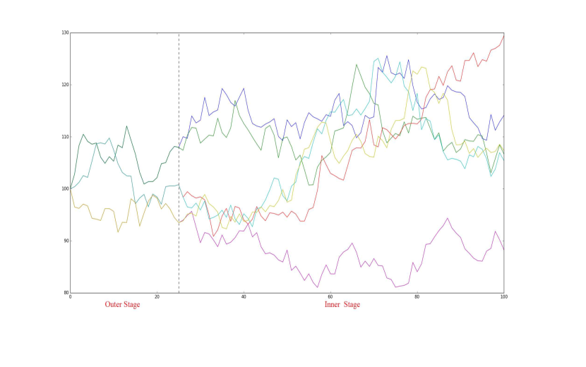
Figure 1: The two stage procedure: the $x$-axis is time, the $y$-axis is the stock price.

The common objective is measuring the risk of a portfolio of assets at the risk horizon $t=\tau$, while standing at time $0$. We denote the current wealth, i.e., the net present value of portfolio, by $X_{0}$ (a known quantity). At time $\tau$, the value of the portfolio is then a $\mathcal{F}_{\tau}$-measurable random variable $X_{\tau}$. In almost all real-world applications, we assume a probabilistic model of the evolution of uncertainty between $0$ and $\tau$, for example, a stochastic differential equation. Suppose the outcome $\varOmega$ is a set of possible future scenarios, each of which incorporates sufficient information so as to determine all asset prices at the risk horizon. Then, in each scenario $\omega\in\varOmega$, the portfolio has value $X_{\tau}(\omega)$. The mark-to-market (MTM) loss of this portfolio at time $\tau$ in scenario $\hat{\omega}\in\varOmega$ is given by

$$L(\hat{\omega})=X_{0}-X_{\tau}(\hat{\omega}).$$ (39)

The usual risk measurement is static in the sense that it evaluates the risk of exposure at risk horizon only at current time $0$. If one wants to check the risk at an intermediate point of the risk horizon, the whole model has to be re-run. Given the computation efforts of nested simulation, it can be very burdensome. In addition, re-simulating can cause inconsistency of risk evaluation, which is also undesired.

In our work, we use dynamic risk measure and the approximation algorithm (35) proposed in section 5, to measure the risk associated with the portfolio dynamically. In this way, the risk can be monitored continuously and consistently; in other words, for any time instant $t$ within the risk horizon, the evolution of risk can be traced.

To better illustrate the dynamic risk evaluation, let us consider a specific example, a portfolio consisting of a long position in a single vanilla put option, which expires at time $T$ and has strike price $K$. The underlying stock, say ABC, follows a geometric Brownian motion with an initial price $S_{0}$, mean $\mu$ and volatility $\sigma$; under the real-world probability measure $\mathbb{P}$, its dynamics is given by the following SDE:

$$\frac{dS_{t}}{S_{t}}=b\;dt+\sigma\;dW_{t},\quad t\in[0,T].$$ (40)

Here, $\{W_{t}\}$ is $\mathbb{P}$-Brownian motion. Let us also set a flat interest rate $r$; therefore, under the risk-neutral pricing framework, we have the stock dynamics:

$$\frac{dS_{t}}{S_{t}}=r\;dt+\sigma\;d\widetilde{W}_{t},$$ (41)

where $\widetilde{W}_{t}$ is a $\mathbb{Q}$-Brownian motion. With these specifications, the initial value of the put can be easily calculated by the Black-Scholes (BS) formula, which yields

$$\mathcal{P}(0,S_{0}):=\textit{BS}(0,S_{0},\sigma,K,T)=S_{0}N(d_{+}(T,S_{0}))-KD(0,T)N(d_{-}(T,S_{0}));$$

here $N$ stands for the standard normal cumulative distribution function and

$$d_{+}(\tau,x) =\frac{1}{\sigma\sqrt{\tau}}\big{[}\ln\frac{x}{K}+(r+{\textstyle{\frac{1}{2}}}\sigma^{2})\tau\big{]},$$

$$d_{-}(\tau,x) =\frac{1}{\sigma\sqrt{\tau}}\big{[}\ln\frac{x}{K}+(r-{\textstyle{\frac{1}{2}}}\sigma^{2})\tau\big{]}.$$

Let us fix a risk horizon $\tau$, denote the price at the risk horizon as $S_{\tau}(\omega)$. Then, the exposure (MTM) at time $\tau$ is the difference of initial put price $\mathcal{P}(0,S_{0})$ and the risk-neutral price of the option at time $\tau$, i.e.,

$$\varPhi(S_{\tau}(\omega)):=\mathcal{P}(0,S_{0})-\mathbb{E}^{\mathbb{Q}}\big{[}\,(S_{T}-K)^{+}\,\big{|}\,S_{\tau}(\omega)\big{]}.$$ (42)

Here, to get $S_{\tau}(\omega)$, we have to simulate the path of stock under the real-world measure, i.e., according to (40). Then, to compute the right-hand side, we only need to work out the second term; again, it can be computed analytically by the BS formula. It is well known that the loss function $\varPhi(\cdot)$ is Lipschitz in the state. We are now in the situation to apply a dynamic risk measure,

$$\rho_{t,\tau}^{g}\big{[}\,\varPhi(S_{\tau})\,\big{]}:=Y_{t},\quad\text{where}\quad Y_{t}=\varPhi(S_{\tau})+\int_{t}^{\tau}g(s,Z_{s})\;ds-\int_{t}^{\tau}Z_{s}\;dW_{s},\quad t\in[0,\tau],$$ (43)

which enables us to view the risk at any time $t\in[0,\tau]$.

As for the implementation details, instead of using Monte Carlo simulation, we use a tree model for the outer stage. Our risk evaluation algorithm (38) reduces the functional optimization to vector optimization at every time discretization step. However, since backward induction has to be implemented, the state space also needs to be discretized, which makes the tree structure appealing.

Remark 6.1.

For a diversified portfolio, we shall do a multi-dimensional outer loop simulations, because multiple assets are involved. Also, more sophisticated underlying dynamics is possible, such as stochastic volatility, local volatility model, in which cases Monte Carlo simulation has to be performed. At the risk horizon, all exposures should be netted before the $g$-evaluation by our algorithm for BSDEs.

We now present the numerical results based on the following data: $K=95$, $T=0.75$, $S_{0}=100$, $\mu=0.08$, $\sigma=0.2$, $r=0.03$, $\tau=0.2$. For the risk evaluation, we specify the driver to be:

$$g(z)=\gamma\|\max\{z\mathcal{N},0\}\|_{p},\quad\mathcal{N}\sim N(0,1),$$

where the parameters $\gamma>0$ and $p\geq 1$ model risk aversion. The corresponding dual set is then:

$$\mathcal{A}=\partial g(0)=\{\,l\in\mathbb{R}^{n}_{+}:|l|_{q}\leq\gamma k\,\},$$

with $1/p+1/q=1$, and

$$k=\begin{cases}\frac{1}{\sqrt{2}}(2m(2m-1)\cdots(m+1))^{\frac{1}{2m}},&\quad\text{if }p=2m,\\ (2^{m}\sqrt{2}\pi m!)^{\frac{1}{2m+1}},&\quad\text{if }p=2m+1.\\ \end{cases}$$

Fix $p=2$, at time $0$, given $\mathcal{F}_{\tau}$-measurable loss $\varPhi(\cdot)$ in (42). Table 1 and Figure 2 summarize the valuation when varying the step size and risk tolerance $\gamma$. We can observe convergence of the numerical method, as the step size decreases, uniformly over the whole range of $\gamma$.

Table 1: Risk Valuation Convergence Table

step size	$\gamma=0.1$	$\gamma=0.3$	$\gamma=0.4$	$\gamma=0.6$	$\gamma=0.8$	$\gamma=1.0$
0.4	0.00000	0.00000	0.00000	0.00000	0.00000	0.00000
0.2	0.03407	0.23907	0.34080	0.54207	0.73957	0.93217
0.1	0.06371	0.37300	0.52628	0.82895	1.12492	1.41239
0.08	0.07086	0.40174	0.56573	0.88956	1.20628	1.51403
0.05	0.08261	0.44695	0.62757	0.98446	1.33392	1.67410
0.04	0.08687	0.46282	0.64924	1.01771	1.37878	1.73064
0.02	0.09622	0.49671	0.69544	1.08872	1.47500	1.85268
0.01	0.10165	0.51579	0.72141	1.12877	1.52971	1.92284
0.008	0.10287	0.51998	0.72712	1.13760	1.54184	1.93852
0.005	0.10485	0.52674	0.73632	1.15187	1.56152	1.96407
0.004	0.10557	0.52919	0.73965	1.15705	1.56869	1.97344
0.002	0.10720	0.53465	0.74709	1.16864	1.58483	1.99465
0.001	0.10822	0.53798	0.75163	1.17574	1.59479	2.00786
0.0008	0.10845	0.53876	0.75269	1.17740	1.59713	2.01099
0.0005	0.10886	0.54007	0.75447	1.18021	1.60109	2.01630
0.0004	0.10901	0.54057	0.75515	1.18127	1.60260	2.01833

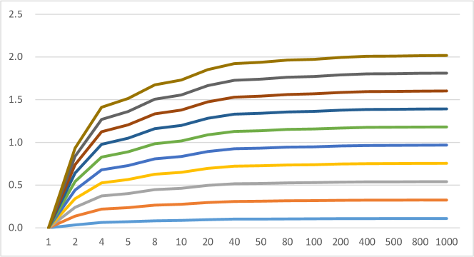
Figure 2: Convergence of the discretization method for $\gamma$ ranging from $0.1$ (bottom graph) to $1.0$ (top graph); the $x$-axis represents the number of time steps, while the $y$-axis is the risk estimate.

If we vary the underlying asset’s volatility as well as the strike price of the contract, we can construct the risk surface. As Table 2 and Figure 3 show, the risk is plotted against different combinations of volatility $\sigma$ and strike price $K$.

Table 2: Risk Surface Table

$K$, $\sigma$	0.1	0.3	0.5	0.6	0.7	0.8	0.9	1
70	-0.0002	-0.1479	-0.0901	0.0566	0.2612	0.5101	0.7918	1.0962
80	-0.0041	-0.0188	0.2444	0.4645	0.7290	1.0279	1.3517	1.6918
90	0.0737	0.3661	0.7508	1.0114	1.3099	1.6379	1.9869	2.3489
100	0.7941	1.0211	1.4004	1.6691	1.9782	2.3177	2.6780	3.0506
110	2.4089	1.8858	2.1561	2.4081	2.7100	3.0475	3.4087	3.7833
120	3.9179	2.8641	2.9802	3.2007	3.4842	3.8108	4.1655	4.5361
130	4.6752	3.8600	3.8387	4.0233	4.2831	4.5938	4.9376	5.3003

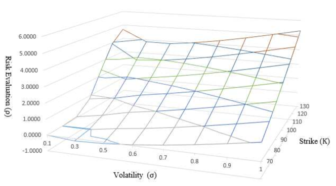
Figure 3: The dependence of risk on the strike price and volatility.

As we can observe, if the stock ABC becomes volatile, the risk of the portfolio should increase, because volatility implies uncertainty. Moreover, since the current stock price is $100$, as the strike price increases, the risk also goes up, which indicates being engaged in an out-of-money trade is riskier than at-the-money or in-the-money. Thus, the risk surface constructed coincides with intuition, which validates the risk evaluation approximation.

6.2 Risk-Averse Portfolio Pricing

We consider $n$ stock prices $\big{\{}S^{(i)}_{t}\big{\}}$, $i=1,\dots,n$, following the system of stochastic differential equations

$$\frac{dS^{(i)}_{t}}{S^{(i)}_{t}}=b^{(i)}\;dt+\sigma^{(i)}\;dW_{t},\quad t\in[0,T].$$ (44)

Here, $\{W_{t}\}$ is an $n$-dimensional Brownian motion, $b^{(i)}$ is the drift of stock $i$, and $\sigma^{(i)}$ is the $n$-dimensional (row) vector of volatility coefficients of stock $i$. For simplicity, we assume that these coefficients are constant, but nothing in our calculations hinges on that.

At time $T$, a random function $\varPhi(S_{T})$ is evaluated. In our example, it is the value of a portfolio of European call options, $\varPhi(S_{T})=\sum_{i=1}^{n}x_{i}\max\big{(}S_{T}^{(i)}-K^{(i)},0\big{)}$, where $x_{i}$ is the number of option $i$ held, and $K^{(i)}$ is the strike price. Of course, any other function of $S_{T}$ is possible here as well.

Let the risk free rate be $r$. Using the multi-dimensional Girsanov Theorem, we change the real-world probability measure $\mathbb{P}$ to the risk-neutral probability measure $\mathbb{Q}$, and the stock prices follow the system:

$$\frac{dS^{(i)}_{t}}{S^{(i)}_{t}}=r\;dt+\sigma^{(i)}\;d\widetilde{W}_{t},\quad t\in[0,T].$$ (45)

In this equation, $\widetilde{W}_{t}$ is an $n$-dimensional Brownian motion with independent components under $\mathbb{Q}$. All calculations are performed under $\mathbb{Q}$. The valuation equation is the BSDE:

$$Y_{t}=\varPhi(S_{T})+\int_{t}^{T}[-rY_{t}+g(Z_{\tau})]\;d\tau-\int_{t}^{T}Z_{\tau}\;d\widetilde{W}_{r},\quad t\in[0,T].$$ (46)

If $g\equiv 0$, this reduces to the standard arbitrage-free valuation:

$$Y_{t}=e^{-r(T-t)}\mathbb{E}^{\mathbb{Q}}\big{[}\varPhi(S_{T})\big{]},$$

but in the risk-averse case the BSDE (46) must be solved.

We first simulate the forward process (45). We apply $n$-dimensional symmetric random walk to approximate the independent Brownian motions. Specifically, we use binomial tree data structure in $n$ dimensions to monitor the stock prices at all lattice points at each discrete time step $t_{i}=i\Delta_{t}$, $i=0,1,2,\dots,N$, where $t_{N}=T$.

Having the terminal prices for all the stocks, it is easy to generate the terminal states for BSDE part. To evaluate the dynamic risk in the process, we set the driver $g(z)=\gamma\|z\|$, which satisfies the assumptions for the dual method. Here, $\gamma>0$ is the level of risk aversion. The corresponding dual set (subdifferential) is $A=\{{a}\;|\;\left\|{a}\right\|\leq\gamma\}$.

In our problem, $\rho^{g}_{0}[\varPhi(S_{T})]$ is the risk-adjusted price at time 0 for the seller, which means that the seller, given his risk aversion, is willing to sell the option at that price. On the other hand, $-\rho^{g}_{0}[-\varPhi(S_{T})]$ represents the risk-adjusted price at time 0 for the buyer. The prices are different, of course, because the risk measure is not linear: $-\rho^{g}_{0}[-\varPhi(S_{T})]<\rho^{g}_{0}[\varPhi(S_{T})]$.

In the dual method, at each node of the lattice, the optimization problem (38) was solved by the gradient method with projection (see, e.g. [40, Sec. 6.1.1]), which has an easy closed-form representation, due to the fact that $A$ is just a ball. The normal distribution was represented by the $2^{n}$ points of the $n$-dimensional random walk.

For comparison, we also used the $\theta$-method of [6], with $\theta=1/2$. Both methods were applied to evaluate the buyer’s price on an example with $n=d=5$ and

$$S_{0}=K=[50,60,70,80,90],\ r=0.03,\ \gamma=0.5,\ x=(0.2,0.2,0.2,0.2,0,2),$$

$$\sigma=\begin{bmatrix}0.1&0.2&0.3&-0.2&0.15\\ 0.3&0.1&-0.15&0.3&0.22\\ 0.2&0.15&0.2&0.5&0.1\\ 0.1&0.3&0.2&-0.1&0.05\\ -0.13&0.3&0.1&0.1&-0.15\end{bmatrix}.$$

The results are depicted in Figure 4. The horizontal axis is the number of discretization points $N$.

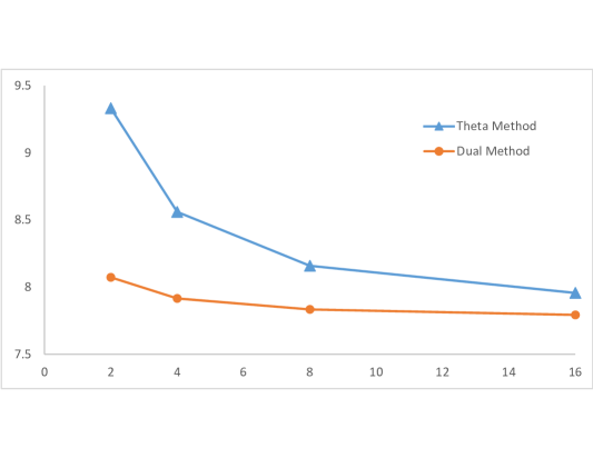
Figure 4: Convergence of the Dual Method (lower graph) and the $\theta$-Method (upper graph) for the buyer, when $\gamma$ = 0.5.

.

We can see from the figure that the dual method exhibits much faster convergence than the $\theta$-method. This is due to the fact that it exploits the convexity of the driver in the dual optimization step (38), thus minimizing the numerical error accumulated.

The results have been borrowed from extensive tests carried out in [22] for the buyer’s and seller’s prices for several examples with different dimensions and different risk aversion coefficient $\gamma$. In all experiments reported there, the pattern is very similar to Figure 4: the dual method significantly outperforms the $\theta$-method. We believe that for convex drivers, the dual method is a very attractive numerical approach to backward stochastic differential equations.

References

- [1] Artzner, P. and Delbaen, F. and Eber, J. M. and Heath, D., Thinking Coherently, RISK, volume 10, 68-71, 1997.
- [2] Artzner, P. and Delbaen, F. and Eber,J. M. and Heath, D. Coherent Measures of Risk, Mathematical Finance, volume 9, 203-228, 1999.
- [3] Barrieu, P. and El Karoui, N., Optimal derivatve design under dynamic risk measures, Mathematics of Finance, Contemporary Mathematics, volume 351, 13-26, 2004.
- [4] Barrieu, P. and El Karoui, N., Pricing, hedging and optimally designing derivatives via minimization of risk measures, Volume on Indifference Pricing, Princeton University Press, 2009.
- [5] J. Bion-Nadal, Dynamic risk measures: time consistency and risk measures from bmo martingales, Finance and Stochastics, 12:219–244, 2008.
- [6] Bouchard, B., Touzi, N., Discrete-time approximation and Monte Carlo simulation of backward stochastic differential equations, Stochastic Processes and Their Applications, 111(2):175-206. 2004.
- [7] Briand, P., B. Delyon, and J. Mémin, On the robustness of backward stochastic differential equations, Stochastic Processes and their Applications, 97:229–253, 2002.
- [8] P. Cheridito, F. Delbaen, and M. Kupper, Dynamic monetary risk measures for bounded discrete-time processes, Electronic Journal of Probability, 11:57–106, 2006.
- [9] P. Cheridito and M. Kupper, Composition of time-consistent dynamic monetary risk measures in discrete time, International Journal of Theoretical and Applied Finance, 14(1):137–162, 2011.
- [10] Coquet, F., Hu, Y., Mémin, J., and Peng, S., Filtration-consistent nonlinear expectations and related g-expectations, Probability Theory and Related Fields, volume 123, 1-27, 2002.
- [11] Delbaen, F., Peng, S., and Rosazza Gianin, E., Representation of the penalty term of dynamic concave utilities, Finance and Stochastics, 14(3):449–472, 2010.
- [12] Detlefsen, K., Scandolo, G., Conditional and Dynamic Convex Risk Measures, Finance and Stochastics, volume 9, 539-561, 2005.
- [13] H. Föllmer and I. Penner, Convex risk measures and the dynamics of their penalty functions, Statistics and Decisions, 24:61–96, 2006.
- [14] Föllmer, H. and Schied, A., Convex measures of risk and trading constraints, Finance and Stochastic, volume 6, 429-447, 2002.
- [15] Föllmer, H. and Schied, A., Stochastic Finance: An Introduction in Discrete Time, 2nd ed, De Gruyter Berlin, 2004
- [16] Fritelli, M., Rosazza Gianin, E., Putting Order in Risk Measures, Math. Finance, volume 16, 589-612, 2006.
- [17] M. Fritelli and Scandolo, G., Risk measures and capital requirements for processes, Math. Finance, 16:589–612, 2006.
- [18] Gobet, E., Lemor, J.-P., and Warin, X., A regression-based Monte Carlo method to solve backward stochastic differential equations, The Annals of Applied Probability 15.3 (2005): 2172-2202.
- [19] Gobet, E., and Turkedjiev, P., Linear regression MDP scheme for discrete backward stochastic differential equations under general conditions, Mathematics of Computation, 85(299), 1359-1391, 2016.
- [20] Gordy, M.B., Juneja, S., Nested simulation in portfolio risk measurement, Federal Reserve Board, FEDS 2008-2-21, 2008.
- [21] Henry-Labordere, P., Tan, X., and Touzi, N., A numerical algorithm for a class of BSDEs via the branching process, Stochastic Processes and their Applications, 124(2), 1112-1140, 2014.
- [22] Hu, Y., Ni, B., Ruszczyński, A., Yao, J., Numerical Methods for Forward-Backward Stochastic Differential Equations with Application to Risk-Averse Option Portfolio Valuation, technical report, Rutgers University, November, 2018.
- [23] Ikeda, N., and Watanabe, S., Stochastic Differential Equations and Diffusion Processes, Kodansha, Tokyo 1981.
- [24] Kloeden, P.E., Platen, E., Numerical Solution of Stochastic Differential Equations, Springer, Berlin, 1992.
- [25] Laeven, R. J. A., Stadje, M., Robust portfolio choice and indifference valuation, Mathematics of Operations Research, 39(4):1109–1141, 2014.
- [26] Lee, S.H., Glynn, P.W., Computing the distribution function of a conditional expectation via Monte Carlo simulation: discrete conditioning spaces, ACM Transactions on Modeling and Computer Simulation, 13(3), 235-258, 2002.
- [27] Lesnevski, V., Nelson, B.L., Staum, J., Simulation of coherent risk measures, Proceedings of the 2004 Winter Simulation Conference, 1579-1585, 2004.
- [28] Lesnevski, V., Nelson, B.L., Staum, J., Simulation of coherent risk measures based on generalized scenarios, Management Science, 53(11), 1756-1769, 2007.
- [29] Ludwig, S., Sirignano, J., Huang, R., and Papanicolaou, G., A Forward-Backward Algorithm For Stochastic Control Problems, SciTePress, 83-89, 2012.
- [30] Ma, J., Protter, P., and Douglas, J. Numerical methods for forward-backward stochastic differential equations, Annals of applied probability, 6(3): 940 - 968, 1996.
- [31] Ma, J., Protter, P., Martin, J., and Torres, S., Numerical Method For Backward Stochastic Differential Equations, Annals of Applied Probability, volume 12, 302-316, 2002.
- [32] Ma, J., and Yong, J., Forward-backward stochastic differential equations and their applications. No. 1702. Springer Science & Business Media, 1999.
- [33] Nualart, D., The Malliavin Calculus and Related Topics, Springer, 2006.
- [34] Øksendal, B., and Sulem, A., Maximum Principles For Optimal Control Of Forward-Backward Stochastic Differential Equations With Jumps, SIAM Journal Control Optimization, volume 48, 2945-2976, 2009.
- [35] Peng, S., Nonlinear expectations, nonlinear evaluations and risk measures, Lecture Notes in Mathematics, Springer, 2004.
- [36] Pardoux,E. and Peng,S., Adapted solutions of backward stochastic differential equation, System and Control Letters, volume 14, 55-61, 1990.
- [37] Quenez, M.-C., and Sulem, A., BSDEs with jumps, optimization and applications to dynamic risk measures, Stochastic Processes and their Applications, 123(8):3328–3357, 2013.
- [38] Riedel, F., Dynamic coherent risk measures, Stochastic Processes and their Applications, 112:185–200, 2004.
- [39] Rockafellar, R.T., Uryasev, S., Conditional value-at-risk for general loss distributions, Journal of Banking and Finance, 26, 1443- 1471, 2002.
- [40] A. Ruszczyński. Nonlinear Optimization, Princeton University Press, 2006.
- [41] Ruszczyński, A., Risk-averse dynamic programming for Markov decision processes, Mathematical Programming Series B, volume 125, 235-261, 2010.
- [42] Ruszczyński, A. and Shapiro, A., Optimization of convex risk functions, Mathematics of Operations Research, volume 31, 433-542, 2006.
- [43] Ruszczyński, A. and Shapiro, A., Conditional Risk Mapping, Mathematics of Operations Research, volume 31, 544-561, 2006.
- [44] Ruszczyński, A., Yao, J., A Risk-Averse Analog of the Hamilton-Jacobi-Bellman Equation, SIAM Control and Its Application Conference Proceedings, 2015.
- [45] Shapiro, A., Dentcheva, D.,and Ruszczyński, A., Lectures on Stochastic Programming. Modeling and Theory, SIAM-Society for Industrial and Applied Mathematics, Philadelphia, 2009.
- [46] Stadje, M., Extending Dynamic Convex Risk Measures From Discrete Time to Continuous Time: a Convergence Approach, Insurance: Mathematics and Economics, volume 47, 391-404, 2010.
- [47] Yong, J., and Zhou, X. Y., Stochastic Controls: Hamiltonian Systems and HJB Equations, Springer-Verlag, New York, 1999.
- [48] Zhang, J., Some Fine Properties of Backward Stochastic Differential Equations, with Applications, Ph.D. dissertation, Purdue University, (2001).
- [49] Zhang, J., Numerical Method For Backward Stochastic Differential Equations, Annals of Applied Probability, volume 14, 459-488, 2004.
- [50] Zhang, J., Backward Stochastic Differential Equations, Springer, New York, 2017.