Martingale optimal transport with stopping

Abstract.

We solve the martingale optimal transport problem for cost functionals represented by optimal stopping problems. The measure-valued martingale approach developed in [6] allows us to obtain an equivalent infinite-dimensional controller-stopper problem. We use the stochastic Perron’s method and characterize the finite dimensional approximation as a viscosity solution to the corresponding HJB equation. It turns out that this solution is the concave envelope of the cost function with respect to the atoms of the terminal law. We demonstrate the results by finding explicit solutions for a class of cost functions.

1. Introduction

The aim of this article is to solve a class of martingale optimal transport problems for which the cost functional can be represented as an optimal stopping problem of the underlying cost function. Specifically, given a continuous and bounded cost function $f:\nobreak\mathbb{R}\to\mathbb{R}$ we are interested in solving the martingale optimal transport problem

$$\sup_{P_{\mu}}P^{\mathbb{P}}(f)\quad\text{with}\quad P^{\mathbb{P}}(f)=\sup_{\tau\in\mathcal{T}_{0}}\mathbb{E}[f(M_{\tau})].$$ (1.1)

The outer supremum is taken over $P_{\mu}$ - the set of all pairs of filtered probability spaces $(\Omega,\mathcal{F},(\mathcal{F}_{t})_{t\geq 0},\mathbb{P})$ and continuous martingales $M=(M_{t})_{t\geq 0}$ on them such that the filtration $(\mathcal{F}_{t})_{t\geq 0}$ is generated by a Brownian motion and the terminal law is $M_{T}\sim\mu$ under $\mathbb{P}$. The inner stopping problem is over $\mathcal{T}_{s}$ - the set of all $(\mathcal{F}_{t})$-stopping times taking values in $[s,T]$ for $s\in[0,T]$ and some fixed terminal time $T>0$.

The duality between martingale optimal transport and robust pricing problems was studied in a related setting in Dolinsky and Soner [8] for general path-dependent European-type cost functionals (i.e. payoffs) and continuous models. Recently Bayraktar and Miller [1] and Beiglböck et al. [5] obtained solutions to distribution-constrained optimal stopping problems by using dynamic programming and martingale transport methods, respectively. In contrast to our setting, however, the constraints in [1] and [5] are on the distribution of the stopping times and not on the marginal distribution at the terminal time. By using the concept of measure-valued martingales Cox and Kallbläd [6] studied the robust pricing of Asian-type options subject to a marginal distribution constraint. The authors cast the original problem into a control theoretic framework and obtained a viscosity characterization of the solution.

Here we employ the control theoretic approach of [6] and [1] to analyze optimal martingale transport problems with cost functionals which are of American type. The difficulty in our setting is that we have an additional optimal stopping component. However, the fact that we optimize over continuous models allows us to prove that the resulting value function is time-independent up to the terminal time. Since the original problem is infinite dimensional we use the continuity with respect to the terminal law to restrict it only to measures with finitely many atoms. Working in a Brownian filtration allows us to recast this finite dimensional approximation as a recursive sequence of controller-stopper problems with exit-time components. We prove that the value functions of these problems are viscosity solutions to the corresponding sequence of elliptic obstacle problems satisfying exact Dirichlet boundary conditions. We achieve this by applying the stochastic Perron’s approach in the spirit of Bayraktar and Sirbu [4] where the obstacle problems are associated with Dynkin games and Rokhlin [14] where an elliptic Dirichlet boundary problem arose from exit-time stochastic control. We circumvent the potential difficulty of proving a strong comparison result for viscosity sub/supersolutions satisfying generalized boundary conditions (see [14]) by using the recursive structure of the problem to show the exact attainment of these boundary conditions.

The main result in this paper, Theorem 3.1, is the characterization of the value function of the finite dimensional martingale transport problem as the concave envelope of the pay-off with respect to the probability weights of the terminal law’s atoms. In this final step we use a recent result of Oberman and Ruan [11] on characterizing convex envelopes as unique viscosity solutions to obstacle problems with appropriate Dirichlet boundary conditions. One possible application of our results is the robust pricing of American options. Indeed, the martingales over which we optimize can be seen as different models for the stock price with a given marginal distribution at the terminal time.

The rest of the paper is organized as follows: In Section 2, we formulate the finite dimensional approximation of the Martingale Optimal Transport problem, see (2.12). In Section 3, we employ the stochastic Perron’s method to characterize the value function as the unique viscosity solution of the corresponding Dirichlet obstacle problem and to show its concave envelope form in an appropriate phase space. Section 4 illustrates how our results can be achieved in a probabilistic framework and provides concrete examples.

2. Problem formulation

We define the set of measures $\mathcal{P}$ as

$$\mathcal{P}:=\{\mu\in\mathcal{B}(\mathbb{R}_{+}):\mu(\mathbb{R}_{+})=1\text{ and }\int|x|\mu(dx)<\infty\},$$

and suppose that the terminal law $\mu$ of the martingales in the optimal transport problem (1.1) satisfies $\mu\in\mathcal{P}$. In the usual optimal transport framework we can regard the probability measures $\mathbb{P}$ contained in $P_{\mu}$ as transporting the initial Dirac measure $\delta_{M_{0}}$ (i.e. the law of $M_{0}$) to the terminal law $\mu$ under the cost functional $P^{\mathbb{P}}$ - both of these laws are known at time $t=0$. On the other hand, notice that the continuous martingale $M$ satisfies

$$M_{t}=\mathbb{E}[M_{T}|\mathcal{F}_{t}]=\int x\,\xi_{t}(dx)\quad\text{for}\quad t\in[0,T],$$ (2.1)

where $\xi_{t}$ is the conditional law of $M_{T}$ given $\mathcal{F}_{t}$ under the measure $\mathbb{P}$. In particular, we have that $\xi_{0}=\mu$ and $\xi_{T}=\delta_{M_{T}}$. Therefore, similarly to the method proposed in [6], we can rewrite (1.1) in its measure-valued martingale formulation as

$$\sup_{(\xi_{t})\in\Xi}\sup_{\tau\in\mathcal{T}_{0}}\mathbb{E}[f(M_{\tau})]\quad\text{subject to}\quad\xi_{0}=\mu,$$ (2.2)

where $\Xi$ is the set of all terminating measure-valued (i.e. $\mathcal{P}$-valued) martingales (see Definition 2.7 in [6]) such that $(\int x\,\xi_{t}(dx))_{t\geq 0}$ is a continuous process a.s. with respect to the filtered probability space $(\Omega,\mathcal{F},(\mathcal{F}_{t})_{t\geq 0},\mathbb{P})$ for all $(\xi_{t})_{t\geq 0}\in\Xi$, where $(\mathcal{F}_{t})_{t\geq 0}$ is a Brownian filtration. Moreover, as in [6], we fix the probability space $(\Omega,\mathcal{F},(\mathcal{F}_{t})_{t\geq 0},\mathbb{P})$ which does not materially change our conclusions.

Let us write (2.2) in the Markovian form

$$U(t,\xi)=\sup_{(\xi_{r})\in\Xi}\sup_{\tau\in\mathcal{T}_{t}}\mathbb{E}[f(M_{\tau})|\xi_{t}=\xi],$$ (2.3)

and note that we have the following variant of Lemma 3.1 in [6] the proof of which can be found in the appendix:

Lemma 2.1.

If $f$ is non-negative and Lipschitz then the function $U$ is continuous in $\xi$ (in the Wasserstein-1 topology) and independent of $t$ for $t\in[0,T)$.

The continuity in $\xi$ allows us to apply the finite dimensional reduction from Section 3.2 in [6]. In particular, we introduce the set $\mathbb{X}_{N}=\{x_{0},\dots,x_{N}\}$ where $0\leq x_{0}<x_{1}<\dots<x_{N}$ and let $\mathcal{P}^{N}=\mathcal{P}\cap\mathcal{M}(\mathbb{X}_{N})$ and $\mathcal{P}(\mathbb{X}_{\alpha})=\mathcal{P}\cap\mathcal{M}(\mathbb{X}_{\alpha})$ for any $\alpha\subseteq\{0,1,\dots,N\}$, where $\mathcal{M}(\mathbb{X}_{N})$ resp. $\mathcal{M}(\mathbb{X}_{\alpha})$ denote the sets of all measures on $\mathbb{X}_{N}$ resp. $\mathbb{X}_{\alpha}:=\{x_{i}:i\in\alpha\}$. We assume from now on that the terminal law $\xi$ (i.e. also $\mu$) is an atomic measure and satisfies $\xi\in\mathcal{P}^{N}$. Since we work in a Brownian filtration, by martingale representation for any terminating $\mathcal{P}^{N}$-valued martingale $(\xi_{t})_{t\geq 0}$ it is true that the (nonnegative) martingales $\xi^{n}_{t}:=\xi_{t}(\{x_{n}\})$ solve an SDE of the form

$$d\xi^{n}_{t}=w^{n}_{t}dW_{t}$$ (2.4)

for $t\geq 0$ and $n=0,\dots,N$, where the vector of weights $\mathbf{w}_{t}=(w_{t}^{0},\dots,w_{t}^{N})$ satisfies $\sum_{n=0}^{N}w_{t}^{n}=0$, and $\xi^{n}_{t}\in\{0,1\}$ implies that $w^{n}_{t}=0$. The following result, by analogy to Corollary 3.6 in [6], follows directly from Lemma 3.4 in [6] and allows us to work with a bounded set of controls:

Lemma 2.2.

Under the above assumption that $\mu\in\mathcal{P}^{N}$, the value function in (2.3) for $t\in[0,T)$ reduces to the value function

$$V(\xi)=\sup_{\mathbf{w}\in\mathcal{A}}\sup_{\tau\in\mathcal{T}_{0}}\mathbb{E}\left[f\left(\sum_{j=0}^{N}x_{j}\,\xi^{j}_{T^{-1}_{\tau}}\right)|\xi_{0}=\xi\right],$$ (2.5)

where the admissible control set $\mathcal{A}$ is defined as

$$\mathcal{A}:=\{(\mathbf{w}_{r})_{r\geq 0}\text{ prog. meas.}:\mathbf{w}_{r}\in\operatorname*{cl}(\mathbb{D}^{N+1})\,,\,\xi^{n}_{r}\in\{0,1\}\text{ implies }w^{n}_{r}=0\},$$

with the disk $\mathbb{D}^{k+1}$ being the intersection of the open unit ball with the hyperplane $z_{1}+\dots+z_{k+1}=0$ in $\mathbb{R}^{k+1}$, and $T^{-1}_{r}$ is the continuous inverse of

$$T_{r}:=\int_{0}^{r}\lambda_{s}ds\quad\text{for}\quad r\geq 0,$$ (2.6)

where the strictly positive time change rate process $\lambda=(\lambda_{r})_{r\geq 0}$ satisfies

$$\lVert{\mathbf{w}}_{r}\rVert^{2}+\lambda_{r}=1-I_{\{\xi_{r}=\delta_{x_{i}}\}}I_{\{T_{r}=T\}}.$$ (2.7)

The role of the time change in (2.6) is to stretch/compress the original time scale so as to bound the volatility of the state process (i.e. the control process $\mathbf{w}$). Thus we avoid technical difficulties arising from unbounded control sets later when proving the viscosity characterization of the value function.

Now notice that the value function $V(\xi)$ can be identified with $\tilde{V}_{N}(\xi)$ where for $k=1,\dots,N$, and $\xi\in\mathcal{P}(\mathbb{X}_{\alpha})$, with $|\alpha|=k+1$, we introduce the sequence of problems

$$\tilde{V}_{k}(\xi)=\sup_{\mathbf{w}\in\mathcal{A}^{\alpha}}\sup_{\tau\in\mathcal{T}_{0}}\mathbb{E}\Big{[} \tilde{V}_{k-1}(\xi_{\sigma})I_{\{T_{\sigma}\leq\tau\}}+f\Big{(}\sum_{j=0}^{N}x_{j}\,\xi^{j}_{T^{-1}_{\tau}}\Big{)}I_{\{T_{\sigma}>\tau\}}|\xi_{0}=\xi\Big{]},$$ (2.8)

with

$$\mathcal{A}^{\alpha} :=\{(\mathbf{w}_{r})_{r\geq 0}\text{ prog. meas.}:\mathbf{w}_{r}\in\operatorname*{cl}(\mathbb{D}^{N+1})\,,$$ (2.9)

$$\phantom{:=\{(\mathbf{w}_{r})_{r\geq 0}\text{ prog. meas.}:\,\,}\,w^{i}\equiv 0\text{ for any }i\in\{0,1,\dots,N\}\setminus\alpha\},$$

$$\sigma :=\inf\{s\geq 0:\xi_{s}\in\mathcal{P}(\mathbb{X}_{\alpha^{\prime}})\text{ for some }\alpha^{\prime}\text{ with }|\alpha^{\prime}|\leq k\text{ or }T_{s}=T\},$$ (2.10)

and $\tilde{V}_{0}(\xi)=f(x_{i})$ for $\xi=\delta_{x_{i}}$. From now on we will denote the time changed filtration as $(\mathcal{G}_{t})_{t\geq 0}:=(\mathcal{F}_{T_{t}})_{t\geq 0}$ and suppress its dependence on $\lambda$ for notational purposes. The following lemma shows that we can ignore controls which are small enough and that we can work with stopping times in the time changed filtration.

Lemma 2.3.

The value function $\tilde{V}_{k}(\xi)$ can be written as

$$\tilde{V}_{k}(\xi)=\sup_{\mathbf{w}\in\operatorname*{int}(\mathcal{A}^{\alpha}_{\varepsilon})}\sup_{\tau\in\mathcal{T}}\mathbb{E}\Big{[} \tilde{V}_{k-1}(\xi_{\sigma})I_{\{\sigma\leq\tau\}}+f\Big{(}\sum_{j=0}^{N}x_{j}\,\xi^{j}_{\tau}\Big{)}I_{\{\sigma>\tau\}}|\xi_{0}=\xi\Big{]},\!\!$$ (2.11)

where $\operatorname*{int}(\mathcal{A}_{\varepsilon}^{\alpha}):=\{(\mathbf{w}_{r})_{r\geq 0}\in\mathcal{A}^{\alpha}:\mathbf{w}_{r}\in\mathbb{D}^{N+1},\;\xi_{r}\neq\delta_{x_{i}}\text{ implies }\lVert\mathbf{w}_{r}\rVert\geq\varepsilon\}$ for any $\varepsilon\in[0,1)$ and $\mathcal{T}$ is the set of all $(\mathcal{G}_{t})$-stopping times for an appropriately time changed filtration $(\mathcal{G}_{t})_{t\geq 0}$.

Proof.

For any time change rate $\lambda$ we have $\lambda_{u}>0$ for $u\geq 0$ and from (2.7) it follows that $\lVert\mathbf{w}_{u}\rVert<1$. Moreover, since $\lambda$ is strictly positive, we have that $T_{r}$ and $T^{-1}_{t}$ are strictly increasing. It follows immediately that if $\tau\in[0,T]$ is an $(\mathcal{F}_{t})$-stopping time then $T^{-1}_{\tau}\geq 0$ is a $(\mathcal{G}_{t})$-stopping time and, conversely, if $\tau\geq 0$ is a $(\mathcal{G}_{t})$-stopping time then $T_{\tau}\in[0,T]$ is an $(\mathcal{F}_{t})$-stopping time. Therefore in (2.8) we can substitute $\mathcal{T}_{0}$ with $\mathcal{T}$ and $\tau$ with $T_{\tau}$.

What is left is to prove that we can take the outer supremum in (2.8) over $\operatorname*{int}(\mathcal{A}^{\alpha}_{\varepsilon})\subset\operatorname*{int}(\mathcal{A}^{\alpha})$. For $0<\varepsilon<1$ and any $\mathbf{w}\in\operatorname*{int}(\mathcal{A}^{\alpha})\setminus\operatorname*{int}(\mathcal{A}_{\varepsilon}^{\alpha})$ we can choose $\tilde{\mathbf{w}}\in\operatorname*{int}(\mathcal{A}_{\varepsilon}^{\alpha})$ defined as $\tilde{\mathbf{w}}^{n}_{s}:=\sqrt{\bar{\varepsilon}_{s}}\mathbf{w}^{n}_{\phi(s)}$ where

$$\phi(s)=\int_{0}^{s}\bar{\varepsilon}_{u}du\quad\text{with}\quad\bar{\varepsilon}_{s}=\frac{\varepsilon^{2}}{\lVert\mathbf{w}_{\phi(s)}\rVert^{2}},$$

and $\phi(s)$ is the right-continuous inverse of the (non-strictly) increasing continuous function $\phi^{-1}(s)$ given by

$$\phi^{-1}(s)=\int_{0}^{s}\frac{\lVert\mathbf{w}_{u}\rVert^{2}}{\varepsilon^{2}}du.$$

From (2.4) we see that $\xi^{n}_{r}$ (corresponding to the control $\mathbf{w}$) has the same distribution as $\tilde{\xi}^{n}_{\phi^{-1}(r)}$ (corresponding to the control $\tilde{\mathbf{w}}$). Hence, for any $(\mathcal{G}_{t})$-stopping time $\tau$ we have that $\tilde{\tau}=\phi^{-1}(\tau)$ is a $(\mathcal{G}_{\phi(t)})$-stopping time such that $\xi^{n}_{\tau}$ has the same law as $\tilde{\xi}^{n}_{\tilde{\tau}}$. We conclude from (2.8). ∎

Before going further we introduce some additional notation. Let $\alpha(\xi)$ be the subset of elements in $\mathbb{X}_{N}$ to which the atomic measure $\xi\in\mathcal{P}^{N}$ prescribes nonzero probability and notice that we have the consistency conditions

$$\tilde{V}_{k}(\xi)=\tilde{V}_{|\alpha(\xi)|-1}(\xi)\quad\text{for}\quad k\geq|\alpha(\xi)|.$$

For every $\xi\in\mathcal{P}^{N}$ with $|\alpha(\xi)|=k+1$ it is true that $\xi=\sum_{j=0}^{k}\xi^{i_{j}}\delta_{x_{i_{j}}}$ where $\alpha(\xi)=\{x_{i_{0}},\dots,x_{i_{k}}\}\subseteq\mathbb{X}_{N}$. Hence, we can identify every $\xi\in\mathcal{P}^{N}$ with the vector $\xi^{\alpha}:=(\xi^{i_{0}},\xi^{i_{1}},\dots,\xi^{i_{k}})\in\operatorname*{int}(\Delta^{k+1})$ where $\alpha=\{i_{0},\dots,i_{k}\}$ and $\Delta^{k+1}:=\{\mathbf{z}\in\mathbb{R}_{\geq 0}^{k+1}:\sum z_{i}=1\}$. We let

$$V_{\alpha}(\xi^{\alpha})=\tilde{V}_{|\alpha(\xi)|-1}(\xi),\quad\bar{f}(\xi^{\alpha})=f(\mathbf{x}^{\alpha}\cdot\xi^{\alpha}),$$ (2.12)

where $\mathbf{x}^{\alpha}:=(x_{i_{0}},\dots,x_{i_{k}})$. For any $r\geq 0$ and $\mathbf{w}=(w^{0},\dots,w^{N})\in\operatorname*{int}(\mathcal{A}^{\alpha})$ we also let $\bm{\xi}^{\mathbf{w},r,\xi^{\alpha}}_{u}:=(\xi^{i_{0},w^{i_{0}},r}_{u},\xi^{i_{1},w^{i_{1}},r}_{u},\dots,\xi^{i_{k},w^{i_{k}},r}_{u})$, where $\xi^{i_{j},w^{i_{j}},r}_{u}$ is the unique strong solution to (2.4) with control $w^{i_{j}}$ and initial condition $\xi^{i_{j},w^{i_{j}},r}_{u}=\xi^{i_{j}}$ for $u\leq r$. Denote by $\xi^{\mathbf{w},r,\xi^{\alpha}}$ the $\mathcal{P}^{N}$-valued martingale corresponding to $\bm{\xi}^{\mathbf{w},r,\xi^{\alpha}}$, i.e. $\xi^{\mathbf{w},r,\xi^{\alpha}}_{u}:=\sum_{j=0}^{k}\xi^{i_{j},w^{i_{j}},r}_{u}\delta_{x_{i_{j}}}$. For short we let $\bm{\xi}^{\mathbf{w},\xi^{\alpha}}:=\bm{\xi}^{\mathbf{w},0,\xi^{\alpha}}$ and $\xi^{\mathbf{w},\xi^{\alpha}}:=\xi^{\mathbf{w},0,\xi^{\alpha}}$.

3. Viscosity characterization of the value function using stochastic Perron’s method

We want to obtain the viscosity characterization of the value function $V_{\alpha}$. Fix $0<c<1$ and $\alpha\subseteq\{0,\dots,N\}$ with $|\alpha|=k+1\geq 2$ for some integer $k\geq 1$. Using (2.12) rewrite the value function from (2.11) as

$$V_{\alpha}(\xi^{\alpha}) =\sup_{\mathbf{w}\in\operatorname*{int}(\mathcal{A}^{\alpha}_{c})}\sup_{\tau\in\mathcal{T}}\mathbb{E}\left[\tilde{V}_{k-1}(\xi^{\mathbf{w},r,\xi^{\alpha}}_{\sigma})I_{\{\sigma\leq\tau\}}+\bar{f}(\bm{\xi}^{\mathbf{w},r,\xi^{\alpha}}_{\tau})I_{\{\sigma>\tau\}}\right],$$ (3.1)

where $\xi^{\alpha}\in\Delta^{k+1}$. Our aim is to show that $V_{\alpha}$ is the unique viscosity solution (see e.g. Definition 7.4 in [7]) to the associated Dirichlet obstacle problem given by

$$\min\Big{\{}-\sup_{\mathbf{w}\in\mathbb{D}^{k+1}_{c}}\frac{1}{2}\operatorname*{tr}(\mathbf{w}\mathbf{w}^{\prime}D_{\bm{\xi}}^{2}V_{\alpha}),V_{\alpha}-\bar{f}\Big{\}} =0\quad\text{on}\quad\operatorname*{int}(\Delta^{k+1}),$$ (3.2)

$$\!\!V_{\alpha}(\xi^{\alpha}) =g(\xi^{\alpha}):=V_{\alpha^{\prime}}(\xi^{\alpha^{\prime}})\quad\text{on}\quad\partial\Delta^{k+1},\!$$ (3.3)

where $\xi^{\alpha^{\prime}}$ and $\alpha^{\prime}$ correspond to the nonzero components of $\xi^{\alpha}$ and $\alpha$, and $\mathbb{D}^{k+1}_{c}:=\nobreak\{\mathbf{w}\in\mathbb{D}^{k+1}:\lVert\mathbf{w}\rVert>c\}$. The derivative $D_{\bm{\xi}}^{2}$ is to be understood in the directional sense - i.e. we restrict ourselves to second directional derivatives $\operatorname*{tr}(\mathbf{w}\mathbf{w}^{\prime}D_{\bm{\xi}}^{2})$ w.r.t. directions lying in the set $\mathbb{D}^{k+1}_{c}$.

We are now ready to state the main result of the paper - its proof relies on the stochastic Perron’s method and we present it in the next section.

Theorem 3.1.

The function $V_{\alpha}:\Delta^{k+1}\to\mathbb{R}$ defined in (3.1) is the unique continuous viscosity solution of the obstacle problem (3.2) satisfying the Dirichlet boundary condition (3.3). Moreover, $V_{\alpha}$ is the concave envelope of $\bar{f}$ on $\Delta^{k+1}$ - i.e. denoting the projection of $\Delta^{k+1}$ onto $\mathbb{R}_{\geq 0}^{k}$ by $\tilde{\Delta}^{k}$ and the projected functions $\tilde{V}_{\alpha},\tilde{f}:\tilde{\Delta}^{k}\to\mathbb{R}$ as

$$\tilde{V}_{\alpha}(z_{0},\dots,z_{k-1}):=V_{\alpha}\Big{(}z_{0},\dots,z_{k-1},1-\sum_{i=1}^{k-1}z_{i}\Big{)},$$ (3.4)

$$\tilde{f}(z_{0},\dots,z_{k-1}):=\bar{f}\Big{(}z_{0},\dots,z_{k-1},1-\sum_{i=1}^{k-1}z_{i}\Big{)},$$ (3.5)

the function $\tilde{V}_{\alpha}$ is the concave envelope of $\tilde{f}$.

3.1. Proof of Theorem 3.1

We begin by introducing the notions of stochastic sub- and supersolutions.

Definition 3.1.

The set of stochastic subsolutions to the PDE (3.2) with the boundary condition (3.3), denoted by ${\mathcal{V}}^{-}$, is the set of functions $v:\Delta^{k+1}\to\mathbb{R}$ that have the following properties:

1. They are continuous and bounded, and satisfy the boundary condition

   $$v(\xi^{\alpha})\leq g(\xi^{\alpha})\quad\text{on}\quad\partial\Delta^{k+1}.$$ (3.6)

2. For each $\tau\in\mathcal{T}$ and $\bm{\xi}\in\mathcal{G}_{\tau}$ with $\mathbb{P}(\bm{\xi}\in\Delta^{k+1})=1$ there exists a control $\mathbf{w}\in\operatorname*{int}(\mathcal{A}^{\alpha})$ such that for any $\rho\in\mathcal{T}$ with $\rho\in[\tau,\sigma(\tau,\bm{\xi},\mathbf{w})]$ we have a.s. that

   $$v(\bm{\xi})\leq\mathbb{E}[v(\bm{\xi}^{\mathbf{w},\tau,\bm{\xi}}_{\rho\wedge\tau_{*}(v)})|\mathcal{G}_{\tau}],$$ (3.7)

   where the $(\mathcal{G}_{t})$-stopping times $\sigma(\tau,\bm{\xi},\mathbf{w})$ and $\tau_{*}(v)$ are defined as

   $$\sigma(\tau,\bm{\xi},\mathbf{w}):=\inf\{s\geq\tau:\bm{\xi}^{\mathbf{w},\tau,\bm{\xi}}_{s}\notin\operatorname*{int}(\Delta^{k+1})\},$$ (3.8)

   $$\tau_{*}(v)\equiv\tau_{*}(v;\tau,\bm{\xi},\mathbf{w}):=\inf\{s\geq\tau:v(\bm{\xi}^{\mathbf{w},\tau,\bm{\xi}}_{s})\leq\bar{f}(\bm{\xi}^{\mathbf{w},\tau,\bm{\xi}}_{s})\}.$$ (3.9)

Definition 3.2.

The set of stochastic supersolutions to the PDE (3.2) with the boundary condition (3.3), denoted by ${\mathcal{V}}^{+}$, is the set of functions $v:\Delta^{k+1}\to\mathbb{R}$ that have the following properties:

1. They are continuous and bounded, and satisfy the boundary condition

   $$v(\xi^{\alpha})\geq g(\xi^{\alpha})\quad\text{on}\quad\partial\Delta^{k+1}.$$ (3.10)

2. For each $\tau\in\mathcal{T}$ and $\bm{\xi}\in\mathcal{G}_{\tau}$ with $\mathbb{P}(\bm{\xi}\in\Delta^{k+1})=1$, for any control $\mathbf{w}\in\operatorname*{int}(\mathcal{A}^{\alpha}_{c})$ and any $\rho\in\mathcal{T}$ with $\rho\in[\tau,\sigma(\tau,\bm{\xi},\mathbf{w})]$ we have a.s. that

   $$v(\bm{\xi})\geq\mathbb{E}[v(\bm{\xi}^{\mathbf{w},\tau,\bm{\xi}}_{\rho})|\mathcal{G}_{\tau}],$$ (3.11)

   where $\sigma(\tau,\bm{\xi},\mathbf{w})$ is defined as in (3.8).

Clearly ${\mathcal{V}}^{-}$ (resp. ${\mathcal{V}}^{+}$) is nonempty since $\bar{f}$ is bounded from below (resp. above) and any constant which is small (large) enough belongs to ${\mathcal{V}}^{-}$ (resp. ${\mathcal{V}}^{+}$). Actually, we can easily verify that $\bar{f}\in{\mathcal{V}}^{-}$. The following lemma proves an important property of the sets ${\mathcal{V}}^{-}$ and ${\mathcal{V}}^{+}$.

Lemma 3.1.

For any two $v^{1},v^{2}\in{\mathcal{V}}^{-}$ we have that $v^{1}\vee v^{2}\in{\mathcal{V}}^{-}$. For any two $v^{1},v^{2}\in{\mathcal{V}}^{+}$ we have that $v^{1}\wedge v^{2}\in{\mathcal{V}}^{+}$.

Proof.

We will only prove the first part of the lemma - the second part follows in a similar way. Denote $v=v^{1}\vee v^{2}$ and notice that item (i) in Definition 3.1 is clearly satisfied by $v$. Now fix $\tau\in\mathcal{T}$ and $\bm{\xi}\in\mathcal{G}_{\tau}$ as in item (ii) of Definition 3.1 and introduce the sequence of stopping time, control and state process triples $(\gamma_{n},\mathbf{w}^{n},\bm{\xi}^{n})_{n\geq-1}$ defined recursively as follows:

$$(\gamma_{-1},\mathbf{w}^{-1},\bm{\xi}^{-1})\equiv(\gamma_{0},\mathbf{w}^{0},\bm{\xi}^{0}):=(\tau,\mathbf{1}_{\{v^{1}(\bm{\xi})\geq v^{2}(\bm{\xi})\}}\mathbf{w}^{0,1}+\mathbf{1}_{\{v^{1}(\bm{\xi})<v^{2}(\bm{\xi})\}}\mathbf{w}^{0,2},\bm{\xi}^{{\mathbf{w}}^{0},\tau,\bm{\xi}})$$

where $\mathbf{w}^{0,1},\mathbf{w}^{0,2}$ are the controls corresponding to the stochastic subsolutions $v^{1},v^{2}$ starting at the pair $(\tau,\bm{\xi})$, and for $n=0,1,2\dots$:

1. if $v(\bm{\xi}^{n}_{\gamma_{n}})\leq\bar{f}(\bm{\xi}^{n}_{\gamma_{n}})$ then we set

   $$(\gamma_{n+1},\mathbf{w}^{n+1},\bm{\xi}^{n+1}):=(\gamma_{n},\mathbf{w}^{n},\bm{\xi}^{n}).$$

2. if $v(\bm{\xi}^{n}_{\gamma_{n}})=v^{i}(\bm{\xi}^{n}_{\gamma_{n}})>\bar{f}(\bm{\xi}^{n}_{\gamma_{n}})$ for $i\in\{1,2\}$ then we set

   $$\gamma_{n+1}:=\sigma(\gamma_{n},\bm{\xi}^{n}_{\gamma_{n}},\mathbf{w}^{n})\wedge\tau_{*}(v^{i};\gamma_{n},\bm{\xi}^{n}_{\gamma_{n}},\mathbf{w}^{n})$$

   $$\mathbf{w}^{n+1}:=\mathbf{w}^{n+1,i},\quad\bm{\xi}^{n+1}:=\bm{\xi}^{\mathbf{w}^{n+1,i},\gamma_{n+1},\bm{\xi}^{n}_{\gamma_{n+1}}},$$

   where $\mathbf{w}^{n+1,i}$ is the control process corresponding to the stochastic subsolution $v^{i}$ starting at the pair $(\gamma_{n+1},\bm{\xi}^{n}_{\gamma_{n+1}})$, and $\tau_{*}(v^{i};\gamma_{n},\bm{\xi}^{n}_{\gamma_{n}},\mathbf{w}^{n})$ is defined as in (3.9).

Define the control $\mathbf{w}$ by

$$\mathbf{w}_{s}:=\sum_{n=1}^{\infty}\mathbf{1}_{\{s\in[\gamma_{n},\gamma_{n+1})\}}\mathbf{w}^{n}_{s}$$

and notice that by construction $\bm{\xi}^{n}_{s}=\bm{\xi}^{\mathbf{w},\tau,\bm{\xi}}_{s}$ for $s\in[\gamma_{n},\gamma_{n+1}]$ and any $n\geq 0$. For any stopping time $\rho\in\nobreak[\tau,\sigma(\tau,\bm{\xi},\mathbf{w})]$ denote $\rho\wedge\gamma_{n}=\rho_{n}$. By the definition of the sequence $(\gamma_{n},\mathbf{w}^{n},\bm{\xi}^{n})$ we get that

$$v(\bm{\xi}^{n}_{\rho_{n}})=(\mathbf{1}_{\{v^{1}\geq v^{2}\}}v^{1}+\mathbf{1}_{\{v^{1}<v^{2}\}}v^{2})(\bm{\xi}^{n}_{\rho_{n}})$$

$$\leq\mathbb{E}[(\mathbf{1}_{\{v^{1}(\bm{\xi}^{n}_{\rho_{n}})\geq v^{2}(\bm{\xi}^{n}_{\rho_{n}})\}}v^{1}+\mathbf{1}_{\{v^{1}(\bm{\xi}^{n}_{\rho_{n}})<v^{2}(\bm{\xi}^{n}_{\rho_{n}})\}}v^{2})(\bm{\xi}^{n+1}_{\rho_{n+1}})|\mathcal{G}_{\rho_{n}}]$$

$$\leq\mathbb{E}[v(\bm{\xi}^{n+1}_{\rho_{n+1}})|\mathcal{G}_{\rho_{n}}],$$

and by iterating the above we conclude that

$$v(\xi)\leq\mathbb{E}[v(\bm{\xi}^{n+1}_{\rho_{n+1}})|\mathcal{G}_{\tau}]=\mathbb{E}[v(\bm{\xi}^{\mathbf{w},\tau,\bm{\xi}}_{\rho_{n+1}})|\mathcal{G}_{\tau}],$$ (3.12)

for any $n\geq 0$. Now we apply the same reasoning as in the proof of Lemma 2.3 in [4] to conclude that

$$\lim_{n\to\infty}\gamma_{n}=\sigma(\tau,\bm{\xi},\mathbf{w})\wedge\tau_{*}(v;\tau,\bm{\xi},\mathbf{w})\quad a.s.$$

By taking $n\to\infty$ in (3.12) and using the bounded convergence theorem we finally obtain that $v$ satisfies (3.7) and, hence, is a stochastic subsolution. ∎

We introduce the assumption:

Assumption 3.1.

The boundary function $g$ is continuous on $\partial\Delta^{k+1}$.

Proposition 3.1.

Under Assumption 3.1 the lower stochastic envelope $v^{-}:=\sup_{v\in{\mathcal{V}}^{-}}v\leq V_{\alpha}$ is a viscosity supersolution and the upper stochastic envelope $v^{+}:=\inf_{v\in{\mathcal{V}}^{+}}v\geq V_{\alpha}$ is a viscosity subsolution of (3.2) and (3.3).

Proof.

The proof uses ideas from Theorem 3.1 (and Theorem 4.1) in [3] and Theorem 2 in [14]. We repeat the key steps for the lower stochastic envelope $v^{-}$.

Denote for short $V\equiv V_{\alpha}$. It is clear that $v^{-}\leq V$ since in item (ii) of Definition 3.1 we can choose $\tau=0$, a constant $\bm{\xi}\in\Delta^{k+1}$ and $\rho=\sigma(\tau,\bm{\xi},\mathbf{w})$ for some control $\mathbf{w}\in\operatorname*{int}(\mathcal{A}^{\alpha})$, and use the condition (3.6) and (3.9).

We will prove the viscosity supersolution property of $v^{-}$ by contradiction. Take a $C^{2}$ test function $\varphi:\Delta^{k+1}\to\mathbb{R}$ such that $v^{-}-\varphi$ achieves a strict local minimum equal to 0 at some boundary point $\xi_{0}\in\partial\Delta^{k+1}$ (the case when $\xi_{0}\in\operatorname*{int}(\Delta^{k+1})$ is simpler). Assume that $v^{-}$ is not a viscosity supersolution and hence

$$\max\big{\{}(-\sup_{\mathbf{w}\in\mathbb{D}^{k+1}_{c}}L^{\mathbf{w}}\varphi)(\xi_{0}),(\varphi-g)(\xi_{0})\big{\}}<0,$$

where

$$(L^{\mathbf{w}}\varphi)(\xi):=\frac{1}{2}\operatorname*{tr}(\mathbf{w}\mathbf{w}^{\prime}D_{\bm{\xi}}^{2}\varphi(\xi)).$$

It follows that there exists $\tilde{\mathbf{w}}\in\mathbb{D}^{k+1}_{c}$ such that

$$(-L^{\tilde{\mathbf{w}}}\varphi)(\xi_{0})<0.$$ (3.13)

By the continuity of $\varphi$, $g$ and the lower semicontinuity of $v^{-}$ we can find a small enough open ball $B(\xi_{0},\varepsilon)$ and a small enough $\delta>0$ such that

$$(-L^{\tilde{\mathbf{w}}}\varphi)(\xi)<0,\quad\xi\in B(\xi_{0},\varepsilon)\cap\Delta^{k+1},$$

$$\varphi<g,\quad\text{on}\quad B(\xi_{0},\varepsilon)\cap\partial\Delta^{k+1},$$

$$\varphi(\xi)<v^{-}(\xi),\quad\xi\in B(\xi_{0},\varepsilon)\cap\Delta^{k+1}\setminus\{\xi_{0}\},$$

$$v^{-}-\delta\geq\varphi\quad\text{on}\quad(\overline{B(\xi_{0},\varepsilon)}\setminus B(\xi_{0},\varepsilon/2))\cap\Delta^{k+1}.$$

Using Proposition 4.1 in [2] together with Lemma 3.1 above, we obtain an increasing sequence of stochastic subsolutions $v_{n}\in{\mathcal{V}}^{-}$ with $v_{n}\nearrow v^{-}$. In particular, since $\varphi$ and the $v_{n}$’s are continuous we can use an argument identical to the one in Lemma 2.4 in [4] to obtain for any fixed $\delta^{\prime}\in(0,\delta)$ a corresponding $v=v_{n}\in{\mathcal{V}}^{-}$ such that

$$v-\delta^{\prime}\geq\varphi\quad\text{on}\quad(\overline{B(\xi_{0},\varepsilon)}\setminus B(\xi_{0},\varepsilon/2))\cap\Delta^{k+1}.$$

Now we can choose $\eta\in(0,\delta^{\prime})$ small enough such that $\varphi^{\eta}:=\varphi+\eta$ satisfies

$$(-L^{\tilde{\mathbf{w}}}\varphi^{\eta})(\xi)<0,\quad\xi\in B(\xi_{0},\varepsilon)\cap\Delta^{k+1},$$

$$\varphi^{\eta}<g,\quad\text{on}\quad B(\xi_{0},\varepsilon)\cap\partial\Delta^{k+1},$$

$$\varphi^{\eta}<v\quad\text{on}\quad(\overline{B(\xi_{0},\varepsilon)}\setminus B(\xi_{0},\varepsilon/2))\cap\Delta^{k+1}.$$

We define

$$v^{\eta}=\begin{cases}v\vee\varphi^{\eta}\;&\text{on}\;\overline{B(\xi_{0},\varepsilon)}\cap\Delta^{k+1},\\ v&\text{otherwise},\end{cases}$$

and notice that $v^{\eta}$ is continuous and $v^{\eta}(\xi_{0})=v^{-}(\xi_{0})+\eta>v^{-}(\xi_{0})$. Since condition (3.6) clearly also holds, we see that $v^{\eta}$ satisfies item (i) of Definition 3.1. What is left is to check item (ii) in Definition 3.1 and obtain $v^{\eta}\in{\mathcal{V}}^{-}$ which will lead to a contradiction since $v^{\eta}(\xi_{0})>v^{-}(\xi_{0})$.

Choose $\tau\in\mathcal{T}$ and $\bm{\xi}\in\mathcal{G}_{\tau}$ with $\mathbb{P}(\bm{\xi}\in\Delta^{k+1})=1$, and, similarly to the proof of Lemma 3.1 above, introduce the sequence of stopping time, control and state process triples $(\gamma_{n},\mathbf{w}^{n},\bm{\xi}^{n})_{n\geq-1}$ defined recursively as follows:

$$(\gamma_{-1},\mathbf{w}^{-1},\bm{\xi}^{-1})\equiv(\gamma_{0},\mathbf{w}^{0},\bm{\xi}^{0}):=(\tau,\tilde{\mathbf{w}}\mathbf{1}_{A}+\bar{\mathbf{w}}^{0}\mathbf{1}_{A^{c}},\bm{\xi}^{{\mathbf{w}}^{0},\tau,\bm{\xi}}),$$

where $\bar{\mathbf{w}}^{0}$ is the control corresponding to the stochastic subsolution $v$ starting at the pair $(\tau,\bm{\xi})$, the event $A$ is given by

$$A=A(\bm{\xi}):=\{\bm{\xi}\in B(\xi_{0},\varepsilon/2)\cap\Delta^{k+1}\text{ and }\varphi^{\eta}(\bm{\xi})>v(\bm{\xi})\}$$

and for $n=0,1,2\dots$:

1. if $v^{\eta}(\bm{\xi}^{n}_{\gamma_{n}})\leq\bar{f}(\bm{\xi}^{n}_{\gamma_{n}})$ then we set

   $$(\gamma_{n+1},\mathbf{w}^{n+1},\bm{\xi}^{n+1}):=(\gamma_{n},\mathbf{w}^{n},\bm{\xi}^{n}).$$

2. if $A(\bm{\xi}^{n}_{\gamma_{n}})$ holds then we set

   $$\gamma_{n+1}:=\sigma(\gamma_{n},\bm{\xi}^{n}_{\gamma_{n}},\mathbf{w}^{n})\wedge\tau_{1}(\gamma_{n},\bm{\xi}^{n}_{\gamma_{n}},\mathbf{w}^{n})\wedge\tau_{*}(\varphi^{\eta};\gamma_{n},\bm{\xi}^{n}_{\gamma_{n}},\mathbf{w}^{n}),$$

   $$\mathbf{w}^{n+1}:=\tilde{\mathbf{w}},\quad\bm{\xi}^{n+1}:=\bm{\xi}^{\tilde{\mathbf{w}},\gamma_{n+1},\bm{\xi}^{n}_{\gamma_{n+1}}},$$

   where the $\mathcal{G}_{t}$-stopping time $\tau_{1}$ is defined by

   $$\tau_{1}(\tau,\bm{\xi},\mathbf{w}):=\inf\{s\geq\tau:\bm{\xi}^{\mathbf{w},\tau,\bm{\xi}}_{s}\in\partial B(\xi_{0},\varepsilon/2)\},$$

   and $\tau_{*}$ is defined as in (3.9).

3. otherwise we set

   $$\gamma_{n+1}:=\sigma(\gamma_{n},\bm{\xi}^{n}_{\gamma_{n}},\mathbf{w}^{n})\wedge\tau_{*}(v;\gamma_{n},\bm{\xi}^{n}_{\gamma_{n}},\mathbf{w}^{n})$$

   $$\bm{\xi}^{n+1}:=\bm{\xi}^{\mathbf{w}^{n+1},\gamma_{n+1},\bm{\xi}^{n}_{\gamma_{n+1}}},$$

   where $\mathbf{w}^{n+1}$ is the control process corresponding to the stochastic subsolution $v$ starting at the pair $(\gamma_{n+1},\bm{\xi}^{n}_{\gamma_{n+1}})$.

By construction we have that $\gamma_{n}\leq\tau_{*}(v^{\eta};\tau,\bm{\xi},\mathbf{w})$ where the control $\mathbf{w}\in\operatorname*{int}(\mathcal{A}^{\alpha}_{c})$ is defined as

$$\mathbf{w}_{s}:=\sum_{n=1}^{\infty}\mathbf{1}_{\{s\in[\gamma_{n},\gamma_{n+1})\}}\mathbf{w}^{n}_{s}.$$

Introduce the event

$$B:=\{\gamma_{n}<\tau_{*}(v^{\eta};\tau,\bm{\xi},\mathbf{w})\wedge\sigma(\tau,\bm{\xi},\mathbf{w})\quad\text{for all }n\in\mathbb{N}\}$$

and notice that for each $\omega\in B$ there exists $n_{0}(\omega)$ such that

$$\varphi^{\eta}(\bm{\xi}^{n_{0}+2l+1}_{\gamma_{n_{0}+2l+1}})\leq\bar{f}(\bm{\xi}^{n_{0}+2l+1}_{\gamma_{n_{0}+2l+1}})$$ (3.14)

$$\qquad\text{ if }\tau_{*}(\varphi^{\eta};\gamma_{n_{0}+2l},\bm{\xi}^{n_{0}+2l}_{\gamma_{{n_{0}+2l}}},\mathbf{w}^{n_{0}+2l})<\tau_{1}(\gamma_{n_{0}+2l},\bm{\xi}^{n_{0}+2l}_{\gamma_{{n_{0}+2l}}},\mathbf{w}^{n_{0}+2l}),$$

$$v^{\eta}(\bm{\xi}^{n_{0}+2l+1}_{\gamma_{n_{0}+2l+1}})=v(\bm{\xi}^{n_{0}+2l+1}_{\gamma_{n_{0}+2l+1}})$$ (3.15)

$$\qquad\text{ if }\tau_{*}(\varphi^{\eta};\gamma_{n_{0}+2l},\bm{\xi}^{n_{0}+2l}_{\gamma_{{n_{0}+2l}}},\mathbf{w}^{n_{0}+2l})\geq\tau_{1}(\gamma_{n_{0}+2l},\bm{\xi}^{n_{0}+2l}_{\gamma_{{n_{0}+2l}}},\mathbf{w}^{n_{0}+2l}),$$

$$v(\bm{\xi}^{n_{0}+2l+1}_{\gamma_{n_{0}+2l+1}})\leq\bar{f}(\bm{\xi}^{n_{0}+2l+1}_{\gamma_{n_{0}+2l+1}}),$$ (3.16)

for $l\geq 0$. Denoting $\gamma_{\infty}:=\lim_{n}\gamma_{n}$ and noticing that $\bm{\xi}^{{\mathbf{w}},\tau,\bm{\xi}}_{s}=\bm{\xi}^{n}_{s}$ for $s\in\nobreak[\gamma_{n},\gamma_{n+1})$ we take the limit in (3.16) to obtain

$$v(\bm{\xi}^{{\mathbf{w}},\tau,\bm{\xi}}_{\gamma_{\infty}})\leq\bar{f}(\bm{\xi}^{{\mathbf{w}},\tau,\bm{\xi}}_{\gamma_{\infty}}).$$ (3.17)

Now assume there exists $C\subseteq B$ such that for each $\omega\in C$ we have

$$\varphi^{\eta}(\bm{\xi}^{{\mathbf{w}},\tau,\bm{\xi}}_{\gamma_{\infty}})>\bar{f}(\bm{\xi}^{{\mathbf{w}},\tau,\bm{\xi}}_{\gamma_{\infty}}),$$

and conclude from (3.14)-(3.15) that there exists large enough positive integer $M(\omega)$ such that for all $n\geq M$ we have

$$v^{\eta}(\bm{\xi}^{n}_{\gamma_{n}})=v(\bm{\xi}^{n}_{\gamma_{n}}).$$

By taking $n\to\infty$ above we get $v^{\eta}(\bm{\xi}^{{\mathbf{w}},\tau,\bm{\xi}}_{\gamma_{\infty}})=v(\bm{\xi}^{{\mathbf{w}},\tau,\bm{\xi}}_{\gamma_{\infty}})$ on $C$. Hence, by using (3.17) we see that

$$v^{\eta}(\bm{\xi}^{{\mathbf{w}},\tau,\bm{\xi}}_{\gamma_{\infty}})\leq\bar{f}(\bm{\xi}^{{\mathbf{w}},\tau,\bm{\xi}}_{\gamma_{\infty}})$$

on $C$. On the other hand, on $B\setminus C$ we have

$$\varphi^{\eta}(\bm{\xi}^{{\mathbf{w}},\tau,\bm{\xi}}_{\gamma_{\infty}})\leq\bar{f}(\bm{\xi}^{{\mathbf{w}},\tau,\bm{\xi}}_{\gamma_{\infty}})$$

and again from (3.17) we get

$$v^{\eta}(\bm{\xi}^{{\mathbf{w}},\tau,\bm{\xi}}_{\gamma_{\infty}})\leq\bar{f}(\bm{\xi}^{{\mathbf{w}},\tau,\bm{\xi}}_{\gamma_{\infty}})$$

on $B\setminus C$. It follows that $\gamma_{\infty}\geq\tau_{*}(v^{\eta};\tau,\bm{\xi},\mathbf{w})$ on $B$ and from the definition of $B$ we conclude that $\gamma_{\infty}=\tau_{*}(v^{\eta};\tau,\bm{\xi},\mathbf{w})\wedge\sigma(\tau,\bm{\xi},\mathbf{w})$.

Now take any $\rho\in\mathcal{T}$ with $\rho\in[\tau,\sigma(\tau,\bm{\xi},\mathbf{w})]$, let $\rho\wedge\gamma_{n}=\rho_{n}$ and notice that, by Itô’s formula applied to $\varphi^{\eta}$ and the subsolution property of $v$, we have

$$v^{\eta}(\bm{\xi}^{n}_{\rho_{n}})=(\mathbf{1}_{A}\varphi^{\eta}+\mathbf{1}_{A^{c}}v)(\bm{\xi}^{n}_{\rho_{n}})$$

$$\leq\mathbb{E}[(\mathbf{1}_{A(\bm{\xi}^{n}_{\rho_{n}})}\varphi^{\eta}+\mathbf{1}_{A(\bm{\xi}^{n}_{\rho_{n}})^{c}}v)(\bm{\xi}^{n+1}_{\rho_{n+1}})|\mathcal{G}_{\rho_{n}}]\leq\mathbb{E}[v^{\eta}(\bm{\xi}^{n+1}_{\rho_{n+1}})|\mathcal{G}_{\rho_{n}}],$$

and by iterating the above we conclude that

$$v(\bm{\xi})\leq\mathbb{E}[v(\bm{\xi}^{n+1}_{\rho_{n+1}})|\mathcal{G}_{\tau}]=\mathbb{E}[\bm{\xi}^{\mathbf{w},\tau,\bm{\xi}}_{\rho_{n+1}})|\mathcal{G}_{\tau}].$$ (3.18)

By taking $n\to\infty$ in (3.18) and using the bounded convergence theorem we obtain that $v^{\eta}$ satisfies item (ii) in Definition 3.1 Hence $v^{\eta}\in{\mathcal{V}}^{-}$ and we obtain contradiction and consequently the supersolution property of $v^{-}$. ∎

Assumption 3.2.

The boundary function $g$ is the concave envelope of $\bar{f}$ on the simplex faces $\{\mathbf{z}\in\Delta^{k+1}:z_{j}=0\}$ for all $j=0,\dots,k+1$.

Proposition 3.2.

Under Assumption 3.2 we have that $v^{-}=v^{+}=g$ on $\partial\Delta^{k+1}$.

Proof.

Let $\overline{v}$ be the concave envelope of $\bar{f}$ on the whole of $\Delta^{k+1}$. From Assumption 3.2 it follows that $\overline{v}=g$ on $\partial\Delta^{k+1}$ and $\overline{v}$ satisfies item (i) of Definition 3.2. Now take any $\tau\in\mathcal{T}$, $\bm{\xi}\in\mathcal{G}_{\tau}$ with $\mathbb{P}(\bm{\xi}\in\Delta^{k+1})=1$, $\mathbf{w}\in\operatorname*{int}(\mathcal{A}^{\alpha}_{c})$ and $\rho\in\mathcal{T}$ with $\rho\in[\tau,\sigma(\tau,\bm{\xi},\mathbf{w})]$, and notice that, by the Itô-Tanaka formula (see e.g. Theorem VI.1.5 in [13]) applied to the concave function $\overline{v}$ we have

$$\mathbb{E}[\overline{v}(\bm{\xi}^{\mathbf{w},\tau,\bm{\xi}}_{\rho})|\mathcal{G}_{\tau}]=\mathbb{E}[\overline{v}(\bm{\xi})+\int_{\tau}^{\rho}\overline{v}^{\prime}(\bm{\xi}^{\mathbf{w},\tau,\bm{\xi}}_{s})d\bm{\xi}^{\mathbf{w},\tau,\bm{\xi}}_{s}+\int_{\Delta^{k+1}}L_{\rho}^{a}\,\overline{v}^{\prime\prime}(da)|\mathcal{G}_{\tau}]\leq\overline{v}(\bm{\xi}),$$

where $\overline{v}^{\prime}$ is the left derivative, the second derivative $\overline{v}^{\prime\prime}$ is understood in the sense of a negative measure and $L^{a}$ is the local time at $a$ of the process $\bm{\xi}^{\mathbf{w},\tau,\bm{\xi}}$. Hence, item (ii) of Definition 3.2 is also satisfied and $\overline{v}$ is a stochastic supersolution. Since $v^{+}$ satisfies (3.10) and $v^{+}\leq\overline{v}$ it follows that $v^{+}=g$ on $\partial\Delta^{k+1}$.

Fix a constant control $\mathbf{w}\in\operatorname*{int}(\mathcal{A}^{\alpha}_{c})$ and define the function $\underline{v}:\Delta^{k+1}\to\mathbb{R}$ by

$$\underline{v}(\xi^{\alpha}) =\sup_{\bar{\tau}\in\mathcal{T}}\mathbb{E}\left[\tilde{V}_{k-1}(\xi^{\mathbf{w},\xi^{\alpha}}_{\sigma})I_{\{\sigma\leq\bar{\tau}\}}+\bar{f}(\bm{\xi}^{\mathbf{w},\xi^{\alpha}}_{\bar{\tau}})I_{\{\sigma>\bar{\tau}\}}\right].$$ (3.19)

The continuity of $\underline{v}(\xi^{\alpha})$ follows from the boundedness of the control $\mathbf{w}$ and standard results on optimal stopping problems (see e.g. Theorem 3.1.5 in [9]). We have that $\underline{v}(\xi^{\alpha})=V_{\alpha^{\prime}}(\xi^{\alpha^{\prime}})=g(\xi^{\alpha})$ for $\xi^{\alpha}\in\partial\Delta^{k+1}$ and we obtain that item (i) of Definition 3.1 is satisfied. Moreover, the optimal stopping time in (3.19) exists and is equal to $\tau^{*}=\sigma\wedge\tau_{*}(\underline{v};0,\xi^{\alpha},\mathbf{w})$ and it follows that $\underline{v}(\bm{\xi}^{\mathbf{w},\xi^{\alpha}}_{t\wedge\tau^{*}})$ is a martingale (see e.g. Theorems I.2.4 and I.2.7 in [12]). This means that (3.7) is satisfied with equality and $\underline{v}$ is a stochastic subsolution. By definition we know that $v^{-}\leq g$ on $\partial\Delta^{k+1}$ and $\underline{v}\leq v^{-}$. Hence, we conclude that $v^{-}=g$ on $\partial\Delta^{k+1}$. ∎

Proof of Theorem 3.1.

It is clear that if $|\alpha|=1$ then $V_{\alpha}(\xi^{\alpha})=\bar{f}(\xi^{\alpha})$ where $\xi=\delta_{x_{i}}$ for some $i$ and $\xi^{\alpha}=1$. We continue by induction and assume that we have proven the statement for all $k^{\prime}<k$. By the induction hypothesis $V_{\alpha^{\prime}}(\xi^{\alpha^{\prime}})$ is the concave envelope of $\bar{f}$ on the corresponding to $\alpha^{\prime}$ simplex face and hence Assumption 3.2 is satisfied. Moreover, value functions coincide on the intersection of their corresponding simplex faces, and therefore Assumpton 3.1 is also satisfied. Define the Hamiltonian $H$ as

$$H(A):=-\sup_{\mathbf{w}\in\mathbb{D}^{k+1}_{c}}\frac{1}{2}\operatorname*{tr}(\mathbf{w}\mathbf{w}^{\prime}A)\quad\text{for}\quad A\in\mathbb{R}^{(k+1)\times(k+1)},$$

and notice that for small enough $c$ the set $\mathbb{D}^{k+1}_{c}$ contains all directions in $\mathbb{R}^{k}$. On the other hand, $V_{\alpha}$ is a viscosity solution to (3.2) on $\operatorname*{int}(\Delta^{k+1})$ if and only if the projected function $\tilde{V}_{\alpha}$ defined in (3.4) is a viscosity solution of

$$\min\Big{\{}-\sup_{\mathbf{w}\in\tilde{\mathbb{D}}^{k}_{c}}\frac{1}{2}\operatorname*{tr}(\mathbf{w}\mathbf{w}^{\prime}D_{\bm{\xi}}^{2}\tilde{V}_{\alpha}),\tilde{V}_{\alpha}-\tilde{f}\Big{\}}=0$$ (3.20)

on $\operatorname*{int}(\tilde{\Delta}^{k})$, where $\tilde{\mathbb{D}}^{k}_{c}$ is the projection of $\mathbb{D}^{k+1}_{c}$ onto $\mathbb{R}^{k}$. Hence, the function $V_{\alpha}$ is a viscosity solution to $H(D_{\bm{\xi}}^{2}V_{\alpha})\geq 0$ if and only if $\tilde{V}_{\alpha}$ is a viscosity solution to $-\lambda_{k}[\tilde{V}_{\alpha}]\geq 0$, where $\lambda_{k}[\tilde{V}_{\alpha}]$ is the largest eigenvalue of the Hessian $D_{\bm{\xi}}^{2}\tilde{V}_{\alpha}$. Therefore we can apply Theorem 1 in [10] to obtain that any continuous viscosity solution to (3.20) is concave. Moreover, uniqueness of the solution to (3.20) together with the projected boundary condition

$$\tilde{V}_{\alpha}(\xi^{\alpha}) =\tilde{V}_{\alpha^{\prime}}(\xi^{\alpha^{\prime}}),$$ (3.21)

follows from the comparison principle for Dirichlet problems stated in Theorem 2.10 of [11]. This leads to uniqueness and comparison principle for our original problem (3.2)-(3.3). In particular, by Propositions 3.1 and 3.2 we have that $v^{+}\leq v^{-}$ on $\operatorname*{int}(\Delta^{k+1})$. On the other hand, by Proposition 3.1 we also have $v^{-}\leq V_{\alpha}\leq v^{+}$ on $\Delta^{k+1}$. Therefore, we can conclude that $v^{-}=V_{\alpha}=v^{+}$ on $\Delta^{k+1}$ and $V_{\alpha}$ is the unique viscosity solution of (3.2) with the boundary condition (3.3), and the same is true for the projected versions.

Finally, from Theorem 2 in [10] we have that the concave envelope of the projected cost function $\tilde{f}$ solves (3.20), and since it also clearly satisfies (3.21) we conclude from the uniqueness that $\tilde{V}_{\alpha}$ is the concave envelope of $\tilde{f}$. ∎

Remark 3.1.

The value function $V_{\alpha}$ can be regarded as the concave envelope on the simplex $\Delta^{k+1}$ of the modified cost function $\bar{f}$. Indeed, we can ignore one direction in the state space vector $\bm{\xi}$ due to the fact that $\Delta^{k+1}$ is a k-dimensional simplex and any concave function on a k-dimensional simplex in $\mathbb{R}^{k+1}$ is concave in any $k$ of its variables (and vice versa). Note that the optimal control weight vector $\mathbf{w}^{*}$ may not be unique. It is determined by the direction on the simplex $\Delta^{k+1}$ for which the second directional derivative of the value function $V_{\alpha}$ is zero - if the value function is linear at a point then clearly many directions satisfy this condition.

Remark 3.2.

When applying the stochastic Perron method to controlled exit time problems one needs a comparison result for the corresponding PDE in order to characterize the value function as a viscosity solution (see e.g. Definition 2 and Remark 1 in [14]). These comparison results are of a slightly different nature than the standard ones of e.g. Theorems 7.9 and 8.2 in [7] - the latter require an apriori knowledge of the behaviour of the stochastic semisolutions at the boundary. We were able to exploit the specific structure of our exit time problem in Proposition 3.2 to obtain the behaviour at the boundary of the stochastic semisolutions. This allowed the application of the comparison result in [11].

4. Examples

Let us first provide some intuition behind the choice of optimal controls and stopping times. We will consider a general class of cost functions - namely all bounded, non-negative Lipschitz continuous functions $f:\nobreak\mathbb{R}\to\mathbb{R}$. This is the class for which Theorem 3.1 holds. We will use our concave envelope characterization to choose the optimal controls and verify that Brownian exit times are optimal.

We abuse notation and regard $\bar{f}$ as a function on the projected set of probability vectors $\tilde{\Delta}^{N}:=\{\mathbf{z}\in\mathbb{R}_{\geq 0}^{N}:\sum z_{i}\leq 1\}$. Denote by $\operatorname*{conc}(\bar{f})$ the concave envelope of $\bar{f}$ on $\tilde{\Delta}^{N}$. For any initial probability vector $z\in\tilde{\Delta}^{N}$ corresponding to some terminal law $\mu$, e.g.

$$\mu=\sum_{i=1}^{N}z_{i}\delta_{x_{i}}+(1-\sum_{i=1}^{N}z_{i})\delta_{x_{0}},$$

we will find a candidate optimal control weight process $(\mathbf{w}_{r})_{r\geq 0}$ taking values in the projected admissible set $\tilde{\mathbb{D}}^{N}_{c}$ (i.e. the projection of $\mathbb{D}^{N+1}_{c}$ onto $\mathbb{R}^{N}$) and a candidate optimal stopping time $\tau_{*}$ such that the resulting value function will be $\operatorname*{conc}(\bar{f})$.

The usual characterization of optimal stopping times leads us to choose the candidate $\tau_{*}$ as

$$\tau_{*}:=\inf\{r\geq 0:\operatorname*{conc}(\bar{f})(\bm{\xi}^{\mathbf{w},z}_{r})=\bar{f}(\bm{\xi}^{\mathbf{w},z}_{r})\}.$$ (4.1)

In particular, if the initial probability vector $z$ is such that $\operatorname*{conc}(\bar{f})(z)=\bar{f}(z)$ we can simply set $\tau_{*}=\nobreak 0$. Assume now that $\operatorname*{conc}(\bar{f})(z)>\bar{f}(z)$ and note that the point $(z,\operatorname*{conc}(\bar{f})(z))$ belongs to a planar region of the graph of $\operatorname*{conc}(\bar{f})(z)$ that contains a point $(z^{(1)},\operatorname*{conc}(\bar{f})(z^{(1)}))$ such that $\operatorname*{conc}(\bar{f})(z^{(1)})=\bar{f}(z^{(1)})$. In other words, all points on the line between $(z,\operatorname*{conc}(\bar{f})(z))$ and $(z^{(1)},\operatorname*{conc}(\bar{f})(z^{(1)}))$ are also part of the graph of $\operatorname*{conc}(\bar{f})$. We choose the control weight process as a constant vector in the direction of $z-z^{(1)}$, i.e. $\mathbf{w}_{r}\equiv c_{1}(z-z^{(1)})$, where the constant $c_{1}$ is such that $\mathbf{w}$ is admissible. Therefore the probability vector process $(\bm{\xi}^{\mathbf{w},z}_{r})_{r\geq 0}$ evolves along the direction $z-z^{(1)}$ and either hits the point $z^{(1)}$ or hits the boundary of $\tilde{\Delta}^{N}$ at some point $z^{(2)}$. The point $z^{(2)}$ can be regarded as belonging to a lower dimensional projected set $\tilde{\Delta}^{\bar{N}}:=\{\mathbf{z}\in\mathbb{R}_{\geq 0}^{\bar{N}}:\sum z_{i}\leq 1\}$ where $\bar{N}<N$. If $\operatorname*{conc}(\bar{f})(z^{(2)})>\bar{f}(z^{(2)})$, we repeat the same procedure when choosing a control on this lower dimensional set - clearly this can happen at most $N$ times.

For simplicity’s sake assume that $\operatorname*{conc}(\bar{f})(z^{(2)})=\bar{f}(z^{(2)})$. In other words, by looking at (2.4) and (4.1), we get that $\tau_{*}$ is the first exit time of a Brownian motion from the interval with endpoints $v_{1}=\frac{z^{(1)}_{0}-z_{0}}{c_{1}(z_{0}-z^{\prime}_{0})}$ and $v_{2}=\frac{z^{(2)}_{0}-z_{0}}{c_{1}(z_{0}-z^{\prime}_{0})}$. Using the formula for the Brownian exit times from an interval we obtain that the projected value function as defined in (3.4) satisfies

$$\tilde{V}_{\alpha}(z)=\frac{v_{2}}{v_{2}-v_{1}}\bar{f}(z^{(1)})+\frac{-v_{1}}{v_{2}-v_{1}}\bar{f}(z^{(2)})$$

and the point $(z,\tilde{V}_{\alpha}(z))$ lies on the line going through $(z,\operatorname*{conc}(\bar{f})(z))$ and $(z^{\prime},\operatorname*{conc}(\bar{f})(z^{\prime}))$, hence $\tilde{V}_{\alpha}(z)=\operatorname*{conc}(\bar{f})(z)$. Similar calculation is valid for the case $\operatorname*{conc}(\bar{f})(z^{(2)})>\bar{f}(z^{(2)})$.

Finally, by application of the Itô-Tanaka formula as in the proof of Proposition 3.2 we conclude that $\operatorname*{conc}(\bar{f})$ bounds the value function from above, and therefore the two coincide.

Remark 4.1 (Generalized Put options).

In fact, if the cost function is of the form

$$f(s)=(g(s))^{+},$$

for some concave function $g$, by direct calculation we can check that the candidate control and stopping time described above are optimal among those controls that follow a fixed direction and those stopping times that are Brownian exit times from an interval. By applying Theorem 3.1 we see that optimization over this class is sufficient.

In what follows, using the observations above, we will construct the optimal controls and stopping times explicitly for a piece-wise linear cost function which can be thought of as a call option spread.

4.1. Call option spread

We let $f$ take the form

$$f(s)=(s-K_{1})^{+}-(s-K_{2})^{+}$$

for $K_{1}\in(-1,1)$, $K_{2}\in(0,1)$ and $K_{1}<K_{2}$, which can be seen as a bull call spread. Set $N=2$, $\mathbb{X}_{N}=\{-1,0,1\}$ and assume that the law of $M_{T}$ is given by

$$\mu=(1-\gamma-\beta)\delta_{-1}+\beta\delta_{0}+\gamma\delta_{1},$$

for $0<\gamma,\beta<1$ such that $0<\gamma+\beta<1$. Therefore, the initial probability vector is

$${\xi}^{\alpha}\equiv(\xi^{0}_{0},\xi^{1}_{0},\xi^{2}_{0})=(1-\gamma-\beta,\beta,\gamma)\in\operatorname*{int}(\Delta^{3})$$

where $\alpha=\{0,1,2\}$. From the definition of the process $M$ in (2.1) it follows that

$$M_{t}=\gamma_{T^{-1}_{t}}-(1-\gamma_{T^{-1}_{t}}-\beta_{T^{-1}_{t}})=2\gamma_{T^{-1}_{t}}+\beta_{T^{-1}_{t}}-1\quad\text{for}\quad t\in[0,T],$$ (4.2)

where $\beta_{r}=\xi^{1}_{r}$ and $\gamma_{r}=\xi^{2}_{r}$ for $r\geq 0$. We introduce the constants $s^{-101}=2\gamma+\beta-1$, $s^{01}=\frac{\gamma}{\gamma+\beta}$, $s^{1}=1$ and $s^{0}=0$ corresponding to the value of $M_{0}$ taking various atoms of $\mathbb{X}_{N}$ into account. We use the notation $V_{\alpha}(\beta,\gamma):=V_{\alpha}({\xi}^{\alpha})$ and $\bar{f}(\beta,\gamma):=\bar{f}({\xi}^{\alpha})$.

We will now describe how to obtain a guess for the value function which, as expected, will turn out to be the concave envelope of the modified cost function $\bar{f}$. Notice that $f$ is nondecreasing and achieves its maximum for any $s\geq K_{2}$ and its minimum for any $s\leq K_{1}$. Therefore, for the martingale state process $\bm{\xi}^{\mathbf{w},\xi^{\alpha}}$ (or equivalently the law process $\xi^{\mathbf{w},\xi^{\alpha}}$), we want to offset any decrease of probability mass on the interval $(K_{2},\infty)$ with a corresponding decrease on the interval $(-\infty,K_{1})$. We consider the following cases:

1. Assume $M_{0}\equiv s^{-101}\geq K_{2}$. Then it is optimal to stop immediately, i.e. choose an optimal stopping time $\tau_{*}=0$ and obtain $V_{\alpha}(\beta,\gamma)=K_{2}-K_{1}$.

2. Assume $s^{01}\geq K_{2}>s^{-101}$ and let the constant $\eta\in[0,1-\gamma-\beta)$ be such that $\frac{\gamma-\eta}{\gamma+\beta+\eta}=K_{2}$. Then it is optimal to choose a stopping time $\tau_{*}$ and a control process $\mathbf{w}_{r}\equiv(w^{0}_{r},w^{1}_{r},w^{2}_{r})=(-c_{1}-\nobreak\frac{\beta}{\gamma}c_{1},\frac{\beta}{\gamma}c_{1},c_{1})$ for any $r\in[0,\tau_{*}]$, where the constant $c_{1}>0$ is such that $\mathbf{w}$ is an admissible control and the optimal stopping time $\tau_{*}$ is the first exit time of $\gamma_{r}$ from the interval $(0,\frac{\gamma}{\gamma+\beta+\eta})$. Note that this choice of $\mathbf{w}$ is not unique.

   Equivalently, by using (4.2), we see that $\tau_{*}$ is the first exit time of $M_{T_{r}}$ from the interval $(-1,K_{2})$. This corresponds to letting the law $\xi^{\mathbf{w},\xi^{\alpha}}$ evolve until the stopping time $\tau_{*}$ when it separates into two measures of the form

   $$\xi_{\tau_{*}}^{\mathbf{w},\xi^{\alpha}}=\begin{cases}\frac{\gamma\delta_{1}+\beta\delta_{0}+\eta\delta_{-1}}{\gamma+\beta+\eta}&\text{ with probability }\gamma+\beta+\eta,\\ \delta_{-1}&\text{ with probability }1-(\gamma+\beta+\eta).\end{cases}$$

   By the definition of $\eta$ we have that $\gamma+\beta+\eta=\frac{2\gamma+\beta}{K_{2}+1}$ and therefore $V_{\alpha}(\beta,\gamma)=\frac{2\gamma+\beta}{K_{2}+1}(K_{2}-K_{1})$.

3. Assume $K_{2}>s^{01}$ and let the constant $\eta\in(0,\beta)$ be such that $\frac{\gamma}{\gamma+\eta}=K_{2}$. Then we choose a stopping time $R_{1}$ and a control process $\mathbf{w}_{r}\equiv(w^{0}_{r},w^{1}_{r},w^{2}_{r})=(-c_{1}-\nobreak\frac{\eta-\beta(\gamma+\eta)}{\gamma-\gamma(\gamma+\eta)}c_{1},\frac{\eta-\beta(\gamma+\eta)}{\gamma-\gamma(\gamma+\eta)}c_{1},c_{1})$ for any $r\in[0,R_{1}]$, where the constant $c_{1}>0$ is such that $\mathbf{w}$ is an admissible control and the stopping time $R_{1}$ is the first exit time of $\gamma_{r}$ from the interval $(0,\frac{\gamma}{\gamma+\eta})$. Equivalently, by using (4.2), we see that $R_{1}$ is the first exit time of $M_{T_{r}}$ from the interval $\big{(}-\frac{1-\gamma-\beta}{1-\gamma-\eta},K_{2}\big{)}$. This corresponds to letting the law $\xi^{\mathbf{w},\xi^{\alpha}}$ evolve until time $R_{1}$ when it separates into two measures of the form

   $$\xi_{R_{1}}^{\mathbf{w},\xi^{\alpha}}=\begin{cases}\frac{\gamma\delta_{1}+\eta\delta_{0}}{\gamma+\eta}&\text{ with probability }\gamma+\eta,\\ \frac{(\beta-\eta)\delta_{0}+(1-\beta-\gamma)\delta_{-1}}{1-\gamma-\eta}&\text{ with probability }1-(\gamma+\eta).\end{cases}$$

   In addition, if $s^{0}\leq K_{1}$, we choose the optimal stopping time as $\tau_{*}\equiv R_{1}$ and we have $V_{\alpha}(\beta,\gamma)=\frac{\gamma}{K_{2}}(K_{2}-K_{1})$. This is due to the fact that if $\gamma_{R_{1}}=0$ (i.e. the atom $\{1\}$ dies) it is not worth to evolve the law $\xi^{\mathbf{w},\xi^{\alpha}}$ further because the cost function $f$ will be $0$ under any combination of the atoms $\{0,-1\}$. In other words we gain nothing from transferring probability mass between the atoms $0$ and $-1$.

   On the other hand, if we also have that $s^{0}>K_{1}$, on the event $A:=\{\gamma_{R_{1}}=0\}$ we let the control process be $\mathbf{w}_{r}=(-w^{1}_{R_{1}},w^{1}_{R_{1}},0)$ for $r\in(R_{1},R_{2}]$ and set the optimal stopping time

   $$\tau_{*}=R_{1}\mathbf{1}_{A^{c}}+R_{2}\mathbf{1}_{A},$$

   where the stopping time $R_{2}$ is the first exit time of $\beta_{u}$ from the interval $(0,1)$ for $u>R_{1}$. Equivalently, by using (4.2), we see that $R_{2}$ is the first exit time of $M_{T_{r}}$ from the interval $\big{(}-1,0\big{)}$ for $r>R_{1}$. This corresponds to further evolving the law $\xi^{\mathbf{w},\xi^{\alpha}}$ until at the stopping time $R_{2}>R_{1}$ it splits into three measures of the form

   $$\xi_{R_{2}}^{\mathbf{w},\xi^{\alpha}}=\begin{cases}\frac{\gamma\delta_{1}+\eta\delta_{0}}{\gamma+\eta}&\text{ with probability }\gamma+\eta,\\ \delta_{0}&\text{ with probability }\beta-\eta,\\ \delta_{-1}&\text{ with probability }1-\beta-\gamma.\end{cases}$$

   Therefore we have

   $$V_{\alpha}(\beta,\gamma)=\frac{\gamma}{K_{2}}(K_{2}-K_{1})+(\beta-\eta)(-K_{1})=\gamma(1-K_{1})-\beta K_{1}.$$

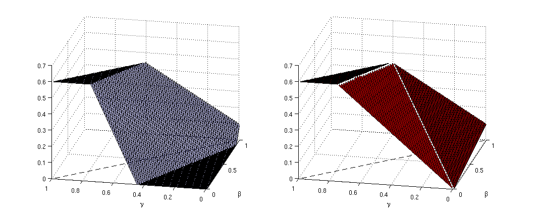
Figure 1. The modified cost function $\bar{f}(\beta,\gamma)$ on the left plotted together with the projected value function $V_{\alpha}(\beta,\gamma)$ on the right for $K_{1}=\nobreak-0.1$ and $K_{2}=0.5$. The three triangular planar regions correspond to the three cases above. It is evident that $V_{\alpha}(\beta,\gamma)$ is the concave envelope of $\bar{f}(\beta,\gamma)$.

The candidate value function $V_{\alpha}(\beta,\gamma)$ is given by

$$V_{\alpha}(\beta,\gamma)=\begin{cases}K_{2}-K_{1}&\textnormal{(i)}\quad s^{-101}\geq K_{2}\\ \frac{2\gamma+\beta}{K_{2}+1}(K_{2}-K_{1})&\textnormal{(ii)}\quad s^{01}\geq K_{2}>s^{-101}\\ \frac{\gamma}{K_{2}}(K_{2}-K_{1})&\textnormal{(iii)}\quad K_{2}>s^{01},s^{0}\leq K_{1}\\ \gamma(1-K_{1})-\beta K_{1}&\textnormal{(iv)}\quad K_{2}>s^{01},s^{0}>K_{1}\end{cases}$$

and it is the concave envelope of $\bar{f}(\beta,\gamma)$ (see Figure 1).

Appendix A Proof of Lemma 2.1

Proof.

In order to prove the independence in the $t$ variable we choose $0\leq t_{1}<t_{2}<T$ and notice that $U(t_{1},\xi)\geq U(t_{2},\xi)$. Indeed, the supremum in (2.3) corresponding to $U(t_{1},\xi)$ is taken over a larger set of stopping times than the one corresponding to $U(t_{2},\xi)$. Conversely, for any $\xi\in\Xi$ and $\tau\in\mathcal{T}_{t_{1}}$ we can choose $\tilde{\xi}\in\Xi$ and $\tilde{\tau}\in\tilde{\mathcal{T}_{t_{2}}}$ such that

$$\tilde{\tau}=a\tau+b,\qquad\tilde{\xi}_{at+b}=\xi_{t}$$

with $a=\frac{T-t_{2}}{T-t_{1}}$ and $b=\frac{T(t_{2}-t_{1})}{T-t_{1}}$. This choice leads to

$$\int x\,\xi_{\tau}(dx)=\int x\,\tilde{\xi}_{{\tilde{\tau}}}(dx)$$

which allows us to conclude that $U(t_{2},\xi)\geq U(t_{1},\xi)$ and hence $U(t_{2},\xi)=U(t_{1},\xi)$ and we have independence in $t$ for $t\in[0,T)$.

To prove the continuity in $\xi$ we first observe (e.g. see Lemma 3.1 in [6]) that if $(\xi_{r})_{r\geq 0}\in\Xi$ with $\xi_{t}=\xi$ and $d_{\mathcal{W}_{1}}(\xi_{t},\xi^{\prime})<\varepsilon$ (here $d_{\mathcal{W}_{1}}$ is the Wasserstein-1 metric) then there is $(\xi^{\prime}_{r})_{r\geq 0}\in\Xi$ with $\xi^{\prime}_{t}=\xi^{\prime}$ such that $\mathbb{E}[|\int x\,\xi_{\tau}(dx)-\int x\,\xi^{\prime}_{\tau}(dx)||\mathcal{F}_{t}]<\varepsilon$ for all $\tau\in\mathcal{T}_{t}$ with some fixed $\lambda\in\Lambda$. Indeed, we know that $\xi_{s}=\mathbb{E}[\xi_{T}|\mathcal{F}_{s}]$ and we can define

$$\xi^{\prime}_{s}(dy)=\mathbb{E}\left[\int\xi_{T}(dx)m(x,dy)|\mathcal{F}_{s}\right],\quad s\geq t,$$

where the Borel family of probability measures $m(x,dy)$ is obtained by the disintegration of the transport plan $\Gamma(dx,dy)=\xi_{t}(dx)m(x,dy)$ such that $\Gamma(\mathbb{R}_{+},dy)=\xi^{\prime}(dy)$, $\Gamma(dx,\mathbb{R}_{+})=\xi_{t}(dx)$ and $\int\int|x-y|\Gamma(dx,dy)<\varepsilon$. By optional stopping we get

$$\left|\int x\,\xi_{\tau}(dx)-\int x\,\xi^{\prime}_{\tau}(dx)\right|\leq\mathbb{E}\left[\int\int|x-y|\xi_{T}(dx)m(x,dy)|\mathcal{F}_{\tau}\right]$$

and hence

$$\mathbb{E}\left[\left|\int x\,\xi_{\tau}(dx)-\int x\,\xi^{\prime}_{\tau}(dx)\right|\Big{|}\mathcal{F}_{t}\right]\leq\int\int|x-y|\Gamma(dx,dy)<\varepsilon.$$

Denote by $M^{\xi}$ the process corresponding to the measure-valued martingale $(\xi_{r})_{r\geq 0}$ from (2.1). By the Lipschitz property of $f$ and the above inequality we get

$$\mathbb{E}\left[\left|f\big{(}M^{\xi^{\prime}}_{\tau}\big{)}-f\big{(}M^{\xi}_{\tau}\big{)}\right||\mathcal{F}_{t}\right]<\varepsilon.$$

Now fix $\varepsilon^{\prime}>0$ and consider $\xi,\xi^{\prime}\in\mathcal{P}$ such that $d_{\mathcal{W}_{1}}(\xi,\xi^{\prime})<\varepsilon^{\prime}/2$. From the reasoning above, we can choose $(\xi_{r})_{r\geq 0},(\xi^{\prime}_{r})_{r\geq 0}\in\Xi$ with $\xi_{t}=\xi$ and $\xi^{\prime}_{t}=\xi^{\prime}$ such that $U(t,\xi)\leq\sup_{\tau\in\mathcal{T}_{t}}\mathbb{E}[f\big{(}M^{\xi}_{\tau}\big{)}|\mathcal{F}_{t}]+\varepsilon^{\prime}/2$ and $\mathbb{E}\left[\left|f\big{(}M^{\xi^{\prime}}_{\tau}\big{)}-f\left(M^{\xi}_{\tau}\right)\right||\mathcal{F}_{t}\right]<\varepsilon^{\prime}/2$. Therefore we obtain

$$U(t,\xi)\leq\sup_{\tau\in\mathcal{T}_{t}}\mathbb{E}[f(M^{\xi}_{\tau})|\mathcal{F}_{t}]+\varepsilon^{\prime}/2\leq\sup_{\tau\in\mathcal{T}_{t}}\mathbb{E}[f(M^{\xi^{\prime}}_{\tau})|\mathcal{F}_{t}]+\varepsilon^{\prime}\leq U(t,\xi^{\prime})+\varepsilon^{\prime},$$

and by symmetry we get $|U(t,\xi)-U(t,\xi^{\prime})|\leq\varepsilon^{\prime}$ and continuity follows.

References

- [1] E. Bayraktar and C. W. Miller. Distribution-constrained optimal stopping. Mathematical Finance. To appear.
- [2] E. Bayraktar and M. Sirbu. Stochastic Perron’s method and verification without smoothness using viscosity comparison: the linear case. Proceedings of the American Mathematical Society, 140(10):3645–3654, 2012.
- [3] E. Bayraktar and M. Sirbu. Stochastic Perron’s method for Hamilton–Jacobi–Bellman equations. SIAM Journal on Control and Optimization, 51(6):4274–4294, 2013.
- [4] E. Bayraktar and M. Sirbu. Stochastic Perron’s method and verification without smoothness using viscosity comparison: obstacle problems and Dynkin games. Proceedings of the American Mathematical Society, 142(4):1399–1412, 2014.
- [5] M. Beiglböck, M. Eder, C. Elgert, and U. Schmock. Geometry of distribution-constrained optimal stopping problems. 2016, Preprint.
- [6] A. M. G. Cox and S. Källblad. Model-independent bounds for Asian options: a dynamic programming approach. To appear in SIAM Journal on Control and Optimization, 2017.
- [7] M. G. Crandall, H. Ishii, and P.-L. Lions. User’s guide to viscosity solutions of second order partial differential equations. Bulletin of the American Mathematical Society, 27(1):1–67, 1992.
- [8] Y. Dolinsky and H. M. Soner. Martingale optimal transport and robust hedging in continuous time. Probability Theory and Related Fields, 160(1-2):391–427, 2014.
- [9] N.V. Krylov. Controlled Diffusion Processes. Stochastic Modelling and Applied Probability. Springer Berlin Heidelberg, 2008.
- [10] A. M. Oberman. The convex envelope is the solution of a nonlinear obstacle problem. Proceedings of the American Mathematical Society, 135(6):1689–1694, 2007.
- [11] A. M. Oberman and Y. Ruan. A partial differential equation for the rank one convex envelope. Archive for Rational Mechanics and Analysis, 224(3):955–984, 2017.
- [12] G. Peskir and A. N. Shiryaev. Optimal Stopping and Free-Boundary Problems. Birkhäuser, Basel, 2006.
- [13] D. Revuz and M. Yor. Continuous Martingales and Brownian Motion. Springer, 1999.
- [14] D. B. Rokhlin. Verification by stochastic Perron’s method in stochastic exit time control problems. Journal of Mathematical Analysis and Applications, 419(1):433–446, 2014.